A Cyclical Model of Exchange Rate · PDF fileA Cyclical Model of Exchange Rate Volatility Richard D. F. Harris Evarist Stoja Fatih Yilmaz April 2010 0B0Discussion Paper No. 10/618

A Cyclical Model of Exchange Rate

Volatility

Richard D. F. Harris Evarist Stoja Fatih Yilmaz

April 2010

0B0BDiscussion Paper No. 10/618

Department of Economics University of Bristol 8 Woodland Road Bristol BS8 1TN

A Cyclical Model of Exchange Rate Volatility

Richard D. F. Harrisa, Evarist Stojab and Fatih Yilmazc

April 2010

Abstract In this paper, we investigate the long run dynamics of the intraday range of the GBP/USD, JPY/USD and CHF/USD exchange rates. We use a non-parametric filter to extract the low frequency component of the intraday range, and model the cyclical deviation of the range from the long run trend as a stationary autoregressive process. We find that the long run trend is time-varying but highly persistent, while the cyclical component is strongly mean reverting. This has important implications for modelling and forecasting volatility over both short and long horizons. As an illustration, we use the cyclical volatility model to generate out-of-sample forecasts of exchange rate volatility for horizons of up to one year under the assumption that the long run trend is fully persistent. As a benchmark, we compare the forecasts of the cyclical volatility model with those of the two-factor intraday range-based EGARCH model of Brandt and Jones (2006). Not only is the cyclical volatility model significantly easier to estimate than the EGARCH model, but it also offers a substantial improvement in out-of-sample forecast performance. Keywords: Conditional volatility; Intraday range; Hodrick-Prescott filter.

a Xfi Centre for Finance and Investment, University of Exeter, Exeter, EX4 4PU, UK. Email: [email protected] (corresponding author). b School of Economics, Finance and Management, University of Bristol, 8 Woodland Road, Bristol, BS8 1TN, UK. Email: [email protected]. c BlueGold Capital Management LLP, 2nd Floor, 4 Sloane Terrace, London SW1X 9DQ, UK. Email: [email protected].

2

1. Introduction

There is now substantial evidence that financial market volatility is both time-varying and

highly predictable (see, for example, Andersen et al., 2004). This has important

implications for many applications in finance, including portfolio optimisation, risk

measurement and option pricing, and has given rise to a large literature on volatility

measurement and forecasting. As noted by Brandt and Jones (2006), the efficacy of a

volatility model depends on a number of factors. The first is the adequacy of the proxy

for unobserved volatility that is employed in the model. Traditional volatility proxies

based on the squared demeaned return are unbiased estimators of the latent integrated

variance because the integrated volatility is, by construction, the expectation of the

squared demeaned return. However, measures based on the squared return are inefficient

owing to the fact that they employ only a single measurement of the price each period

and hence contain no information about the intra-period trajectory of the price. An

improvement in efficiency can be obtained by using intraday data. Indeed, Andersen et al.

(2004) show that under very general assumptions, the sum of squared intraday returns

converges to the unobserved integrated volatility as the intraday interval goes to zero.

However, the construction of realized volatility relies on high frequency data, which is

not readily available for most assets over extended periods. Moreover, as the intraday

frequency increases, market microstructure effects distort the measurement of returns,

leading to an upward bias in realized volatility.

An alternative volatility proxy, and one that has experienced a significant renewed

interest, is the intraday range, which is defined as the scaled difference between the

intraday high and low prices. Building on the earlier results of Parkinson (1980), Garman

and Klass (1980) and others, Alizadeh, Brandt and Diebold (2002) show that in addition

to being significantly more efficient than the squared return, the intraday range is more

robust than realized volatility to market microstructure noise. Moreover, a significant

practical advantage of the intraday range is that in contrast with the high frequency data

that are required for the construction of realized volatility, intraday high and low prices

3

are readily available for almost all financial assets over extended periods of time.1 The

intraday range has been employed in a number of conditional volatility models, including

Chou (2005), who develops a conditional autoregressive range (CARR) estimator that is

based on the conditional duration model of Engle and Russell (1998), and Brandt and

Jones (2006), who extend the EGARCH model of Nelson (1991) using the intraday range

in place of the absolute return. In both cases, the range-based GARCH estimators

generate more accurate volatility forecasts than equivalent models based on squared

returns.

The second factor that determines the efficacy of a volatility model is the specification of

the process that governs volatility dynamics. Increasingly, evidence suggests that

volatility is characterised by a multi-factor structure, with different dynamic processes

governing the long run and short run dynamics of volatility. Engle and Lee (1999)

introduce a component GARCH model, which decomposes volatility into a permanent

long-run trend component and a transitory short-run component that is mean-reverting

towards the long-run trend.2 Empirical evidence suggests that the two-factor GARCH

model provides a better fit to the data than an equivalent one-factor model. Alizadeh et al.

(2002) exploit the approximate log normality of volatility proxies based on the intraday

range and estimate both one factor and two-factor range-based stochastic volatility

models for the daily returns of a number of exchange rates using Gaussian maximum

likelihood. They find that the evidence strongly supports a two-factor model with one

highly persistent factor and one rapidly mean-reverting factor. Similarly, Brandt and

Jones (2006) estimate one-factor and two-factor range-based EGARCH models for daily

returns on the S&P 500 index. They too show that volatility is well characterised by a

two-factor model with one highly persistent factor and one strongly stationary factor.3

1 For example, Datastream records the intraday range for most securities, including equities, currencies and commodities, going back to about 1985. 2 See also Christoffersen et al (2008), who derive a two-component version of the GARCH model developed by Heston and Nandi (2000), which permits a closed-form solution for option valuation. 3 See also Gallant, Hsu and Tauchen (1999), Chernov, Ghysels, Gallant and Tauchen (2003), Barndorff-Nielsen and Shephard (2001) and Bollerslev and Zhou (2002), Maheu (2005).

4

The finding that volatility has both a highly persistent factor and a strongly stationary

factor has important implications for modelling and forecasting volatility over both short

and long horizons. In particular, using the range-based two-factor EGARCH model,

Brandt and Jones (2006) show that there is substantial predictability in volatility at

horizons of up to one year. This is in contrast with earlier studies, such as West and Cho

(1996) and Christoffersen and Diebold (1999), both of which conclude that volatility

predictability is essentially a short horizon phenomenon. It is clear that the success of

two-factor models in forecasting volatility rests on their ability to correctly identify the

current long run level of volatility, and to exploit the dynamics of the short run

component to forecast reversion of volatility to the current trend. To the extent that the

long run component is close to being non-stationary, its dynamics are only relevant, if at

all, over much longer forecasting horizons.

Motivated by the above interpretation of two-factor volatility models, we explore an

alternative, very simple approach to modelling and forecasting volatility over both short

and long horizons. In particular, we estimate the long run trend in measured volatility

using the non-parametric filter of Hodrick and Prescott (1997). We then model the

dynamics of the short run component as a stationary autoregressive process around this

long run trend. Our measure of volatility is based on the intraday range in order to exploit

the efficiency improvements that it offers over the squared return. However, rather than

apply the non-parametric filter directly to the intraday range, we separately extract the

long run components of intraday high and low prices, and then use these to construct an

estimate of the cyclical component of volatility. This is motivated by the fact that

intraday high and low prices are more likely to satisfy the assumptions of the non-

parametric filter and hence give reliable estimates of the underlying long run trend in

volatility.

We use this approach to model the volatility dynamics of the GBP/USD, JPY/USD and

CHF/USD daily exchange rates over the period 1 January 1987 to 28 April 2008.

Consistent with the findings of Engle and Lee (1999), Alizadeh et al. (2002) and Brandt

5

and Jones (2006), we show that the long run component is characterised by a time-

varying but highly persistent trend, while the short run component is strongly mean-

reverting to this trend. We use the model to generate out-of-sample forecasts of exchange

rate volatility. We assume that over the forecast horizon, the long run component of

volatility follows a random walk and use the estimated parameters of the autoregressive

model to forecast the deviation of volatility from the long run component. As a

benchmark, we compare the forecasts of our model with those of the two-factor range-

based EGARCH model of Brandt and Jones (2006), which explicitly models the long run

component of volatility parametrically as an EGARCH process. Following the approach

of Brandt and Jones (2006), we forecast volatility up to one year ahead, and use a range-

based volatility proxy to evaluate the forecasts from each model. In almost all cases, the

cyclical volatility model provides a substantial improvement in forecast performance over

the two-factor EGARCH model, in terms of both accuracy and informational content.

The improvement in performance is particularly evident over shorter horizons where the

random walk assumption for the long trend is most likely to be a good approximation. A

significant practical advantage of the cyclical volatility model is the ease with which it

can be estimated relative to other two-factor volatility models.

The outline of the remainder of this paper is as follows. In Section 2 we present the

theoretical framework. Section 3 describes the data and evaluation criteria. Section 4

presents the empirical results. Section 5 concludes.

2. Theoretical Background

Suppose that the log price of an asset,p(t), follows a continuous-time diffusion given by

dp(t) = σ 2(t)dW (t) (1)

6

where dW (t) is the increment of a Wiener process and σ 2(t) is the instantaneous

variance, which is strictly stationary and independent of dW (t) .4 Suppose that the price

is recorded at daily intervals Tt ,,1K= . Then conditional on the sample path of σ 2(t) ,

the daily logarithmic return, rt = pt − pt −1 , is normally distributed with integrated

variance σt2 = σ2(s)

t -1

t

∫ ds. The integrated variance, σt2, is unobserved, but in principle

can be estimated arbitrarily accurately using a measure of realized volatility based on

intraday returns. In particular, Andersen et al. (2004) show that under very general

conditions, the sum of squared intraday returns converges to the unobserved integrated

volatility as the intraday interval goes to zero. However, the construction of realized

volatility relies on high frequency intraday data, which are often not readily available

over extended periods. Moreover, the accuracy of realized volatility as a proxy for

integrated volatility is limited by the fact that as the intraday measurement frequency

increases, market microstructure effects distort the measurement of returns, leading to an

upward bias in estimated volatility (see, for example, Aït-Sahalia et al., 2005). An

alternative approach is to construct an estimate of volatility based on the intraday range,

given by

σR,t2 =

1

4ln2(pt

H − ptL )2 (2)

where ptH = max

t −1< s< tp(s) and pt

L = mint −1< s< t

p(s). Parkinson (1980) shows that if p(t) follows

the diffusion process given by (1), the mean square error of the range-based estimator

with respect to the true integrated variance is 5.2 times smaller than the mean square error

of the squared daily return, and is hence equivalent to using realized variance based on

intraday prices that are sampled every 4.6 hours. In practice, since prices are only

observed at discrete intervals, the sample range under-estimates the true range of the

continuous price. However, in liquid markets (such as for the major USD exchange rates

used in this paper) this bias is likely to be negligible. A significant advantage of the

4 For convenience, we assume that drift of the log price process is zero, which is a common assumption when dealing with short horizon returns. However, it is straightforward to relax this assumption.

7

estimator given by (2) is that in contrast with high frequency data, intraday high and low

prices are available on most assets over extended periods. Moreover, Alizadeh et al.

(2002) show that the range-based estimator given by (2) is relatively robust to market

microstructure noise.

In this paper, we employ the intraday range to investigate the short and long run

dynamics of daily exchange rate volatility. In particular, we assume that the square root

of the intraday range follows a two-factor process given by

σR,t = qt + α(σR ,t −1 − qt −1) +ε t (3)

where qt is the long run trend component of the intraday range, σR ,t − qt is the short run

cyclical deviation of volatility from the long run trend and ε t is a random error term with

zero mean and constant variance. The long run trend, qt , is assumed to be a stationary but

highly persistent process, but we leave its precise dynamics unspecified. The parameter

α measures the speed of reversion of the cyclical component of volatility to the long run

trend. This specification is motivated by the findings of a number of authors who show

that volatility is characterised by a factor structure (see, for example, Engle and Lee,

1999; Alizadeh et al., 2002; Brandt and Jones, 2006).

We estimate the two-factor process given by (3) in two stages. First, we estimate the

long-run component of volatility, qt , non-parametrically using the filter of Hodrick and

Prescott (1997), which extracts a low frequency non-linear trend from a time-series.

Rather than apply the filter to the intraday range itself, we estimate the long run

components of intraday high and low prices, ptH and pt

L separately. This is motivated by

the fact that intraday high and low prices are more likely to satisfy the assumptions of the

non-parametric filter and hence give reliable estimates of the underlying long run trends

in volatility. We set the smoothing parameter of the Hodrick Prescott filter to the

commonly used value of 100 multiplied by the squared frequency of the data, which for

daily data (assuming 240 trading days per year) is 5,760,000 (see, for example, Baxter

and King, 1999). This implicitly assumes that volatility is linked to the business cycle.

8

However, we also experimented with other values for the smoothing parameter and show

that our results are robust across a large range of values. Defining the long run trend

components of intraday high and low prices as ˜ p tH and ˜ p t

L , respectively, the long run

trend of volatility is constructed as

˜ q t =1

4 ln2( ˜ p t

H − ˜ p tL )2

1

2 (4)

In the second step, we estimate an autoregressive model for the cyclical component:

σR,t − ˜ q t = a(σR ,t −1 − ˜ q t −1) + v t (5)

where v t is a zero mean random error. In order to forecast volatility using the cyclical

volatility model, we assume that the long run trend follows a random walk over the

forecast horizon, so that ˜ ˆ q t + i = ˜ q t for all i > 0 , and use the estimated autoregressive

parameter from (5) to forecast the cyclical component. The n-step ahead forecast of

volatility in the cyclical volatility model is therefore given by

ˆ σ R,t +n = (1− ˆ α n ) ˜ q t + ˆ α n ˆ σ R,t (6)

As n →∞, ˆ σ R ,t +n2 → ˜ q t , with a speed that is determined by the estimated coefficient ˆ α .

The two-factor range-based EGARCH model

Brandt and Jones (2006) estimate one-factor and two-factor range-based EGARCH

models for daily returns on the S&P 500 index. They show that volatility is well

characterised by a two-factor model with one highly persistent factor and one strongly

stationary factor. As a benchmark against which to compare the cyclical volatility model,

we estimate the two-factor range-based EGARCH model, given by

9

dt ~ N(0.43+ lnσt, 0.292)

(7)

lnσt − lnσt −1 = γ1(lnqt −1 − lnσt −1) + φ1x t −1 +δ1

rt −1

σt −1

(8)

lnqt − lnqt −1 = γ2(θ − lnqt −1) + φ2x t −1 +δ2

rt −1

σ t −1

(9)

where dt = ln(ptH − pt

L ) , rt = pt − pt −1 , and x t = (dt − 0.43− lnσt ) /0.29 is the

standardised deviation of the log range from its expected value. We also estimate a one

factor range-based EGARCH model derived by setting lnqt = θ so that the long run trend

is constant. In order to forecast volatility using the EGARCH model, the shocks x t +s and

rt +s are set to zero for all s ≥1. The 1-step ahead forecast of volatility using the EGARCH

model is therefore given by

ln ˆ σ t +1 = (1− ˆ γ 1)lnσt + ˆ γ 1 lnqt + ˆ φ 1x t + ˆ δ 1rt

σt

(10)

The 2-step ahead forecast is given by

ln ˆ σ t +2 = (1− ˆ γ 1) ln ˆ σ t +1 + ˆ γ 1 ln ˆ q t +1 (11)

ln ˆ q t +1 = (1− ˆ γ 2)lnqt + ˆ γ 2 ˆ θ + ˆ φ 2x t + ˆ δ 2rt

σ t

(12)

The n-step ahead forecast for n ≥ 3 is given by

ln ˆ σ t +n = (1− ˆ γ 1) ln ˆ σ t +n −1 + ˆ γ 1 ln ˆ q t +n −1 (13)

ln ˆ q t +n = (1− ˆ γ 2)ln ˆ q t +n −1 + ˆ γ 2 ˆ θ

(14)

10

As n →∞, )ˆexp(ˆ 2 θσ →+nt , with a speed that is determined by the estimated coefficients

ˆ γ 1 and ̂ γ 2.

3. Data and Forecast Evaluation

Data

We use the cyclical volatility model to forecast volatility for the GBP/USD, JPY/USD

and CHF/USD exchange rates. Daily data were obtained for the three exchange rates

from Reuters for the period 01 January 1987 to 28 April 2008 and used to construct daily

log returns. The period 01 January 1987 to 05 December 1988 (500 observations) is

reserved for initial estimation of the volatility models, while the period 06 December

1988 to 28 April 2008 (5047 observations) is used for out-of-sample evaluation in which

the estimation window of 500 observations is rolled forward daily. Table 1 reports

summary statistics for the three log return series for the full sample of 5547 observations.

Panel A reports the mean, standard deviation, skewness and excess kurtosis coefficients

and the Bera-Jarque statistic, while Panel B reports the first six autocorrelation

coefficients and the Ljung-Box Q statistic for autocorrelation up to six lags for both

returns and squared returns. P-values are reported in parentheses. All three series are

highly non-normal with positive excess kurtosis and negative skewness. The return series

are serially uncorrelated, but squared returns are highly autocorrelated, indicative of

volatility clustering.

[Table 1]

Panel A of Figure 1 plots the intraday range measure of standard deviation over the

whole sample of 5547 observations together with the long run trend estimated using the

Hodrick-Prescott filter. Panel B of Figure 1 plots the resulting cyclical component of the

standard deviation. It is clear that the long run trend in volatility is time-varying and

highly persistent, while the cyclical component is strongly mean-reverting, lending

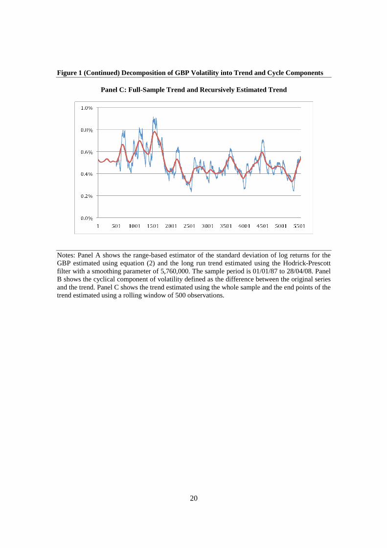
support to the two-component representation of volatility. Panel C of Figure 1 plots the

11

recursively estimated endpoint of the trend, which is used for forecasting volatility out-

of-sample, together with the trend estimated using the full sample. The recursively

estimated trend is more volatile than the full-sample trend owing to the fact that at the

end point of each rolling sample, the Hodrick-Prescott filter is implemented as a one-

sided filter, while for the corresponding observation within the full sample, it is a

implemented as a two-sided filter which exploits information contained in subsequent

observations to identify the trend ex post.

[Figure 1]

Forecast evaluation

Each of the two models is used to generate out-of-sample forecasts of the standard

deviation of returns for horizons of up to 240 days over the evaluation period. The

models are initially estimated using the first five hundred observations, and then the

estimation period is rolled forward daily until the end of the sample is reached. Following

Brandt and Jones (2006), from the point forecasts made at date t, we construct average

forecasts of the standard deviation between t +τ1 and t +τ2:

ˆ σ t (τ1,τ 2) =1

τ2 −τ1 +1ˆ σ t +τ

τ =τ1

τ2

∑ (15)

We consider forecast horizons of 1, 5, 20, 60, 120 and 240 days. For the three shorter

horizons, we take the average over the forecast horizon, i.e. (τ1,τ2) = (1, 1), (1, 5) and (1,

20). For the three longer horizons, we use monthly averages, i.e. (τ1,τ2) = (41,60), (101,

120) and (221, 240). As a proxy for true volatility, we use the square root of the range-

based estimator of the variance given by (2). This is used to construct the average

volatility over the each of the six forecast intervals:

σt (τ1,τ 2) =1

τ2 −τ1 +1σR ,t +τ

τ =τ1

τ2

∑ (16)

12

We evaluate the forecasting performance of the non-overlapping conditional variance

forecasts ̂ σ i,t (τ1,τ2) generated by model i using two measures. The first is the root mean

square error (RMSE) with respect to the true average volatility:

RMSE =1T

(σt (τ1,τ2) − ˆ σ i,t (τ1,τ2))2

t =1

T

∑

1/ 2

(17)

The second criterion is the Mincer and Zarnowitz (1969) regression for each model given

by:

σt (τ1,τ 2) = α i + βiˆ σ i,t (τ1,τ2) +ε i,t (τ1,τ2) (18)

The Mincer-Zarnowitz regression measures the efficiency of the forecasts from each

model. In particular, if the model is weakly efficient, α i = 0 and βi =1. We test the null

hypothesis of weak efficiency for each model i and for each forecast interval, (τ1,τ2). The

R-squared coefficient from the Mincer-Zarnowitz regression reveals the explanatory

power of the model, irrespective of its efficiency, and is thus a useful measure of the

information content of a model’s forecasts.

4. Results

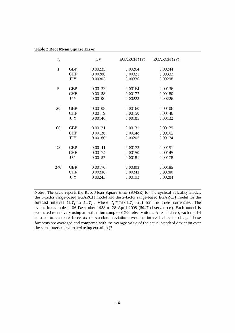
Table 2 reports the RMSE given by (17) for the three conditional volatility models over

the different forecasting intervals for the three currencies. Across all three models, the

RMSE at first falls with the forecast horizon and then rises. This is explained by the fact

that initially, the forecast interval increases from 1 day to 5 days and then to 20 days. By

averaging forecasts over increasingly long intervals, the noise in the forecasts is reduced,

and this tends to outweigh any reduction in accuracy arising from an increase in the

forecast horizon. After the 20-day horizon, the forecast interval is fixed at 20 days, and so

forecast accuracy reduces as the horizon increases. For the 2-factor EGARCH model, the

deterioration in forecast accuracy is very pronounced at the 240-day horizon. Overall, the

13

cyclical model offers the highest forecast accuracy in 12 of the 18 cases, followed by the

2-factor EGARCH model in five of the 18 cases. In only one case does the 1-factor

EGARCH offer the lowest RMSE, which is consistent with the component representation

of volatility.

[Table 2]

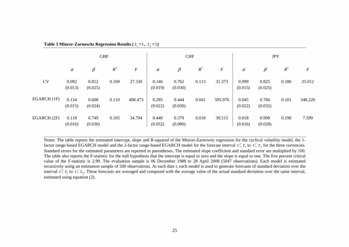
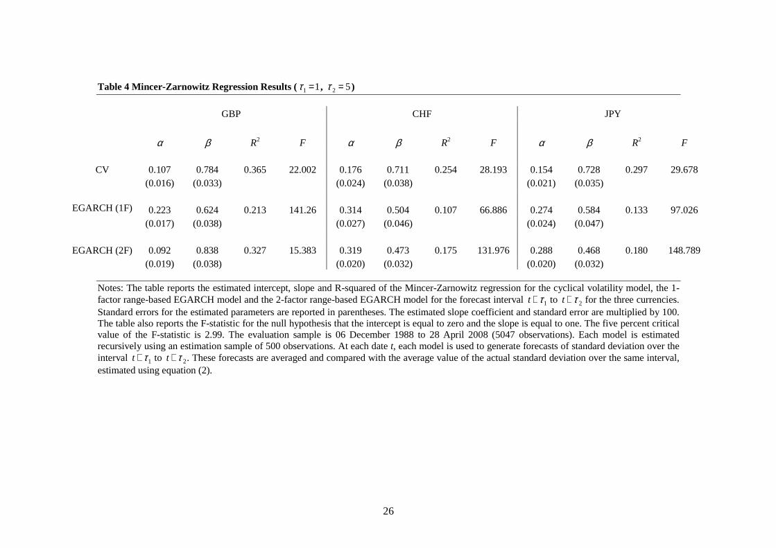
Tables 3 to 8 report the estimation results of the Mincer-Zarnowitz regression given by

(18). The tables report the estimated regression parameters, the standard errors of these

estimates, the regression R-squared statistic and the F-statistic to test the null hypothesis

of conditional unbiasedness. In line with the results for the RMSE reported in Table 2,

the R-squared generally increases for horizons up to 20 days, and then falls, reflecting

initially the reduction in noise from extending the interval over which the forecasts are

averaged, and then a reduction in performance from extending the forecasting horizon.

For the short horizon forecasts (Tables 3 to 5), the cyclical volatility model has

substantial explanatory power. Across all three currencies, the average value of the R-

squared statistic is 15.4% for the one-day forecasts, 30.5% for the five-day forecasts and

38.3% for the 20-day forecasts. The explanatory power for the two-factor EGARCH

model is generally considerably lower (10.7%, 22.7% and 31.8%, respectively), and for

the one-factor EGARCH model, lower still (8.4%, 15.1% and 18.9%, respectively). Of

the nine short horizon forecasts, the highest explanatory power is offered by the cyclical

volatility model in seven cases, and by the two-factor EGARCH model in two cases.

However, where the explanatory power of the two-factor EGARCH model is higher than

that of the cyclical volatility model, the differences are relatively small. The highest

explanatory power for short horizon forecasts of any of the three models is 43.5% for the

20-day forecasts of the cyclical volatility model for the GBP. In all cases, the estimated

slope coefficient is lower than unity and declines monotonically with the forecast horizon.

The null hypothesis of conditional unbiasedness is rejected in all cases at the five percent

significance level, but the rejection is notably stronger for the one-factor EGARCH

model than for either of the two-factor models.

14

[Tables 3 to 5]

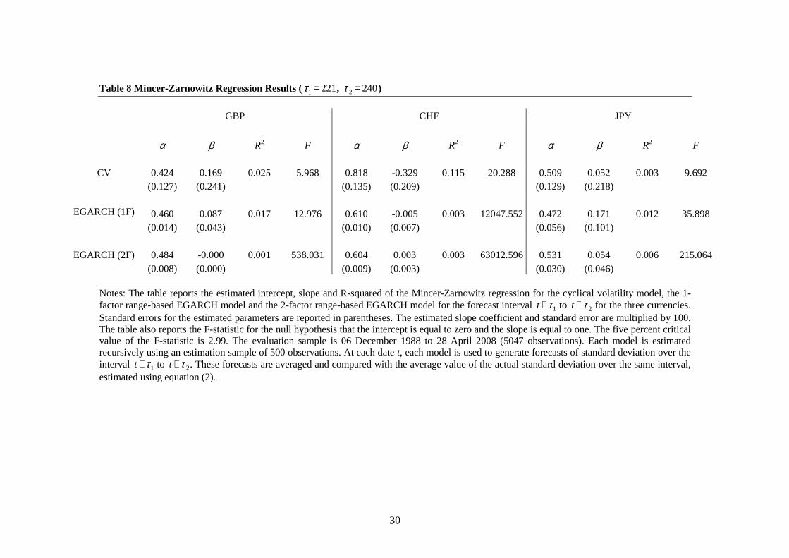
For the long horizon forecasts (Tables 6 to 8), the explanatory power of the three models

declines relative to the 20-day forecasts as the forecast horizon increases. For the cyclical

model, the average R-squared statistic across the three currencies is 22.2% for 60-day

forecasts, 10.1% for 120-day forecasts and 4.8% for 240-day forecasts. Again, this is

higher than either of the two EGARCH models. In many cases, the two-factor EGARCH

model has higher explanatory power than the one-factor EGARCH model, although the

differences are generally small. At the 240-day horizon, the explanatory power of the

two-factor EGARCH model falls to zero for all three currencies. In contrast, the cyclical

volatility model is able to explain 11.5% of the variation in volatility for the CHF at the

240-day horizon. Note, however, that the estimated slope coefficients fall significantly

over longer forecast horizons, and indeed for the CHF at the 240-day horizon, the

estimated slope coefficient is significantly negative for the cyclical volatility model.

[Tables 6 to 8]

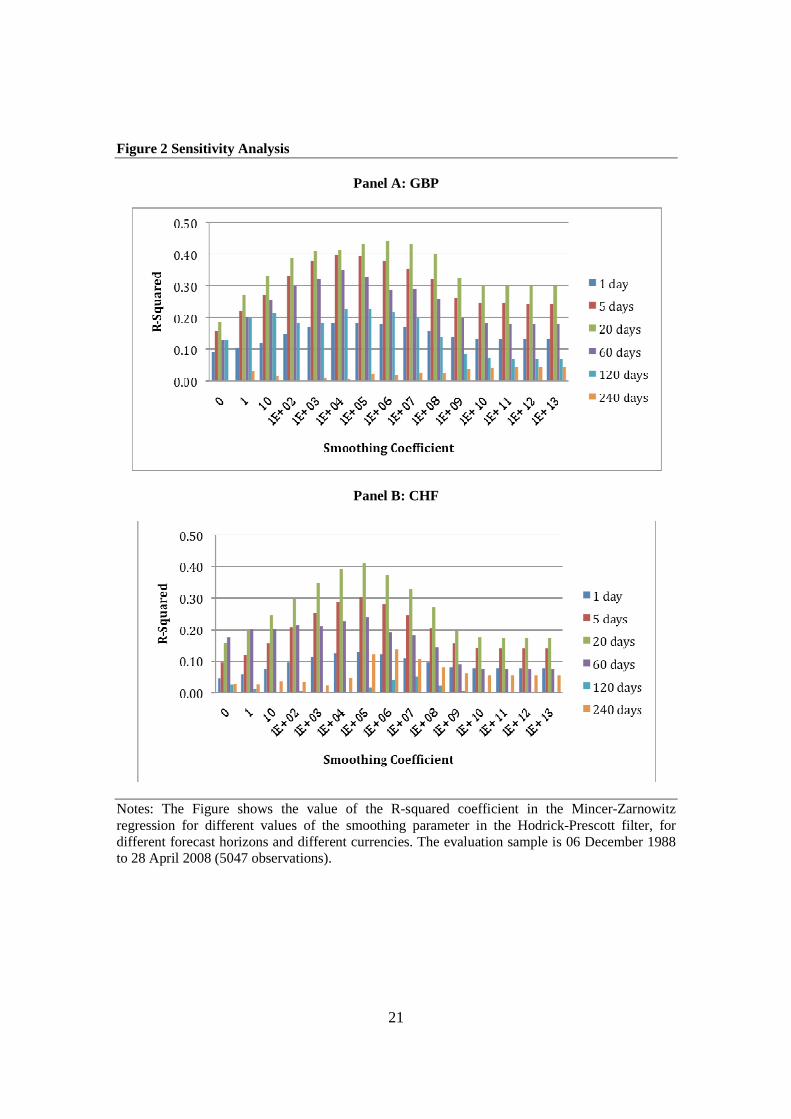
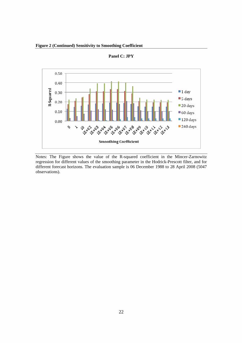
We now explore the sensitivity of the cyclical model’s performance to the choice of

smoothing parameter in the Hodrick-Prescott filter. In particular, Figure 2 reports the R-

squared coefficient from the Mincer-Zarnowitz regression for values of the smoothing

parameter from zero to 1013. Results are reported for each currency and for each of the

six different forecast intervals. A smoothing parameter of zero corresponds to no trend. In

this case, the forecast of the next period’s volatility is simply equal to the current period’s

volatility. As the smoothing parameter increases, the estimated trend becomes more

linear. With a smoothing parameter of 1013 – the highest value that we consider – the

trend estimated over the full sample is visually indistinguishable from a linear trend.

Figure 2 reveals that forecast performance at first increases with the value of the

smoothing parameter and then decreases, and that this is true for all six forecast horizons

and for all three currencies. In almost all cases, the optimal smoothing parameter is

between 104 and 106. This is reasonably close to the smoothing parameter used in the

results reported above (0.576x107) and for the GBP and JPY, the reduction in

15

performance from using the higher value is relatively small. For the CHF, the difference

is more pronounced. Although not reported, a similar pattern emerges for the RMSE of

the model’s forecasts, with the most accurate forecasts generated by intermediate value of

the smoothing parameter. Indeed, the optimal value of the smoothing parameter in terms

of RMSE appears to be even closer to the ‘default’ value that we have used.

[Figure 2]

5. Conclusion

The finding that volatility has both a highly persistent component and a strongly

stationary component has important implications for modelling and forecasting volatility

over both short and long horizons. In this paper, we develop a simple yet effective model

for forecasting volatility that is based on a decomposition of the intraday range measure

of volatility into its trend and cycle components. Using a non-parametric filter, we are

able to estimate the long run trend in volatility without having to specify its dynamics.

Modelling the cyclical deviation of volatility from the long run trend as a simple

autoregressive process then allows us to forecast volatility under the assumption that the

trend component follows a random walk over the forecast horizon. We show that out-of-

sample forecasts generated by the cyclical volatility model are able to explain a

substantial fraction of the variation in actual volatility at horizons of up to one year. The

model generally outperforms the two-factor range-based EGARCH model of Brandt and

Jones (2006), in terms of both forecast accuracy and informational content. Owing to its

simplicity, the cyclical volatility model also offers a substantial computational advantage

over the two-factor EGARCH model. Indeed, the estimation time for the cyclical

volatility model was many orders of magnitude lower than for the EGARCH model.

The results reported in this paper, as encouraging as they are, are based on the simplest

possible specification both for the long run trend component (which we leave unspecified

but assume to follow a random walk over the forecast horizon) and the cyclical

component (which we assume to follow a first order autoregressive process). A natural

16

line of further investigation would be alternative specifications for these two components.

Almost certainly, a higher order ARMA process would provide a better fit for the cyclical

component in-sample, and consequently it would be interesting to establish whether this

translates into an improvement in out-of-sample forecast performance. Similarly, in order

to estimate the long run trend, we have employed the ‘default’ value of the smoothing

parameter in the Hodrick-Prescott filter, thus linking the trend in volatility to the trend in

the business cycle. While this is perhaps a reasonable assumption, it is clear from the

results reported above that this is not the optimal value, and so it would be interesting to

estimate this parameter from the data. Moreover, while the random walk assumption for

the long run trend provides a good approximation for short horizon forecasts, it becomes

increasingly unrealistic as the forecast horizon increases since the long run trend, while

highly persistent is nevertheless stationary and hence mean-reverting. It would be

straightforward to adapt the specification of the cyclical model to incorporate these

dynamics. A further avenue for future research would be to extend the cyclical volatility

model to the multivariate setting.

17

References Aït-Sahalia, Y., P. Mykland, and L. Zhang, 2005, “How Often to Sample a Continuous-Time Process in the Presence of Market Microstructure Noise”, Review of Financial Studies 18, 351-416. Alizadeh, S., M. Brandt and F. Diebold, 2002, “Range-Based Estimation of Stochastic Volatility Models”, Journal of Finance 57, 1047–92. Andersen, T., T. Bollerslev and F. Diebold, 2004, “Parametric and Nonparametric Measurements of Volatility”, In: Aït-Sahalia, Y., Hansen, L.P. (Eds.), Handbook of Financial Econometrics, North-Holland, Amsterdam. Baxter, M., and R. King, 1999, “Measuring Business Cycles: Approximate Band-Pass Filters for Economic Time Series”, Review of Economics and Statistics 81, 575-593. Barndorff-Nielsen, O., and N. Shephard, 2001, “Non-Gaussian Ornstein-Uhlenbeck–Based Models and Some of Their Uses in Financial Economics”, Journal of the Royal Statistical Society Series B 63, 167–241. Bollerslev, T., and H. Zhou, 2002, “Estimating Stochastic Volatility Diffusions Using Conditional Moments of Integrated Volatility”, Journal of Econometrics 109, 33–65. Brandt, M., and F. Diebold, 2006, “A No-Arbitrage Approach to Range-Based Estimation of Return Covariances and Correlations”, Journal of Business 79, 61–74. Chernov, M., E. Ghysels, A. Gallant, and G. Tauchen, 2003, “Alternative Models for Stock Price Dynamics”, Journal of Econometrics 106, 225–257. Chou, R., 2005, “Forecasting Financial Volatilities with Extreme Values: The Conditional Autoregressive Range (CARR) Model”, Journal of Money, Credit and Banking 37, 561-582. Christoffersen, P., and F. Diebold, 2000, “How Relevant Is Volatility Forecasting for Financial Risk Management?” Review of Economics and Statistics 82, 1–11. Christoffersen, P., K. Jacobs, C. Ornthanalai and Y. Wang, 2008, “Option Valuation with Long-run and Short-run Volatility Components”, Journal of Financial Economics 90, 272-297. Engle, R., and G. Lee, 1999, “A Permanent and Transitory Model of Stock Return Volatility”, in Cointegration, Causality, and Forecasting: A Festschrift in Honor of Clive W. J. Granger, eds. R. F. Engle and H. White, New York: Oxford University Press, pp. 475–497.

18

Engle, R., and J. Russell, 1998, “Autoregressive Conditional Duration: A New Model for Irregular Spaced Transaction Data”, Econometrica 66, 1127-1162. Gallant, A, C. Hsu, and G. Tauchen, 1999, “Using Daily Range Data to Calibrate Volatility Diffusions and Extract the Forward Integrated Variance”, Review of Economics and Statistics 81, 617–631. Garman, M., and M. Klass, 1980, “On the Estimation of Price Volatility from Historical Data”, Journal of Business 53, 67–78. Heston, S., and S. Nandi, 2000, “A Closed-Form GARCH Option Pricing Model”, Review of Financial Studies 13, 585-626. Hodrick, R., and E. Prescott, 1997, Post-War US Business Cycles: An Empirical Investigation”, Journal of Money, Credit and Banking 29, 1-16. Maheu, J., 2005, “Can GARCH Models Capture Long-Range Dependence?” Studies in Nonlinear Dynamics and Econometrics 9, Article 1. Nelson, D., 1991, “Conditional Heteroskedasticity in Asset Returns: A New Approach”, Econometrica 59, 347-370. Parkinson, M., 1980, “The Extreme Value Method for Estimating the Variance of the Rate of Return”, Journal of Business 53, 61–65. West, K., and D. Cho, 1995, “The Predictive Ability of Several Models of Exchange Rate Volatility”, Journal of Econometrics 69, 367–391.

19

Figure 1 Decomposition of GBP Volatility into Trend and Cycle Components

Panel A: Volatility and Long Run Trend

Panel B: Cyclical Component of Volatility

Notes: Panel A shows the range-based estimator of the standard deviation of log returns for the GBP estimated using equation (2) and the long run trend estimated using the Hodrick-Prescott filter with a smoothing parameter of 5,760,000. The sample period is 01/01/87 to 28/04/08. Panel B shows the cyclical component of volatility defined as the difference between the original series and the trend. Panel C shows the trend estimated using the whole sample and the end points of the trend estimated using a rolling window of 500 observations.

20

Figure 1 (Continued) Decomposition of GBP Volatility into Trend and Cycle Components

Panel C: Full-Sample Trend and Recursively Estimated Trend

Notes: Panel A shows the range-based estimator of the standard deviation of log returns for the GBP estimated using equation (2) and the long run trend estimated using the Hodrick-Prescott filter with a smoothing parameter of 5,760,000. The sample period is 01/01/87 to 28/04/08. Panel B shows the cyclical component of volatility defined as the difference between the original series and the trend. Panel C shows the trend estimated using the whole sample and the end points of the trend estimated using a rolling window of 500 observations.

21

Figure 2 Sensitivity Analysis

Panel A: GBP

Panel B: CHF

Notes: The Figure shows the value of the R-squared coefficient in the Mincer-Zarnowitz regression for different values of the smoothing parameter in the Hodrick-Prescott filter, for different forecast horizons and different currencies. The evaluation sample is 06 December 1988 to 28 April 2008 (5047 observations).

22

Figure 2 (Continued) Sensitivity to Smoothing Coefficient

Panel C: JPY

Notes: The Figure shows the value of the R-squared coefficient in the Mincer-Zarnowitz regression for different values of the smoothing parameter in the Hodrick-Prescott filter, and for different forecast horizons. The evaluation sample is 06 December 1988 to 28 April 2008 (5047 observations).

23

Table 1 Summary Statistics and Autocorrelations

Panel A: Summary Statistics

Mean

Standard Deviation

Skewness

Excess Kurtosis

Bera-Jarque

GBP 0.005% 0.589% -0.207 3.050 662.268 CHF -0.008% 0.715% -0.112 1.701 763.295 JPY -0.007% 0.689% -0.494 5.213 839.624

Panel B: Autocorrelations

Returns 1 2 3 4 5 6

Q

GBP -0.010 0.031 -0.014 -0.039 0.065 0.024 0.694 (0.994) CHF -0.001 -0.128 0.043 -0.042 0.003 -0.000 1.745 (0.941) JPY 0.059 -0.095 -0.074 -0.072 0.032 0.007 2.122 (0.908)

Squared Returns

1 2 3 4 5 6

Q

GBP 0.094 0.131 0.093 0.092 0.097 0.108 354.792 (0.000) CHF 0.086 0.028 0.042 0.054 0.052 0.097 136.496 (0.000) JPY 0.142 0.078 0.043 0.071 0.059 0.071 229.822 (0.000)

Notes: Panel A reports the mean, standard deviation, skewness, excess kurtosis and the Bera-Jarque statistic for daily log close-to-close returns for GBP/USD, CHF/USD and JPY/USD. The sample period is 01/01/87 to 28/04/08. Panel B reports the first six autocorrelation coefficients and the Ljung-Box Q statistic for autocorrelation up to six lags, for both returns and squared returns. P-values are reported in parentheses.

24

Table 2 Root Mean Square Error

τ 2 CV EGARCH (1F) EGARCH (2F) 1 GBP 0.00235 0.00264 0.00244 CHF 0.00280 0.00321 0.00333 JPY 0.00303 0.00336 0.00298 5 GBP 0.00133 0.00164 0.00136 CHF 0.00158 0.00177 0.00180 JPY 0.00190 0.00223 0.00226

20 GBP 0.00108 0.00160 0.00106 CHF 0.00119 0.00150 0.00146 JPY 0.00146 0.00185 0.00132

60 GBP 0.00121 0.00131 0.00129 CHF 0.00136 0.00148 0.00161 JPY 0.00160 0.00205 0.00174

120 GBP 0.00141 0.00172 0.00151 CHF 0.00174 0.00150 0.00145 JPY 0.00187 0.00181 0.00178

240 GBP 0.00170 0.00303 0.00185 CHF 0.00236 0.00242 0.00280 JPY 0.00243 0.00193 0.00284

Notes: The table reports the Root Mean Square Error (RMSE) for the cyclical volatility model, the 1-factor range-based EGARCH model and the 2-factor range-based EGARCH model for the forecast interval t + τ1 to t +τ 2 , where τ1 = max(1,τ 2 − 20) for the three currencies. The evaluation sample is 06 December 1988 to 28 April 2008 (5047 observations). Each model is estimated recursively using an estimation sample of 500 observations. At each date t, each model is used to generate forecasts of standard deviation over the interval t + τ1 to t + τ 2 . These forecasts are averaged and compared with the average value of the actual standard deviation over the same interval, estimated using equation (2).

25

Table 3 Mincer-Zarnowitz Regression Results ( τ1 =1, τ 2 =1) GBP CHF JPY

α β R2 F α β R2 F α β R2 F

CV 0.092 0.812 0.169 27.330 0.146 0.762 0.113 31.373 0.099 0.825 0.180 25.012 (0.013) (0.025) (0.019) (0.030) (0.015) (0.025)

EGARCH (1F) 0.134 0.608 0.110 498.473 0.285 0.444 0.041 595.976 0.045 0.766 0.101 348.220 (0.015) (0.024) (0.022) (0.030) (0.022) (0.032)

EGARCH (2F) 0.118 0.749 0.105 34.794 0.440 0.379 0.018 39.515 0.018 0.998 0.198 7.599 (0.016) (0.030) (0.052) (0.080) (0.016) (0.028)

Notes: The table reports the estimated intercept, slope and R-squared of the Mincer-Zarnowitz regression for the cyclical volatility model, the 1-factor range-based EGARCH model and the 2-factor range-based EGARCH model for the forecast interval t +τ1 to t + τ 2 for the three currencies. Standard errors for the estimated parameters are reported in parentheses. The estimated slope coefficient and standard error are multiplied by 100. The table also reports the F-statistic for the null hypothesis that the intercept is equal to zero and the slope is equal to one. The five percent critical value of the F-statistic is 2.99. The evaluation sample is 06 December 1988 to 28 April 2008 (5047 observations). Each model is estimated recursively using an estimation sample of 500 observations. At each date t, each model is used to generate forecasts of standard deviation over the interval t + τ1 to t +τ 2. These forecasts are averaged and compared with the average value of the actual standard deviation over the same interval, estimated using equation (2).

26

Table 4 Mincer-Zarnowitz Regression Results ( τ1 =1, τ 2 = 5) GBP CHF JPY


CV 0.107 0.784 0.365 22.002 0.176 0.711 0.254 28.193 0.154 0.728 0.297 29.678 (0.016) (0.033) (0.024) (0.038) (0.021) (0.035)

EGARCH (1F) 0.223 0.624 0.213 141.26 0.314 0.504 0.107 66.886 0.274 0.584 0.133 97.026 (0.017) (0.038) (0.027) (0.046) (0.024) (0.047)

EGARCH (2F) 0.092 0.838 0.327 15.383 0.319 0.473 0.175 131.976 0.288 0.468 0.180 148.789 (0.019) (0.038) (0.020) (0.032) (0.020) (0.032)


27

Table 5 Mincer-Zarnowitz Regression Results ( τ1 =1, τ 2 = 20) GBP CHF JPY


CV 0.147 0.703 0.435 17.195 0.230 0.623 0.338 23.325 0.202 0.641 0.375 23.489 (0.026) (0.051) (0.034) (0.055) (0.031) (0.052)

EGARCH (1F) 0.274 0.550 0.243 116.972 0.393 0.351 0.107 51.523 0.317 0.504 0.218 66.265 (0.025) (0.061) (0.040) (0.064) (0.031) (0.060)

EGARCH (2F) 0.115 0.784 0.398 8.063 0.371 0.406 0.147 50.588 0.090 0.864 0.408 3.937 (0.030) (0.061) (0.037) (0.062) (0.037) (0.066)


28

Table 6 Mincer-Zarnowitz Regression Results ( τ1 = 41, τ 2 = 60) GBP CHF JPY


CV 0.231 0.519 0.290 14.434 0.339 0.442 0.183 14.630 0.332 0.378 0.193 27.050 (0.045) (0.090) (0.064) (0.103) (0.049) (0.085)

EGARCH (1F) 0.240 0.514 0.261 39.412 0.405 0.336 0.076 39.997 0.420 0.249 0.057 68.766 (0.028) (0.055) (0.046) (0.074) (0.039) (0.064)

EGARCH (2F) 0.217 0.539 0.257 34.069 0.427 0.292 0.091 74.120 0.298 0.467 0.170 33.355 (0.030) (0.058) (0.037) (0.058) (0.039) (0.066)


29

Table 7 Mincer-Zarnowitz Regression Results ( τ1 =101, τ 2 =120) GBP CHF JPY

a b R2 F a b R2 F a b R2 F

CV 0.257 0.483 0.208 6.000 0.458 0.241 0.052 10.949 0.428 0.182 0.042 17.976 (0.076) (0.149) (0.101) (0.162) (0.078) (0.138)

EGARCH (1F) 0.346 0.317 0.159 119.087 0.336 0.407 0.038 35.985 0.390 0.302 0.030 21.259 (0.022) (0.046) (0.088) (0.131) (0.064) (0.109)

EGARCH (2F) 0.307 0.386 0.169 66.070 0.347 0.405 0.068 29.827 0.353 0.365 0.047 19.499 (0.027) (0.055) (0.063) (0.096) (0.062) (0.105)


30

Table 8 Mincer-Zarnowitz Regression Results ( τ1 = 221, τ 2 = 240) GBP CHF JPY


CV 0.424 0.169 0.025 5.968 0.818 -0.329 0.115 20.288 0.509 0.052 0.003 9.692 (0.127) (0.241) (0.135) (0.209) (0.129) (0.218)

EGARCH (1F) 0.460 0.087 0.017 12.976 0.610 -0.005 0.003 12047.552 0.472 0.171 0.012 35.898 (0.014) (0.043) (0.010) (0.007) (0.056) (0.101)

EGARCH (2F) 0.484 -0.000 0.001 538.031 0.604 0.003 0.003 63012.596 0.531 0.054 0.006 215.064 (0.008) (0.000) (0.009) (0.003) (0.030) (0.046)


Documents

A Cyclical Model of Exchange Rate · PDF fileA Cyclical Model of Exchange Rate Volatility Richard D. F. Harris Evarist Stoja Fatih Yilmaz April 2010 0B0Discussion Paper No. 10/618