FD-A184 972 DEVELOPMENTVOF A DATA ANALYSIS SYSTEM FOR THE DETECTION 1/2OF LOWER LEVEL AT (U) NAVAL POSTGRADUATE SCHOOL

CLSIID MONTEREY CA M R WROBLEWJSKI JUN 87

UNCSSFE 7 /G 4/1 NENENEmoEsooEEEEEEEEEEEEEEEEohhohhhhmhhhIEhhhhmmEmhEshIsommIEEEEEWIEE.EEEEEE.EEEcohE

L

1111I .25 111.4 16lii. 111-11U11

MICROCOPY RESOLUTION TEST CHARTNATIONAL BUREAL, OF SIANDAR[DS 1963 A

N

NAVAL POSTGRADUATE SCHOOLMonterey, California OTC FILE COPY

DT[CS'ELECTEO

%:D

THESIS&

DEVELOPMENT OF A DATA ANALYSIS SYSTEMFOR THE DETECTION OF

LOWER LEVEL ATMOSPHERIC TURBULENCEWITH AN ACOUSTIC SOUNDER

by

Michael Raymond Wroblewski

June 1987

Thesis Advisor: D. L. Walters

Approved for public release; distribution is unlimited

- 13

S(CLRI1'Y CLASSIFICATION 09 TmTI PAGE

REPORT DOCUMENTATION PAGE'a REPORT SECuRITY CLASSIFICATION lb RESTICTIVE MARICINGS

Unclassified ___________________

2a SECURITY CLASSIFICATION AUTHORITY I DISTRIBUTION'/AVAILABILITY OF REPORT

2b ECLSS,,CA;ON DWNGADIG SHEDLEApproved for public release;2b DCLASIFCATON OWNRADNG CHEULEdistribution is unlimited

4 PERFORMING ORGANIZATION REPORT NUMBER(S) S MONITORING ORGANIZATION REPORT NUMBER(S)

6a NAME OF PERFORMING ORGANIZATION 160 OFFICE SYMBOL 7a NAME OF MONITORING ORGANIZATION(it apicable)

Naval Postgraduate School 61 Naval Postgraduate School6( ADDRESS C,1y Star* and ZIP Code) 7b ADDRESS (City, State. anid ZIP Code)

Monterey, California 93943-5000 Monterey, California 93943-5000

Sa NAME OF FUNDiNG,SPONSORiNG ID OFFICE SYMBOL 9 PROCUREMENT INSTRuMENT IDENTIFICATION NIUMBERORGANIZATION j (if applicable)

Sc ADDRESS(Cry State, anid ZIP Code) 10 SOURCE 0; FUNDING NUMBERS

PROGRAM PROIECT ITASK( WORK jNiTELEMENT NO INO NO ACCESS;ON NO

T 'E (include Secuisry Claifcarbon)

DEVELOPMENT OF A DATA ANALYSIS SYSTEM FOR THE DETECTION OFLOWER LEVEL ATMOSPHERIC TURBULENCE WITH AN ACOUSTIC SOUNDER

* PERSONA, AUTt4OR(S)

Wroblewski, Michael R..3 'vP 0; REPORT '30 ME V~ERED 14 DATE OF REPORT (Year M~onth Day) 5 PAGE (OI-NT

Maste I s TOsi 197 Jn 106 Sk-PPEVENTARY NOTAT:ON

*'COSAT, CODES lB SuBjECT TERP.S (Continue on reverle of nececsary and ieiIf by block "umbor)

I ELD GROUP SuB-GROuP Acoustic Radar, Echosounder, AcousticSounder, Atmospheric Turbulence Profiles

1 .SrRAC (COntinue on fillviti if neCCuary and identify byr block number)

Atmospheric density fluctuations induce phase perturbationsthat degrade the spatial coherence of a laser beam propagatingthrough the atmoshpere. These degradations spread the laserbeam and alter the centroid and intensity profile stochastically.Turbulent conditions are found at virtually all levels of theatmosphere. A substantial fraction of the optical turbulencealong a vertical path arises from the heat flux between theatmosphere and the Earth's surface. This type of turbulence istypically within the first 100 to 200 meters above the surface.

During this thesis research, a high frequency acousticsounder was developed to analyze this turbulent layer. The

3 D P 3,j ON, AVAILABILITY OF ABSTRACT 121 ABTATSECURITY CL.ASSIFICATION

Xj -NCASSIF EDUINL MITED 0 SAME AS RPT QOTC SFR S I Unclassified _____________

,') %AME 0' RESPONSIBLE %D~\iIDuAL 22b TELEPNONE(lInclude Area Code 22c OFF (k SM80',

Donald L. Walters 408-646-2267 1 6lWe00 FORM 1473. 84 MAR 83 APR ed~ton -ay be uted vi'l 0whausted SECURITY CLASS1FsCAr1ON OF 'HIS PACE

All other edt-OM a(* obtoltt

SCCURiTY CLASSIFICATION OF THIS PAd9 (ft,0m0m DM bmeee

19. (continued)

primary focus was the development of the command and controlsoftware required to coordinate the data collection andreduction. The system was used at two sites and shouldprove useful in quantifying the effects of optical turbulencewithin the surface boundary layer on laser and opticalsystem performance.

IECUtITY CLASSIFICATION OF THIS5 PAGU(Wbef 0010 Entered)

Approved for public release: distribution is unlimited.

Development of a Data Analysis System for theDetection of Lower Level Atmospheric Turbulence

with an Acoustic Sounder

by

Michael Raymond WroblewskiLieutenant, United States Coast Guard

B.S. , United States Coast Guard Academy, 1980

Submitted in partial fulfillment of therequirements for the degree of

MASTER OF SCIENCE IN PHYSICS

from the

NAVAL POSTGRADUATE SCHOOLJune 1987

Author: __ _ _ _ _ __ _ _ _ _ _ __ _ __1_ __ _ _ _ _ _

Michael R. Wroblewski

Approved by: 4V k W iho s

Donald L. Walters, Thesis Advisor

Edmund A Milne, S-cond Reader

Karlhein- . oehler, Chairman,Depart ent of Physics

Gordon E. Schacher, Dean of Science andEngineering

3

ABSTRACT

_z Atmospheric density fluctuations induce phase

perturbations that degrade the spatial coherence of a laser

beam propagating through the atmosphere. These

degradations spread the laser beam and alter the centroid

and intensity profile stochastically. Turbulent conditions

are found at virtually all levels of the atmosphere. A

substantial fraction of the optical turbulence along a

vertical path arises from the heat flux between the

atmosphere and the Earth's surface. This type of

turbulence is typically within the first 100 to 200 meters

above the surface.

During this thesis research, a high frequency acoustic

sounder was developed to analyze this turbulent layer. The

primary focus was the development of the command and

control software required to coordinate the data collection

and reduction. The system was used at two sites and should

prove useful in quantifying the effects of optical

turbulence within the surface boundary layer on laser and

optical system performance.

4

TABLE OF CONTENITS

I. INTRODUCTION........................................ 7

II. BACKGROUND......................................... 1

111. SYSTEM DESIGN AND EQUIPMENT DEVELOPMENT ...... 14

A. HARDWARE........................................ 14

B. SOFTWARE....................................... 19

IV. DATA ANALYSIS...................................... 25

A. ECHOSjOrNDER PERFORMANCE........................ 25

B. SITE EVALUATION................................ 25

V. CONCLUSIONS AND RECOMMENDATIONS.................... 40

APPENDIX A ACOUSTIC ECHOSOUNDER PROGRAM................. 42

APPENDIX B SPEAKER AND ARRAY ANALYSIS................... 60

APPENDIX C ENCLOSURE DESIGN............................. .70

APPENDIX D ECHOSOUNDER OUTPUT........................... .79

LIST OF REFERENCES....................................... 9

INITIAL DISTRIBUTION LIST ............... 1

Accesion For

NTIS CRA&J000DTIC T/r3 Q

B y J i .. .............

%urrj~.

ACKNOWLEDGEMENTS

I express my gratitude to all who have made my

graduation from the Naval Postgraduate School a reality.

First and foremost I would like to thank my wife, Beth.

Without her support and love I doubt I ever would have been

able to accomplish this task.

I would also like to say "Thanks' to Professor Donald

Walters who gave of his time and knowledge. He supplied us

with the tools and motivation (As he always said: "Well, if

you want to graduate ...") to complete the job.

Finally, to my friend, colleague, and partner on this

project, LT. Frank Weingartner, I wish the best of the

future to him and his fiancee' Karen.

m6

- . , ' ., - "' .!. . .

I. INTRODUCTION

A coherent laser beam propagating through the

atmosphere is very susceptible to numerous turbulence

inflicted degradations. As electromagnetic waves transit

the turbulent regions, atmospheric irregularities randomize

the amplitude and phase of the wave. In order to quantify

the altitude dependence of the atmospheric turbulence, a

high resolution turbulence profiler is needed. Acoustic

echosounders are frequently used to detect and measure

atmospheric density and velocity irregularities resulting

from air currents, temperature inversions, humidity

variations, mechanical turbulence and other density

fluctuations.

Presently two atmospheric optical parameters, the

spatial coherence length (ro) and the isoplanatic angle

(8o) are measures of the perturbation of an electromagnetic

wave propagating through the atmosphere, and are accurately

measured by optical systems developed by Walters [Refs. 1

and 2]. Although these systems measure a path integral of

atmospheric turbulence with high accuracy, a major drawback

of each system is that no provision is available for

determining the height of the atmospheric disruptions. If

these disturbances are found to exist very near the

surface, it may be possible to negate their effect by

7

elevating the optical systems or controlling the generation

of turbulence.

This thesis deals with the design, construction and

implementation of a high frequency, acoustic echosounder

which will accurately analyze the atmospheric density

fluctuations within approximately 200 meters of the

surface. As this project is a product of the research and

efforts of two students, the work was appropriately

divided. My particular task was to devise a computer

program which would control all aspects of the echosounder

operation. Areas of particular interest were the

integration of hardware and software within the data

acquistion system, developing plotting algorithms,

controlling the system timing, and setting the input

parameters which determine the range and sensitivity of the

device. My colleage, LT. Weingartner [Ref. 3], dedicated

his efforts toward the actual design and hardware

development of the echosounder.

Acoustic echosounders have been developed and in use

for many years and have proven to be valuable probes for

analyzing the structure and dynamics of the lower

atmosphere [Refs. 4 through 7]. Devices similar to ours

have been used to obtain profiles of the atmospheric

density and temperature fluctuations [Refs. 8 arid 9]. Our

device used r high speed HP217 computer to control and

monitor the echosounder which provided real time

8

-S

information. Additionally, we had the ability to store and

reproduce the atmospheric profile plots at will. This

information was crucial in analyzing the atmospheric

turbulence degradations on laser and electro-optical

system's performance.

This document shall address the theoretical background

of acoustic sounder operation in Chapter II. Chapter III

shall present a synopsis of the system design and

associated software. A summary of actual data collected at

two sites is analyzed in Chapter IV and Chapter V discusses

the conclusions and recommendations found as a result of

II our research.

9

flgw* r

II. BACKGROUND

Acoustic echosounders probe the atmosphere by

transmitting a pulse of acoustic power which is

subsequently scattered back from the atmosphere by

temperature and velocity inhomogeneities. The echosounder

(echosonde) equation, often referred to as the radar

equation in meteorology, is used to determine the

backscattered acoustic power. This equation is summarized

by Neff in Reference 10 and is based upon the work of

Tatarski [Ref. 11] and Little [Ref. 51.

PR = ER[ PrET ][ exp(-2aR) ][ ao(Rf) 1[ 2ct ][ AGR- 2

*where

PR is the electrical power returned from a range R,

PT is the electrical power transmitted at frequency f,

ER is the efficiency of conversion from acoustic power

to electrical power by the transducer,

ET is the efficiency of conversion from electrical

power to acoustic power by the transducer,

exp(-2aR) is the round trip power loss due to

attenuation where a is the average attenuation (meters-')

to the scattering volume at the range R (meters),

ao(R,f) is the scattering cross section per unit volume

a ~10

.. N "

at a distance R and frequency f,

c is the local speed of sound (meters/second),

* is the pulse length (seconds),

A is the aperture area of the antenna (meters2 ),

R is the range (meters), and

G is the effective-aperture factor of the antenna.

NEmpirically measuring or calculating the values for all

other terms, one can use this equation to determine

cro(R,f), the scattering cross section per unit volume; that

is, the fraction of incident power backscattered per unit

distance into a unit solid angle at a frequency f. Based

upon experimental results, Tatarski [Ref. 11] expresses the

acoustic backscatter cross section per unit volume,

aoR,f), in the equation,

CT'-Jo R,f) = 0.0039 k1/3 - --

To'

wriere

k 7 2r/, is the incident acoustic wavenumber at

wavelength A,

To is the local mean temperature in degrees Kelvin, and

:r" is the temperature structure parameter.

':ombining this equation with the echosonde equation, one

obtains a volume-averaged measure of CT'.

!-1

'V.

1 1 2 1 PRCT - - - -- -- -- - -- - To2 k-1/3 ----------- Raexp(2aR)

0.0039 ERET cT AG PT

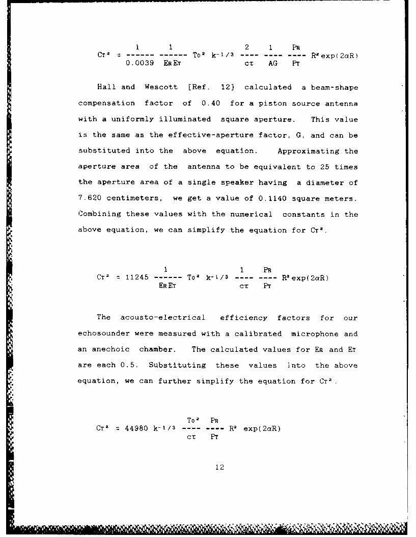
Hall and Wescott [Ref. 12] calculated a beam-shape

compensation factor of 0.40 for a piston source antenna

with a uniformly illuminated square aperture. This value

is the same as the effective-aperture factor, G, and can be

substituted into the above equation. Approximating the

aperture area of the antenna to be equivalent to 25 times

the aperture area of a single speaker having a diameter of

7.620 centimeters, we get a value of 0.1140 square meters.

Combining these values with the numerical constants in the

above equation, we can simplify the equation for CT'.

1 1 PRCT2 = 11245 ------ To2 k-1/3-------- Rlexp(2aR)

ER ET cx Pr

The acousto-electrical efficiency factors for our

echosounder were measured with a calibrated microphone and

an anechoic chamber. The calculated values for ER and ET

are each 0.5. Substituting these values into the above

equation, we can further simplify the equation for CT'

To' PRCT2 = 44980 k-1/3 R--------R exp(2aR)

c Pr

12

Id".

The above equation was incorporated into the computer

program that provides the system control, data acquistion

and data processing techniques [Appendix A]. The reduced

data was then used to measure the temperature structure

parameter as a function of time of day and altitude for

various sites.

13

III. SYSTEM DESIGN AND EQUIPMENT DEVELOPMENT

A. HARDWARE

Most of the hardware used in this system was standard

scientific equipment and is illustrated in Figure 1. The

Wavetek 852 Pre-amplifier iNBandpass Filter C

Computer O

Monitor isAD200 Analog U

to Digital RConverter E

HP 200 Seriesc erComputer Amplifier 5 X5 Speaker

Disc Drives System Arra

Computer HP3314AFunction

Printer Generator

Fig. I. Echosounder Equipment Arrangement

14

pieces which were specially designed by L T e ir--ir trni-

[-Ref. 31 are the acoustic array and the enclosure for thiF

array. The design considerations for the speakers and the

.array format are given in Appendix B and the desian Cif fh,-

frl-vlosure to house this array is -,utiined in Appendix (..

Aside from these two pieces of equipment, there Are

primarily six other components which comprise this

echosounder. Below is a brief description of each of these

additio-_nal components.

1. HP200OC Series-Computer

The Hewlett-Packard (HP) 200 Series Computer

tncludes a 20 megabyte hard disk drive, a floppy disk drive

and an associated printer arid monitor. The HP200 Szeries

Ci',mpute-_r was the central control component for the ent ir

eCho-_sourider arrangement. The computer used was an HP:.21i/

Pr,-)rammrnd in Basic 3.0 and equipped with an Tnfotek C'Y

LE= Fic t:o-mpi Ler and an Infotek FP2lO Floating ~C iri ti

A -te L-eratojr to enhance the speed of program execution. h

pr-gram lefined all parameters for the HP33j14A Fun-tion

3enrj'jrtrr as well as execute the trigger command %-hi 4Ih

pr duedthe echosounder transmitted acutcpuLse..-

mpnuter also received the data fro-)m the _acoust fic arrayv

th e rpre-amplifier, baricpass filter and analog to dii-ital

z~ie ~--.The cromputer thn n c-cnducted the data re-Ju-ti-

r:i r,~ to, proDduce a nd display a high res-iit i r,

m.-,F pht r ) r()f iI e

2. HP3314A Function Generator

The Hewlett-Packard (HP) 3314A Function Generator

was a multimode function generator capable of providing

sine, square and triangular wave functions as well as any

desired waveform ranging in frequency from 0.001 Hertz to

19.999 Megahertz. The HP3314A Function Generator was used

to supply a pulse of an integer number (usually 100) of

sinusoidal cycles of constant amplitude to the QSC Model

1700 Audio Amplifier. A constant frequency setting of 5000

Hertz was used for all data runs.

3. QSC Model 1700 Audio Amplifier

The QSC Model 1700 Audio Amplifier is a high power

amplifier which can supply 350 watts over an 8 ohm load.

This amplifier was used to boost the output voltage of the

function generator by a factor of 20 from 1.5 volts to 30

volts. The power supplied to each speaker in the array

during operation was then 37.5 wat'.s.

4. Pre-amplifier

The pre-amplifier was designed and constructed by

Walters [Ref. 13] to supply a gain of 1000 to the returned

signal and isolate the data acquistion components from the

transmitted pulse. The pre-amplifier may be thought of as

a safety and switching mechanism for the system. An LT

1037 and an LT 1007 Operational Amplifier were selected for

use in the pre-amplifier based upon their low noise

properties which were evaluated by physically incorporating

16

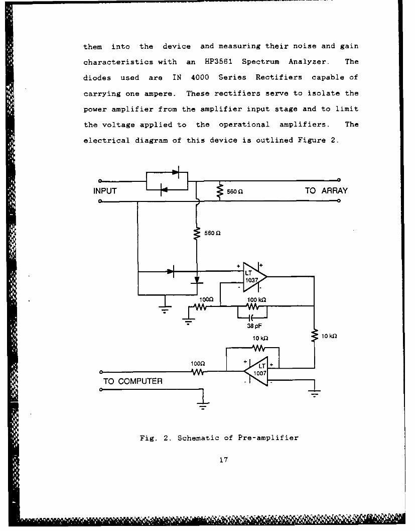
them into the device and measuring their noise and gain

characteristics with an HP3561 Spectrum Analyzer. The

diodes used are IN 4000 Series Rectifiers capable of

carrying one ampere. These rectifiers serve to isolate the

power amplifier from the amplifier input stage and to limit

the voltage applied to the operational amplifiers. The

electrical diagram of this device is outlined Figure 2.

INPUT 560 TO ARRAY- 0

560 £

+ L

J L° 1037

- 10000 k

38 pF

10k1 1 lk

~TO COMPUTER/

Fig. 2. Schematic of Pre-amplifier

17

5. Rockland Wavetek Model 852 Filter

The Rockland Wavetek Model 852 Filter operated as a

48 db per octave bandpass filter to suppress the broadband

noise of the system. High and low bandpass settings of

5500 Hertz and 4500 Hertz respectively were used. The

filter response at these settings is illustrated in Figure

3.

,START 1 888 Hz RAME! -5 OBV STATUS: PAUSED

A:MAG PMS:58-5

dBV

10 I

dlI/DIV

-85 1 iSTART: 1 880 Hz aW: 477.43 Hz STOP: 51 890 HzXs 5000 Hz Y:-29.24 dBV

Fig. 3. Bandpass Filter Response

The three db (half power) bandwidth is approximately I KHz

wide. Although it would be desirable to reduce the

bandpass to between 50 and 100 Hertz without impairing

signal response, the Rockland Wavetek Model 852 Filter was

18

the best filter available. It performed adequately in

spite of the large 1KHz bandwidth.

6. Infotek AD200 Analog to Digital Converter

An Infotek AD200 12 bit Analog to Digital Converter

was used to digitize the signal voltage for the computer

system at a 12.5 to 20 KHz sample rate.

B. SOFTWARE

The software and HP200 Series Computer system were

responsible for controlling and monitoring every

operational phase of the hardware components. The program

which accomplished this task was entitled "ACRDR" and is

listed in Appendix A. This program was modeled after a

program written by Walters [Ref. 13] but each program

performs a distinctly different computational task. This

program was written in HP Basic 3.0 and was compiled by an

Infotek BC203 Basic Compiler to enhance the speed of

execution.

The program "ACRDR" is easily broken down into a number

of blocks and subroutines which performed specific

operations. These sections are outlined in a flowchart

(Fig. 4). Each block is straightforward in its purpose.

and the program is designed to be as helpful to the user as

possible. As a prologue to the actual program code, there

is a listing of all the program variables with a short

description of their use. Such a listing familiarizes a

user with the computations to be made and also provides

19

i1 ji.....

quick references for any future modifications to be

implemented.

InitializationProcedures for:

HP 3314AAD 200 A/D ConverterInternal ClockConstants

uSend CT 2 Plot to the Compute Values of CT2

Computation of Printer and Plot

Parameters Tvarabe Speed of Sound

Range asth Pcot to tgPulse Length PrinterAttenuation Coefficient N Isthe Y

I- 15 Minute Pl

Complete?Prepare Screen forLData Display

oTrigger Pulse from Collect Return and jCompute the AverageHP31APerform Reduction Noise Level

~Routines, Store Data ifRequired

Fig. 4. Flowchart of Fundamental Program Operations

The initialization procedures which set all the

parameters necessary for data collection follow the

variable definition section. These parameters control such

things as the contrast between background and return signal

and the setting of the computer's internal clock. All

20

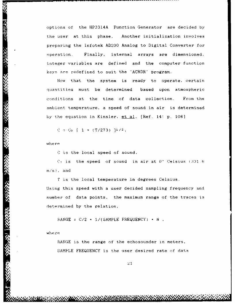
options of the HP3314A Function Generator are decided by

the user at this phase. Another initialization involves

preparing the Infotek AD200 Analog to Digital Converter for

operation. Finally, internal arrays are dimensioned,

integer variables are defined and the computer function

keys are redefined to suit the "ACRDR" program.

Now that the system is ready to operate, certain

quantities must be determined based upon atmospheric

conditions at the time of data collection. From the

ambient temperature, a speed of sound in air is determined

by the equation in Kinsler, et al, [Ref. 14: p. 106]

C z Co [ 1 + (T/273) ]/2,

where

C is the local speed of sound,

,- is the speed of sound in air at 0" Celsius V331.6

m/s), and

T is the local temperature in degrees Celsius.

Using this speed with a user decided sampling frequency and

number of data points, the maximum range of the traces is

determined by the relation,

RANGE = C/2 - l/(SAMPLE FREQUENCY) - N

whe re

RANGE is the range of the echosounder in meters,

SAMPLE FREQUENCY is the user desired rate of data

21V

acquisition, and

N is the number of data points per trace.

Typically, the values of many of the parameters are not

varied. The value of N above is almost always taken to be

the allowed maximum of 16301 data points and the speed of

sound can be -afely estimated to be 340 m/s at room

temperature. By using a typical sample frequency of 20000

Hz, a range of approximately 135 meters is obtained.

Another parameter determined is the atmospheric

attenuation coefficient. This calculation is done in a

subroutine obtained from Reference 15 and is necessary in

this program for the calculation of CT2. Other

computations made prior to program execution include the

pulse length, wavenumber, and the D-C offset of the

equipment.

At this point, the computer is finally ready for data

collection. The screen setup displays a distance versus

time plot and the internal clock of the computer is

synchronized with the pulse from the HP3314A Function

Generator. Following transmission of the pulse, the return

signal is received, digitized, stored in an array and data

reduction commences. A block averaging technique is used

in which a block of data points the size of the number of

emitted cycles is summed and averaged. Returns are plotted

:s darkened areas on the echosounder traces with the

intensity of the darkened area linearly related to the

22

|. .

-' .1 g 'lp ~ .~ ~ 4

magnitude of the return signal. This same procedure is

used in the computation of CT2 with some very important

differences. Aside from simply correcting for nr

spherical divergence, CT2 is corrected for electronic gain,

the ratio of power returned to power transmitted, the

efficiency of the speakers as transmitters and receivers,

the area of the speaker array, the atmospheric attenuation,

the pulse length, the temperature, the scattering cross

section per unit volume at a specific range and frequency

and finally the effective aperture factor of the antenna.

Additionally, CT 2 (Range) is averaged for a particular

altitude over 15 minute intervals. Finally, after each

pulse is reduced, a corresponding mean square noise level

, is determined. This is done by averaging each block

average at maximum range until at least ten values have

been used in the average. An upper limit of five over the

average noise figure (this corresponds to voltage

fluctuations on the order of lU- 7 volts) is set on the

routine to avoid averaging any strong return signals or

anomalies such as passing aircraft. After the ten values

are averaged, every subsequent pulse is averaged into all

the preceding noise levels and removed from each subsequent

return signal.

Ultimately, after e~ch 15 minute interval, or at the

users request, the display terminal image is printed. At

this time the T2 computations are conducted and plotted on

the screen and printer as range versus logio of CT2 . Upon

completion of the printing of these plots, the system

begins the data processing for the next 15 minute interval.

There are certain options built into the program to

allow a user to change various aspects of operation. The

function keys allow the user to change the lo,-a

temperature, sample frequency or intensity factor during

program execution. Additionally, the user can quit -r

restart the program, print the partial trace on the screen

or elect to save a trace on a floppy disc. The save

routine is invoked for the subsequent 15 minute interval

after the appropriate function key is depressed. Saving a

future trace may seem awkward, especially if a user would

like to keep an interesting trace which is presently on the

terminal. This problem cannot be readily solved unless

each trace is recorded to disc without us r intervention.

At present, this is not done because only 8 traces (2 hours

o ,f data) can be written to a floppy disc before it is full.

Z4!

IV. DA A ANALYSIS

A. ECHOSOUNDER PERFORMANCE

An analysis of the acoustic echosounder output was

conducted to determine the validity of previously

determined echosounder parameters. The e-1 decay time

constant for applied voltage was calculated in Appendix B

to be approximately 900 js or for convenience, 1 ms.

Reviewing typical echosounder traces and CT2 plots

[Appendix D], it was evident that the recovery time was

typically found to be on the order of 33 ms or roughly six

meters past the end of the transmitted pulse length of 3.4

meters. The recovery time is consistent with the time

required for the 30 volts on the drivers to decay to the

microvolt level. A more detailed analysis of the hardware

is found in Reference 3.

B. SITE EVALUATION

Echosounder data was collected at two different

locations. The primary data collection site was the upper

roof of Spanagel Hall at the Naval Postgraduate School,

Monterey, California. This site was chosen simply for

convenience. Data gathered at this location is believed to

represent the California coast during the spring near sea

level. The second site chosen was in the vicinity of the

24 inch telescope at Lick Observatory, San Jose,

25

California. This site is located atop Mt. Hamilton at an

altitude of approximately 5700 feet and nearly 20 miles

inland from the coast.

These two data collection sites represent areas of

differing atmospheric air pressures, water vapor pressures,

local temperature ranges, and local wind velocity ranges.

These characteristics all play important roles in effecting

the local atmospheric turbulent conditions and thereby the

atmospheric structure parameter, CT2 .

In addition to collecting echosounder data at Lick

Observatory, simultaneous measurements of the isoplanatic

angle (80) and spatial coherence length (ro) were made with

systems developed by Walters [Refs. 1 and 2]. A basic

knowledge of these two systems is necessary to understand

the correlation procedures made. The isoplanatic angle

(Oo) is primarily an upper atmospheric measurement which

indicates atmospheric disruptions at a range of 2 to 15

kilometers. The spatial coherence length (ro) is a measure

of the effects of the entire atmospheric blanket on

coherent light transmission. A close comparison of all

three data sets should give us an accurate description of

both the lower and upper troposphere as well as the

* stratosphere above.

Based upon isoplanatic angle (80) and spatial coherence

length (ro) measurements at Mt. Wilson in California, a

strong correlation between the two measurements occurs if

26

the low altitude boundary layer contribution is

sufficiently small. This strong correlation helps toreinforce the overall description of the atmosphere at the

time of data collection. Figures 5 and 6 graphically

illustrate the atmospheric measurements made at Mt. Wilson

on 2 April 1987 by Walters.

30 2 Rpril 1587 Mt Wilson28

i.2422

v 20

Ce-16u 14

-L2da 1.a @S8

- S(fil

CL04

0 O IL 0 2 IiTime (hr, U7)

Fig. 5. Isoplanatic Angle Measurements, Mt. Wilson

27

- - I.% I

2 Apri_ 1 1987 l Mt Wilson

4001

300

200I

a0d 4 a 10 1""1 16Tim (rsUT) 1Fig. 6. Spatial Coherence Length Measurements, Mt. Wilson

The strong correlation between the isoplanatic angle

(8o) and the spatial coherence length (ro) is especially

evident between the hours of 0700 and 1300 universal time,

The close tracking of these two measurements during this

time interval indicate that the upper atmospheric

conditions, as measured by eo, are dominating the entire

atmospheric profile as measured by ro. Unfortunately, the

existence or non-existence of any turbulent surface effects

cannot be ascertained by the employment of the above two

systems alone. However, employment of these two systems

28

-ha fil

together with the acoustic echosounder should enable us to

produce a complete atmospheric profile with strong

correlation between all three atmospheric measurements.

On 9 and 10 April 1987, all three systems were operated

at Lick Observatory. Again, a good correlation between the

isoplanatic angle (Go) and the spatial coherence length

(ro) measurements was noted. In addition, a strong

correlation between the spatial coherence length (ro) and

echosounder measurements was present. A comparison of the

atmospheric data in Figures 7 and 8 shows a good

correlation between the two parameters especially during

the 0930 to 1130 time interval on 9 April 1987. However,

during subsequent hours the isoplanatic angle (6o)

Ameasurements remain high (-12 4rad) indicating relatively

calm turbulent conditions in the upper atmosphere while the

spatial coherence length (ro) values drop sharply after

12:00 Universal Time indicating dominant and increasing

lower atmospheric turbulence. This increase in the low

level turbulence should be evident in the echosounder data

commencing around 1200 universal time (0400 local standard

time) on 9 April 1987. A comparison of the echosounder

data in Figures 9 through 11 illustrates this increase in

the local surface turbulence.

29

20 9 Aprt1 1997 Lick

12

C l6

14

CI

'0

2

10) II 1-3 13 1

,I=Time (hrs UT)

Fig. 7. Isoplanatic Angle Measurements, Lick Observatory

300 9 April 1987 Lick

200

2

0

100

i I i I , I , l i | .

07 8 3 10 11 12 13 14

Time (hrs UT)

Fig. 8. Spatial Coherence Length MeasurementsLick Observatory

30

-, , ....,.. .. .... .. . , , .., .. .. ., ,....... ..- : :, y , .--. , .,_ . . - -, ' ", -

9 Apr 1987 LICK OBSERVATORY135

~90LLI

L... .......~

3:00 3:05 3:10 3:15

Fig. 9. Echosounder Trace, Lick Observatory

9 Apr 1987 LICK OBSERVATORY135

se--

Li -

4!00 4-05 4!1.0 4!15

TIME LOCA-L (S7D)

Fig. 10. Echosourider Trace, Lick Observatory

31

9 Rpr 1987 LICK OBSERVITORY135

U. . . .. . ...., '.. ...... - . . .. .... . . "..[ '..:: . . -,. ...... i :".i " :!:.

... ... ... ..

U'l

v A.

TIE OAL(SD

Fig. 11. Echosounder Trace, Lick Observatory

The strong correlation between the echosounder data around

4:00 to 5:00 Standard Time and the ro measurements around

12:00 Universal Time combined with the lack of correlation

between the Go and ro measurements indicate that the lower

atmospheric and surface turbulence are dominating the

atmospheric profile during this time period.

Data collected on 10 April 1987, again illustrate the

strong correlation between the three atmospheric

measurements made. A comparison of the Go and ro

measurements during the time interval of 0700 and 1300

Universal Time indicate steady turbulent conditions in the

upper atmosphere and greatly varying turbulent conditions

32

S.: . . . i; • ':. .. : . . . "

at lower atmospheric levels. This is evident in Figures 12

and 13 by Lhe consistent values of 9o during the time

period compared with the steady increase and eventual

decline of the ro values during the same time interval.

The trace variations in Figure 13 during the hours of 0800

and 1200 are indicative of a period of decreasing lower

atmospheric or surface turbulence followed by the onset of

an increasingly turbulent period around 1200. This

turbulent trend is strongly supported by the echosounder

data in Figures 14 through 21.

:20_ 1.0 Rri 1 137 Lick

~18L3 6

14

cL 6 E L [

-8 81~ f10I 14

Tme (hrs UT)

Fig. 12. Isoplanatic Angle Measurements, Lick Observatory

33

300 10 Aril 1987 Lick ___

200

6.f

1006K

4610 12 14Time (hrs UT)

Fig. 13. Spatial Coherence Length Measurements,Lick Observatory

10 Rp 1987 LICK OBSERVRTORY135

LI a

Lij

00-00 0-05 0!10 0:15

TIME LOCAL (SiT)

Fig. 14. Echosounder Trace, Lick Observatory

34

"'l" P 11 *.* 'I

13510 Apr 1987 LICK OBERVATORY

U90

U

4-j

1 !00 1 !05 1 - 1 1-15

TIME LOCAL (STD)

Fig. 15. Echosounder Trace, Lick Observatory

10 Apr 1987 LICK OBSERVRTORY135

z

L 4 .Ji %

10 Apr 198? *LICK~ OBE:z-RVRTORY

902La2i521021

I J.

0 . . ......-------- -- --

2!00 2!05 2:10 2:15TIME LOCRL (STD)

Fig. 18. Echosounder Trace, Lick Observatory

1336

- L% n- . ~ ..

10 Apr 198? LICK OBSERVRTORY

11*5

U .

Li 90Li

-w1-Al'

0 .... .... . ...

3:30 3:35 3:40 3-45

TIME LOCAL (STD)

Fig. 19. Echosounder Trace, Lick Observatory

10 Apr 198? LICK OBSERVRTORY

7 .p.0 ... . .*

. I.

~~4:i ...40 4:0 4:0

377

Fig.~ ~ ~ ~ 20 Ecoo e Trace, Lic Oberatr

~~37

C .t

10 Apr 1987 LICK OBSERVATORY

90

135

0 . ....• .. . . . . ; . " . .

4-04 5 ' 4:4 4:45

TIME LCL (S7-

9 0 4... ...... 4:40 ... ,....

Fig. 21. Echosounder Trace, Lick Observatory

The large 200mm coherence lengths around 11:00 Universal

Time are consistent with the low turbulence evident in the

echosounder profiles around 3:00 Standard Time followed by

a pre-dawn increase in the surface turbulence.

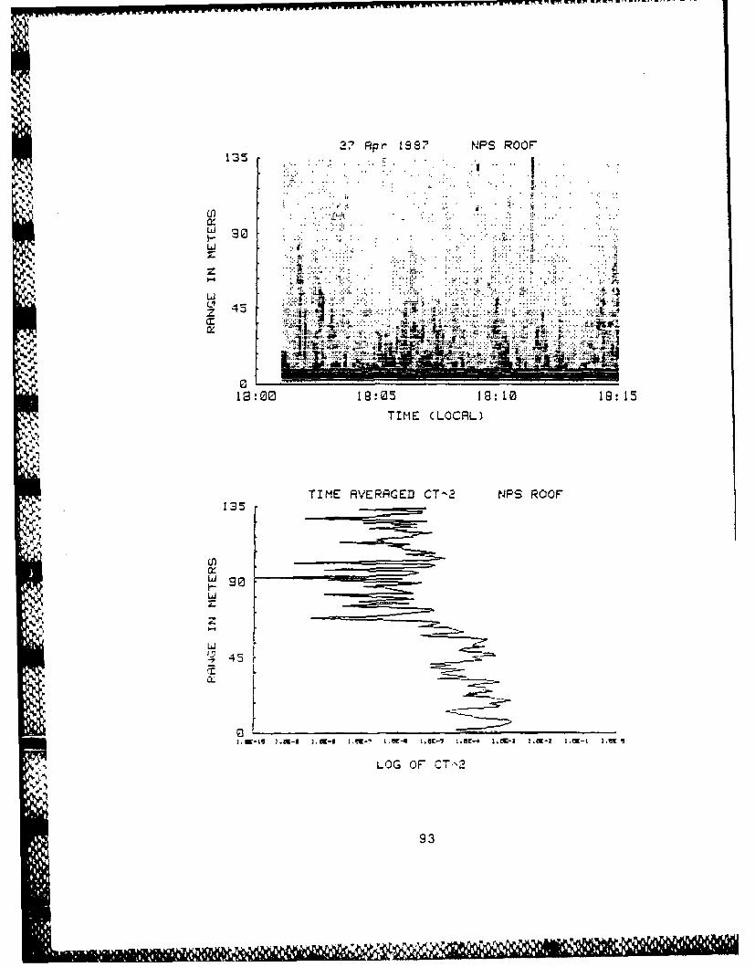
Only acoustic sounder atmospheric measurements were

made on the upper roof of Spanagel Hall at the Naval

Postgraduate School. Data runs on 26 and 27 April 1987,

included both echosounder data and the associated C T2

plots. A representative sample of the data collected

during this period is included in Appendix D. Of

particular interest is the data in Figure 22, which shows

the maritime boundary inversion layer at about 100m and

being perturbed by convective plumes at lower altitudes.

38

................ ........ .,............................

27 Apr 1987 NPS ROOF

-~A A. L.

. 4rm :Y1.

C M 301.~1 .,i- 4 2;;~- 'I-~ **-~ .- -~ ~ *~*-

n.- - - .

44

LOIME (LC-2

Fi .3 2. Ec os un5 Trace andPG~ CT- P lot ROORoo

JL

L39

V. CONCLUSIONS AND RECOMMENDATIONS

A high frequency (5KHz) phased array echosounder

constructed to measure low level turbulence appears to work

within the 10 to 135 meter altitude range. When using the

device, detailed profiles of the short range atmospheric

density fluctuations were obtained. The profiles were

found to correlate very well with the measurements of the

isoplanatic angle (0o) and the spatial coherence length

(ro) during periods of simultaneous operation. This short

range echosounder, when used in conjunction with the other

atmospheric measuring devices, is an invaluable tool. The

graphical output provides us with a more complete

description of the atmosphere that can be used to calculate

Cn2 , the atmospheric index of refraction structure

parameter.

Further software development such as the incorporation

of Fast Fourier Transform routines into the echosounder

program will determine the radial velocity profile of the

return signal. Such an improvement will determine the

velocity of the probed air masses and plot these

echosounder traces as a function of color intensity.

Other areas of further reasearch include the design and

testing of different array patterns. One such pattern, the

hexagonal array, is already undergoing tests. As the

4 0

speaker array evolves, it is also evident that the

enclosure must follow suit to accomodate the new array

design and associated beam patterns. Further improvements

in software routines are also inevitable. It is always

desirable to store on a disc all data collected at a site.

Presently, the floppy disc capacity is inadequate for the

storage of more than two hours of data. Furthermore, if

FFT and Doppler routines are to be added, the computational

speed of the computer will inhibit the pulse repetition

rate. A special data acquisition technique called "Direct

Memory Access" may then have to be introduced into the HP

computer to allow simultaneous data collection and

processing.

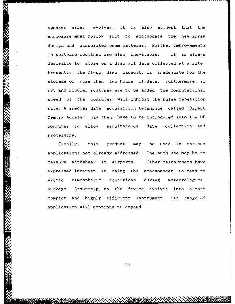
Finally, this product may be used in various

applications not already addressed. One such use may be to

measure windshear at airports. Other researchers have

expressed interest in using the echosounder to measure

arctic atmospheric conditions during meteorological

surveys. Assuredly, as the device evolves into a more

compact and highly efficient instrument, its range of

application will continue to expand.

41

APPNDIX-A

ACOUSTIC ECHOSOUNDER PROGRAM

20 i ACRDR *

30 ' COMPUTER SOFTWARE WRITTEN BT LT. M. WROBLEWSKI FOR AN *

40 1 ECHOSOUNOER BUILT FOR A MASTERS OF SCIENCE THESISso 1 BY LT. M. WROBLEWSKI AND LT. F. WEINGARTNERGo * ADVISOR: PROF. D. WALTERS70 'JUN. 1987

110 1 The computer program receives information from an acoustic120 1 array through an A-D converter. This information is the130 1 returned signal of an acoustic pulse as it passes through140 1 the atmosphere. The data is then used to display the returnISO I intensity with distance as a function of time. This is a163 1 short range device (from ISOm to 200m).170180 I190 1 LIST OF VARIABLES

210

2 I I & K & J - counters for loops230

240 Rec-num & Nrec - real and integer representation of the250 record number for storage

270 Plotnum - counter used to insert form feeds between plots290

I isc-address$ - storage location of data file

S le$ file nar-e Ased to to-e data

I "T. ,. - tr. g and , a=I rec,-esent t , of "he n ,iber ofcycCes and tte IeC of nt5 ,j5 d 1r the

computation of the block average

370 Point(*) real number representing the noise and range300 $ corrected average over given number of points

40 Cat%') array of a-d converter output after sampling4104

42

&42 1 020) - array of reduced and averaged data including430 1offset, correction for noise, arid range440 Icorrections450460 Hrs - the integer hours470 1480 Min - the number Of Minutes

490500 Qtrhr &Qtrmin - keeps track of the passage of each510 IS1 minute interval5ILO I530 1 Numi counter for computation of block averagesS40S50 1 NumZ counter for the number of block averages made5GO I570 ! M - the counter used in the plot label routinesSoo0S90 ! Timont -- time interval between data sample in600 i nanoseconds6;10 16203630J I~max -total number of block averages computed640650 IFreq$ Freq - the frequency input of the HP3314A in kilohertz660670 Zone$ the appropriate time zone the operator desiresGOO690 ISite$ the name of the appropriate site of data collection700

71 I Zaveplt &Cntrl - on/off toggles used to determine whether72Z a particular run will be saved to a disc7 3074Z Nplot -the number of increment along the entire7"ISO horizontal axi5

770 Offset -the computed 0-C offset for the system prior700 to data acquisition

7 00SOO io i ae -a running total of tlhe -cse ac:zrmulated a, the

rla,*uIMIr -ageuez; to fi:- ar., rer tra£22O avei-age nose

040 Lmit -the upper bound on the noise figure used to insureGGIV that large returns are not included in theG 86 noise computations370830 111 a counter of the number of traces used to determine890 the noise average

43

wu* r.

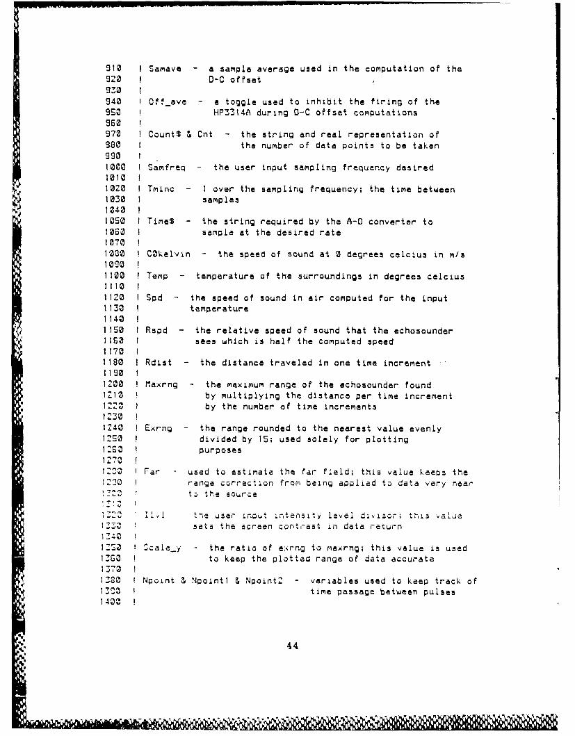
910 1 Samave - a sample average used in the computation of the920 1 D-C offset930

940 Offave - a toggle used to inhibit the firing of the950 HP3314A during D-C offset computations960970 1 Count$ & Cnt - the string and real representation of980 I the number of data points to be taken9901000 Samfreq - the user input sampling frequency desired10101020 Tminc - 1 over the sampling frequency; the time between1030 1 samples1040 11050 Times - the string required by the A-0 converter to1060 sample at the desired rate10-70

00 COkelvin - the speed of sound at 0 degrees celcius in m/s10001100 Temp - temperature of the surroundings in degrees celcius11101120 1 Spd - the speed of sound in air computed for the input1130 temperature114011S0 I Rspd - the relative speed of sound that the echosounder1160 1 sees which is half the computed speed1170 11180 Rdist - the distance traveled in one time increment1190 !1200 Maxrng - the maximum range of the echosounder found1210 by multiplying the distance per time increment1220 by the number of time increments12301240 Exrng - the range rounded to the nearest value evenly1250 divided by 15; used solely for plotting12I purposes1270

1230 1Far - used to estimate the far field; this value keeps the1220 range correction from being applied to data very near

to the source

I3S3 Z II 'he user input intensity level diiscr; this va'Le133 sets the screen cont,-ast in data return134 0

1icale_y - the ratio of exrng to maxrng; this value is used1360 to keep the plotted range of data accurate13701330 Npoint & Npointl & NpointZ - variables used to keep track of1390 time passage between pulses1400

44

1410 T2 & TI & TO - used to synchronize data collection with the

142 clock

1430 1

14430 TIMEDATE - the internal clock of the computer

14SO 11460 Ovd - divisor of the data average; used because computer

1470 multiplication is faster than division

14301490 R - the range of a block of data samples

1S0ISTO Run-ave - the running sum of the block samples

1520

1530 1 X - the value of the data point less the 0-C offset

1540 11550 ! Ns - the final average of the block of data points; also

15EG i used in the computation of the noise figure

1570

IS80 Corr - the noise correction applied to the data samples

1530

1600 1 Time - the horizontal position of the trace on the plot

1610 1

1620 1 Timedist - the horizontal width of the trace on the plot

163G !

IG40 Endpt - the last point of the plot vertically taking

165 G into account the scaling factor scale_y

IG6

1G670 Inc - The vertical increment along the plot

I1S I

1G69 I Z - The final reduced data points which are output on the plotS1700

1710 Dis - The vertical height of the trace on the plott 1720

1730 0 Ap$,Frq$,Nm$,En$,Vo$,Hz$ - strings needed to set the HP3Z14A

1713

17G Amp$ - userv input amplitude for the HP3314A

17 GO1770I Plsng - the pulse length of the burst

17 0 Ct( - the atmospheric temperatue structure parameter

i '2 Y 'he nu, e t,-ae:-35n czr C t n C

p - the vertical poit~o on the Ct plot

1SO I Pnt- the horizontal positlori on the Ct plot

1370 3 - the wave number to the 1/3rd power

1O023 A The area of the receiver (array)

45

1310 1 G -The effective aperatu.re factor

1930 Er -efficiency of cover-sion of acoustical power1940 Ito electrical power on the recieve side

1360 IEt -the efficiency of conversion of electrical13970 power to acoustical power on the transmilt side13201030 Pt -The computed transmitted power to theZ0 W 0 acoust ic arrayZ20t1021020 1 Gain - the electronic gain of the equipmentZ2Q0Z0 1"040 IZimp - the speaker array impedence

2020 OPTION BASE 1

200

A.110 Iinitialize the arrays S set dimensions2120 1 declare all integer variables

2140I41SIZ DIM Disc-addrass$EC20J,File30,Point(00),Ct(200)2160 INTEGER I,Hr ,Plotnum .Print key ,Num,Numl *Num2&,M.K

210 INTEGER Rac_num,Kmax210 INTEGER 0(0)Ot 61)BUFFER

2 I initialization routines.... .set time, set HP3314A Function2220 1 Generator

22402Z53 Rstrt:'iLL Fr-eq initsFraqS,N$)

2260 CALL Init-ad2'002270 CALL Set-time(Zone$)2233 LNPUT "GaLTE NAME ,ia

23:0 keyboard set _,p - sts labals on the camputer- furiction2340 keys

230OUTPUT KBO;'SCRATCH KEYE ; CLEAR THE KEYS2."80 CCN T RO0L 22 ; IZ',30 ON KEY ILABEL "NEW TEMPI GOTO Speed

46

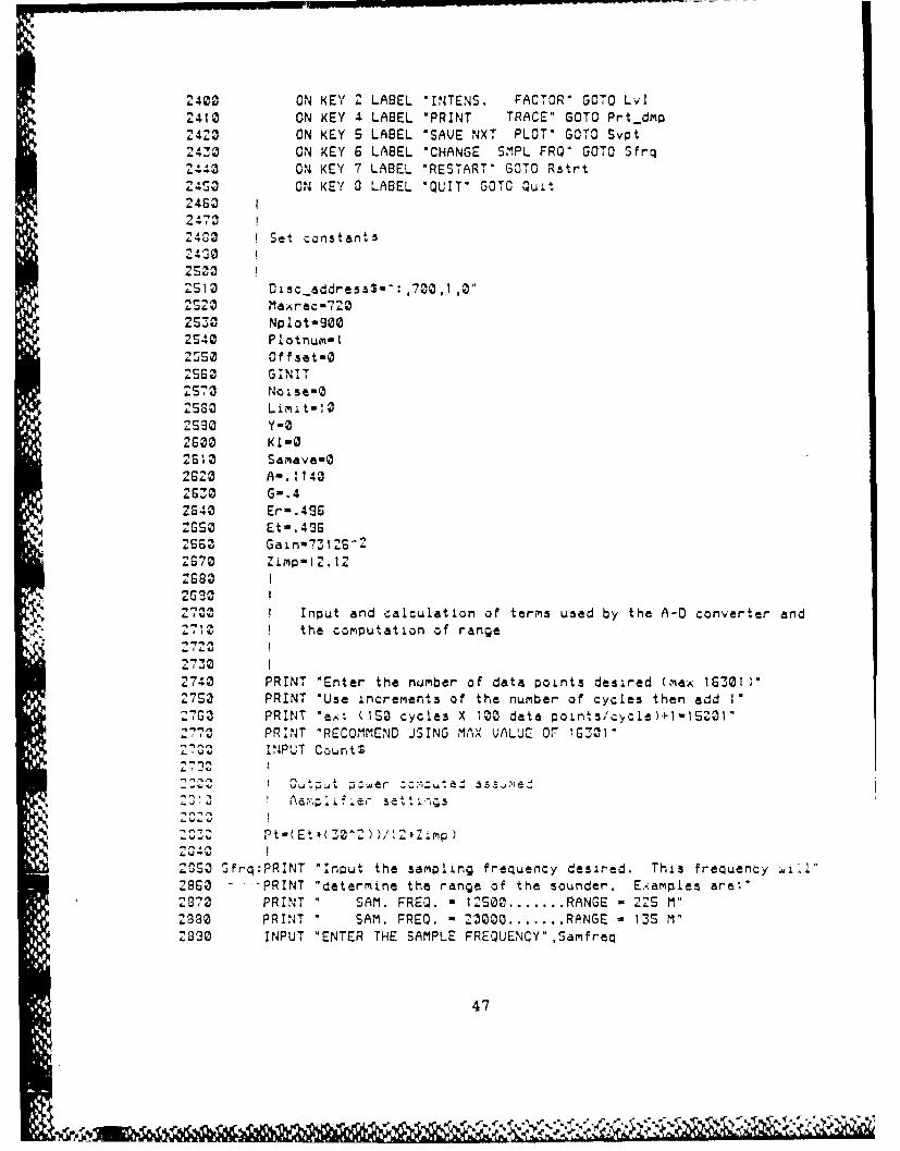
2400 ON KEY 2 LABEL "INTENS. FACTOR" GOTO Lvl2410 ON KEY 4 LABEL "PRINT TRACE" GOTO Prt-dmp2420 ON KEY 5 LABEL "SAVE NXT PLOT" GOTO Svpt243 ON KEY 6 LABEL "CHANGE SMPL FRO' GOTO -frq2.44 ON KEY 7 LABEL "RESTART" GOTO Rstrt2450 ON KEY 0 LABEL "QUIT" GOTO Quit2463 I2470

4.40 i Set constant524302500 i

2510 Oisc addres$S':,7OO,IO"2S2 Maxrec-7'02530 Nplot-9002540 Plotnum-I2550 Offset-O25G0 GINIT2570 Noise-O250 Limit-102690 Y-O2600 KI-O2G10 Samave-O2620 A=.1i40263G G-.42S.10 Er=.496ZGSO Et-.4962660 Gain-7312 G".2670 Zimp-12.12

Z683ZG302700 I Input and calculation of terms used by the A-D converter and2710 the computation of range2720

2730

27.40 PRINT "Enter the number of data points desired (max 16301)"2750 PRINT "Use increments of the number of cycles then add 1"27G0 PRINT "ex: (ISO cycle3 X 100 data point5/c~cle)+1-ISQOl"2770 PRINT "RECOMMEND JSING MAX VALUE OF IG301"270 IPUT Count$

2720

2050 'Frq:PRINT "Input the sampling frequency desired. This frequency wiil"2860 -- PRINT "determine the range of the sounder. EXamples are:"2370 PRINT " SAM. FREQ. - 12500 ....... RANGE - 225 M"2980 PRINT " SAM. FREQ. - 23000 ....... RANGE - 13S M"2330 INPUT "ENTER THE SAMPLE FREQUENCY",Samfreq

47

2900 GCLEAR239,10 Tminc- ./SamfreqM9d0 Timcnt-1000*INT(Tminc/I.E-G)2930 Time$-"TIME "&VALS(TiMcnt)2940 Cnt-VAL(Count$)29SO COkelvin-33 1.G2g63 Num=VAL(N)237Z Freq-VAL(Freq$)*I0002930 I

UV I Computation of the O-C offset prior to program run300iz3020 I

3030 Off.ave-I.304 0 Offset-030S0 FOR I-I TO 10300 CALL Read-ad'00(Oat(*),Count$,Time$,Off_ave)3070 FOR K-I -0 (Cnt-1)3030 Samave-Samave+Dat(K)3090 NEXT IK3100 PRINT "COMPUTING D-C OFFSET"3110 NEXT I3120 Offave-03130 Offset-Samave/(10*(Cnt-1))3140 PRINT 'OFFSET IS :",Offset31S0 !31G0 I

3170 I computation of the speed of sound at a given temp and the3180 I range of detection of the device3190 13200 I3210 Speed:INPUT "Enter the temperature (celsius) ",Temp32:0 Spd-C~kelvln*(SQR(I+(Temp/273)))3:3 Ps pd-Spd/A"3240 Rdist-Tminc*Rspd326G Maxrng-Cnt Rdist320 Exrng-((INT(Maxrng'30))+.S).Z0.0

327 Far-Il.l(Tminc'Spd)

Z2ro Lambda-Spd/FreqK &(2aPI)/Lambda)^ 'I"-, , -, C,

3340 PRINT "Enter the relative intensity division level. This"33.0 PRINT "value is used to determine the plot intensity by3360 PRINT "dividing the block average sum by this number."3370 PRINT "This value is dependent upon the gain of"3330 PRINT "the device and will probably need adjustment"3390 PRP4 T "during run. Start with a value of about 4000"

3400 PRINT Pt

48

pis

3410 Lvl: INPUT Ilv!3423343 0

3440 set up the plot

3470 Again:CALL Plot-setup(Nplot,Site$,Maxr-ng.ScaleyExrng Zone$)3480 Nr-ec-0

34G0 FOR 1-1 TO 200

3310o NEXT I

3530 Npoint 103S40 OUTPUT KBD;*L~l3550 1

3'273 Sync: Isynchronize data collection with clock3583 TI=INT(TIMEDATE MOO 86400)35930 IF T1<TZ THEN TO-TO-86400.36 IF Tl-T3(1 THEN GOTO Sync36G10 TO-TI36270 1

3640 1 Data collection and reduction

3660 I3670 Read slg: Iread the A-0 converter3683 CALL Read-ad2'00(Dat('),CountS,TimeS,Off_eve)3690 Npoint-INT(TI MOO 3600 1100 Nplot)3700 Npointi2-Npoint-Npointlj I3710 Numl-Num-1

3720 Nu2=Cnt-Num3730 vd-I./CNum)

3770 FOR I-1 TO NumZ STEP Num'3780 R-I*Rdist

*3730 IF I<Far THEN R-1

K =K + I

F~~JI TOQ I ;Nu m I.4. --- SX=Cat~j)-Cffset

3042 Run-ave-Run-ave+X'X3350o NEXT J3860 N5-SQR(Run-aveeOvd)3870 Point(K)-R*(Ns-Corr)3.830 IF KI>10 THENZ390 Ct(K)=Ct-(K<)+((Point(K)^Z);EXP(2"-R*Atten))

3200 Ct(K<)-(Ct (K )*((3.339E-8 )^')'Er )/Zimp../J10 END IF

49

3920 IF Poant(K)>ABS(32767) THEN Point(K)-327673930 D2(K+10)-INT(Point(K))3340 NEXT I3950 IF KI110 THEN3360 Y=Y+I3970 END IF3390 I

4000 1 Noise correction routine4010 14020 !4030 IF Ns<(Limit+S) THEN4040 Noise-Noise+Ns4050 Kl-KI+t4060 IF KI1I0 THEN4070 Corr-Noise/Kl4080 Limit=Corr4090 ELSE4100 Corr-O4110 END IF4120 END IF413041404150 1 Plotting of the data416041704180 Kmax-K4190 REDIM D2(Kmax+IS)42004210 ! positioning the data on the plot by time of trace4220 14'30 Time-(Npoint2/Nplot)*404240 Timedist-L+((Npoint2+Npointl)/Nplot)'4204250 IF Npointl-O THEN Time-S4260 IF Npoint<6 THEN Timedist=G4270 End-pt-Scale y'2604280 D, 2 )=Kma.x4230 02(3)-INT(Temp)430 02( 4 )=INT( Time )431 02(- )=INT( Timedstw 10)-3-0 WINDOW 0,420,0,250

4330 GRAPHICS ON4340

4350 ! set the vertical increment4360 i4370 Inc-((Num*Tminc*Rspd*Endpt)/Maxrng)4380 2(6)-INT(Inc*1000)4390

50

We

4400 I compute the intensity of the return, move to the proper4410 I coordinates and plot the appropriate colored block

4420 14430 FOR K-I TO Kmax

4440 Z-Point(K)/Ilvl

4450 IF Z>1 THEN Z-I4460 IF Z<3 THEN Z-e

S44-70 AREA INTENSITY Z,Z,Z

4400 Dis-INT(KInc)+l4490 MOVE Timedist,OiS4500 RECTANGLE Time,Inc,FILL

4510 NEXT K4520 14530 I keep an account of the trace numbers taken on the plot4540 I4550 Nrec=Nrec+l

4560 Rec-num-INT(Nrec)

4570 D0.( 1 )-Rec-num4G80 Npointl.Npoint4590

4600 14610 I save routine - if function key is set then4640 1 the plot will be saved

4630 14640 1

4650 IF Cntrl-1 THEN

4660 ASSIGN @Filel TO Filel$4670 OUTPUT @Filel,Recnum;O2(*)

4680 ENO IF4690 I

4700 I

4710 I graphics dump of plot after 15 minute intervals

4720 1

4730 4740 IF Timedist)415 THEN

4750 Prt-dmp: PRINTER IS 701, 47G3 PRINT " "

4770 PRINT "

47C2 PRINT "

400, 0,UI, GRAPHICS 47014010 FOR TVi TO I';,ax4 0-0 C t (I)=-C t I (Temp 4'73 Z 2)( .0.3 2 ,K3,(t.,"I(

4.30 Ct(lI)Ct(I)'(I./(A'* ))4040 Ct(l)-Ct( I)*(./Pt)4850 Ct(l )=Ct( I )/Plslng4060 IF Ct(1)<l.OE-r00 THEN Ct(I)=I.0E-100

4070 NEXT I4000

51

4900 CT^Z ComrPutdtion3 and Plot5

4 9204930 GCLEAR4940 VIEWPORT 19,120,19,804950 WINDOW 0,300,0,EArng4960 AXES30Ern/S003,ag/4370 CLIP OFF

44980 OSIZE 1.64990 LORO 6S030 FOR lM0 TO 300 STEP 309010 MOVE M,-Exrng/4S5020 LABEL ".E;(/0-05000 NEXT M9040 MOVE 140,-15So50 CGIZE 49060 LABEL "LOG or T250170 LORG 85-080 FOR M-0 TO E;.xng STEP INT(Exng/3)5090 MOVE 0,M5100 LABEL M511o NEXT M51,20 LOIR P1/Z9130 LORO G9140 MOVE -40,Exrng/'29150 CSIZE 49160 LABEL "RANGE IN METERS"5170 LOIR 05180 LORG 49190 MOVE 150,Exrrng+35200 LABEL "TIME AVERAGED CT^2 .,Site$92-_10 CLIP ON9220 MOVE 300,09230 FOR I-I TO Kmaxr9240 Ypl-(Maxrng/Kmax )*I5S6se Pnt-(LOG(Ct (I ) /2.302909E;1 )+10912 c0 IF- Pnt>i0 THEN Pntin?0. 27-0 IF Pnt(0 THEN Pntin0520 PntmPnt*-30S-223 DRAW Pnt ,'(pl9300j NEXT ISZ10 DUMP GRAPHIC. #701920l PRINT

9330 PRINTER ISj C'RT9340 GCLEAR5390 KI-10

9360 Limit-Corr5370 N4olse-10*Corr

52

5380 IF Cntrl-l THEN5390 ASSIGN @Filel TO aN5S400 END IF5410 Cntrl=O

5430

5S40O5450 ifsar the Plot is toiinbe saldthfiescrad

54605570

S480 IF Save..plt-I THENS490 CALL File_init(Oisc_addres5$,Nrec,Filel$)SS0O Save_plt=0

5580 Cntrl-i55:0 END IF5530S540

5550 start the next tS menute plotS563

,- Q S570

5580 GOTO AgainS570 END IF

5700 !

Q 5620 next trace2 58630

5740 aSS GOTO SyncSGBo

5730

570 N

57005710 Svpt: Save_plt-IS720 GOTO ReadG!g573Z5

S 7 '* 0 1~~*; ~~Y 'K

57'0 comp'etion routine

57'4" 'Wut:iS-100 ENO

GOO0 SUBROUTINE SECTIOIN

53

G33 SUG Freqinit(Freq$.N$)6040

6Ss f SETUP OF THE HP3314A~ FUNCTION GENERATOR6070 160806090 Ap$S"AP"6100 Frqt-*FR*G110 Nmw$u"NM*6120 EnS-s'EN"6130Ij Vo$-VO"6140 Hz-*KZ*GISO INPUT 'FREQUENCY DESIRE0 (kHZ) (S RECOMMEND)",Freq$6160 INPUT *AMPLITUDE DESIRED (V . I.SV MAX) *,Am~p$6170 IF VAL(AmpS)>1.5 THEN61803 Amp$S'1.5"6190 PRINT "AMIPLITUDE OF FUNCTION GENERATOR IS 1.5 V"620e END IF6210 INPUT "NUMBER OF CYCLES PER BURST (INTEGER) (10 RECOMMENDED)-,Ns6220 OUTPUT 707;*M036210 OUTPUT 707;*SRV26240 OUTPUT 707 ;Ap$&AmpS&Vo$&FrqS&Freq$&Hz$&NmS&NSEnS6250 SUBEND6260 1

6280 16500 SUB Init-adZOO

6520!6530 IINITIALIZATION OF THE A-0 CONVERTER654065s06560 Ad 5et code-17

6:730 WRITC1O (d-se1..soda,0;0GISJO LCNTROL Ad-3al-cde,0;16600 SUBENO66136620 16630

54

7000 SUB Set time(Zone$)7010 !7020 I7030 1 SET THE TIME DATE RECORDER7040 I70507060 PRINT "WHAT TIME REFERENCE ARE YOU USING? INPUT:*7070 PRINT " I FOR UNIVERSAL TIME"7080 PRINT " 2 FOR LOCAL TIME*7090 PRINT * 3 FOR YOUR OWN CLASSIFICATION'7100 INPUT K7110 IF K-2 THEN7120 Zone$-*(LOCAL)"7130 ELSE7140 IF K-3 THEN7150 INPUT *WHAT IS YOUR TIME REFERENCE-,Zone$7160 ELSE7170 ZoneS-"(UTC)7180 END IF7190 END IF7200 IF TIMEOATE<DATE('14 AUG 1984") THEN7210 INPUT 'ENTER -00 MMM YYYY*'',Date$7220 INPUT "ENTER "'HR:MIN:SC-',TimeS7230 SET TIMEDATE OATE(OateS)+TIME(TiMe$)7240 PRINT OATES(TIMEDATE),TIMES(TIMEOATE)7250 Tstart-TIMEDATE7260 TOTstart MOO 864007270 END IF7280 SUBEND7205

55

7SOO SUB Read-ad2O(INTEGER Oat(*) SUFFER,CountS,TimeS Off_ave)

7S30 1INFOTEK A-0 ROUTINE SET UP FOR EXTERNAL TRIGGER7540 17550 I7560 Ad-sel..code-1l7

7S70 I7580 !INITIALIZATION OF THE A-0 CONVERTER75907600 OUTPUT Ad-sel-coder"RESET"7610 OUTPUT Ad-sel_code;"INTERNAL','COUNT "&CountS,"HOLDON"7620_' OUTPUT Ad-aelcode;*ELAYON','SELECT 151 ends ,Time$7S30 OUTPUT Ad-sel-code;*STATUS"7640 ENTER Ads5e.code;Resp$7650 IF RespS ----------- THEN7660 ASSIGN @AdZ00 TO Ad-5el-code;WORD7670768e I triggering of the HP3341A76907700 IF Off-ave-0 THEN7710 TRIGGER 707'7'&Z END IF7730 ASSIGN @Buf TO BUFFER Oat(*)7740 TRANSFER @Ad2100 TO @Buf;WAIT7750 OUTPUT Ad_3elcode;*77G0 OUTPUT Ad_sel-code;*STATUS*7770 ENTER Ad-sel-code;RespS7780 IF Resp$<-*-----------THEN7790 PRINT 'ERROR- ;RespS7800 END IF7310 ELSE7328 PRINT "ERROR DURING INITIALIZAT ION =;Resp$

END IT-i 'w UG END

56

8000 $S Plot_setup(Nplot,Site$,Maxrng,ScaleyExrng0 Zone$)8010 18 020 i8030 SET-UP OF THE TIME PLOT 0N THE CRT804080508060 Scale..yiMa;rng/Exrng8070 GRAPHICS ON8080 LINE TYPE I8090 VIEWPORT 15,120,15,808100 WINDOW 0,Nplot,0,Exrng811e AXES Nplot/15,Exrng/lS,0,0,Nplot/3,Exrng/38120 CLIP OFF8 130 CSIZE 4,.S8140 LORG 681so TI-TINEDATE MOD 864008l6o Hrs-T1 DIV 36008170 TZ-TI MOD 3600a18o MininT2 DIV GO81930 Otrhi--Min DIV 158200 FOR M-0 TO Nplot STEP INT(Nplot/3)8210 MOVE M,-Ex,-ng/45

8228 QOtr-rin-QtrhrIS+(M*3/Nplot )'*8230 IF Otrmin6GO THEN8240 Qtrmin-O8,250 Hrs-Hr5+18260 END IF8_47Q LABEL USING D.OA,ZZ-iHrs;*:"1trmnn82030 NEXT M8290 MOVE Nplot/26,-158,300 LABEL "TIME "&Zone$83108320 1 LABEL ORDINATE8330I8340 LORG 38350o FOR M-0 TO Ex,-ng STEP INT(Exi-ng/3)83G0 MOVE O,M83710 LABEL Mi03 00 NEXT M0300 LOIR PI/23480 LORG G0410 MOVE -Nplot/"7,Exrnc;/f'8420 LABEL "RANGE IN METERS"8430 18440 ! TITLE8450 19460 LOIR 08470 LORG 48480 MOVE Np~ot/2.,Ex<rng+3

57

8490 LABEL DATE$(TIMEDATEY;' ";SiteS'8500 CLIP ON8510 SUBENO8S20 18530

8S40 I9000 SUB Attenuation(Freq,Temp,Atten)90109020

9030 This subprogram calculates the attenuation of the9040 1 sound in air based upon equations in Neff 197S90S0 1 (source of subroutine: Thesis of R. Fuller)9080

9070 I Variables

9080 19090 1 Atompres - input atmospheric pressure in mb9100 I9110 1 Atten - attenuation coefficient of acoustic wave9120 i9130 Att_max - Variable in program. It is the attenuation9140 1 at the frequency of the maximum attenuation91S0 I for the given input conditions.9160 1

9170 ! F - Ratio of the frequency to frequency at maximum9180 1 attenuation.

S9190I9200 Fmax - Frequency of the maximum attenuation9210

9220 1 H - variable used in the integration of excess attenuation9230 !9240 Pstar - variable used in intermediate calculations9250

92G0 I Tstar - variable used as an intermediate in calculation

9270 1 of attenuation.92809290 1 Wat_.pres - Atmospheric water pressure in mb.9300

9310 INPUT "Enter the atmospheric pressure in mb",Atom pre5332^ INPUT "Enter the atmospheric water pressure in rib",Watpres9377 H=100*Wat.pres/0tornpres

9340 Tstar-(1.9*Temp+492)/Sl93S0 Pstar-Atompres11014

9360 Fmax=(10+6600*H+44400*H*H)*Pstar/Tstar'.39370 Attmax-.0078*Fmax*Tstar^(-.S)EEXP(7.77*(1-I/Ttar))

9380 F-Freq/Fmax9390 Atten-(Att_max/304.8Y8(( .8#FI^2+(2*F*F/(+F*F))2).S9400 Atten-(Atten+1.74E-10*Freq*Freq)/4.359410 SUBEND

58

9 42 09430 19500 sue File-init(Disc_addressS.NrecFileI$)

9530 I CREATE THE STORAGE FILE ON THE DISC FOR9S40 ITHE REDUCED DATA9s509S60 I9S70 INPUT "ENTER THE REDUCED DATA OUTPUT FILENAMi %File$9580 File1S-FileS&Disc-address$Me9 CREATE BOAT Fila1S3 180,4009600 ASSIGN OVilet TO File]$9610 I9620 SUSEND

59

111111~~-~ 114: 11) 11:

APPE~NDIX-

SPEAKER AND ARRAY ANALYSIS

In the design of our echosounder, it was determined

that a rapid decay time was required to obtain accurate

short range information. Weight restrictions involved with

equipment transportation plus maximum response at high

frequencies led to our decision to use piezo ceramic

speakers. The Motorola KSN 1005A speaker was selected

based on these requirements and the specifications charted

in the Motorola catalog (Ref. 16] and reproduced below in

Figures 23 through 25.

Nominal Power, Impedance, and Distortion Ratings

a IAIFRAGF TISC)

CL (CO 4TANTSIGNAL)

> 0

Pz

- 1 [1

F ' _

-J__

FREQUENCY (Hz)300 500 1000 2000 500 10000 20000 40000

Fig. 23. Speaker Ratings

60

- . . . . . .. -... -. . . . * , * ,". *, * . -

Typical Frequency Response

INPUT 2 8VK4ICROPHONE DISTANCE. 1/2 Mew~0I Watt uio 8 Onmns)

~~~ .;: =T _

_ -, -4

FREQUENCY (Hz)500 1000 2000 500 10000 20000 40000

Fig. 24. Speaker Frequency Response

Dimensions: KSN 1005A, KSN 1003A

FOUR 218- 15 Snmml DIAMETER HOLES EQUALLY*SPACED ON A 3.94' (100.1mmi DIAMETER B.C.

.33

4'4

269 00 4

The frequency response charts indicate that a maximum

response for our speakers occurs at a resonant frequency of

5000 Hertz. This frequency was used as the baseline from

which all our measurements are made.

Using the speakers in an anechoic chamber, the average

e-1 voltage decay time was measured to be approximately 900

i.sec (Fig. 26). This decay time translates into a sound

propagation distance of just over 15.0 centimeters (at STP)

from the speakers. Considering our requirements, this

speaker is ideally suited to serve our purpose.

at=2.924 msAt av= 25 mv

Fig. 26. Speaker Decay Time Trace

62

B. ACOUSTIC ARRAY

Our next consideration was the echosounder array

pattern. Ideally, the acoustic sources should be placed

exactly one half wavelength apart. At a frequency of 5000

Hertz, this would require spacings of 3.4 centimeters (at

STP) which is physically impossible for the speakers we

have chosen. The closest possible spacing is 7.62

centimeters between sources after shaving off the flange of

the horn (Fig. 25).

From Kinsler, et al. [Ref. 14], the equation for the

directionality factor of a simple line array is derived as:

sin ( --- kd sin e )1 2

H(N,e) = ---N 1

sin ( --- kd sin )2

where

k is the wave number (27r/ )

d is the distance between sources,

N is the number of sources, and

e is the angle measured from a line perpendicular to

the array to the direction of interest.

However, this equation assumes simple point sources which

does not adequately describe our speakers. It was necessary

to couple this equation to the directional factor for a

63

i~a

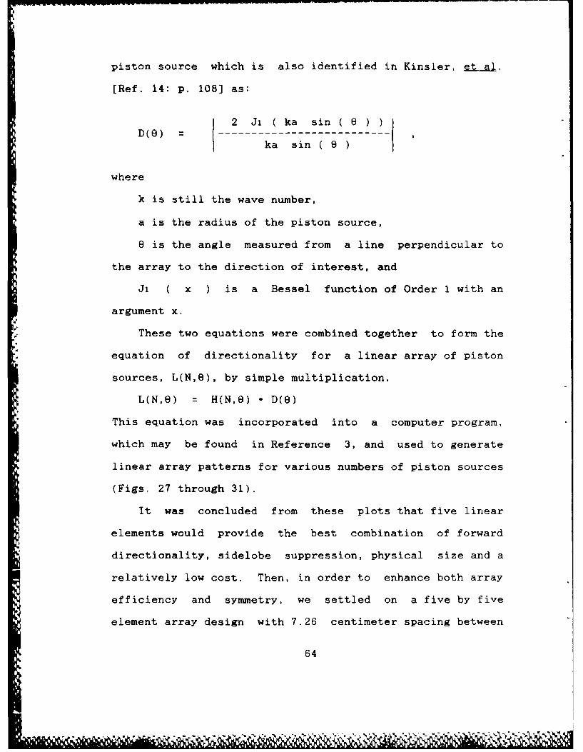
piston source which is also identified in Kinsler, et al.

(Ref. 14: p. 108] as:

2 Ji ( ka sin ( 8D(8)

ka sin ( 8

where

k is still the wave number,

a is the radius of the piston source,

8 is the angle measured from a line perpendicular to

the array to the direction of interest, and

Ji ( x ) is a Bessel function of Order 1 with an

argument x.

These two equations were combined together to form the

equation of directionality for a linear array of piston

sources, L(N,8), by simple multiplication.

L(N,e) = H(N,8) - D(8)

This equation was incorporated into a computer program,

which may be found in Reference 3, and used to generate

linear array patterns for various numbers of piston sources

(Figs. 27 through 31).

It was concluded from these plots that five linear

elements would provide the best combination of forward

directionality, sidelobe suppression, physical size and a

relatively low cost. Then, in order to enhance both array

efficiency and symmetry, we settled on a five by five

element array design with 7.26 centimeter spacing between

64

PATTERN OR 3 ELEMENTS PATTERN FOR 4 ELEMENTS

-10

- 10 -10U)

-JJ

-30 -3

Fig. 27. Three Element Array Fig. 28. Four Element Array

ATTERN FOR 5 ELEMENTS

-to

-3a

Fig. 29. Five Element Array

PATTERN FOR 5 ELEMENTS PATTERN FOR I ELEMENITS0

-10 -10

-30 -303

Fig. 30. Six Element Array Fig. 31. Seven Element Array

65

speakers in both the vertical and horizontal directions.

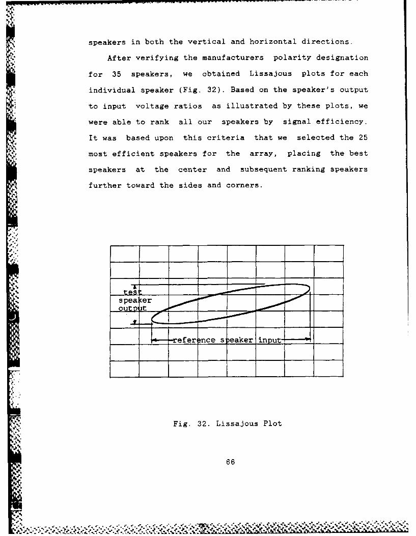
After verifying the manufacturers polarity designation

for 35 speakers, we obtained Lissajous plots for each

individual speaker (Fig. 32). Based on the speaker's output

to input voltage ratios as illustrated by these plots, we

were able to rank all our speakers by signal efficiency.

It was based upon this criteria that we selected the 25

most efficient speakers for the array, placing the best

speakers at the center and subsequent ranking speakers

further toward the sides and corners.

.p.

i ~speak:er 'outp..

-- refere.nee sp)eaker input----

Fig. 32. Lissajous Plot

66

. v,

3- . - W W--.-

The 25 selected speakers were --ounted in a five by five

planar array on a balsa wood insulated bilayered sheet

metal board. After wiring all the speakers in parallel, we

surrounded all the electrical connections and speaker backs

with two 3.0 centimeter layers of foam insulation

sandwiching a 1.0 millimeter lead sheet. Then the entire

array mounting was enclosed in a 44 by 44 by 5 centimeter

sheet metal box. This design was chosen to suppress

virtually all acoustic energy propagating out the rear

hemisphere of the array, while shielding the array from any

external electrical interference (Figs. 33 and 34).

67

W,SY ~ P" k k ..

I A........

Ul~

Fig.~4 33 Ara Pot

V ~68

P hA34

/

N

p4*

Fig. 34. Array PhotoRN,

69'.3

N, p

APPEDIX&

ENCLOSURE DESIGN

Acoustic echosounding has proven to be an extremely

useful technique for probing and analyzing the lower

atmosphere. In order to most efficiently utilize the

acoustic waves transmitted and later received by this

remote sensing method, it is essential to have an efficient

antenna with highly directive beams and strongly suppressed

sidelobes. Antenna design becomes increasingly more

important in a noisy environment where noise pollution

within the sidelobes may dominate the desired signal within

the main lobe. Hall and Wescott [Ref. 12] showed that

sidelobe suppression improved with higher frequencies.

Their studies showed that the measured 90 degree sidelobe

suppression ranged from 38 dB at 1 KHz to 50 dB at 5 KHz.

Furthermore, any significant improvement in sidelobe

suppression could only be obtained by surrounding the

antenna with an acoustic energy absorbing cuff or shroud.

In an effort to maximize our antenna main lobe to

sidelobe power ratio, we intend to operate only at high

frequencies as discussed in the previous section.

Additionally, we have designed an acoustic energy absorbing

enclosure. Many designs were considered based upon

70

previous research in the field of echosounding [Refs. 17

through 20]. In addition, we obtained the actual acoustic

beam patterns for our array using a computer program

written by LCDR Butler [Ref. 21] which we modified for our

purposes. This modified version of LCDR Butler's program

may be found in Reference 3. By rotating the array in an

anechoic chamber, we were able to produce highly accurate

polar plots of the array beam patterns (Figs. 35 and 36).

5 X 5 ACOUSTIC ARRAY BEAM PATTERN

IN.

R-.WM IEV-..26 rNU-50V FE-. H

/- /7N/

',

\ \ /

WJ

R-3.60 M MIKE VT= 8.2465 INPUT-50 V FRFQ=5. O KZ

, Fig. 35. Polar Plot of 5 X 5 Array Beam Pattern

71

I..

DIAGONAL 5 X 5 ACOUSTIC ARRAY BEAM PATTERN

/- r

4U MIKE

NN % %

-

-

R-3.80 M MIKE VT- 3.9497 INPUT-2.5 V FREQ-5.O KHZ

Fig. 36. Polar Plot of 5 X 5 Array Beam Patternat a 450 Aspect

72

These polar plots and the actual coordinates

corresponding to the individual data points confirmed the

computer prediction for the five element line array (Fig.

29). Additional polar plots obtained by varying both the

input array voltage and range between array and microphone

further support our claim that for a 5 KHz carrier

frequency, the main lobe is confined to a divergence angle

of 20 degrees. Since it is our aim to suppress all

sidelobes and utilize solely the main lobe, we chose not to

taper our enclosure as most previous researchers had.

Rather we designed the enclosure based upon the dimensions

of the array itself and the acoustic beams it generated.

Plywood was used for the construction of the enclosure

and provided not only a rigid, inexpensive framework, but

also proved to greatly attenuate external noise

interference. Anticipating all kinds of weather conditions

during data collection, the plywood enclosure was first

waterproofed with four coats of marine varnish. Grooved

joints, caulking and weather stripping were also design

considerations.

A millimeter layer of lead can suppress an acoustic

signal as much as 40 dB (Figs. 37 and 38). About 7.0

centimeters of corrugated, egg-carton design foam can

suppress a signal another 3 to 4 dB (Figs. 37 and 39).

Together they make an extremely efficient absorbing

material for use in our enclosure.

73

. .. .. ----. ..... - .-.- ., ..-- :v < ; : ' 4 ,*s.' ', ,K'< <

START Hz RAMGE: -19 dBYSV jj PAUSED

-19dIV

................................................. . . . . ........................................

/DIV I

. .... ........ ......... ......... .........

ST.mRT; 4 CJP3 HZ Bw: 1?.097 Hz STOP: 6 000 Hz

Fig. 37. Response Reference, No Insulation

START 4 008 Hz RAMGE -51 dIV STATUS: PAUSEDA:MfAG RMS:25

dV

.. .. .. .. ... . . . . . . . . . . . . . ... .. . . . . . . . . . . . . . . . ... ... . .

' Is .. . . . .. . . . .. . . . . . .

.3

/DIY

....... ........ ......... ......... ......... ......

" .

... .. ..1. .. . . . . . .. . . . . . . .. . . . ... ...

START: 4 00 Hz BW: 19.097 Hz STOP: 6 008 Hz-x: 508 Hz Y:-10.77 dBV

Fig. 38. Signal Suppression by Lead

74

'. *

START 4 088 Hz RANGE: -21 dBV STATUS: PAUSEDA:MAG RMS:25

-1'DIV, . .

. . . .

...... .....

• . . .............. . . ........... .. .

.. ...-... i .. . . .

-181 .f~

START: 4 008 Hz B;3 19.097 Hz STOP: 6 860 HzX: 5008 H: Yz-.22.78 dBV

Fig. 39. Signal Suppression by Foam

Lead-lined absorbing foam was glued to all inner

surfaces of the enclosure with two 1.0 millimeter layers of

lead overlapping at all corners. Strong aluminum brackets

were used to connect the four side panels to each other as

well as to the enclosure base (Figs. 40 through 42).

75

44m

I.-

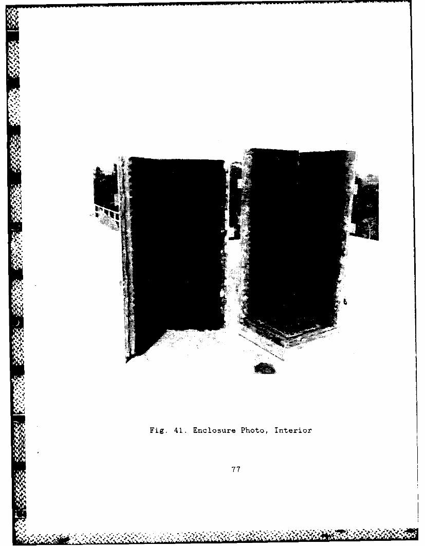
Fig. 41. Enclosure Photo, Interior

77

"MMg ."W'

9-m

Fi.4. nlsrePooBs it ra

I7

AmMDIX-D

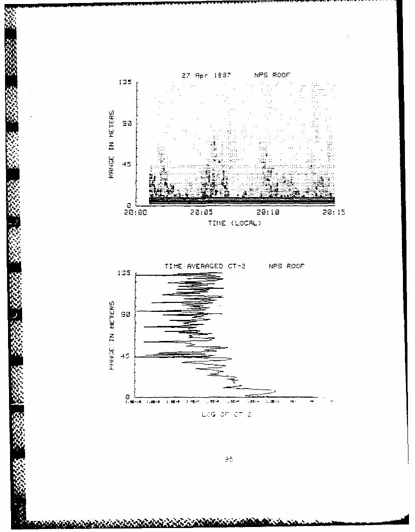
ECHOSOUNDER OUTPUT

Sixteen echosounder output traces were included to

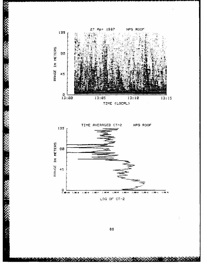
exhibit typical atmospheric activity. Many of the plots,

such as the 14:45, 15:30, and the 17:30 of 26 April and the

10:00, 11:15, 13:00, 14:15, 15:15, 16:15, and the 17:15 of

27 April, have convective plumes which are prevalent

whenever a heat flux between the surface and atmosphere

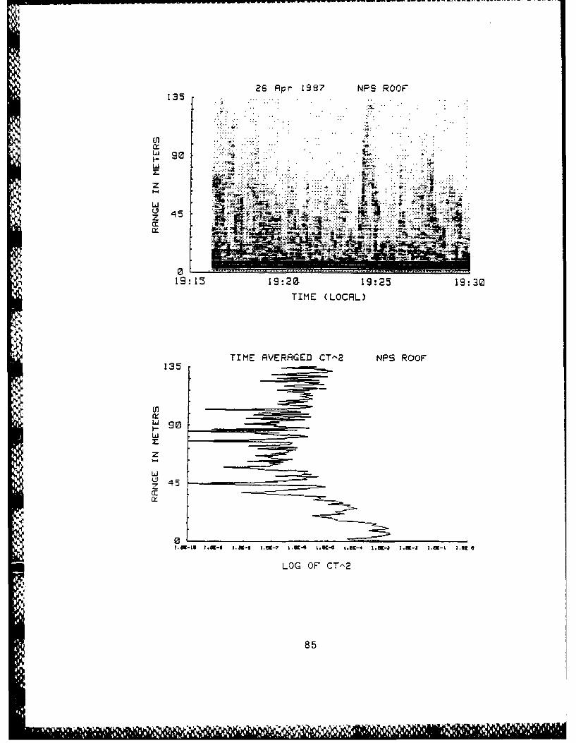
exists. The plots of 18:15 and 19:15 on the 26th of April

and of 18:00, 18:45 and 20:00 on the 27th of April clearly

show the passage of the neutral event which is encountered

when the atmospheric and surface temperature difference

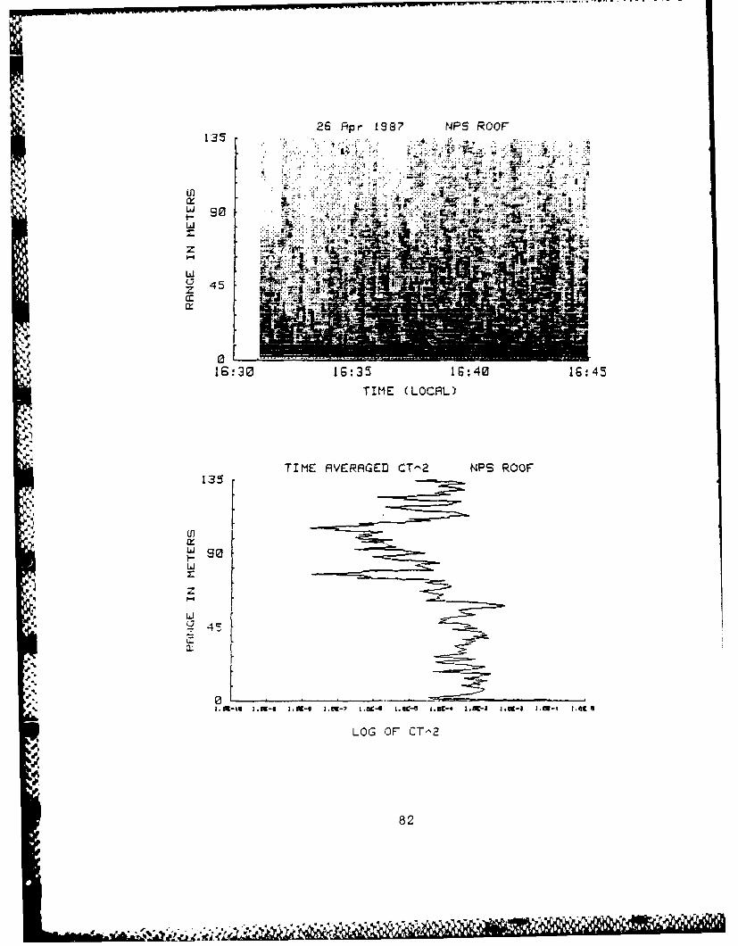
becomes negligible. Finally, the plot of 16:30 on 26 April

F. can be associated with strong winds which exhibit a

somewhat uniform return for all altitudes across the entire

15 minute interval of the trace.

The horizontal axis labels of the CT2 plots are small

and may be hard to read. This axis is a log scale

beginning with 1-10-10 at the left side of the plot and

ending with 1-100 at the right side of the plot. Each tick

mark moving left to right along this axis represents an

integer increase in the exponent of 10.

79

26 Apr 1987 NPS ROOF135

1-

LLL

14:45 14:50 1:515!00

TIME (LOCAL)

TIME AVERAGED CT-2 NPS ROOF135

= zz:

~90Ld

545

3.=-t@ J.5-4 1.5-4 2.-- i.VC-0 L.OC-0 t.K-4 J.W-i I.M-i L5O-L 3.5 IS

LOG OF CT-2

* 80

'SN'

26 Ppr 1387 NPS ROlOF

15t5

-pW

z -45

15 30 15 3 15401-4

~TM (LOCAL)~

- 5 '45

N- -g 3a- ). - ,'.M,-7 .J-g .'K-- IA- l- Ja- ,Kt LE1

TIMEO (LCAL)

1381

. .90 . . . .llm t ;t&

26 Apr 198? NPS ROOF135

LL '4 .....

045

.4,..

16.30 16 1:40 16: 45TIME (LOCSL)

TIME AVERAGED CT,1 NPS ROOF

1445

4'40

.4LO OF__ CT-

82

1526 Ppr 1987 NPS ROOF

Li

-44L6 -- f-Z ,..-,-

7-.:

- ,-

I4

017:30 17:35 17-40 17-45

TIME (LOCAL)

15- TIME AVERAGED CT-2 NPS ROOF

~ 0

1.2--

LOG OF C7^2

83

MEINw

26 Apr 198? NPS ROOF

.. .. ....

. ... .. .. ... .

so~ .. .... -.

454'

Q *0

TIME (LOCPL)

TIME AVERAGED CT^2 NPS F<CIOF135

~ 0

lu-U .U* .M-1 )A.-? t.6C-4 L.OC--l L.IC-4 I.K-1 I. - I.L i Ue

LOG OF CT'2

48

'SIf

26 Apr 1987 NPS ROF135. .

Li 41LU 90. .. .44

f.45~ ,

-+t 5w: *-s.

11S19:20 19.25 19:30TIME (LOCAL)

TIME AVERAGED CT^'2 NPS ROOF135

U

uz 45

-1y

85

27 Apr 1987 NPS ROOF135

... .. .

N ~4N

1 00 ....0. .... 10:1

103 0 10-05 1010 10:1

TIE(LCL

TIME AVRGDC-2 NSRO

S45L

LOG OF CT-2

86

2? Apr 1987 NPS ROOF135 .

Lii

LJS 9

44

TIME AVERAGED Cr-^ NPS ROOF135

z r

S45

0'2.in-6 ~.-O l -i ).m-7 t IC4* L.aC-3 t.aC-* 1.wj I.m-z ).(U-t ].Me '

LOG OF CT-h2

87

2' Api- 1987 NPS ROOF135

V ,. ~I:. Air.~90

b-4

LLI-- - *; WLl45

00

13 00 13:05 13 10 13.-15TIME (LOCAL)

TIME AVERRGED CT-'2 NPS ROOF135

S90

Li

454s

88

135 ~ 27 Apr 199? NPS ROOF

WP

Li~~v ... j~~4-L

fj..44

14-15 14:20 14:25 14:30

TIME (LOCAL)

135TIM1E AVERAG~ED CT-2 NPS ROOF

so

45-

LOG 0F C 7'2

89

2? Apr 193? NIPS ROOF

135.

s.o. .-...

453.

015- 15 15!20 15!25 15-3 0

4..TIME (LOCAL)

TIME AVERRGED CTh2 NIPS ROOF135

Ul

A4 32U I .M-1 J.-I -1 .~- L. C- L.OC-4 1.WE ~ -3 . -2. .-L l

LOG OF C7--2

90

- - C

37 Apr 199' NPS ROOF

1F 5 so 0M-'-,4,

-4 S..... n* 4c 4 '

16 i 16:20*~- !G 2 6 3

hi 91

27 Rpr 1099? NPS ROOF

. .. . .. . ....

TwA G ... . ..

CCC

017: 15 17:20 17 25 17-30

TIME (LOCAL)

TIME AVERAGED CTh2 NPS ROOF13 5

L

LOG OF- C7-2

92

S. . . L

27 Pp r 1998? N PS ROOF135

A-

z ....

.- A .. 4-

19:00 12:05 12: 10 12.-15

TIME (LOCAL)

TIME AVERA~GED CT'^2 NIPS ROOF135.

~ 93

Il------

11 Ppr 198? NPS ROOF

04-

z

194 48:5 1900

TIM (LCL

~~~TIME (L0CCE C^2NL RO

~so

F-

LAJ

49

2? Apr 1997 NPS ROOF135

Lfl

La

a ... . . . . . .. . . .. .. . .. . .

Zr ....... . .

C. ......

-- m. JA .

0 -

20:00 20:05 20:10 20:15

TIM E (LOCRL)

TIME MVERPv..Ef CT-. NPIS ROOF

-so,

La F

I -A184 972 DEVELOPMENT OF A DATA ANALYSIS SYSTEM FOR THE DETECTION 2/2OF LOWER LEVEL AT (U) NAVAL POSTGRADUATE SCHOOL

17 SI FE MONTEREY CA M R N ROBLENSKI JUN 87 FG41 N

*"1 111.2*

L3 6

U . -

IIIJIIL252

MICROCOPY RESOLUTION TEST CHART

NATInNAL BUREAL, Of SANDARD , 1963 A

;l

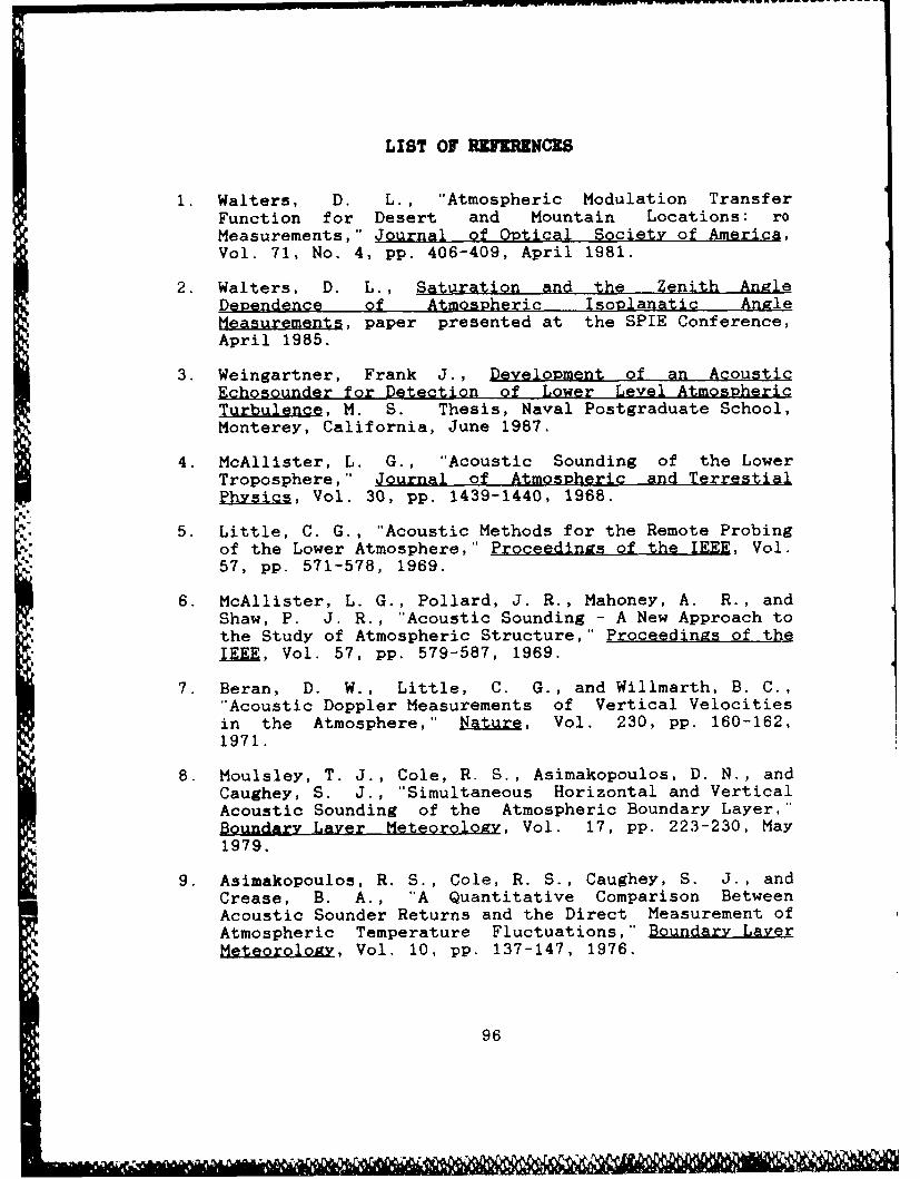
LIST Of RUFaMNCES

1. Walters, D. L., "Atmospheric Modulation TransferFunction for Desert and Mountain Locations: roMeasurements," Journal of Optical Society of America,Vol. 71, No. 4, pp. 406-409, April 1981.

2. Walters, D. L., Saturation and the Zenith AnoleDependence of Atmospheric Isoplanatic AngleMeasurements, paper presented at the SPIE Conference,April 1985.

3. Weingartner, Frank J., Development of an AcousticEchosounder for Detection of Lower Level AtmosphericTurbulen, M. S. Thesis, Naval Postgraduate School,Monterey, California, June 1987.

4. McAllister, L. G., "Acoustic Sounding of the LowerTroposphere," Journal of Atmospheric and TerrestialPhysics, Vol. 30, pp. 1439-1440, 1968.

5. Little, C. G., "Acoustic Methods for the Remote Probingof the Lower Atmosphere," Proceedings of the IEEE, Vol.57, pp. 571-578, 1969.

6. McAllister, L. G., Pollard, J. R., Mahoney, A. R., andShaw, P. J. R., "Acoustic Sounding - A New Approach tothe Study of Atmospheric Structure," Proceedings of theIEEE, Vol. 57, pp. 579-587, 1969.

7. Beran, D. W., Little, C. G., and Willmarth, B. C.,"Acoustic Doppler Measurements of Vertical Velocitiesin the Atmosphere," Nature, Vol. 230, pp. 160-162,1971.

8. Moulsley, T. J., Cole, R. S., Asimakopoulos, D. N., andCaughey, S. J., "Simultaneous Horizontal and VerticalAcoustic Sounding of the Atmospheric Boundary Layer,"Boundary Layer Meteoroloay, Vol. 17, pp. 223-230, May1979.

9. Asimakopoulos, R. S., Cole, R. S., Caughey, S. J., andCrease, B. A., "A Quantitative Comparison BetweenAcoustic Sounder Returns and the Direct Measurement ofAtmospheric Temperature Fluctuations," Boundary LayerMgtor.ology, Vol. 10, pp. 137-147, 1976.

96

6 - h~f6L~ .........

10. Neff, W. D., "Quantitative Evaluation of AcousticEchoes from the Planetary Boundary Layer," NOAATechnical Report ERL 322-WPL 38, June 1975.

11. Tatarski, V. I., The Effects of the TurbulentAtmosphere on Wave Propaaation, U. S. Department ofCommerce, Washington, D. C., 1971; available fromNational Technical Information Service, Springfield,VA. 22161.

12. Hall Jr., F. F., and Wescott, J. W., "Acoustic Antennasfor Atmospheric Echo Sounding," Journal of theAcoustical Society of America, Vol. 58, No. 5, pp.1376-1382, November 1974.

13. Walters, Donald L., Naval Postgraduate School,Monterey, California. Personal Communication, 7January 1987.

14. Kinsler, L. E., Frey, A. R., Coppens, A. B., andSanders, J. V., Fundamentals of Acoustics, John Wileyand Sons, New York, 1982.

15. Fuller, Robert J., Parametric Analysis of EchosounderPerformance, M. S. Thesis, Naval Postgraduate School.Monterey, California, September 1985.

16. Motorola Piezo Ceramic Speakers Catalog, Motorola Inc.,Communications Systems Divisions, p. R29-5-1B, 1978.

17. Strand, 0. N., "Numerical Study of the Gain Pattern ofa Shielded Acoustic Antenna," Journal of the AcousticalSociety of America, Vol. 49, No. 6 (Part 1), pp. 1698-1703, June 1971.

18. Adekola, S. A., "Toward a More General IntegralFormulation of the Pressure Field of an EchosondeAperture Antenna," Journal of the Acoustical Society ofAmerica, Vol. 60, No. 1, pp. 230-239, July 1976.

19. Adekola, S. A., "Concerning the Influence of EchoCarrier Frequencies and Antenna Dimensions on thePerformance of Echosonde (Acoustic-Radar) Antennas,"Journal of the Acoustical Society of America, Vol. 62,No. 3, pp. 524-542, September 1977.

20. Adekola, S. A., and Davis, D. T., "The Effects ofPhase-front Distributions on Echosonde AntennaRadiation Patterns," R4dio Science, Vol. 12, pp. 11-22,January - February 1977.

97

21. Butler, John D., Development, Validation and Use of aComputer-Controlled System for the Investigation ofPhase and Amplitude Shaded Acoustic Arrays, M. S.Thesis, Naval Postgraduate School, Monterey,California, December 1986.

98

INITIAL DISTRIBUTION LIST

No. of Copies

1. Defense Technical Information Center 2Cameron StationAlexandria, VA 22304-6145

2. Library, Code 0142 2Naval Postgraduate SchoolMonterey, CA 93943-5002

3. Prof. Donald L. Walters 5Department of Physics (Code 61We)Naval Postgraduate SchoolMonterey, CA 93943-5004

4. Prof. Steven L. GarrettDepartment of Physics (Code 61Gt)Naval Postgraduate SchoolMonterey, CA 93943-5004

5. Commandant (G-PTE) 2U. S. Coast Guard2100 2nd Street, S.W.Washington, D. C. 20593

6. Commanding Officer 3U. S. Coast Guard Research and Development CenterAvery PointGroton, CT 06340-6096ATTN: LT. M. WROBLEWSKI

7. Prof. Karlheinz E. WoehlerChairman, Department of Physics (Code 61Wh)Naval Postgraduate SchoolMonterey, CA 93943-5004

99

ps~.