1

A Decoupled Approach for Near-Field Source Localization Using a Single Acoustic Vector Sensor

(The final publication is available at www.springerlink.com

DOI : 10.1007/s00034-012-9508-9)

V. N. Hari, A. B. Premkumar, X. Zhong

School of Computer Engineering, Nanyang Technological University, Singapore 639798,

harivishnu@gmail.com

Abstract

This paper considers the problem of three-dimensional (3-D, azimuth, elevation and range)

localization of a single source in the near-field using a single acoustic vector sensor (AVS). The

existing multiple signal classification (MUSIC) or maximum likelihood estimation (MLE)

methods which require a 3-D search over the location parameter space are computationally very

expensive. A computationally simple method previously developed in [33], which we refer to as

Eigen-value decomposition and Received Signal strength Indicator based method (Eigen-RSSI),

was able to estimate 3-D location parameters of a single source efficiently. However, it can only

be applied to an extended AVS which consists of a pressure sensor separated from the velocity

sensors by a certain distance. In this paper, we propose a uni-AVS MUSIC (U-MUSIC) approach

for 3-D location parameter estimation based on a compact AVS structure. We decouple the 3-D

localization problem into step by step estimation of azimuth, elevation and range, and derive

closed form solutions for these parameter estimates by which a complex 3-D search for the

parameters can be avoided. We show that the proposed approach outperforms the existing Eigen-

RSSI method when the sensor system is required to be mounted in a confined space.

Keywords: Acoustic Vector Sensor, Localization, near-field, MUSIC, DOA estimation

1. Introduction

An acoustic vector sensor (AVS) is capable of measuring particle velocities as well as acoustic

pressure at a point in space, and can estimate the direction of arrival (DOA) of a source

unambiguously [8, 17, 33]. Both theoretical studies and experimental setups such as the DIFAR

(DIrectional Frequency Analysis and Recording) array [3] and the recently conducted Makai

experiment [18] have shown that an AVS is superior to the traditional acoustic pressure sensor in

DOA estimation. In the recent past, array signal processing approaches such as the Capon

beamformer [8], multiple signal classification (MUSIC) [31, 39], estimation of signal parameters

via rotational invariance (ESPRIT) [25, 27–29], Root- MUSIC [30] and other approaches [2, 10,

11, 16, 35] have been employed for AVS signal based DOA estimation. The impressive

performance of the vector sensors has also been demonstrated in numerous other signal processing

problems such as source tracking [5, 36–38], detection [6, 7, 38], communication [1, 21, 22] and

inversion problems [19, 20].

This paper focuses on the problem of near-field localization of a source. Near-field localization

has a broad range of applications such as sonar [13], seismic exploration [24] and electronic

surveillance [14], and recent research has attempted to elevate the performance of near-field

localization using the advantages of an AVS. Tichavsky et al [25] developed a uni-vector-

hydrophone based ESPRIT method using a single vector hydrophone for two-dimensional azimuth

and elevation angle estimation, for sources in the near-field. Xu et al [34] presented an analysis of

a conjugate multiple-invariance ESPRIT method, which can be used for direction-finding of non-

circular signals using a single AVS.

Recently, Wu, Wong and Lau [32] presented the array manifold of an AVS, with co-located

pressure and velocity sensors, for a point source located in the near-field. AVS are generally

2

constructed with such a compact geometry, in the sense that they contain co-located pressure and

velocity sensors [17]. The DIFAR array [3], Swallow floats [4] and the Wilcoxon array [18],

which have all been deployed successfully, are examples of the usage of such a compact AVS. The

pressure measurement in the measurement manifold of a compact AVS is dependent on the range

of the source from the sensor, when the source is located in the near-field [32]. Since the manifold

is a function of range in the near-field scenario, a single compact AVS can be used to estimate the

range in addition to the source azimuth and elevation. Since the spherical coordinates of a source

are specified by the range, elevation and azimuth, a single compact AVS is capable of performing

3-D source localization. However, using asymptotically efficient methods such as MLE or MUSIC

for this involves a computationally expensive search for the location parameters in the azimuth-

elevation- range space [23].

Wu and Wong [33] presented an approach in which this complex 3D search for the source

location parameters is avoided. Their method employs a ‘spatially extended’ AVS, which is

constructed by using a co-located triad of velocity sensors and a pressure sensor placed at a certain

distance away from the triad. Initially, the azimuth and elevation of the signal source are estimated

from the velocity sensor data first using an eigen-structure method. The range is then estimated by

using the Received Signal Strength Indication (RSSI) approach. This combination of eigen-

structure based DOA estimation and RSSI based range estimation, which will be referred to as the

Eigen-RSSI method in the rest of the paper, has been employed for 3-D source localization in [33].

Even though the Eigen-RSSI method performs impressively in localization of sources using an

extended sensor system consisting of two separated ‘anchor nodes’ (the pressure sensor and the

velocity sensor triad), it faces a limitation in its requirement for the pressure sensor to be located at

a specific distance and direction from the velocity sensors. Thus the extended sensor system loses

out on a significant advantage in using a single AVS for localization, namely, the compactness.

Lack of compactness is a severe limitation in situations that require the sensor system to be

accommodated in a restricted space for localization, such as autonomous underwater vehicles,

room object tracking, and hearing aid systems. The sensor arrangement for the Eigen-RSSI method

also requires additional calibration of the separated sensor system, and this constitutes additional

complexity in its deployment.

In this paper, we present a novel approach for 3-D localization of the source using a single

compact AVS based on the near-field array manifold presented in [32], which overcomes

disadvantages of the above mentioned approaches. It employs the signal eigen-vector of the data

correlation matrix similar to MUSIC [23], and yields closed form solutions for the estimation of

location parameters. The method, which will be referred to as uni-AVS MUSIC (U-MUSIC),

decouples the 3-D localization problem into step-by-step estimation of the location parameters and

does not require a complex search for the location parameters as conventional MUSIC does. The

decoupling of range-estimation from DOA estimation is not new in itself. Some methods proposed

previously in the literature, such as those by Weiss and Friedlander [26] and Hung et al [12], have

proven useful in reducing the complexity of MUSIC-based source localization using an array of

pressure sensors. Weiss and Friedlander reduced the complexity of a two-dimensional range-

bearing search by converting it into a one-dimensional search for range, combined with

polynomial rooting procedure that replaces the azimuth search. Hung et al further extended this to

3-D source localization by reducing the 3-D search to a range search, combined with polynomial

rooting for azimuth and elevation. While these methods dealt with measurements obtained from

arrays of acoustic pressure sensors, our method concerns the decoupling of range, azimuth and

elevation estimates from the measurements obtained from a single AVS. Note that U-MUSIC is

also not be confused with Root-MUSIC [29] since the former does not require an array of AVS.

The main advantage of U-MUSIC is that it avoids the need for a 3-D search in the azimuth-

elevation-range space and hence reduces the computational complexity. We will show that U-

MUSIC yields asymptotically efficient performance. Furthermore, this method can be applied in a

compact AVS system.

The outline of this paper is as follows. In Section 2, we present the measurement model for the

localization problem. Section 3 gives a brief description of the Eigen-RSSI source localization

algorithm, and describes the novel U-MUSIC algorithm of near-field source localization using a

single compact AVS. Section 4 presents a simple measure for the comparison of the performance

of the range estimation obtained using extended and compact AVS. Section 5 presents results

3

depicting the performance of the U-MUSIC algorithm and its comparison with some of the

existing methods, and Section 6 concludes the paper.

2. Measurement model of localization

Assume that a single narrowband acoustic signal source is present in an isotropic homogeneous

medium. The wave-fronts of the waves emanating from the source can thus be considered to be

either spherical for a receiver in the near-field or planar when the receiver is in the far-field. The

far-field scenario refers to the cases where krs >>1 [32], where rs is the range of the source from

the sensor and k is the wavenumber defined as k = 2π/λ (λ is the wavelength of the source signal).

Let y(t) be the tth

snapshot of the 4 1 measurement vector at the output of the AVS. The complex

measurement vector for a general case (far-field or near-field) can be written as [32]

y(t) = a s(t) + e(t) (1)

where s(t) refers to the tth

snapshot of the source signal, a refers to the 4 1 manifold of the AVS,

and e(t) denotes a 4 1 vector of the additive zero-mean white environmental noise in the

measurement of the tth

snapshot. The noise vector has a covariance matrix C0. With N measured

snapshots, the collected 4N 1 data set is represented as

Y = [y(1)T … y(N)

T]

T = s a + E (2)

where s = [s(1)… s(N)]T denotes the signal vector and E=[e(1)

T … e(N)

T]

T represents a 4N 1

environmental noise vector with a spatio-temporal covariance matrix C = IN C0, where IN

represents the N N identity matrix, denotes the kronecker product, and superscript T denotes

the matrix transpose, respectively. We assume that the velocity components are scaled by the

factor ρc, and this is generally assumed to be known (ρ is the ambient density and c is the speed of

propagation of the acoustic wave in the medium).

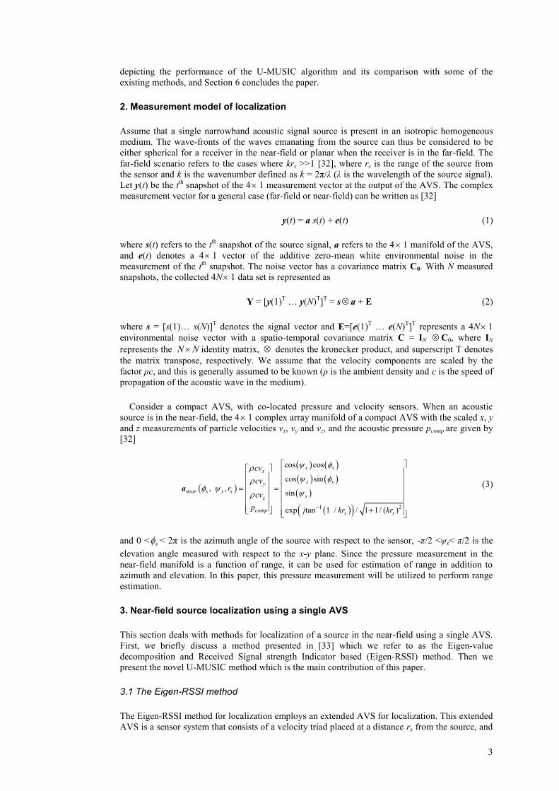
Consider a compact AVS, with co-located pressure and velocity sensors. When an acoustic

source is in the near-field, the 4 1 complex array manifold of a compact AVS with the scaled x, y

and z measurements of particle velocities vx, vy and vz, and the acoustic pressure pcomp are given by

[32]

1 2

cos cos

 cos sin , ,

 sin 

   exp tan 1 / / 1 1/ ( )

s sx

s sy

near s s ssz

comps s

cv

cvr

cv

p j kr kr

a

(3)

and 0 < s < 2π is the azimuth angle of the source with respect to the sensor, -π/2 <ψs< π/2 is the

elevation angle measured with respect to the x-y plane. Since the pressure measurement in the

near-field manifold is a function of range, it can be used for estimation of range in addition to

azimuth and elevation. In this paper, this pressure measurement will be utilized to perform range

estimation.

3. Near-field source localization using a single AVS

This section deals with methods for localization of a source in the near-field using a single AVS.

First, we briefly discuss a method presented in [33] which we refer to as the Eigen-value

decomposition and Received Signal strength Indicator based (Eigen-RSSI) method. Then we

present the novel U-MUSIC method which is the main contribution of this paper.

3.1 The Eigen-RSSI method

The Eigen-RSSI method for localization employs an extended AVS for localization. This extended

AVS is a sensor system that consists of a velocity triad placed at a distance rs from the source, and

4

a pressure sensor separated by a distance d from the velocity sensors in a known direction. Eigen-

RSSI [33] initially estimates azimuth and elevation using elements of the eigen-vector obtained

from eigen-decomposition of the data. It then uses the RSSI method to estimate the range of the

source, which is described below.

The magnitude of the pressure field pcomp at the location of the velocity sensors is estimated

from the particle velocity measurements using the relation 1

22 2 comp x y zp c v v v (4)

The magnitude of the ratio of this estimated pressure field with the pressure field pext measured at

the extended pressure sensor is known to be equal to

|pcomp/pext| = (rext/rs), (5)

where rext is the range of the extended pressure sensor from the source. This relation assumes that

the acoustic energy path loss model of the signal follows the inverse square law [33]. 2

The

extension d of the pressure sensor from the velocity sensors is known. The direction of this

extension is also known. For example, in the case when the extension d is assumed to be along the

x axis (as assumed in [33]), we have the relation

2 2 22 cos( )cos( ) sin( )cos( ) sin( ) ext s s s s s s s sr r d r r (6)

The relation in (6) can be easily obtained from vector resolution of rs along the x, y and z

directions. In (6), the cases ‘-d’ and ‘+d’ refer to the two cases when the pressure sensor is closer

to and further away from the source than the velocity sensors, respectively. From (4), (5) and (6),

the value of rs is determined. This constitutes the RSSI method of range estimation.

The estimation of range using RSSI, in addition to the estimation of the azimuth and elevation,

comprises complete localization of the source.

3.2 The uni-AVS MUSIC method

In this subsection, we elaborate on a novel method that is derived from MUSIC, for near-field

source localization using a compact AVS. MUSIC is an efficient method that has been shown to

be asymptotically equivalent to the MLE [23]. It does not require the assumption that the

environmental noise is Gaussian in nature [23] and is hence effective in finite-variance non-

Gaussian environmental noise also. This makes MUSIC useful in several applications such as

underwater acoustics, since the acoustic noise in the ocean is often non-Gaussian in character [15].

Our objective here is to obviate the need for the complex 3-D search involved in MUSIC-based

localization with an AVS.

At the outset, recall that conventional MUSIC [24] requires a computationally intensive 3D

search for the largest peak in the beamforming spectrum to find the estimates , and r of the

azimuth, elevation and range, respectively. For the localization of a single source, MUSIC

searches for the highest peak of the MUSIC spectrum given by

AMUSIC(ω) = aH(ω)uu

H a(ω), (7)

where ω represents the vector of parameters being estimated, a represents a steering vector that is

a function of ω, and u = [u1 .. u4]T represents the 4x1 signal eigen-vector obtained from the eigen-

value decomposition of the data correlation matrix, corresponding to the largest eigen-value.

MUSIC searches for the steering vector that is best contained in the signal subspace spanned by u.

1 This approximation discards the term 21/ 1 1/ ( )skr .

2 The Eigen-RSSI method allows incorporation of path loss models other than the inverse square law also.

5

The signal eigen-vector u has the same form as that of the array manifold a, and can be

represented by [33]

je

au

a, (8)

where ||.|| stands for the Frobenius norm and η symbolizes an unknown phase. The normalization

term ||a|| has been introduced into the denominator because by definition of an eigen-vector, ||u|| =

1. The above approximation converges to equality under noiseless or asymptotic conditions.

We will now describe the uni-AVS MUSIC algorithm. The aim is to obtain closed form

expressions for the estimates of the azimuth, elevation and range. These expressions, which are

derived from MUSIC, eliminate the need for a complex 3-D search in the MUSIC spectrum as

required by conventional MUSIC. This is achieved using a twofold approach. Firstly, the problem

of simultaneously estimating all three source location parameters is broken down into individual

1D MUSIC searches by using elements of the signal eigen-vector u. Then, the closed form

expressions for the estimates of the location parameters are obtained by maximizing the MUSIC

spectrums associated with each 1D search. The algorithm first obtains the azimuth estimate by

decoupling it from the overall 3D search, which is facilitated by restricting the measurements used

to the two horizontal velocity measurements. Secondly, it estimates the elevation, which can now

be estimated using the three velocity sensor measurements and the previously obtained azimuth

estimate. The range is estimated in the final step using measurements from all four channels, as it

requires use of the DOA estimates.

From the expression for the near-fold manifold in (3), and from (8), we observe that the

truncated signal eigen-vector u , that contains elements of u corresponding to the horizontal (x

and y) velocities alone, can be expressed as a function of the source azimuth angle s as

1 2 1 ( ) T

su u u c a , (9)

where

cos , sinT

a , (10)

and c1 ≈ ejη

cos(ψ)/||a|| is an unknown constant. The estimate of the azimuth angle may be found

by searching for the angle that maximizes the projection of the steering vector a into the

signal subspace spanned by the vector u . This allows a decoupled search for the estimate of the

azimuth alone, and can be expressed as

21 2

ˆ arg max [ ]   arg max [| cos   sin | ],  H H u u a u u a (11)

where |.| denotes the absolute value. The estimate can be obtained by maximization of the term

within brackets in (11), by setting its derivative with respect to to zero, which yields the

quadratic equation:

Re(u1*u2) tan

2( ) + (|u1|

2 - |u2|

2) tan( ) - Re(u1

*u2) = 0, (12)

where x* and Re(x) refer to the conjugate and real part of x, respectively. Solving (12) yields the

closed form estimate for the azimuth as:

= tan-1

(l + 2 1l ), (13)

6

where

l = 0.5 (|u2|2 - |u1|

2)/ Re(u1

*u2). (14)

Note that the tan-1

(.) function in (13) can yield two possible values for , which are separated by

an angle of π. In other words, if is an estimate of the azimuth, then ( + π) is also a possible

estimate. This is an ambiguity that is inherent in DOA estimation using velocity sensors alone

[25]. The ambiguity can be resolved using the pressure measurement also, as will be explained at

the end of this section. For now, we will continue with our algorithm by selecting the value of

that lies within the interval [0, π], and we will resolve the direction ambiguity in the final step.

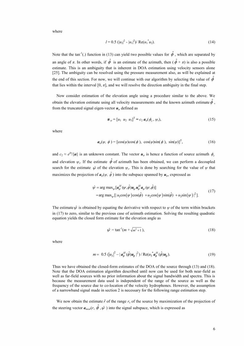
Now consider estimation of the elevation angle using a procedure similar to the above. We

obtain the elevation estimate using all velocity measurements and the known azimuth estimate ,

from the truncated signal eigen-vector uψ defined as

u ψ = [u1 u2 u3]T = c2 aψ( s , ψs), (15)

where

aψ(ψ, ) = [cos(ψ)cos( ), cos(ψ)sin( ), sin(ψ)]T, (16)

and c2 ≈ ejη

/||a|| is an unknown constant. The vector uψ is hence a function of source azimuth s

and elevation ψs. If the estimate of azimuth has been obtained, we can perform a decoupled

search for the estimate of the elevation ψs. This is done by searching for the value of ψ that

maximizes the projection of aψ(ψ, ) into the subspace spanned by uψ, expressed as

21 2 3

ˆ ˆˆ arg max [ ( , ) ( , )]

ˆ ˆ  arg max [| cos cos( )   cos sin( ) sin | ]. 

H H

u u u

a u u a (17)

The estimate is obtained by equating the derivative with respect to ψ of the term within brackets

in (17) to zero, similar to the previous case of azimuth estimation. Solving the resulting quadratic

equation yields the closed form estimate for the elevation angle as

= tan-1

(m + 2 1m ), (18)

where

2 2 *3 3

ˆ ˆ 0.5 ( | ( ) | ) / Re( ( ) ). H Hm u u a u a u (19)

Thus we have obtained the closed-form estimates of the DOA of the source through (13) and (18).

Note that the DOA estimation algorithm described until now can be used for both near-field as

well as far-field sources with no prior information about the signal bandwidth and spectra. This is

because the measurement data used is independent of the range of the source as well as the

frequency of the source due to co-location of the velocity hydrophones. However, the assumption

of a narrowband signal made in section 2 is necessary for the following range estimation step.

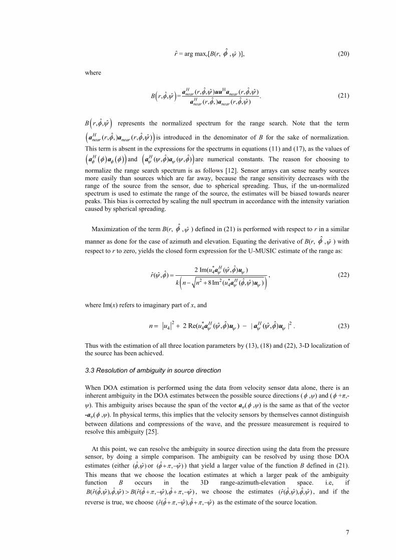
We now obtain the estimate r of the range rs of the source by maximization of the projection of

the steering vector anear(r, , ) into the signal subspace, which is expressed as

7

r = arg maxr[B(r, , )], (20)

where

Hˆ ˆˆ ˆ( , , ) ( , , )ˆ ˆ, , = .

ˆ ˆ ˆ( , , ) ( , , )

Hnear near

Hnear near

r rB r

r r

a uu a

a a (21)

B ˆ ˆ, ,r represents the normalized spectrum for the range search. Note that the term

ˆ ˆ ˆ( , , ) ( , , )Hnear nearr r a a is introduced in the denominator of B for the sake of normalization.

This term is absent in the expressions for the spectrums in equations (11) and (17), as the values of

H a a and ˆ ˆ( , ) ( , )H

a a are numerical constants. The reason for choosing to

normalize the range search spectrum is as follows [12]. Sensor arrays can sense nearby sources

more easily than sources which are far away, because the range sensitivity decreases with the

range of the source from the sensor, due to spherical spreading. Thus, if the un-normalized

spectrum is used to estimate the range of the source, the estimates will be biased towards nearer

peaks. This bias is corrected by scaling the null spectrum in accordance with the intensity variation

caused by spherical spreading.

Maximization of the term B(r, , ) defined in (21) is performed with respect to r in a similar

manner as done for the case of azimuth and elevation. Equating the derivative of B(r, , ) with

respect to r to zero, yields the closed form expression for the U-MUSIC estimate of the range as:

*4

2 2 *4

ˆˆ2 Im( ( , ) )ˆˆˆ( , )

ˆ ˆ8Im ( ( , ) )

H

H

ur

k n n u

a u

a u

, (22)

where Im(x) refers to imaginary part of x, and

2 * 24 4

ˆ ˆˆ ˆ 2 Re( ( , ) ) | ( , ) | H Hn u u a u a u . (23)

Thus with the estimation of all three location parameters by (13), (18) and (22), 3-D localization of

the source has been achieved.

3.3 Resolution of ambiguity in source direction

When DOA estimation is performed using the data from velocity sensor data alone, there is an

inherent ambiguity in the DOA estimates between the possible source directions ( ,ψ) and ( +π,-

ψ). This ambiguity arises because the span of the vector aψ( ,ψ) is the same as that of the vector

-aψ( ,ψ). In physical terms, this implies that the velocity sensors by themselves cannot distinguish

between dilations and compressions of the wave, and the pressure measurement is required to

resolve this ambiguity [25].

At this point, we can resolve the ambiguity in source direction using the data from the pressure

sensor, by doing a simple comparison. The ambiguity can be resolved by using those DOA

estimates (either ˆ ˆ( , ) or ˆ ˆ( , ) ) that yield a larger value of the function B defined in (21).

This means that we choose the location estimates at which a larger peak of the ambiguity

function B occurs in the 3D range-azimuth-elevation space. i.e, if ˆ ˆ ˆ ˆˆ ˆ ˆ ˆˆ ˆ( ( , ), , ) ( ( , ), , ) B r B r , we choose the estimates ˆ ˆˆ ˆˆ( ( , ), , )r , and if the

reverse is true, we choose ˆ ˆˆ ˆˆ( ( , ), , ) r as the estimate of the source location.

8

Alternatively, we may also limit the search interval of the azimuth to [0, π] as mentioned in

[25], and this leads to no ambiguity in DOA. Also, if any prior information is available on the

location of the source, such as whether it is located within the upper (ψ>0) or lower (ψ<0)

hemisphere, or whether it is located in the left ( 0, ) or right ( ,2 ) hemisphere, this

information is enough to resolve the ambiguity, and one does not have to resort to the

disambiguation method described in this section.

4. A performance measure for comparison

We propose a simple measure to theoretically compare the accuracy of range estimation using the

Eigen-RSSI and U-MUSIC methods, which is the sensitivity of their range estimation methods to

the range rs. This range-sensitivity provides a measure of performance of range-estimation which

is simpler to compute, thus alleviating the need to do time-consuming Monte-Carlo simulations to

compare the methods.

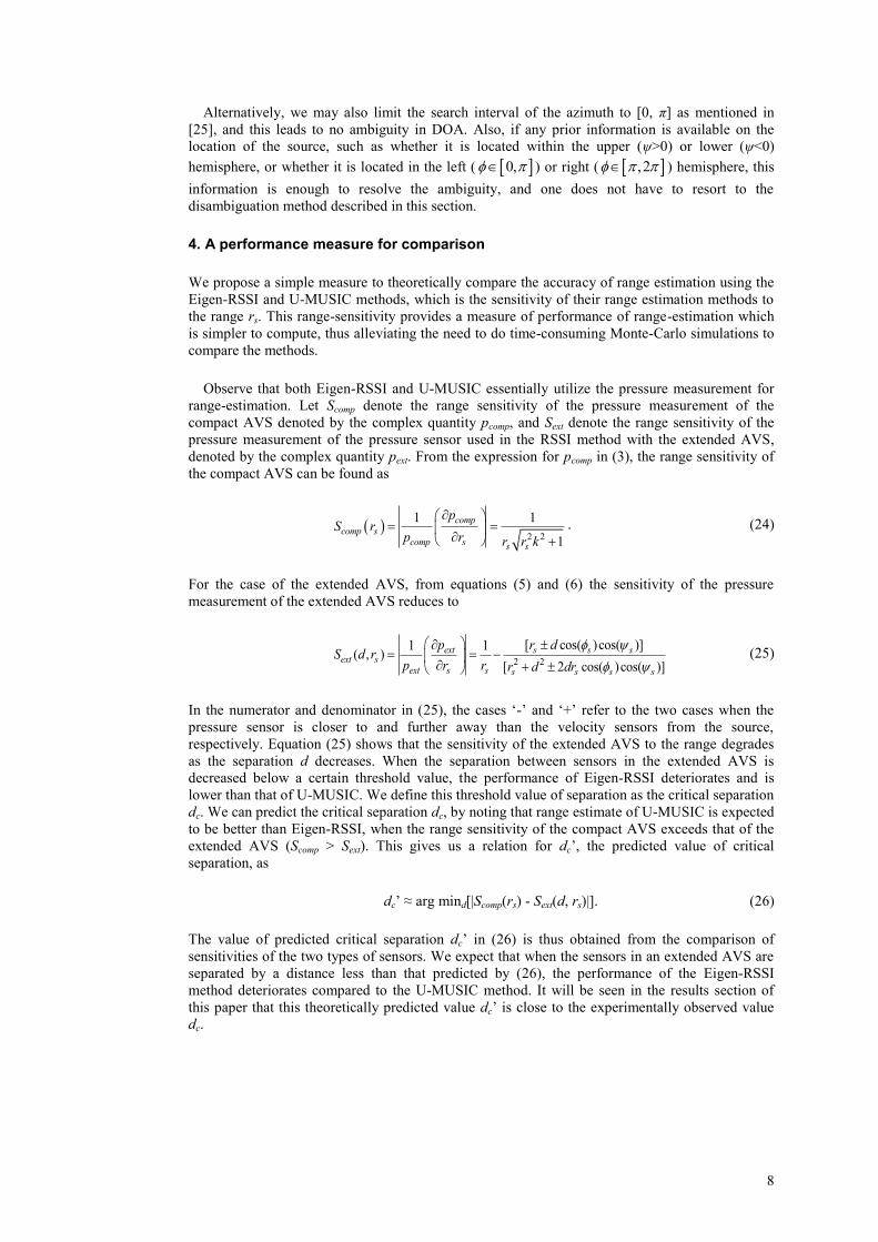
Observe that both Eigen-RSSI and U-MUSIC essentially utilize the pressure measurement for

range-estimation. Let Scomp denote the range sensitivity of the pressure measurement of the

compact AVS denoted by the complex quantity pcomp, and Sext denote the range sensitivity of the

pressure measurement of the pressure sensor used in the RSSI method with the extended AVS,

denoted by the complex quantity pext. From the expression for pcomp in (3), the range sensitivity of

the compact AVS can be found as

2 2

1 1

1

comp

comp scomp s s s

pS r

p r r r k

. (24)

For the case of the extended AVS, from equations (5) and (6) the sensitivity of the pressure

measurement of the extended AVS reduces to

2 2

[ cos( )cos( )]1 1( , )

[ 2 cos( )cos( )]

ext s s sext s

ext s s s s s s

p r dS d r

p r r r d dr

(25)

In the numerator and denominator in (25), the cases ‘-’ and ‘+’ refer to the two cases when the

pressure sensor is closer to and further away than the velocity sensors from the source,

respectively. Equation (25) shows that the sensitivity of the extended AVS to the range degrades

as the separation d decreases. When the separation between sensors in the extended AVS is

decreased below a certain threshold value, the performance of Eigen-RSSI deteriorates and is

lower than that of U-MUSIC. We define this threshold value of separation as the critical separation

dc. We can predict the critical separation dc, by noting that range estimate of U-MUSIC is expected

to be better than Eigen-RSSI, when the range sensitivity of the compact AVS exceeds that of the

extended AVS (Scomp > Sext). This gives us a relation for dc’, the predicted value of critical

separation, as

dc’ ≈ arg mind[|Scomp(rs) - Sext(d, rs)|]. (26)

The value of predicted critical separation dc’ in (26) is thus obtained from the comparison of

sensitivities of the two types of sensors. We expect that when the sensors in an extended AVS are

separated by a distance less than that predicted by (26), the performance of the Eigen-RSSI

method deteriorates compared to the U-MUSIC method. It will be seen in the results section of

this paper that this theoretically predicted value dc’ is close to the experimentally observed value

dc.

9

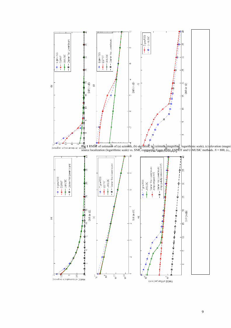
Fig 1 RMSE of estimates of (a) azimuth, (b) elevation, (c) azimuth (magnified, logarithmic scale), (c) elevation (magnified, logarithmic scale), (e) range (logarithmic scale), and (f) RLEE of

source localization (logarithmic scale) vs. SNR, comparing Eigen-RSSI, ESPRIT and U-MUSIC methods. N = 800, (xs, ys, zs) = (63.3, 75.4, 17.4) m.

10

5. Simulation Results

This section presents results to demonstrate the performance of the U-MUSIC method. Recall that

U-MUSIC uses the compact AVS to estimate the azimuth, elevation and range. In contrast, Eigen-

RSSI [33] employs an extended AVS, in which the pressure sensor is separated from the velocity

sensors in the x direction (as used in [33]) by a known distance d. The noise (in each snapshot) at

the AVS is assumed to be Gaussian in nature and have the internal covariance matrix C0 given by

[9]

320

/ 3

1p T

IC

0

0, (27)

where 0 is a 3x1 vector of zeros. This model assumes that the noise at all measurement channels is

uncorrelated, spherically isotropic, and the variance 2p of the noise of the pressure measurements

is thrice that of noise of the velocity measurements. The performance measure used to evaluate

individual parameter estimates is the root mean square error (RMSE), and overall 3D localization

is evaluated using the relative location estimation error (RLEE) [33] computed as

RLEE = 2 2 21

ˆ ˆ ˆ( ) ( ) ( )s s s s s ss

x x y y z zr

, (28)

where (xs, ys, zs) refer to the (x, y, z) coordinates of the source, and ˆ ˆ ˆ( , , )s s sx y z refer to their

estimates given by

ˆˆˆ ˆcos( )cos( ),

ˆˆˆ ˆcos( )sin( ),

ˆˆˆ sin( ).

s

s

s

x r

y r

z r

(29)

The RMSE and RLEE are computed from 50000 Monte Carlo simulations. The expression for

the Cramer Rao Lower Bound (CRB) of the location estimates using the velocity sensors and a co-

located pressure sensor is given in [32]. In Fig. 1, the RMSE of the estimates of azimuth, elevation

and range, and RLEE of overall source location estimates, obtained using U-MUSIC is compared

against Eigen-RSSI [33], ESPRIT [25] (for DOA estimates) and the CRB. Figure 1 (a) and Fig. 1

(b) show the RMSE of the azimuth and elevation estimates. Figure 1 (c) and Fig. 1 (d) are

magnified versions of Fig. 1 (a) and Fig. 1 (b) respectively, with a logarithmic scale to highlight

the variations clearly. Figure 1 (e) and Fig. 1 (f) show the RMSE of range estimate and the RLEE

respectively. The narrowband source of 50 Hz located at s = 500, ψs = 10

0 and rs = 100 m with

respect to the velocity sensors is localized using 800 snapshots of data. The spatially extended

AVS is assumed to be implemented with the pressure sensor separated by d = 5 m from the

velocity sensor triad. The expressions for the CRB for the extended AVS model are given in [33],

and the expressions for the CRB of the compact AVS model are given in [32]. The CRB for DOA

estimation is the same for both the models, which implies that the placement of the pressure sensor

does not affect the CRB of DOA estimation performance in either model.

Fig. 1 shows that U-MUSIC outperforms Eigen-RSSI in terms of overall source localization for

the simulation parameters considered. Its performance in the estimation of azimuth and elevation

is equivalent to that of Eigen-RSSI and ESPRIT if the SNR is higher than the ‘threshold SNR’3,

and in the asymptotic region of performance. However, note that the U-MUSIC estimate of

elevation is better than ESPRIT and Eigen-RSSI in the threshold SNR region, and U-MUSIC

degrades slower than the Eigen-RSSI estimate as the SNR is reduced, showing its increased

robustness to low SNR. U-MUSIC also consistently outperforms Eigen-RSSI in estimation of

range for the simulation parameters considered and this is the primary reason for its better source

localization performance.

3 The SNR at which the performance of localization estimates shows a drastic reduction or ‘breakdown’.

11

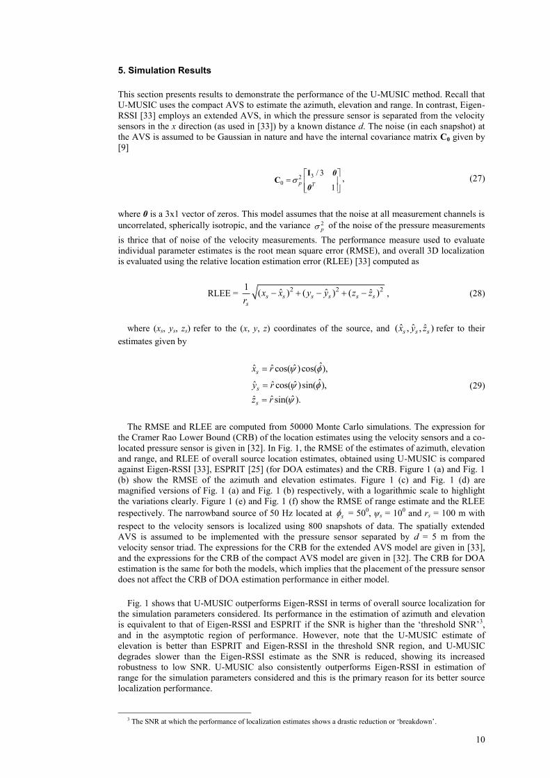
Fig 2: Sensitivity of estimate of elevation to the azimuth estimate vs. error in azimuth angle estimation, (xs, ys, zs) = (63.3,

75.4, 17.4) m, SNR = -4 dB.

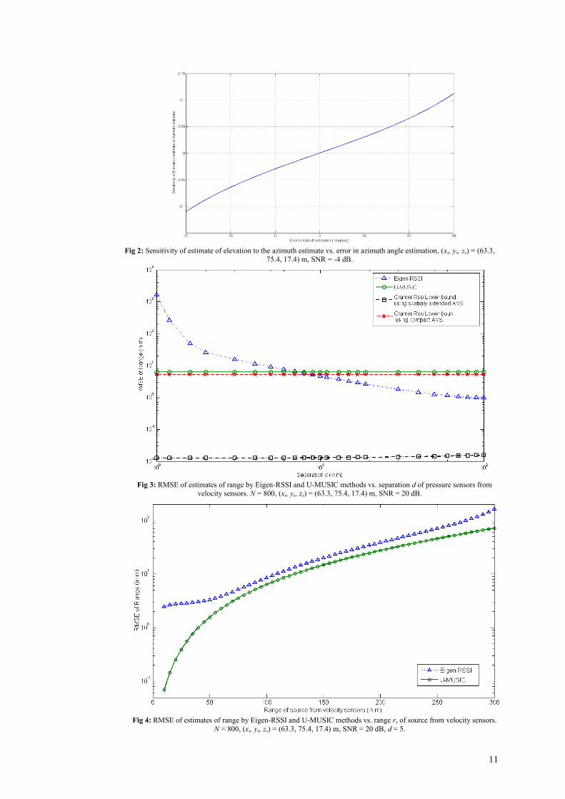
Fig 3: RMSE of estimates of range by Eigen-RSSI and U-MUSIC methods vs. separation d of pressure sensors from

velocity sensors. N = 800, (xs, ys, zs) = (63.3, 75.4, 17.4) m, SNR = 20 dB.

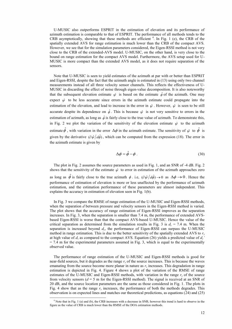
Fig 4: RMSE of estimates of range by Eigen-RSSI and U-MUSIC methods vs. range rs of source from velocity sensors.

N = 800, (xs, ys, zs) = (63.3, 75.4, 17.4) m, SNR = 20 dB, d = 5.

12

U-MUSIC also outperforms ESPRIT in the estimation of elevation and its performance of

azimuth estimation is comparable to that of ESPRIT. The performance of all methods tends to the

CRB asymptotically, showing that these methods are efficient 4. In Fig. 1 (e), the CRB of the

spatially extended AVS for range estimation is much lower than the CRB of the compact AVS.

However, we see that for the simulation parameters considered, the Eigen-RSSI method is not very

close to the CRB of the extended-AVS model. U-MUSIC, on the other hand, is very close to the

bound on range estimation for the compact AVS model. Furthermore, the AVS setup used for U-

MUSIC is more compact than the extended AVS model, as it does not require separation of the

sensors.

Note that U-MUSIC is seen to yield estimates of the azimuth at par with or better than ESPRIT

and Eigen-RSSI, despite the fact that the azimuth angle is estimated in (13) using only two channel

measurements instead of all three velocity sensor channels. This reflects the effectiveness of U-

MUSIC in discarding the effect of noise through eigen-value decomposition. It is also noteworthy

that the subsequent elevation estimate is based on the estimate of the azimuth. One may

expect to be less accurate since errors in the azimuth estimate could propagate into the

estimation of the elevation, and lead to increase in the error in . However, is seen to be still

accurate despite its dependence on . This is because is not very sensitive to errors in the

estimation of azimuth, as long as is fairly close to the true value of azimuth. To demonstrate this,

in Fig. 2 we plot the variation of the sensitivity of the elevation estimate to the azimuth

estimate , with variation in the error in the azimuth estimate. The sensitivity of to is

given by the derivative ˆˆ( ) d , which can be computed from the expression (18). The error in

the azimuth estimate is given by

ˆ . (30)

The plot in Fig. 2 assumes the source parameters as used in Fig. 1, and an SNR of -4 dB. Fig. 2

shows that the sensitivity of the estimate to error in estimation of the azimuth approaches zero

as long as is fairly close to the true azimuth . i.e, ˆˆ( ) 0 d as 0 . Hence the

performance of estimation of elevation is more or less unaffected by the performance of azimuth

estimation, and the estimation performance of these parameters are almost independent. This

explains the accuracy in estimation of elevation seen in Fig. 1(b).

In Fig. 3 we compare the RMSE of range estimation of the U-MUSIC and Eigen-RSSI methods,

when the separation d between pressure and velocity sensors in the Eigen-RSSI method is varied.

The plot shows that the accuracy of range estimation of Eigen-RSSI improves as the separation

increases. In Fig. 3, when the separation is smaller than 7.4 m, the performance of extended AVS-

based Eigen-RSSI is worse than that the compact AVS-based U-MUSIC. Hence the value of the

critical separation as determined from the simulation results in Fig. 3 is dc = 7.4 m. When the

separation is increased beyond dc, the performance of Eigen-RSSI can surpass the U-MUSIC

method in range estimation. This is due to the better sensitivity of the spatially extended AVS to rs

at high value of d, as compared to the compact AVS. Equation (26) yields a predicted value of dc’

= 7.4 m for the experimental parameters assumed in Fig. 3, which is equal to the experimentally

observed value.

The performance of range estimation of the U-MUSIC and Eigen-RSSI methods is good for

near-field sources, but it degrades as the range rs of the source increases. This is because the waves

emanating from the source become more planar in nature as rs increases. This degradation in range

estimation is depicted in Fig. 4. Figure 4 shows a plot of the variation of the RMSE of range

estimates of the U-MUSIC and Eigen-RSSI methods, with variation in the range rs of the source

from velocity sensors (d = 5 m for the Eigen-RSSI method). The signal is received at an SNR of

20 dB, and the source location parameters are the same as those considered in Fig. 1. The plots in

Fig. 4 show that as the range rs increases, the performance of both the methods degrades. This

observation is on expected lines and matches our theoretical predictions, as equations (24) and (25)

4 Note that in Fig. 1 (a) and (b), the CRB increases with a decrease in SNR; however this trend is hard to observe in the

figure as the value of CRB is much lower than the RMSE of the DOA estimation methods.

13

show that the range sensitivity of both the AVS models decreases as the source moves further

away from the sensors.

Note that since the U-MUSIC method is based on eigen-decomposition similar to MUSIC, it is

effective in the case of finite-variance non-Gaussian noise also [23]. If the environmental noise

follows an alpha-stable noise distribution with infinite variance, the U-MUSIC method can also be

easily adapted for such an environment by using several approaches in the literature, such as

employing fractional order correlation to compute the data correlation matrix and obtain the signal

eigen-vectors [35]. However, since a detailed study on these variations is beyond the scope of this

paper, we wish to point this out as a possible enhancement to U-MUSIC.

Since the extended AVS requires a large separation of the pressure sensor from the velocity

sensors, it no longer possesses the compactness associated with a single sensor. Hence it cannot be

used in applications which require the AVS to be mounted in a confined space. The extended AVS

also requires calibration of this known separation of sensors in a known direction, which is an

additional burden during its deployment. Hence the U-MUSIC method using the compact AVS is

advantageous compared to the extended AVS for source localization, when the compactness of the

sensor system is a priority.

6. Conclusions

This paper presents a novel method called U-MUSIC to localize an acoustic source located in

the near-field using a single AVS. The proposed method provides closed form expressions for the

estimates of source azimuth, elevation and range. Hence it avoids a complex 3-D search for the

location parameters which is required in conventional localization methods. U-MUSIC employs a

compact AVS with co-located pressure and velocity sensors, and is found to perform better than

the method presented by Wu and Wong [33]. Thus U-MUSIC is able to offer better performance

with a more compact AVS setup than that provided by the extended AVS. Furthermore, the

compact AVS configuration does not require calibration of the separated pressure sensor from the

velocity sensors. An accurate expression for the threshold value of separation, below which the

compact AVS yields better performance than the extended AVS, is also derived.

References

1. Abdi, A. et al.: A New Vector Sensor Receiver for Underwater Acoustic Communication. Oceans

2007. pp. 1–10 IEEE (2007).

2. Chen, H., Zhao, J.: Coherent signal-subspace processing of acoustic vector sensor array for DOA estimation of wideband sources. Signal Processing. 85, 4, 837–847 (2005).

3. D’Spain, G.L. et al.: Initial Analysis Of The Data From The Vertical DIFAR Array. OCEANS 92 Proceedings- Mastering the Oceans Through Technology. pp. 346–351 IEEE (1992).

4. D’Spain, G.L. et al.: The simultaneous measurement of infrasonic acoustic particle velocity and

acoustic pressure in the ocean by freely drifting Swallow floats. IEEE Journal of Oceanic

Engineering. 16, 2, 195–207 (1991).

5. Felisberto, P. et al.: Tracking Source azimuth Using a Single Vector Sensor. 2010 Fourth

International Conference on Sensor Technologies and Applications. 416–421 (2010).

6. Hari, V.N. et al.: Narrowband detection in ocean with impulsive noise using an acoustic vector

sensor array. 20th European Signal Processing Conference (EUSIPCO 2012). pp. 1334–1339 IEEE, Bucharest, Romania (2012).

7. Hari, V.N. et al.: Underwater signal detection in partially known ocean using short acoustic vector sensor array. OCEANS 2011 IEEE - Spain. pp. 1–9 IEEE, Santander (2011).

8. Hawkes, M., Nehorai, A.: Acoustic vector-sensor beamforming and Capon direction estimation. IEEE Transactions on Signal Processing. 46, 9, 2291–2304 (1998).

14

9. Hawkes, M., Nehorai, A.: Acoustic vector-sensor correlations in ambient noise. IEEE Journal of Oceanic Engineering. 26, 3, 337–347 (2001).

10. He, J., Liu, Z.: Efficient underwater two-dimensional coherent source localization with linear vector-hydrophone array. Signal Processing. 89, 9, 1715–1722 (2009).

11. He, J., Liu, Z.: Two-dimensional direction finding of acoustic sources by a vector sensor array using the propagator method. Signal Processing. 88, 10, 2492–2499 (2008).

12. Hung, H.-S. et al.: 3-D MUSIC with polynomial rooting for near-field source localization. 1996

IEEE International Conference on Acoustics, Speech, and Signal Processing Conference Proceedings. pp. 3065–3068 IEEE.

13. Kim, J.H. et al.: Passive ranging sonar based on multi-beam towed array. OCEANS 2000 MTS/IEEE Conference and Exhibition. Conference Proceedings (Cat. No.00CH37158). pp. 1495–1499 IEEE.

14. Lee, C.M. et al.: Efficient algorithm for localising 3-D narrowband multiple sources. IEE Proceedings - Radar, Sonar and Navigation. 148, 1, 23 (2001).

15. Machell, F.W. et al.: Statistical characteristics of ocean acoustic noise processes. In: Wegman, E.J. et

al. (eds.) Topics in Non-Gaussian Signal Processing. pp. 29–57 Springer New York, New York (1989).

16. Nagananda, K.G., Anand, G.V.: Subspace intersection method of high-resolution bearing estimation

in shallow ocean using acoustic vector sensors. Signal Processing. 90, 1, 105–118 (2010).

17. Nehorai, A., Paldi, E.: Acoustic vector-sensor array processing. IEEE Transactions on Signal Processing. 42, 9, 2481–2491 (1994).

18. Porter, M. et al.: The Makai experiment: High frequency acoustics. In: Jesus, S.M. and Rodríguez, O.C. (eds.) ECUA. pp. 9–18 , Carvoerio, Portugal (2006).

19. Santos, P. et al.: Geometric and seabed parameter estimation using a vector sensor array —

Experimental results from Makai experiment 2005. OCEANS 2011 IEEE - Spain. pp. 1–10 IEEE (2011).

20. Santos, P. et al.: Seabed geoacoustic characterization with a vector sensor array. The Journal of the Acoustical Society of America. 128, 5, 2652–63 (2010).

21. Song, A. et al.: Experimental Demonstration of Underwater Acoustic Communication by Vector

Sensors. IEEE Journal of Oceanic Engineering. 36, 3, 454–461 (2011).

22. Song, A. et al.: Time reversal receivers for underwater acoustic communication using vector sensors. OCEANS 2008. pp. 1–10 IEEE (2008).

23. Stoica, P.: MUSIC, maximum likelihood, and Cramer-Rao bound. IEEE Transactions on Acoustics, Speech, and Signal Processing. 37, 5, 720–741 (1989).

24. Swindlehurst, A.L., Kailath, T.: Passive direction-of-arrival and range estimation for near-field sources. Fourth Annual ASSP Workshop on Spectrum Estimation and Modeling. pp. 123–128 IEEE.

25. Tichavsky, P. et al.: Near-field/far-field azimuth and elevation angle estimation using a single vector hydrophone. IEEE Transactions on Signal Processing. 49, 11, 2498–2510 (2001).

26. Weiss, A.J., Friedlander, B.: Range and bearing estimation using polynomial rooting. IEEE Journal of Oceanic Engineering. 18, 2, 130–137 (1993).

27. Wong, K.T.: Acoustic Vector-Sensor FFH “Blind” Beamforming & Geolocation. IEEE Transactions

on Aerospace and Electronic Systems. 46, 1, 444–448 (2010).

15

28. Wong, K.T., Zoltowski, M.D.: Closed-form underwater acoustic direction-finding with arbitrarily

spaced vector hydrophones at unknown locations. IEEE Journal of Oceanic Engineering. 22, 3, 566–575 (1997).

29. Wong, K.T., Zoltowski, M.D.: Extended-aperture underwater acoustic multisource azimuth/elevation

direction-finding using uniformly but sparsely spaced vector hydrophones. IEEE Journal of Oceanic

Engineering. 22, 4, 659–672 (1997).

30. Wong, K.T., Zoltowski, M.D.: Root-MUSIC-based azimuth-elevation angle-of-arrival estimation

with uniformly spaced but arbitrarily oriented velocity hydrophones. IEEE Transactions on Signal Processing. 47, 12, 3250–3260 (1999).

31. Wong, K.T., Zoltowski, M.D.: Self-initiating MUSIC-based direction finding in underwater acoustic particle velocity-field beamspace. IEEE Journal of Oceanic Engineering. 25, 2, 262–273 (2000).

32. Wu, Y.I. et al.: The Acoustic Vector-Sensor’s Near-Field Array-Manifold. IEEE Transactions on Signal Processing. 58, 7, 3946–3951 (2010).

33. Wu, Y.I., Wong, K.T.: Acoustic Near-Field Source-Localization by Two Passive Anchor-Nodes.

IEEE Transactions on Aerospace and Electronic Systems. 48, 1, 159–169 (2012).

34. Xu, Y. et al.: Perturbation analysis of conjugate MI-ESPRIT for single acoustic vector-sensor-based

noncircular signal direction finding. Signal Processing. 87, 7, 1597–1612 (2007).

35. Zha, D., Qiu, T.: Underwater sources location in non-Gaussian impulsive noise environments. Digital Signal Processing. 16, 2, 149–163 (2006).

36. Zhong, X. et al.: Multi-modality likelihood based particle filtering for 2-D direction of arrival

tracking using a single acoustic vector sensor. 2011 IEEE International Conference on Multimedia and Expo. pp. 1–6 IEEE (2011).

37. Zhong, X. et al.: Particle Filtering and Posterior Cramér-Rao Bound for 2-D Direction of Arrival Tracking Using an Acoustic Vector Sensor. IEEE Sensors Journal. 12, 2, 363–377 (2012).

38. Zhong, X., Premkumar, A.B.: Particle Filtering Approaches for Multiple Acoustic Source Detection

and 2-D Direction of Arrival Estimation Using a Single Acoustic Vector Sensor. IEEE Transactions on Signal Processing. 60, 9, 4719–4733 (2012).

39. Zoltowski, M.D., Wong, K.T.: Closed-form eigenstructure-based direction finding using arbitrary

but identical subarrays on a sparse uniform Cartesian array grid. IEEE Transactions on Signal Processing. 48, 8, 2205–2210 (2000).