Embed Size (px)
Citation preview
COMMUN. MATH. SCI. c© 2009 International Press
Vol. 7, No. 4, pp. 1009–1037
A DIFFUSE-INTERFACE APPROACH FOR MODELINGTRANSPORT, DIFFUSION AND ADSORPTION/DESORPTION OF
MATERIAL QUANTITIES ON A DEFORMABLE INTERFACE∗
KNUT ERIK TEIGEN† , XIANGRONG LI‡ , JOHN LOWENGRUB§ , FAN WANG¶, AND
AXEL VOIGT‖
Abstract. A method is presented to solve two-phase problems involving a material quantity onan interface. The interface can be advected, stretched, and change topology, and material can beadsorbed to or desorbed from it. The method is based on the use of a diffuse interface framework, whichallows a simple implementation using standard finite-difference or finite-element techniques. Here,finite-difference methods on a block-structured adaptive grid are used, and the resulting equationsare solved using a non-linear multigrid method. Interfacial flow with soluble surfactants is used asan example of the application of the method, and several test cases are presented demonstrating itsaccuracy and convergence.
Key words. Partial differential equations, diffuse interface, interfacial dynamics, complexgeometry,multigrid, adaptive grid, finite difference, multiphase, adsorption, desorption
AMS subject classifications. 35Q35, 35K05, 35K57, 65Z05, 65M06, 65M50, 65M55, 76Txx,82C24.
1. Introduction Many problems in the biological, physical and engineeringsciences involve systems of equations that need to be solved in evolving domains withcomplex shapes. In addition, the solutions in the bulk domain may couple with thesurface through adsorption of mass from the bulk to the surface and desorption from thesurface to the bulk. Furthermore, the evolution of the domain boundary may dependon the distribution of the surface concentration through the modification of interfacialforces. Surfactants are a classic example where the amphiphilic organic compounds mayadsorb to and desorb from a liquid/liquid or liquid/gas interface and lower the surfacetension on the interface. Thus, inhomogeneous distribution of surfactants producesMarangoni forces — tangential forces along the interface — that affect the dynamics;surfactants play important roles in vortex pair interaction (e.g., [86, 34]), fingering (e.g.,[84, 63]) and drop break-up and coalescence (e.g., [35, 36, 48, 32]). Other examplesinclude biomembranes where transmembrane proteins play an important role in intra-and extra-cellular dynamics (e.g., [46, 2, 51, 29]), epitaxially grown thin films whereadsorbing/desorbing adatoms affect the dynamics and coarsening of the thin film (e.g.,[23, 81, 52]), and electrochemical dissolution of binary alloys where one component isremoved selectively and dissolved in an electrolyte solution (e.g., [19, 15]).
∗Received: June 4, 2009; accepted (in revised version): August 26, 2009. Communicated by ChunLiu.†Department of Energy and Process Engineering, Norwegian University of Science and Technology,
7491 Trondheim, Norway ([email protected])‡Department of Mathematics, University of California, Irvine, Irvine CA-92697, USA
([email protected])§Department of Mathematics, University of California, Irvine, Irvine CA-92697, USA (lowen-
[email protected])¶Department of Mathematics, University of California, Irvine, Irvine CA-92697, USA
([email protected])‖Department of Mathematics, Technische Universitt Dresden, 01062 Dresden, Germany
1009
1010 COUPLED INTERFACIAL AND BULK MASS TRANSPORT
From a numerical point of view, solving a coupled bulk/surface system of equationson a moving, complex domain is highly challenging; the domain boundary maystretch, break-up or coalesce with other interfaces. Adsorption of mass to, anddesorption of mass from, the interfaces poses another challenge. Furthermore, thesurface concentration may only be soluble in either the exterior or interior of thedomain (e.g., amphiphilic nature of surfactants). The available numerical methods forsolving these problems can roughly be divided into two categories: interface trackingand interface capturing methods. Interface tracking methods use either through aseparate grid for the interface, or a set of interconnected points to mark the interface.For example, boundary integral methods use a surface mesh to track the interface.In the context of surfactants, a boundary integral method for studying the effect ofinsoluble surfactants on drop deformation was developed in [82]. This method wasextended to arbitrary viscosity ratios in [67], and to soluble surfactants in [66]. Anothertracking method is the front-tracking method, where a fixed grid is used to computethe flow, while a set of connected marker particles is used to track the interface and anyinterfacial quantities. A front-tracking method for insoluble surfactants was developedin [39], and this method was extended to handle soluble surfactants in [91] and [69].Lagrangian approaches are typically very accurate, but can be relatively complicatedto implement, especially in three dimensions and for problems involving topologicalchanges.
In interface capturing methods, the interface is not tracked explicitly, but insteadis implicitly defined through a regularization of the interface. This means that thesolution of the problem can be done independently of the underlying grid, whichgreatly simplifies gridding, discretization, and handling of topological changes. Forexample, a volume-of-fluid (VOF) method for insoluble surfactants was developed in[75]. A more general method which allows non-linear equations of state for surfacetension was then developed in [38]. A level-set method for solving the surfactantequation was presented in [89], and later coupled to an external flow solver in [88]. Analternative approach tracking and approach was developed in [90, 32], using the so-called Arbitrary Lagrangian-Eulerian (ALE) method. An immersed interface boundarymethod for interfacial flows with insoluble surfactants was recently developed in [47].In the context of thin films, a level-set method for the simulating the motion of thinfilms under surface diffusion with free adatoms was developed in [81]. In addition,an immersed interface method was developed to simulate electrodeposition in anevolving complex domain [77]. Level-set methods for solving more general equationson implicitly defined, but stationary, surfaces have also been developed in [5, 30].
Other approaches for solving equations in complex domains include fictitiousdomain methods (e.g., [27, 28, 65, 31, 70, 12, 74, 72, 56, 33]), immersed interfacemethods (e.g., [49, 54, 37]), modified finite volume/embedded boundary/cut-cellmethods (e.g., [41, 64, 62, 40, 42, 76, 59]) and ghost fluid methods (e.g., [20, 24, 25,26, 60, 61]). All these methods, however, require non-standard tools typically notavailable in standard finite element and finite difference software packages.
The diffuse-interface, or phase-field, method represents yet another approach forsimulating solutions of equations in complex, evolving domains. In this method, whichwe follow here, the complex domain is represented implicitly by a a phase-field function,which is an approximation of the characteristic function of the domain. The domainboundary is replaced by a narrow diffuse interface layer such that the phase-fieldfunction rapidly transitions from one inside the domain to zero in the exterior of thedomain. The boundary of the domain can thus be represented as an isosurface of
K.E. TEIGEN, X. LI, J. LOWENGRUB, F. WANG, AND A. VOIGT 1011
the phase-field function. The bulk and surface PDEs are then extended on a larger,regular domain with additional terms that approximate the adsorption-desorption fluxboundary conditions and source terms for the bulk and surface equations respectively.Standard finite-difference or finite-element methods may be used. Here, we focus on afinite difference approach.
The diffuse interface method, which has a long history in the theory of phasetransitions dating back to van der Waals (e.g., [79, 3]), was used in [46] to studydiffusion inside a cell with zero Neumann boundary conditions at the (stationary)cell-boundary (see also [8, 9]), and later was used to simulate electrical waves in theheart [21]. This approach has been extended [51] to simulate coupled bulk diffusionwith an ordinary-differential equation description of reaction-kinetics on the boundingsurface of a stationary domain to simulate membrane-bound Turing patterns. Morerecently, general diffuse-interface methods have been developed for solving PDEs onstationary surfaces [73], evolving surfaces [13, 14, 16, 17] and for solving PDEs incomplex evolving domains with Dirichlet, Neumann and Robin boundary conditions[53].
As shown in the previous paragraphs, bulk/surface problems are important in awide range of areas. Here, we combine and refine previous work on diffuse-interfacemethods to develop a new method for solving coupled bulk/surface problems on general,evolving domains. The method is very simple compared to other methods, and canhandle advection, diffusion and adsorption/desorption in a straight-forward manner.Matched asymptotic expansions are used to demonstrate that the diffuse interfacesystem converges to the original sharp interface equations as the interface thicknesstends to zero. The use of a non-linear multigrid method and block-structured, adaptivegrids also make the method computationally efficient. We present several test casesdemonstrating the accuracy and convergence of the proposed method.
The paper is organized as follows. In section 2, the governing equations for thesurface concentration and the bulk concentration are introduced, and the interfacerepresentation presented. Section 3 presents an asymptotic analysis of the proposedmethod. Section 4 then details the numerical implementation. In section 5, theperformance of the numerical method is evaluated on a set of test cases. Finally,section 6 contains conclusions and discussions of future work.
2. Mathematical formulation
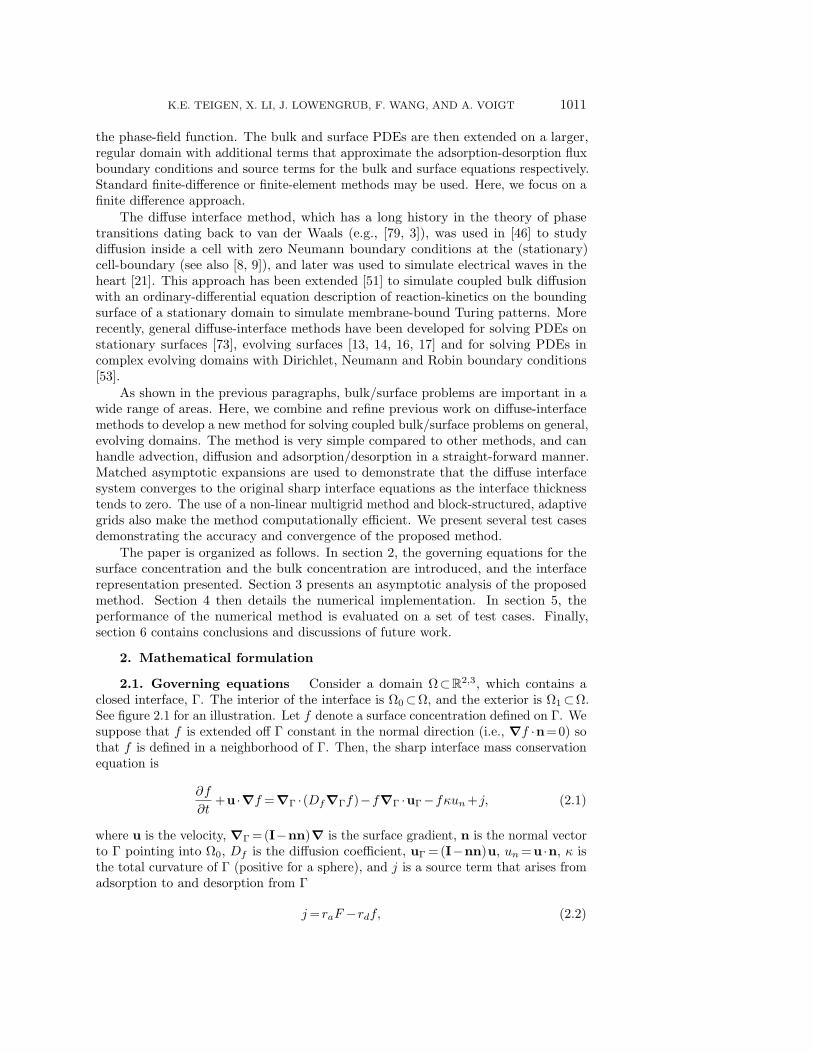
2.1. Governing equations Consider a domain Ω⊂R2,3, which contains aclosed interface, Γ. The interior of the interface is Ω0⊂Ω, and the exterior is Ω1⊂Ω.See figure 2.1 for an illustration. Let f denote a surface concentration defined on Γ. Wesuppose that f is extended off Γ constant in the normal direction (i.e., ∇f ·n= 0) sothat f is defined in a neighborhood of Γ. Then, the sharp interface mass conservationequation is
∂f
∂t+u ·∇f =∇Γ ·(Df∇Γf)−f∇Γ ·uΓ−fκun+j, (2.1)
where u is the velocity, ∇Γ = (I−nn)∇ is the surface gradient, n is the normal vectorto Γ pointing into Ω0, Df is the diffusion coefficient, uΓ =(I−nn)u, un=u ·n, κ isthe total curvature of Γ (positive for a sphere), and j is a source term that arises fromadsorption to and desorption from Γ
j= raF −rdf, (2.2)
1012 COUPLED INTERFACIAL AND BULK MASS TRANSPORT
Ω0
Ω1
Γ
Fig. 2.1: Illustration of the mathematical domain.
where ra and rd are adsorption and desorption coefficients, respectively, and F is thebulk concentration (evaluated immediately adjacent to Γ). Note that in the context ofsurfactants, the interface may become saturated and instead one may use
j= raF (f∞−f)−rdf, (2.3)
where f∞ is the maximum interface concentration. An equivalent formulation is
∂f
∂t+∇Γ ·(uf) =∇Γ ·(Df∇Γf)+j. (2.4)
We refer the reader also to [11] for further discussion of formulations involving interfacialtransport using constant normal extensions and to [38] for Eulerian formulations ofthe dynamics of surface concentrations.
Assume that the surface concentration f is soluble in Ω1, but not in Ω0. Then,define the bulk concentration in Ω1 to be F , which evolves according to the bulk massconservation equation
∂F
∂t+∇·(Fu) =DF∇2F in Ω1, (2.5)
with the boundary condition at Γ
DF∇F ·n=−j on Γ. (2.6)
Note that if the surface concentration were soluble in Ω0, then an additional massconservation equation would need to be posed. Our formulation is sufficiently generalto handle this case.
Next, we consider a distribution formulation of equation (2.4) by introducing asurface delta function δΓ, such that∫
Γ
f dΓ =∫
Ω
fδΓ dΩ, (2.7)
K.E. TEIGEN, X. LI, J. LOWENGRUB, F. WANG, AND A. VOIGT 1013
where Ω = Ω1∪Ω0 (actually the above equation holds for any domain Ω that containsΓ). The mass conservation equation may be rewritten accordingly as
∂
∂t(f δΓ)+∇·(f δΓu) =∇·(δΓDf∇f)+δΓj. (2.8)
This distribution formulation formally holds in Ω.Analogously, the bulk equation (2.5) may be extended to hold in Ω in distribution
form. Introducing the Heaviside function
H=
1 in Ω1,0 in Ω0,
(2.9)
the bulk concentration equation (2.5) and boundary condition (2.6) may be reformu-lated as
∂
∂t(HF )+∇·(HF u) =DF∇·(H∇F )−δΓj, (2.10)
where the boundary condition has been included as a singular source term following[53].
2.2. Interface representation A phase-field function c may be used to ap-proximate the characteristic function of Ω1. Let
c(x,t) =12
[1+tanh
(r(x,t)2√
2ε
)], (2.11)
where ε is a small parameter related to the interface thickness and r(x,t) is a signeddistance function to Γ (positive in Ω1). The position of the interface may be taken tobe Γ(t) =x∈Ω | c(x,t) = 1/2. To evolve c, one may evolve r by
∂r
∂t+v ·∇r= 0, (2.12)
where v is an extension of u off the interface which is constant in the normal direction[1]. Alternatively, an advective Cahn-Hilliard equation can be used,
∂c
∂t+u ·∇c=∇·(M(c)∇µ), (2.13)
µ=g′(c)−ε2∇2c, (2.14)
where µ is a chemical potential. Here, we take g(c)= 14c
2(1−c)2 as the double wellpotential. Note that this polynomial energy does not constrain c∈ [0,1] but thedeviation from this interval is typically O(ε) at most. Alternative choices (e.g., double-obstacle [6, 7] or logarithmic potentials [4]) may be used that do constrain c∈ [0,1].The mobility M is localized on the interface and is taken to be M(c) =
√4g(c). This
equation is fourth-order and nonlinear and thus requires specialized numerical methodsto solve in an efficient manner. This is discussed further in section 4.
2.3. Regularized delta and Heaviside functions In order to evaluate equa-tion (2.8) and equation (2.10) numerically, regularizations of the surface delta functionand Heaviside function are needed. In the phase-field context, several definitions of
1014 COUPLED INTERFACIAL AND BULK MASS TRANSPORT
the delta function are available from the literature. In this work, the approximationfrom [73],
δΓ≈3√
2εB(c), B(c) = c2(1−c)2, (2.15)
is used for the surface equation. Note that other choices may be used [17]. For theboundary condition in the bulk equation, the approximation
δΓ≈|∇c| (2.16)
is used, which avoids additional scaling issues in the equation [53]. Further, theregularized Heaviside function is simply taken to be [53]
H(c)≈ c. (2.17)
The final system of equations can now be summarized as
∂
∂t(B(c)f)+∇·(B(c)fu) =∇·(DfB(c)∇f)+B(c)j, (2.18)
∂
∂t(cF )+∇·(cF u) =DF∇·(c∇F )−|∇c|j. (2.19)
3. Asymptotic analysis In this section, the method of matched asymptoticexpansions is used to provide a formal justification for the diffuse interface approach.To make the system slightly more general, we may add reaction terms to the bulkand surface equations, i.e., Rf (f) and RF (F ) may be added to equations (2.18) and(2.19) respectively. In this approach, the domain Ω is separated into two regions —the regions far from Γ (outer region, i.e., the portions of Ω1 and Ω0 away from Γ) andthe region near Γ (inner region). In each region, the variables are expanded in powersof the diffuse interface thickness. In the outer region, the variables are expanded as
c(x,t) = c0(x,t)+εc1(x,t)+ .. ., (3.1)
and analogously for the other variables. In the region near Γ, we introduce a newcoordinate system.
3.1. New Coordinate Introduce the following local normal-tangential coor-dinate system with respect to the curve Γ. Let Γ=X(s,t)=(X(s,t),Y (s,t),Z(s,t)),where s=(s1,s2) is a parametrization of the surface and t is time. Let r= r(x;ε) bethe signed distance along the normal from a point x to Γ, and is positive when outsideΓ (i.e. in Ω1). Then, if Γ is smooth, there exists a neighborhood
Uε :=x∈Ω : |r(x,ε)|<ρ
of Γ for some 0<ρ1, such that the local coordinate transformation from (x,y,z)to (r,s1,s2) is valid, e.g., x=X(s,t)+rn(s,t). Near the interface, we introduced astretched normal coordinate z= r
ε . Note that as ε→0, the inner region extends from−∞<z<∞. We then assume that the variables may be expanded in regular powerseries in ε in the stretched coordinate system:
c(x,t) =C(z,s,t) =C0(z,s,t)+εC1(z,s,t)+ .. ., (3.2)
K.E. TEIGEN, X. LI, J. LOWENGRUB, F. WANG, AND A. VOIGT 1015
and analogously for the other variables. Furthermore, in this coordinate system wehave
∂t=−ε−1V0∂z+∂t+O(ε), (3.3)
∇= ε−1n∂z+∇Γ +O(ε), (3.4)
where V0 is the leading term of the normal velocity of Γ.
3.2. Matching Condition Assuming that there is an overlapping region whereboth the inner and outer expansions are valid, we may write the outer expansion inthe local coordinate system as
c(x,t) = c(r,s,t) = c0(r,s,t)+εc1(r,s,t)+ .. ., (3.5)
and analogously for the other variables. Matching the inner and outer expansions inthis region, the following matching conditions hold [10, 71, 22]
limr→0±
F0 = limz→±∞
F0, (3.6)
limr→0±
f0 = limz→±∞
f0, (3.7)
limr→0±
n ·∇F0 = limz→±∞
∂zF1, (3.8)
limz→±∞
∂zF0 = 0. (3.9)
Analogous matching conditions hold for the other variables.
3.3. Bulk Equation
3.3.1. Outer expansion The O(ε0) term of equation (2.19) gives:
∂F0
∂t+∇ ·(F0u0) =∇ ·(DF∇F0)+RF (F0). (3.10)
Thus at leading order equation (2.5), with the reaction term, is recovered. To determinethe boundary conditions on Γ, we match with the inner expansion.
3.3.2. Inner expansion At O(ε−2), we obtain
∂z(C0DF∂zF0) = 0, (3.11)
which implies ∂zF0 = 0. At O(ε−1) we obtain(UN,0− V0
)∂z
(C0F0
)=∂z(C0DF∂zF1)+
(raF0−rdf0
)∂zC0. (3.12)
Since UN,0 = V0 by the asymptotic analysis of the advective Cahn-Hilliard equation[58], F0 is independent of z and, as we show below, f0 is also independent of z, wemay integrate equation (3.12) and use that
∫ +∞−∞ ∂zC0 dz=1, again taken from [58],
to obtain
DF limz→+∞
∂zF1 =−(raF0−rdf0). (3.13)
Together with equation (3.8), we therefore recover the Neumann boundary condition(2.6) for the outer solution at leading order
DF limr→0+
n ·∇F0 =DF limz→+∞
∂zF1 =−(raF0−rdf0), (3.14)
where we have set f0 =f0 since f0 is independent of z. Next, we turn to the surfaceconcentration equation.
1016 COUPLED INTERFACIAL AND BULK MASS TRANSPORT
3.4. Surface Equation Here, we only focus on the inner expansion since theequation is localized around the interface. At O(ε−2), we obtain
∂z
(DfB(C0)∂z f0
)= 0, (3.15)
which implies ∂z f0 = 0, as claimed above. The O(ε−1) term gives
0 =∂z(B(C0)∂z f1), (3.16)
where we have used that UN,0 = V0. Equation (3.16) implies that ∂z f1 =0 also. AtO(ε0), we obtain
∂t(B(C0)f0)+∇Γ ·(B(C0)f0U0
)=∂z(DfB(C0)∂z f2)+∇Γ ·
(DfB(C0)∇Γf0
)+B(C0)(raF0−rdf0)+B(C0)Rf (f0).
(3.17)
Since f0 is independent of z, we may integrate equation (3.17) in z from −∞ to +∞,and divide by
∫ +∞−∞ B(C0)dz>0 to obtain
∂tf0 +∇Γ ·(f0u0) =∇Γ ·(Df∇Γf0) = raF0−rdf0 +Rf (f0), (3.18)
where we taken f0 =f0, F0 =F0 and we also have assumed that UΓ,0 is independent ofz (which implies there is no jump in velocity across Γ) so that we may write U0 =u0.Thus, equation (2.4), with the reaction term, is recovered at leading order.
4. Numerical methods This section briefly describes the numerical methodsused to solve the above equations. The algorithm follows the one developed in [87]. Inparticular, the equations are discretized using finite differences in space and a semi-implicit time discretization. A block-structured, adaptive grid is used to increase theresolution around the interface in an efficient manner. The nonlinear equations at theimplicit time level are solved using a non-linear Adaptive Full Approximation Scheme(AFAS) multigrid algorithm. For a detailed discussion of the adaptive algorithm andthe multigrid solver, the reader is referred to [87].
The equations are discretized on a rectangular domain. The surface concentration,the bulk concentration, the phase-field function and the chemical potential are definedat the cell-centers, while the velocity components are defined on cell-edges.
Special care has to be taken for the temporal discretization. The Cahn-Hilliardsystem is fourth order in space, and requires the use of an implicit method to avoidsevere limitations in the time step. Here, Crank-Nicholson type schemes are used [45],
ck+1−ck
∆t=− 1
2[∇d ·(uk+1ck+1)+∇d ·(ukck)
]+
12[∇d ·(Mk+1∇dµ
k+1)+∇d ·(Mk∇dµk)],
(4.1)
µk+1 =g′(ck+1)−ε2∇2dck+1. (4.2)
In [45, 87] this approach was shown to be robust and efficient. The equations for
K.E. TEIGEN, X. LI, J. LOWENGRUB, F. WANG, AND A. VOIGT 1017
surface concentration and bulk concentration are discretized in a similar fashion,
δk+1Γ fk+1−δkΓfk
∆t=− 1
2[∇d ·(uk+1δk+1
Γ fk+1)+∇d ·(ukδkΓfk)]
+Df
2[∇d ·(δk+1
Γ ∇dfk+1)+∇d ·(δkΓ∇df
k)]
+12[δk+1Γ jk+1 +δkΓj
k],
(4.3)
Hk+1F k+1−HkF k
∆t=− 1
2[∇d ·(uk+1Hk+1F k+1)+∇d ·(ukHkF k)
]+Df
2[∇d ·(Hk+1∇dF
k+1)+∇d ·(Hk∇dFk)]
+12[|∇dc
k+1|jk+1 + |∇dck|jk
],
(4.4)
where, in the above equations, we set δk+1Γ =B(ck+1)+α and Hk+1 =
√(ck+1)2 +α2,
with α being a small parameter (α= 10−6) that is used to ensure that division by zerodoes not occur; the results are found to be quite insensitive to the precise choice ofα provided it is sufficiently small. The operator ∇d represents the standard second-order finite-difference discretization. The convective terms of the form ∇·(uφ) arediscretized using the third-order WENO reconstruction method [78, 55]. The WENOreconstruction method has the advantage that it handles steep gradients well, whichmay occur in the type of dynamics described in this work. Additionally, fewer gridpoints are needed to achieve a high order solution. This is particularly important forthe efficiency of the adaptive grid, because fewer ghost cell values have to be calculatedat the boundaries of each grid block.
Homogeneous Neumann far-field boundary conditions are prescribed for all vari-ables. This is imposed by introducing a set of ghost cells around the domain. Theseghost cells are updated before every smoothing operation.
The AFAS multigrid algorithm is used to solve the discretized equations at everytime step. The full description of the AFAS multigrid method will not be given here,the details can be found in [87] and in the reference text [85]. The ideal run-timecomplexity of this algorithm is optimal, i.e., O(N) where N is the number of grid points.The present implementation achieves this complexity, which is shown in section 5.6.
5. Code validation
5.1. Surface diffusion on a stationary circle First, a problem without bulkconcentration is considered. This tests the validity of the diffuse interface representationof the surface equation, and of the correct implementation of the diffusion term.
Consider a stationary circle of radius R, with an initial surface concentration givenby
f0(θ) =12
(1−cosθ), (5.1)
where θ denotes the angle measured in the counter-clockwise direction from the y-axis.The surface concentration equation can now be written in polar coordinates as
∂f(θ,t)∂t
=Df
R2
∂2f(θ,t)∂θ2
, (5.2)
1018 COUPLED INTERFACIAL AND BULK MASS TRANSPORT
with initial condition f0 and periodic boundary condition in the θ-direction. Thisequation can be solved analytically, yielding
f(θ,t) =12
(1−e−
Df
R2 tcosθ). (5.3)
A series of simulations are performed comparing the numerical solution to theanalytical solution. The computational domain chosen for the simulations is [−2,2]×[−2,2] and a circle with radius R=1 is placed in the center of the domain. Thephase-field function is initialized by
c(x,y) =12
[1−tanh
(√x2 +y2−R
2√
2ε
)]. (5.4)
The initial surface concentration is given by the analytical solution, and the time stepis ∆t= 1×10⁻².
In the numerical code, the surface concentration is defined at grid points near theinterface. To enable a direct comparison with the analytical solution, the concentrationat the interface is needed. This is done by using a marching squares algorithm (see e.g.[57]) to generate a set of points at the 0.5 isocontour of the phase-field function. Bilinearinterpolation is then used to interpolate the grid values of the surface concentrationto these interface points. Note that this will introduce extra uncertainties, so theabsolute errors given later may not be exact values. The order of convergence resultsshould not be affected by this.
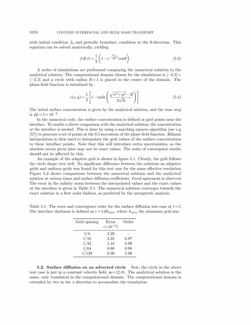
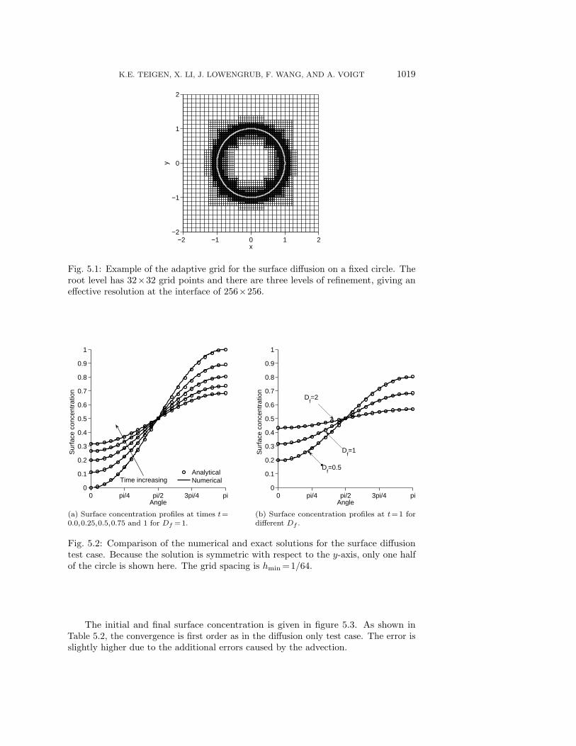
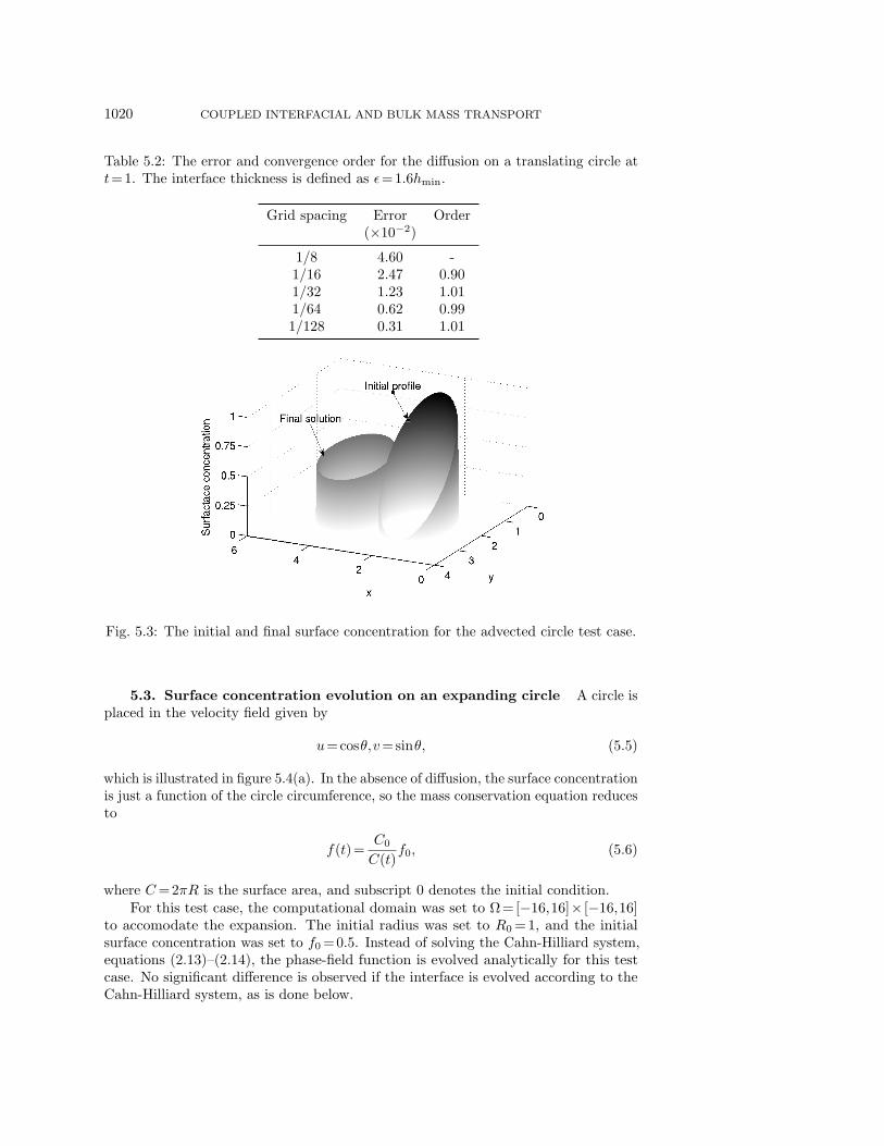
An example of the adaptive grid is shown in figure 5.1. Clearly, the grid followsthe circle shape very well. No significant difference between the solutions on adaptivegrids and uniform grids was found for this test case for the same effective resolution.Figure 5.2 shows comparisons between the numerical solution and the analyticalsolution at various times and surface diffusion coefficients. Good agreement is observed.The error in the infinity norm between the interpolated values and the exact valuesat the interface is given in Table 5.1. The numerical solution converges towards theexact solution in a first order fashion, as predicted by the asymptotic analysis.
Table 5.1: The error and convergence order for the surface diffusion test case at t= 1.The interface thickness is defined as ε= 1.6hmin, where hmin the minimum grid size.
Grid spacing Error Order(×10−2)
1/8 4.29 -1/16 2.35 0.871/32 1.18 0.991/64 0.60 0.981/128 0.30 1.00
5.2. Surface diffusion on an advected circle Now, the circle in the abovetest case is put in a constant velocity field, u=(2,0). The analytical solution is thesame, only translated in the computational domain. The computational domain isextended by two in the x-direction to accomodate the translation.
K.E. TEIGEN, X. LI, J. LOWENGRUB, F. WANG, AND A. VOIGT 1019
−2 −1 0 1 2−2
−1
0
1
2
x
y
Fig. 5.1: Example of the adaptive grid for the surface diffusion on a fixed circle. Theroot level has 32×32 grid points and there are three levels of refinement, giving aneffective resolution at the interface of 256×256.
0 pi/4 pi/2 3pi/4 pi0
0.1
0.2
0.3
0.4
0.5
0.6
0.7
0.8
0.9
1
Angle
Sur
face
con
cent
ratio
n
AnalyticalNumericalTime increasing
(a) Surface concentration profiles at times t=0.0,0.25,0.5,0.75 and 1 for Df = 1.
0 pi/4 pi/2 3pi/4 pi0
0.1
0.2
0.3
0.4
0.5
0.6
0.7
0.8
0.9
1
Angle
Sur
face
con
cent
ratio
n
Df=2
Df=1
Df=0.5
(b) Surface concentration profiles at t=1 fordifferent Df .
Fig. 5.2: Comparison of the numerical and exact solutions for the surface diffusiontest case. Because the solution is symmetric with respect to the y-axis, only one halfof the circle is shown here. The grid spacing is hmin = 1/64.
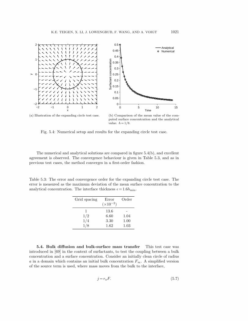
The initial and final surface concentration is given in figure 5.3. As shown inTable 5.2, the convergence is first order as in the diffusion only test case. The error isslightly higher due to the additional errors caused by the advection.
1020 COUPLED INTERFACIAL AND BULK MASS TRANSPORT
Table 5.2: The error and convergence order for the diffusion on a translating circle att= 1. The interface thickness is defined as ε= 1.6hmin.
Grid spacing Error Order(×10−2)
1/8 4.60 -1/16 2.47 0.901/32 1.23 1.011/64 0.62 0.991/128 0.31 1.01
Fig. 5.3: The initial and final surface concentration for the advected circle test case.
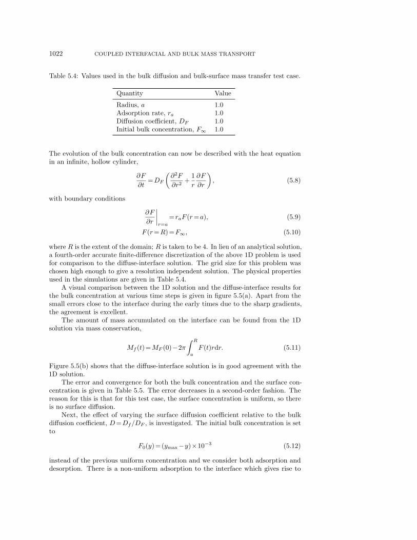
5.3. Surface concentration evolution on an expanding circle A circle isplaced in the velocity field given by
u= cosθ,v= sinθ, (5.5)
which is illustrated in figure 5.4(a). In the absence of diffusion, the surface concentrationis just a function of the circle circumference, so the mass conservation equation reducesto
f(t) =C0
C(t)f0, (5.6)
where C= 2πR is the surface area, and subscript 0 denotes the initial condition.For this test case, the computational domain was set to Ω=[−16,16]× [−16,16]
to accomodate the expansion. The initial radius was set to R0 =1, and the initialsurface concentration was set to f0 = 0.5. Instead of solving the Cahn-Hilliard system,equations (2.13)–(2.14), the phase-field function is evolved analytically for this testcase. No significant difference is observed if the interface is evolved according to theCahn-Hilliard system, as is done below.
K.E. TEIGEN, X. LI, J. LOWENGRUB, F. WANG, AND A. VOIGT 1021
x
y
−2 −1 0 1 2−2
−1
0
1
2
(a) Illustration of the expanding circle test case.
0 5 10 150
0.05
0.1
0.15
0.2
0.25
0.3
0.35
0.4
0.45
0.5
TimeS
urfa
ctan
t con
cent
ratio
n
AnalyticalNumerical
(b) Comparison of the mean value of the com-puted surface concentration and the analyticalvalue. h= 1/8.
Fig. 5.4: Numerical setup and results for the expanding circle test case.
The numerical and analytical solutions are compared in figure 5.4(b), and excellentagreement is observed. The convergence behaviour is given in Table 5.3, and as inprevious test cases, the method converges in a first-order fashion.
Table 5.3: The error and convergence order for the expanding circle test case. Theerror is measured as the maximum deviation of the mean surface concentration to theanalytical concentration. The interface thickness ε= 1.6hmin.
Grid spacing Error Order(×10−2)
1 13.6 -1/2 6.60 1.041/4 3.30 1.001/8 1.62 1.03
5.4. Bulk diffusion and bulk-surface mass transfer This test case wasintroduced in [69] in the context of surfactants, to test the coupling between a bulkconcentration and a surface concentration. Consider an initially clean circle of radiusa in a domain which contains an initial bulk concentration F∞. A simplified versionof the source term is used, where mass moves from the bulk to the interface,
j= raF. (5.7)
1022 COUPLED INTERFACIAL AND BULK MASS TRANSPORT
Table 5.4: Values used in the bulk diffusion and bulk-surface mass transfer test case.
Quantity Value
Radius, a 1.0Adsorption rate, ra 1.0Diffusion coefficient, DF 1.0Initial bulk concentration, F∞ 1.0
The evolution of the bulk concentration can now be described with the heat equationin an infinite, hollow cylinder,
∂F
∂t=DF
(∂2F
∂r2+
1r
∂F
∂r
), (5.8)
with boundary conditions
∂F
∂r
∣∣∣∣r=a
= raF (r=a), (5.9)
F (r=R) =F∞, (5.10)
where R is the extent of the domain; R is taken to be 4. In lieu of an analytical solution,a fourth-order accurate finite-difference discretization of the above 1D problem is usedfor comparison to the diffuse-interface solution. The grid size for this problem waschosen high enough to give a resolution independent solution. The physical propertiesused in the simulations are given in Table 5.4.
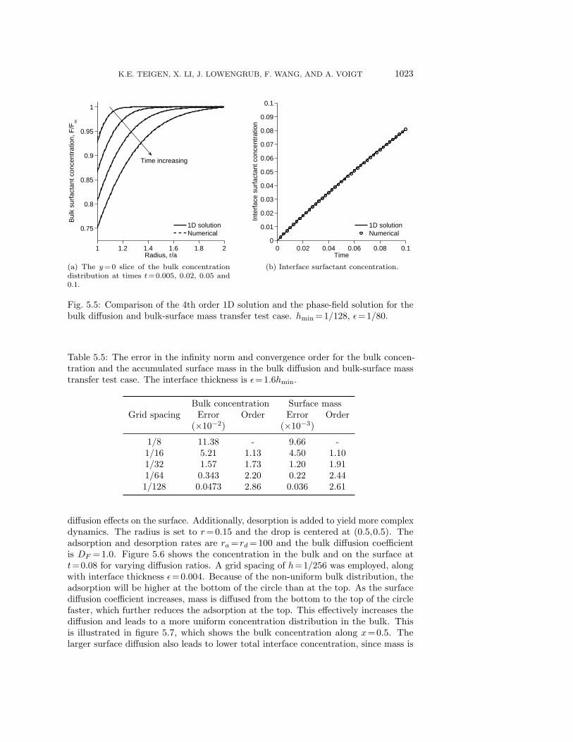
A visual comparison between the 1D solution and the diffuse-interface results forthe bulk concentration at various time steps is given in figure 5.5(a). Apart from thesmall errors close to the interface during the early times due to the sharp gradients,the agreement is excellent.
The amount of mass accumulated on the interface can be found from the 1Dsolution via mass conservation,
Mf (t) =MF (0)−2π∫ R
a
F (t)rdr. (5.11)
Figure 5.5(b) shows that the diffuse-interface solution is in good agreement with the1D solution.
The error and convergence for both the bulk concentration and the surface con-centration is given in Table 5.5. The error decreases in a second-order fashion. Thereason for this is that for this test case, the surface concentration is uniform, so thereis no surface diffusion.
Next, the effect of varying the surface diffusion coefficient relative to the bulkdiffusion coefficient, D=Df/DF , is investigated. The initial bulk concentration is setto
F0(y) = (ymax−y)×10−3 (5.12)
instead of the previous uniform concentration and we consider both adsorption anddesorption. There is a non-uniform adsorption to the interface which gives rise to
K.E. TEIGEN, X. LI, J. LOWENGRUB, F. WANG, AND A. VOIGT 1023
1 1.2 1.4 1.6 1.8 2
0.75
0.8
0.85
0.9
0.95
1
Radius, r/a
Bul
k su
rfac
tant
con
cent
ratio
n, F
/F∞
1D solutionNumerical
Time increasing
(a) The y =0 slice of the bulk concentrationdistribution at times t=0.005, 0.02, 0.05 and0.1.
0 0.02 0.04 0.06 0.08 0.10
0.01
0.02
0.03
0.04
0.05
0.06
0.07
0.08
0.09
0.1
TimeIn
terf
ace
surf
acta
nt c
once
ntra
tion
1D solutionNumerical
(b) Interface surfactant concentration.
Fig. 5.5: Comparison of the 4th order 1D solution and the phase-field solution for thebulk diffusion and bulk-surface mass transfer test case. hmin = 1/128, ε= 1/80.
Table 5.5: The error in the infinity norm and convergence order for the bulk concen-tration and the accumulated surface mass in the bulk diffusion and bulk-surface masstransfer test case. The interface thickness is ε= 1.6hmin.
Bulk concentration Surface massGrid spacing Error Order Error Order
(×10−2) (×10−3)
1/8 11.38 - 9.66 -1/16 5.21 1.13 4.50 1.101/32 1.57 1.73 1.20 1.911/64 0.343 2.20 0.22 2.441/128 0.0473 2.86 0.036 2.61
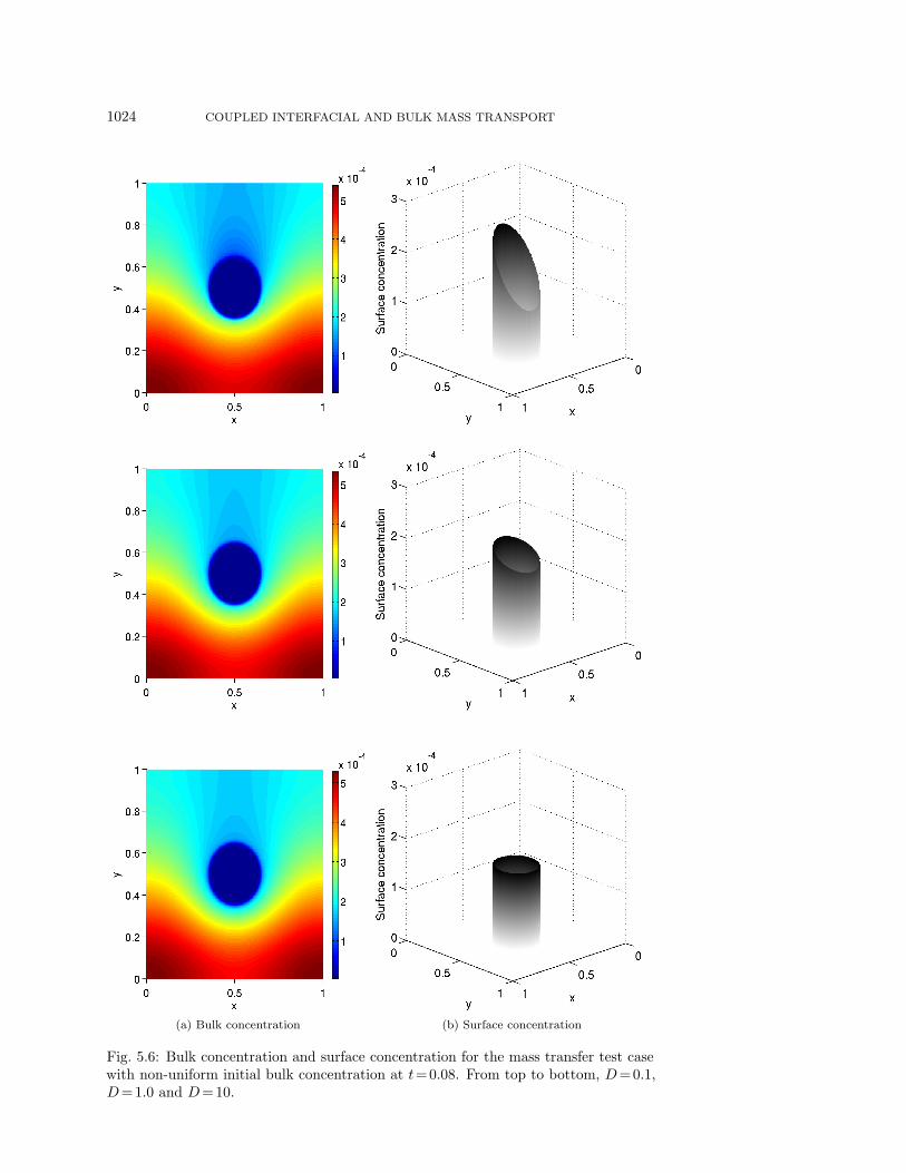
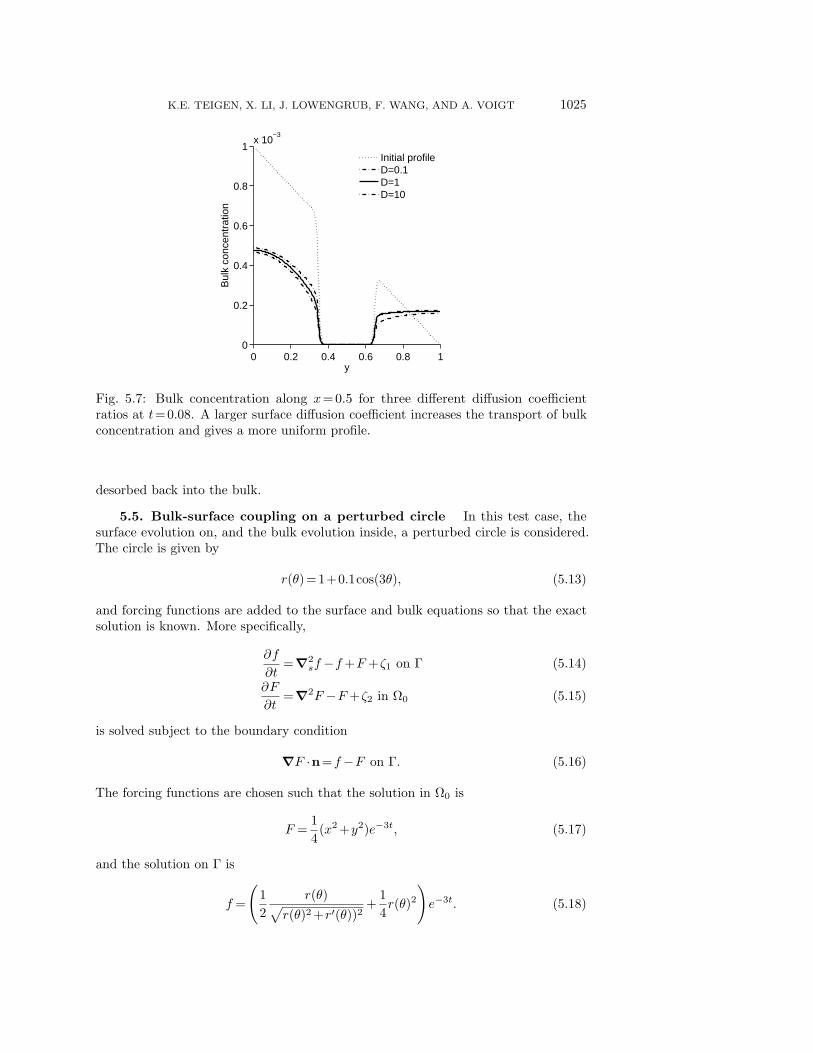
diffusion effects on the surface. Additionally, desorption is added to yield more complexdynamics. The radius is set to r=0.15 and the drop is centered at (0.5,0.5). Theadsorption and desorption rates are ra= rd=100 and the bulk diffusion coefficientis DF =1.0. Figure 5.6 shows the concentration in the bulk and on the surface att= 0.08 for varying diffusion ratios. A grid spacing of h= 1/256 was employed, alongwith interface thickness ε=0.004. Because of the non-uniform bulk distribution, theadsorption will be higher at the bottom of the circle than at the top. As the surfacediffusion coefficient increases, mass is diffused from the bottom to the top of the circlefaster, which further reduces the adsorption at the top. This effectively increases thediffusion and leads to a more uniform concentration distribution in the bulk. Thisis illustrated in figure 5.7, which shows the bulk concentration along x=0.5. Thelarger surface diffusion also leads to lower total interface concentration, since mass is
1024 COUPLED INTERFACIAL AND BULK MASS TRANSPORT
(a) Bulk concentration (b) Surface concentration
Fig. 5.6: Bulk concentration and surface concentration for the mass transfer test casewith non-uniform initial bulk concentration at t= 0.08. From top to bottom, D= 0.1,D= 1.0 and D= 10.
K.E. TEIGEN, X. LI, J. LOWENGRUB, F. WANG, AND A. VOIGT 1025
0 0.2 0.4 0.6 0.8 10
0.2
0.4
0.6
0.8
1x 10
−3
y
Bul
k co
ncen
trat
ion
Initial profileD=0.1D=1D=10
Fig. 5.7: Bulk concentration along x=0.5 for three different diffusion coefficientratios at t= 0.08. A larger surface diffusion coefficient increases the transport of bulkconcentration and gives a more uniform profile.
desorbed back into the bulk.
5.5. Bulk-surface coupling on a perturbed circle In this test case, thesurface evolution on, and the bulk evolution inside, a perturbed circle is considered.The circle is given by
r(θ) = 1+0.1cos(3θ), (5.13)
and forcing functions are added to the surface and bulk equations so that the exactsolution is known. More specifically,
∂f
∂t=∇2
sf−f+F +ζ1 on Γ (5.14)
∂F
∂t=∇2F −F +ζ2 in Ω0 (5.15)
is solved subject to the boundary condition
∇F ·n=f−F on Γ. (5.16)
The forcing functions are chosen such that the solution in Ω0 is
F =14
(x2 +y2)e−3t, (5.17)
and the solution on Γ is
f =
(12
r(θ)√r(θ)2 +r′(θ))2
+14r(θ)2
)e−3t. (5.18)
1026 COUPLED INTERFACIAL AND BULK MASS TRANSPORT
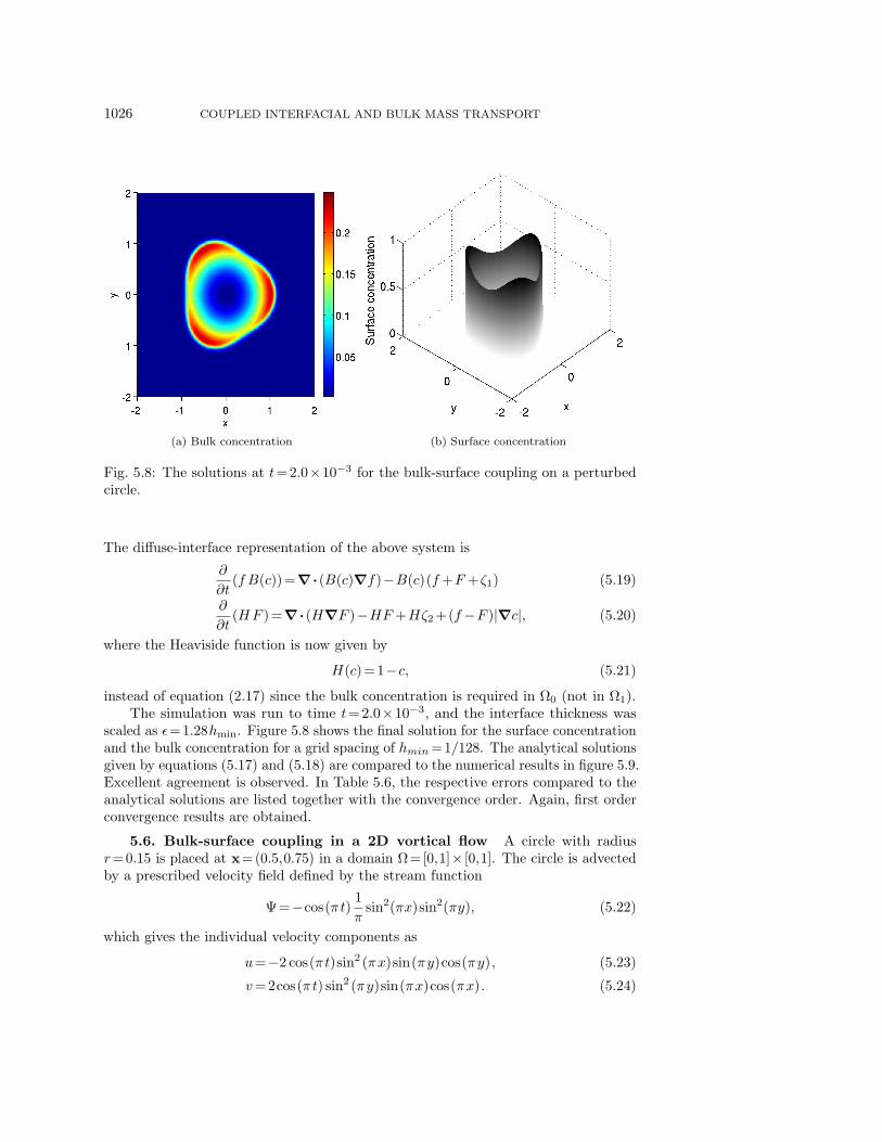
(a) Bulk concentration (b) Surface concentration
Fig. 5.8: The solutions at t= 2.0×10⁻³ for the bulk-surface coupling on a perturbedcircle.
The diffuse-interface representation of the above system is
∂
∂t(f B(c)) =∇·(B(c)∇f)−B(c)(f+F +ζ1) (5.19)
∂
∂t(HF ) =∇·(H∇F )−HF +Hζ2 +(f−F )|∇c|, (5.20)
where the Heaviside function is now given by
H(c) = 1−c, (5.21)
instead of equation (2.17) since the bulk concentration is required in Ω0 (not in Ω1).The simulation was run to time t=2.0×10⁻³, and the interface thickness was
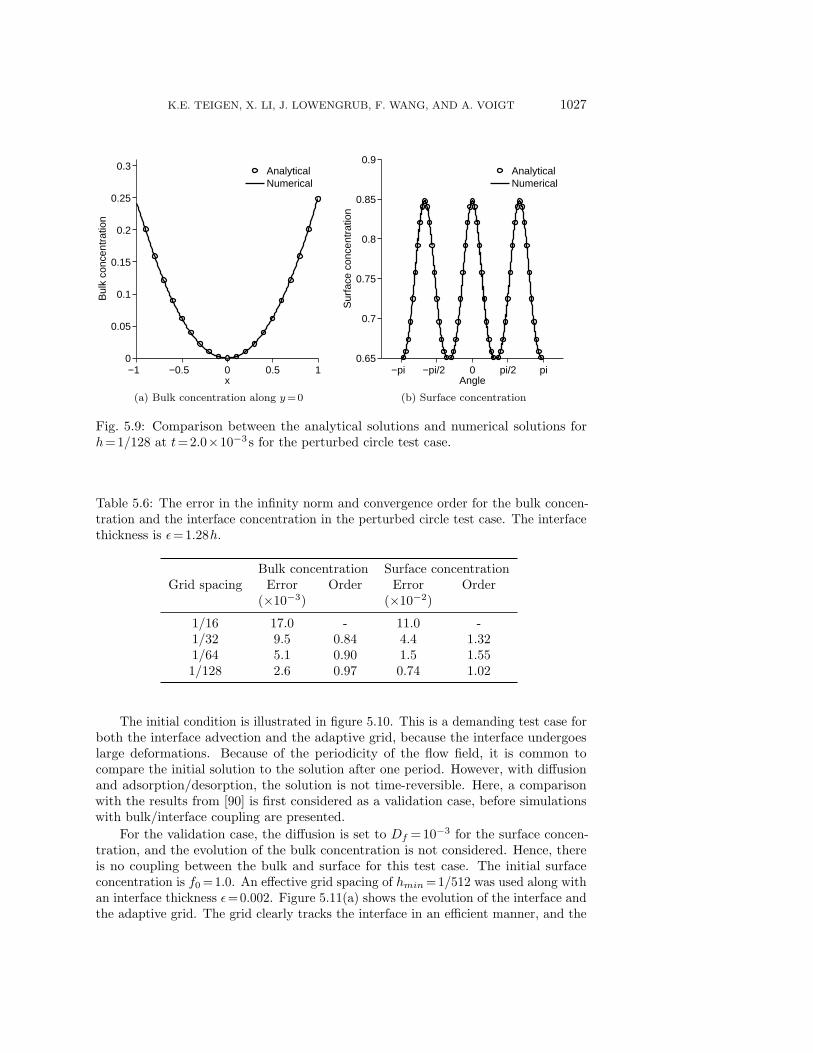
scaled as ε= 1.28hmin. Figure 5.8 shows the final solution for the surface concentrationand the bulk concentration for a grid spacing of hmin= 1/128. The analytical solutionsgiven by equations (5.17) and (5.18) are compared to the numerical results in figure 5.9.Excellent agreement is observed. In Table 5.6, the respective errors compared to theanalytical solutions are listed together with the convergence order. Again, first orderconvergence results are obtained.
5.6. Bulk-surface coupling in a 2D vortical flow A circle with radiusr= 0.15 is placed at x= (0.5,0.75) in a domain Ω = [0,1]× [0,1]. The circle is advectedby a prescribed velocity field defined by the stream function
Ψ =−cos(πt)1π
sin2(πx)sin2(πy), (5.22)
which gives the individual velocity components as
u=−2 cos(πt)sin2 (πx)sin(πy)cos(πy) , (5.23)
v= 2cos(πt) sin2 (πy)sin(πx)cos(πx). (5.24)
K.E. TEIGEN, X. LI, J. LOWENGRUB, F. WANG, AND A. VOIGT 1027
−1 −0.5 0 0.5 10
0.05
0.1
0.15
0.2
0.25
0.3
x
Bul
k co
ncen
trat
ion
AnalyticalNumerical
(a) Bulk concentration along y = 0
−pi −pi/2 0 pi/2 pi0.65
0.7
0.75
0.8
0.85
0.9
Angle
Sur
face
con
cent
ratio
n
AnalyticalNumerical
(b) Surface concentration
Fig. 5.9: Comparison between the analytical solutions and numerical solutions forh= 1/128 at t= 2.0×10⁻³ s for the perturbed circle test case.
Table 5.6: The error in the infinity norm and convergence order for the bulk concen-tration and the interface concentration in the perturbed circle test case. The interfacethickness is ε= 1.28h.
Bulk concentration Surface concentrationGrid spacing Error Order Error Order
(×10−3) (×10−2)
1/16 17.0 - 11.0 -1/32 9.5 0.84 4.4 1.321/64 5.1 0.90 1.5 1.551/128 2.6 0.97 0.74 1.02
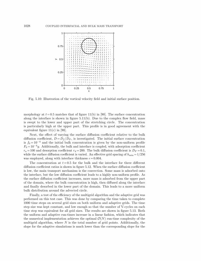
The initial condition is illustrated in figure 5.10. This is a demanding test case forboth the interface advection and the adaptive grid, because the interface undergoeslarge deformations. Because of the periodicity of the flow field, it is common tocompare the initial solution to the solution after one period. However, with diffusionand adsorption/desorption, the solution is not time-reversible. Here, a comparisonwith the results from [90] is first considered as a validation case, before simulationswith bulk/interface coupling are presented.
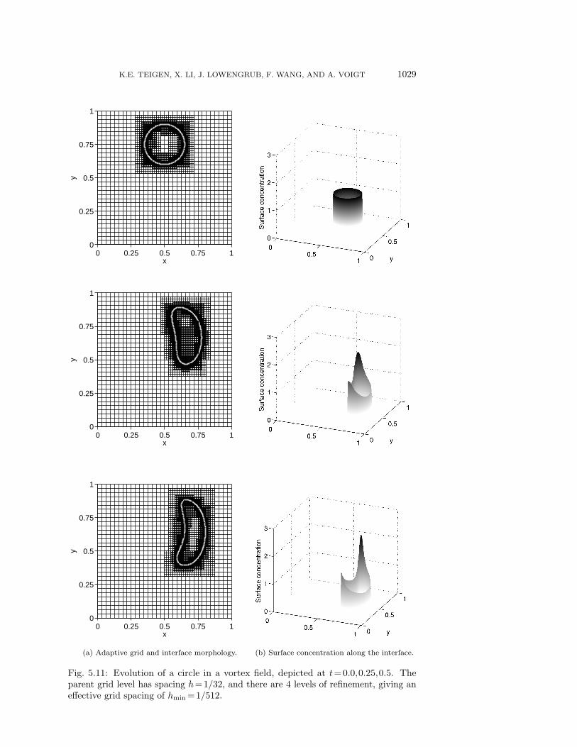
For the validation case, the diffusion is set to Df =10−3 for the surface concen-tration, and the evolution of the bulk concentration is not considered. Hence, thereis no coupling between the bulk and surface for this test case. The initial surfaceconcentration is f0 = 1.0. An effective grid spacing of hmin= 1/512 was used along withan interface thickness ε= 0.002. Figure 5.11(a) shows the evolution of the interface andthe adaptive grid. The grid clearly tracks the interface in an efficient manner, and the
1028 COUPLED INTERFACIAL AND BULK MASS TRANSPORT
x
y
0 0.25 0.5 0.75 10
0.25
0.5
0.75
1
Fig. 5.10: Illustration of the vortical velocity field and initial surface position.
morphology at t= 0.5 matches that of figure 11(b) in [90]. The surface concentrationalong the interface is shown in figure 5.11(b). Due to the complex flow field, massis swept to the lower and upper part of the stretching circle. The concentrationis particularly high at the upper part. This profile is in good agreement with theequivalent figure 11(c) in [90].
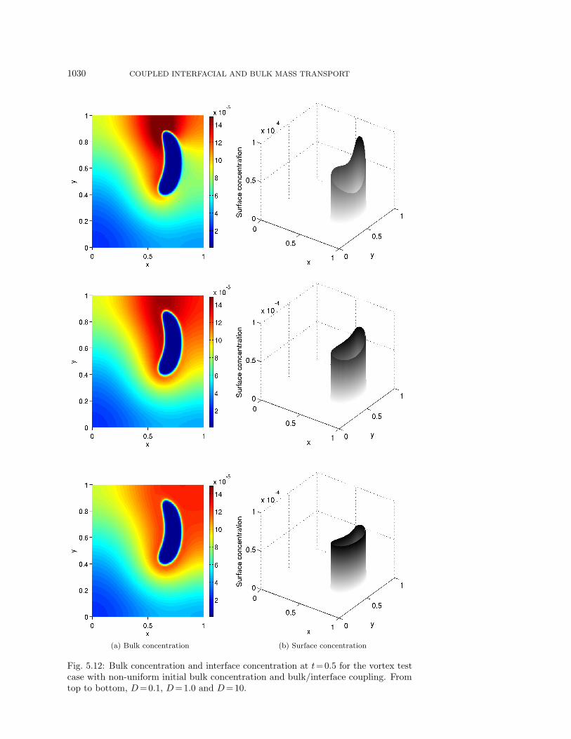
Next, the effect of varying the surface diffusion coefficient relative to the bulkdiffusion coefficient, D=Df/DF , is investigated. The initial surface concentrationis f0 =10−4 and the initial bulk concentration is given by the non-uniform profileF0 = 10−4y. Additionally, the bulk and interface is coupled, with adsorption coefficientra= 100 and desorption coefficient rd= 200. The bulk diffusion coefficient is DF = 0.1,while the surface diffusion coefficient is varied. An effective grid spacing of hmin = 1/256was employed, along with interface thickness ε= 0.004.
The concentration at t=0.5 for the bulk and the interface for three differentdiffusion coefficient ratios is shown in figure 5.12. When the surface diffusion coefficientis low, the main transport mechanism is the convection. Some mass is adsorbed ontothe interface, but the low diffusion coefficient leads to a highly non-uniform profile. Asthe surface diffusion coefficient increases, more mass is adsorbed from the upper partof the domain, where the bulk concentration is high, then diffused along the interfaceand finally desorbed in the lower part of the domain. This leads to a more uniformbulk distribution around the advected circle.
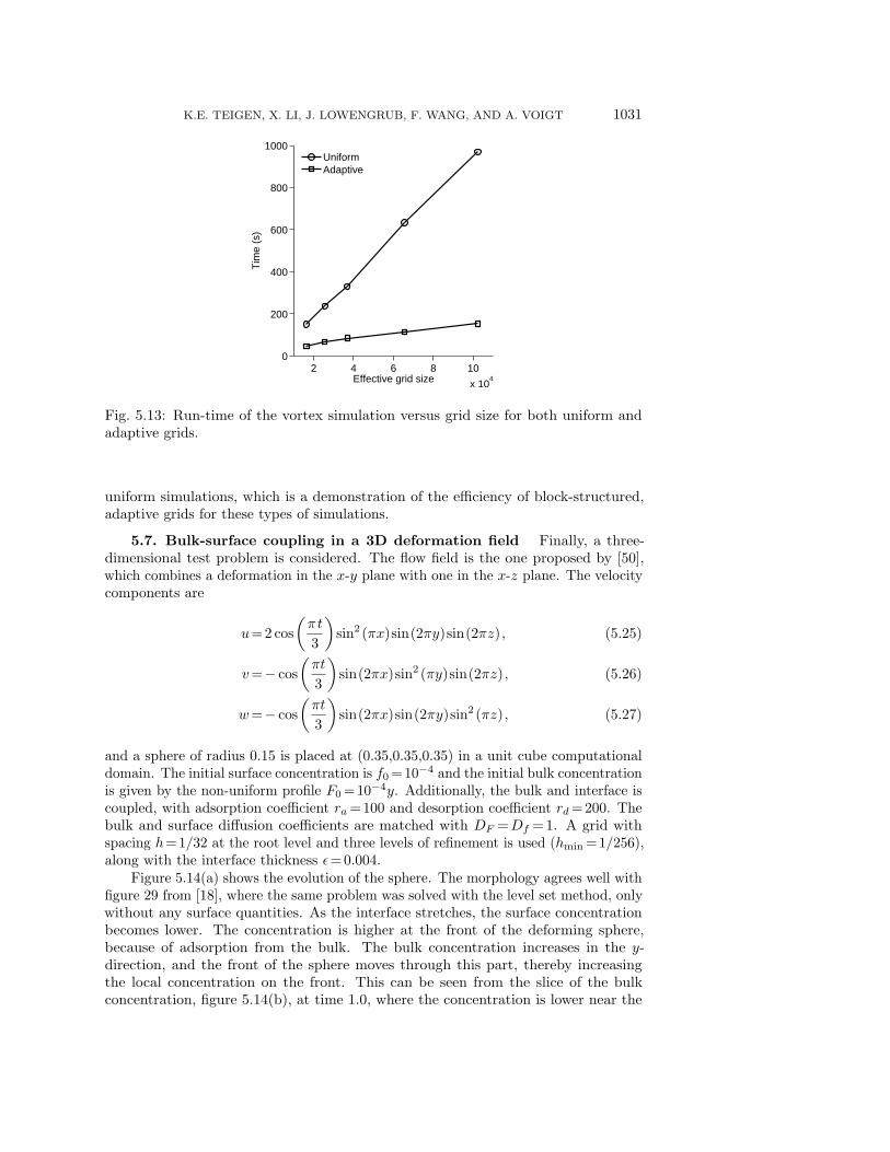
Finally, a test of the efficiency of the multigrid algorithm and the adaptive grid wasperformed on this test case. This was done by comparing the time taken to complete1000 time steps on several grid sizes on both uniform and adaptive grids. The timestep size was kept constant, and low enough so that the number of V-cycles on eachtime step was equivalent for all grid sizes. The results are shown in figure 5.13. Boththe uniform and adaptive run-times increase in a linear fashion, which indicates thatthe numerical implementation achieves the optimal O(N) run-time complexity of themultigrid algorithm, where N is the total number of grid points. Additionally, theslope for the adaptive simulations is much lower than the corresponding slope for the
K.E. TEIGEN, X. LI, J. LOWENGRUB, F. WANG, AND A. VOIGT 1029
0 0.25 0.5 0.75 10
0.25
0.5
0.75
1
x
y
0 0.25 0.5 0.75 10
0.25
0.5
0.75
1
x
y
0 0.25 0.5 0.75 10
0.25
0.5
0.75
1
x
y
(a) Adaptive grid and interface morphology. (b) Surface concentration along the interface.
Fig. 5.11: Evolution of a circle in a vortex field, depicted at t=0.0,0.25,0.5. Theparent grid level has spacing h= 1/32, and there are 4 levels of refinement, giving aneffective grid spacing of hmin = 1/512.
1030 COUPLED INTERFACIAL AND BULK MASS TRANSPORT
(a) Bulk concentration (b) Surface concentration
Fig. 5.12: Bulk concentration and interface concentration at t= 0.5 for the vortex testcase with non-uniform initial bulk concentration and bulk/interface coupling. Fromtop to bottom, D= 0.1, D= 1.0 and D= 10.
K.E. TEIGEN, X. LI, J. LOWENGRUB, F. WANG, AND A. VOIGT 1031
2 4 6 8 10
x 104
0
200
400
600
800
1000
Effective grid size
Tim
e (s
)
UniformAdaptive
Fig. 5.13: Run-time of the vortex simulation versus grid size for both uniform andadaptive grids.
uniform simulations, which is a demonstration of the efficiency of block-structured,adaptive grids for these types of simulations.
5.7. Bulk-surface coupling in a 3D deformation field Finally, a three-dimensional test problem is considered. The flow field is the one proposed by [50],which combines a deformation in the x-y plane with one in the x-z plane. The velocitycomponents are
u= 2 cos(πt
3
)sin2 (πx)sin(2πy)sin(2πz) , (5.25)
v=− cos(πt
3
)sin(2πx)sin2 (πy)sin(2πz) , (5.26)
w=− cos(πt
3
)sin(2πx)sin(2πy)sin2 (πz) , (5.27)
and a sphere of radius 0.15 is placed at (0.35,0.35,0.35) in a unit cube computationaldomain. The initial surface concentration is f0 = 10−4 and the initial bulk concentrationis given by the non-uniform profile F0 = 10−4y. Additionally, the bulk and interface iscoupled, with adsorption coefficient ra= 100 and desorption coefficient rd= 200. Thebulk and surface diffusion coefficients are matched with DF =Df =1. A grid withspacing h= 1/32 at the root level and three levels of refinement is used (hmin = 1/256),along with the interface thickness ε= 0.004.
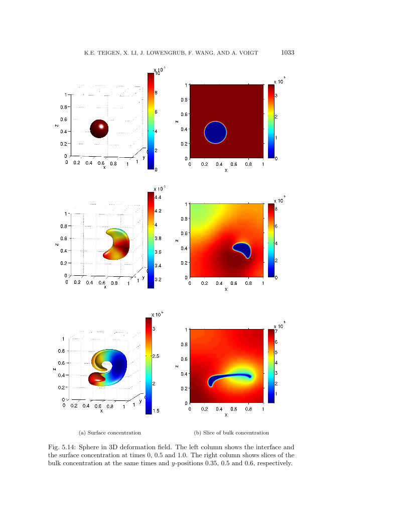
Figure 5.14(a) shows the evolution of the sphere. The morphology agrees well withfigure 29 from [18], where the same problem was solved with the level set method, onlywithout any surface quantities. As the interface stretches, the surface concentrationbecomes lower. The concentration is higher at the front of the deforming sphere,because of adsorption from the bulk. The bulk concentration increases in the y-direction, and the front of the sphere moves through this part, thereby increasingthe local concentration on the front. This can be seen from the slice of the bulkconcentration, figure 5.14(b), at time 1.0, where the concentration is lower near the
1032 COUPLED INTERFACIAL AND BULK MASS TRANSPORT
region that the interface has moved through. The middle of the stretched sphere has amuch lower concentration, due to the fact that it has experienced a large deformationand is in a region of low bulk concentration.
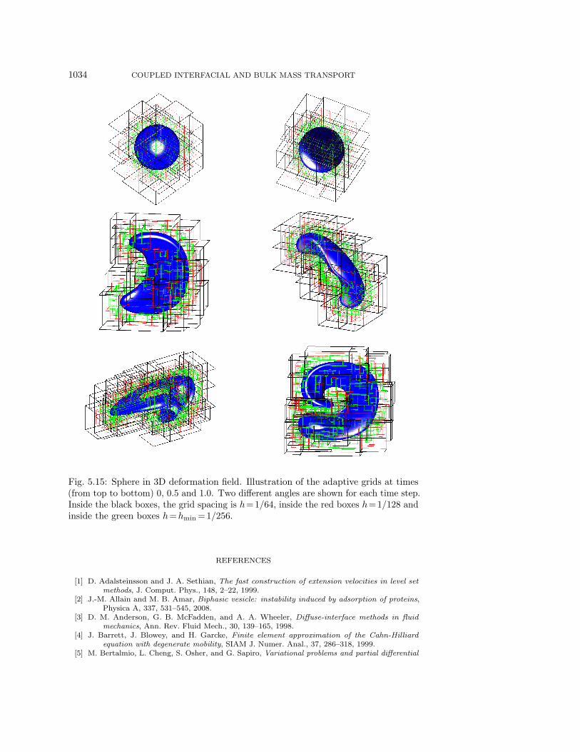
Figure 5.15 shows a sequence of the block-structured grids used in the simulation.The boxes denote grid level boundaries, so that inside each box the resolution isdoubled. This demonstrates that the adaptive grid algorithm also works well forthree-dimensional problems.
6. Conclusion A diffuse-interface method for solving problems involving trans-port, diffusion, and adsorption/desorption of a material quantity on a deformableinterface was presented. The method was shown to perform well on a wide range oftest cases. The efficiency of the numerical implementation, using adaptive grids and amultigrid method, was also demonstrated.
The asymptotic analysis suggests, and numerical evidence confirms, that theconvergence to the sharp interface system is first order in the interface thicknessparameter ε. It may be possible to gain second order accuracy in ε by explicitlyremoving the corresponding term in the asymptotic expansion as can be done in thecontext of solidification to enable simulations with arbitrary kinetic coefficients [43, 44].This should be explored.
A natural extension of the method is to couple it to an external flow solver.The ability of the diffuse-interface method to handle complex fluids and interfacialdynamics makes this a very attractive combination. We are currently developing suchan algorithm to simulate the dynamics of interfacial flows with soluble surfactants.Another interesting extension is to couple the method with models of cellular mechanicsto simulate cell-polarization and motility.
Finally, this work used a phase-field function to represent the interface. Alterna-tively, a level-set function could be used instead. Accurate representations of deltafunctions and Heaviside functions in the level-set context can be found in for example[80, 83, 68].
Acknowledgment. The authors thank Steven Wise and Fang Jin for assistancewith the numerical code and visualization, and the reviewers, whose comments haveimproved the paper. KET is funded by the project “Electrocoalescence – Criteria foran efficient process in real crude oil systems”; coordinated by SINTEF Energy Research.The project is supported by The Research Council of Norway, under the contract no:169466/S30, and by the following industrial partners: Aibel AS, Aker Solutions AS,BP Exploration Operating Company Ltd, Saudi Aramco, Shell Technology Norway AS,StatoilHydro ASA and Petrobras. KET also acknowledges support from the ResearchCouncil of Norway through grant IS-BILAT 192532 and from the Fulbright Foundation.FW, JL and XL acknowledge support from the National Science Foundation Divisionof Mathematical Sciences (DMS) and from the National Institutes of Health throughgrant P50GM76516 for a Centre of Excellence in Systems Biology at the University ofCalifornia, Irvine. AV acknowledges support from the German Science Foundationthrough grants Vo899/6-1 and SFB 609.
K.E. TEIGEN, X. LI, J. LOWENGRUB, F. WANG, AND A. VOIGT 1033
(a) Surface concentration (b) Slice of bulk concentration
Fig. 5.14: Sphere in 3D deformation field. The left column shows the interface andthe surface concentration at times 0, 0.5 and 1.0. The right column shows slices of thebulk concentration at the same times and y-positions 0.35, 0.5 and 0.6, respectively.
1034 COUPLED INTERFACIAL AND BULK MASS TRANSPORT
Fig. 5.15: Sphere in 3D deformation field. Illustration of the adaptive grids at times(from top to bottom) 0, 0.5 and 1.0. Two different angles are shown for each time step.Inside the black boxes, the grid spacing is h= 1/64, inside the red boxes h= 1/128 andinside the green boxes h=hmin = 1/256.
REFERENCES
[1] D. Adalsteinsson and J. A. Sethian, The fast construction of extension velocities in level setmethods, J. Comput. Phys., 148, 2–22, 1999.
[2] J.-M. Allain and M. B. Amar, Biphasic vesicle: instability induced by adsorption of proteins,Physica A, 337, 531–545, 2008.
[3] D. M. Anderson, G. B. McFadden, and A. A. Wheeler, Diffuse-interface methods in fluidmechanics, Ann. Rev. Fluid Mech., 30, 139–165, 1998.
[4] J. Barrett, J. Blowey, and H. Garcke, Finite element approximation of the Cahn-Hilliardequation with degenerate mobility, SIAM J. Numer. Anal., 37, 286–318, 1999.
[5] M. Bertalmio, L. Cheng, S. Osher, and G. Sapiro, Variational problems and partial differential
K.E. TEIGEN, X. LI, J. LOWENGRUB, F. WANG, AND A. VOIGT 1035
equations on implicit surfaces, J. Comput. Phys., 174, 759–780, 2001.[6] J. Blowey and C. Elliott, The Cahn-Hilliard gradient theory for phase separation with non-
smooth free energy part 1: mathematical analysis, Eur. J. Appl. Math., 2, 233–280, 1991.[7] J. Blowey and C. Elliott, The Cahn-Hilliard gradient theory for phase separation with non-
smooth free energy part 2: Numerical analysis, Eur. J. Appl. Math., 3, 147–179, 1992.[8] A. Bueno-Orovio and V. Perez-Garcia, Spectral methods for partial differential equations on
irregular domains: the spectral smoothed boundary method, SIAM J. Sci. Comput., 28,886–900, 2006.
[9] A. Bueno-Orovio and V. Perez-Garcia, Spectral smoothed boundary methods: the role of externalboundary conditions, Numer. Meth. Partial Diff. Eqns., 22, 435–448, 2006.
[10] G. Caginalp and P. Fife, Dynamics of layered interfaces arising from phase boundaries, SIAMJ. Appl. Math., 48, 506–518, 1988.
[11] P. Cermelli, E. Fried, and M. Gurtin, Transport relations for surface integrals arising in theformulation of balance laws for evolving fluid interfaces, J. Fluid Mech., 544, 339–351, 2005.
[12] C. Duarte, I. Babuska, and J. Oden, Generalized finite element methods for three-dimensionalstructural mechanics problems, Comp. Struct., 77, 215–232, 2000.
[13] G. Dziuk and C. Elliott, Eulerian finite element method for parabolic PDEs on complex surfaces,Int. Free Bound., 10, 119–138, 2008.
[14] G. Dziuk and C. Elliott, An Eulerian approach to transport and diffusion on evolving implicitsurfaces, Comput. Visualization Sci., in press, 2009.
[15] C. Eilks and C. Elliott, Numerical simulation of dealloying by surface dissolution by the evolvingsurface finite element method, J. Comput. Phys., 227, 9727–9741, 2008.
[16] C. Elliott and B. Stinner, Analysis of a diffuse interface approach to an advection diffusionequation on a moving surface, Math. Mod. Meth. Appl. Sci., in press, 2009.
[17] C. Elliott, B. Stinner, V. Styles, and R. Welford, Numerical computation of advection anddiffusion on evolving diffuse interfaces, preprint, 2009.
[18] D. Enright, R. Fedkiw, J. Ferziger, and I. Mitchell, A hybrid particle level set method forimproved interface capturing, J. Comput. Phys., 183, 83–116, 2002.
[19] J. Erlebacher, M. Aziz, A. Karma, N. Dimitrov, and K. Sieradzki, Evolution of nanoporosity indealloying, Nature, 410, 450–453, 2001.
[20] R. Fedkiw, T. Aslam, B. Merriman, and S. Osher, A non-oscillatory Eulerian approach tointerfaces in multimaterial flows (the ghost fluid method), J. Comput. Phys, 152, 457–492,1999.
[21] F. Fenton, E. Cherry, A. Karma, and W.-J. Rappel, Modeling wave propagation in realisticheart geometries using the phase-field method, Chaos, 15, 103502, 2005.
[22] P. Fife and O. Penrose, Interfacial dynamics for thermodynamically consistent phase-fieldmodels with nonconserved order parameter, Elect. J. Diff. Eqs., 16, 1–49, 1995.
[23] E. Fried and M. Gurtin, A unified treatment of evolving interfaces accounting for smalldeformations and atomic transport with emphasis on grain-boundaries and epitaxy, Adv.Appl. Mech., 40, 1–177, 2004.
[24] F. Gibou and R. Fedkiw, A fourth order accurate discretization for the Laplace and heatequations on arbitrary domains with applications to the Stefan problem, J. Comput. Phys,202, 577–601, 2005.
[25] F. Gibou, R. Fedkiw, L. Cheng, and M. Kang, A second order accurate symetric discretizationof the Poisson equation on irregular domains, J. Comput. Phys, 176, 205–227, 2002.
[26] J. Glimm, D. Marchesin, and O. McBryan, A numerical method for 2 phase flow with anunstable interface, J. Comput. Phys, 39, 179–200, 1981.
[27] R. Glowinski, T. Pan, and J. Periaux, A fictitious domain method for external incompressibleviscous-flow modeled by Navier-Stokes equations, Comput. Meth. Appl. Mech. Engin., 112,133–148, 1994.
[28] R. Glowinski, T. Pan, R. Wells, and X. Zhou, Wavelet and finite element solutions for theNeumann problem using fictitious domains, J. Comput. Phys., 126, 40–51, 1996.
[29] A. Gomez-Marin, J. Garcia-Ojalvo, and J. Sancho, Self-sustained spatiotemporal oscillationsinduced by membrane-bulk coupling, Phys. Rev. Lett., 98, 168303, 2007.
[30] J. Greer, A. Bertozzi, and G. Sapiro, Fourth order partial differential equations on generalgeometries, J. Comput. Phys., 216, 216–246, 2006.
[31] W. Hackbusch and S. Sauter, Composite finite elements for the approximation of PDEs ondomains with complicated micro-structures, Num. Math., 75, 447–472, 1997.
[32] M. Hameed, M. Siegel, Y.-N. Young, J. Li, M. R. Booty, and D. T. Papageorgiou, Influenceof insoluble surfactant on the deformation and breakup of a bubble or thread in a viscousfluid, J. of Fluid Mech., 594, 307–340, 2008.
[33] J. Hao, T. Pan, R. Glowinski, and D. Joseph, A fictitious domain/distributed lagrange multiplier
1036 COUPLED INTERFACIAL AND BULK MASS TRANSPORT
method for the particulate flow of Oldroyd-B fluids: a positive definiteness preservingapproach, J. Non-Newtonian Fluid Mech., 156, 95–111, 2009.
[34] A. Hirsa and W. W. Willmarth, Measurements of vortex pair interaction with a clean orcontaminated free surface, J. Fluid Mech., 259, 25–45, 1994.
[35] Y. T. Hu, D. J. Pine, and L. G. Leal, Drop deformation, breakup, and coalescence withcompatibilizer, Phys. Fluids, 12, 484–489, 2000.
[36] S. D. Hudson, A. M. Jamieson, and B. E. Burkhart, The effect of surfactant on the efficiencyof shear-induced drop coalescence, J. Colloid and Interface Science, 265, 409–421, 2003.
[37] K. Ito, M.-C. Lai, and Z. Li, A well-conditioned augmented system for solving Navier-Stokes inirregular domains, J. Comput. Phys., 228, 2616–2628, 2009.
[38] A. J. James and J. Lowengrub, A surfactant-conserving volume-of-fluid method for interfacialflows with insoluble surfactant, J. Comput. Phys., 201, 685–722, 2004.
[39] Y. J. Jan, Computational Studies of Bubble Dynamics, PhD thesis, University of Michigan,1994.
[40] H. Ji, F.-S. Lien, and E. Yee, An efficient second-order accurate cut-cell method for solvingthe variable coefficient Poisson equation with jump conditions on irregular domains, Int. J.Num. Meth. Fluids, 52, 723–748, 2006.
[41] H. Johansen and P. Colella, A Cartesian grid embedded boundary method for Poisson’s equationon irregular domains, J. Comput. Phys, 147, 60–85, 1998.
[42] H. Johansen and P. Colella, Embedded boundary algorithms and software for partial differentialequations, J. Phys., 125, 012084, 2008.
[43] A. Karma and W.-J. Rappel, Phase-field method for computationally efficient modeling ofsolidification with arbitrary interface kinetics, Phys. Rev. E, 53, R3017–R3020, 1996.
[44] A. Karma and W.-J. Rappel, Quantitative phase-field modeling of dendritic growth in two andthree dimensions, Phys. Rev. E, 57, 4323–4349, 1998.
[45] J.-S. Kim, K. Kang, and J. Lowengrub, Conservative multigrid methods for Cahn-Hilliard fluids,J. Comput. Phys., 193, 511–543, 2004.
[46] J. Kockelkoren, H. Levine, and W.-J. Rappel, Computational approach for modeling intra- andextracellular dynamics, Phys. Rev. E, 68, 037702, 2003.
[47] M.-C. Lai, Y.-H. Tseng, and H. Huang, An immersed boundary method for interfacial flowswith insoluble surfactant, J. Comput. Phys., 227, 7270–7293, 2008.
[48] L. G. Leal, Flow induced coalescence of drops in a viscous fluid, Phys. of Fluids, 16, 1833–1851,2004.
[49] R. LeVeque and Z. Li, The immersed interface method for elliptic equations with discontinuouscoefficients and singular sources, SIAM J. Num. Anal., 31, 1019–1044, 1997.
[50] R. J. Leveque, High-resolution conservative algorithms for advection in incompressible flow,SIAM J Numer. Anal., 33, 627–665, 1996.
[51] H. Levine and W.-J. Rappel, Membrane-bound Turing patterns, Phys. Rev. E, 72, 061912, 2005.[52] B. Li, J. Lowengrub, A. Ratz, and A. Voigt, Geometric evolution laws for thin crystalline films:
modeling and numerics, Commun. Comput. Phys., 6, 433–482, 2009.[53] X. Li, J. Lowengrub, A. Ratz, and A. Voigt, Solving PDEs in complex geometries: a diffuse
domain approach, Comm. Math. Sci., 7, 81–107, 2009.[54] Z. Li and K. Ito, The immersed interface method: Numerical solutions of PDEs involving
interfaces and irregular domains, SIAM Front. Appl. Math., 33, 2006.[55] S. Liu and T. Chan, Weighted essentially non-oscillatory schemes, J. Comput. Phys., 115,
200–212, 1994.[56] R. Lohner, J. Cebral, F. Camelli, J. Baum, E. Mestreau, and O. Soto, Adaptive embed-
ded/immersed unstructured grid techniques, Arch. Comput. Meth. Eng., 14, 279–301, 2007.[57] W. E. Lorensen and H. E. Cline, Marching cubes: a high resolution 3d surface construction
algorithm, Computer Graphics, 21, 163–169, 1987.[58] J. Lowengrub and L. Truskinovsky, Quasi-incompressible Cahn-Hilliard fluids and topological
transitions, R. Soc. Lond. Proc. Ser. A Math. Phys. Eng. Sci., 454, 2617–2654, 1998.[59] S. Lui, Spectral domain embedding for elliptic PDEs in complex domains, J. Comput. Appl.
Math., 225, 541–557, 2009.[60] P. Macklin and J. Lowengrub, Evolving interfaces via gradients of geometry-dependent interior
poisson problems: application to tumor growth, J. Comput. Phys, 203, 191–220, 2005.[61] P. Macklin and J. Lowengrub, A new ghost cell/level set method for moving boundary problems:
Application to tumor growth, J. Sci. Comput., 35, 266–299, 2008.[62] S. Marella, S. Krishnan, and H. Udaykumar, Sharp interface Cartesian grid method I: an easily
implemented technique for 3D moving boundary computations, J. Comput. Phys, 210, 1–31,2005.
[63] O. K. Matar and S. M. Troian, The development of transient fingering patterns during the
K.E. TEIGEN, X. LI, J. LOWENGRUB, F. WANG, AND A. VOIGT 1037
spreading of surfactant coated films, Phys. Fluids, 11, 3232–3246, 1999.[64] P. McCorquodale, P. Colella, and H. Johansen, A Cartesian grid embedded boundary method
for the heat equation on irregular domains, J. Comput. Phys, 173, 620–635, 2001.[65] J. Melenk and I. Babuska, The partition of unity finite element method: basic theory and
applications, Comp. Meth. Appl. Mech. Eng., 139, 289–314, 1996.[66] W. J. Milliken and L. G. Leal, The influence of surfactant on the deformation and breakup of a
viscous drop - the effect of surfactant solubility, J. Colloid and Interface Sci., 166, 275–285,1994.
[67] W. J. Milliken, H. A. Stone, and L. G. Leal, The effect of surfactant on transient motion ofNewtonian drops, Phys. Fluids A, 5, 69–79, 1993.
[68] C. Min and F. Gibou, Robust second-order accurate discretizations of the multi-dimensionalHeaviside and Dirac delta functions, J. Comput. Phys., 227, 9686–9695, 2008.
[69] M. Muradoglu and G. Tryggvason, A front-tracking method for computation of interfacial flowswith soluble surfactants, J. Comput. Phys., 227, 2238–2262, 2008.
[70] J. Oden, C. Duarte, and O. Zienkiewicz, A new cloud-based hp finite element method, Comp.Meth. Appl. Mech. Eng., 153, 117–126, 1998.
[71] R. Pego, Front migration in the nonlinear Cahn-Hilliard equation, Proc. Roy. Soc. London A,422, 261–278, 1989.
[72] I. Ramiere, P. Angot, and M. Belliard, A general fictitious domain method with immersed jumpsand multilevel nested structured meshes, J. Comput. Phys., 225, 1347–1387, 2007.
[73] A. Ratz and A. Voigt, PDEs on surfaces—a diffuse interface approach, Commun. Math. Sci., 4,575–590, 2006.
[74] M. Rech, S. Sauter, and A. Smolianski, Two-scale composite finite element method for Dirichletproblems on complicated domains, Num. Math., 102, 681–708, 2006.
[75] Y. Y. Renardy, M. Renardy, and V. Cristini, A new volume-of-fluid formulation for surfactantsand simulations of drop deformation under shear at a low viscosity ratio, European Journalof Mechanics - B/Fluids, 21, 49–59, 2002.
[76] P. Schwartz, M. Barad, P. Colella, and T. Ligocki, A Cartesian grid embedded boundary methodfor the heat equation and Poisson’s equation in three dimensions, J. Comput. Phys, 211,531–550, 2006.
[77] J. Sethian and Y. Shan, Solving partial differential equations on irregular domains with mov-ing interfaces, with applications to superconformal electrodeposition in semiconductormanufacturing, J. Comput. Phys, 227, 6411–6447, 2008.
[78] C. W. Shu and S. Osher, Efficient implementation of essentially non-oscillatory shock-capturingschemes, J. Comput. Phys., 77, 439–471, 1988.
[79] I. Singer-Loginova and H. Singer, The phase field technique for modeling multiphase materials,Rep. Prog. Phys., 71, 106501, 2008.
[80] P. Smereka, The numerical approximation of a delta function with application to level setmethods, J. Comput. Phys., 211, 77–90, 2006.
[81] C. Stocker and A. Voigt, A level set approach to anisotropic surface evolution with free adatoms,SIAM J. Appl. Math, 69, 64–80, 2008.
[82] H. A. Stone and L. G. Leal, The effect of surfactants on drop deformation and breakup, J. Fluid.Mech., 220, 161–186, 1990.
[83] J. D. Towers, Two methods for discretizing a delta function supported on a level set, J. Comput.Phys, 220, 915–931, 2007.
[84] S. M. Troian, E. Herbolzheimer, and S. A. Safran, Model for the fingering instability of spreadingsurfactant drops, Phys. Rev. Lett., 65, 333–336, 1990.
[85] U. Trottenberg, C. Oosterlee, and A. Schller, Multigrid, London, UK: Academic Press, 2000.[86] G. Tryggvason, J. Abdollahi-Alibeik, W. W. Willmarth, and A. Hirsa, Collision of a vortex
pair with a contaminated free surface, Phys. Fluids A, 4, 1215–1229, 1992.[87] S. Wise, J.-S. Kim, and J. Lowengrub, Solving the regularized, strongly anisotropic Cahn-Hilliard
equation by an adaptive nonlinear multigrid method, J. Comput. Phys., 226, 414–446, 2007.[88] J. J. Xu, Z. Li, J. Lowengrub, and H. Zhao, A level set method for interfacial flows with
surfactant, J. Comput. Phys, 212, 590–616, 2006.[89] J. J. Xu and H. Zhao, An Eulerian formulation for solving partial differential equations along a
moving interface, J. Sci. Comp., 19, 573–594, 2003.[90] X. Yang and A. J. James, An arbitrary Lagrangian-Eulerian (ALE) method for interfacial flows
with insoluble surfactants, FDMP, 3, 65–96, 2007.[91] J. Zhang, D. Eckmann, and P. Ayyaswamy, A front tracking method for a deformable intravas-
cular bubble in a tube with soluble surfactant transport, J. Comput. Phys., 214, 366–396,2006.