www.elsevier.com/locate/ynimg

NeuroImage 30 (2006) 88 – 101

Dynamic physiological modeling for functional diffuse

optical tomography

Solomon Gilbert Diamond,a,* Theodore J. Huppert,a Ville Kolehmainen,b

Maria Angela Franceschini,a Jari P. Kaipio,b Simon R. Arridge,c and David A. Boasa

aMassachusetts General Hospital, Athinoula A. Martinos Center for Biomedical Imaging, Charlestown, MA 02129, USAbDepartment of Applied Physics, University of Kuopio, PO Box 1627, 70211 Kuopio, FinlandcDepartment of Computer Science, University College London, Gower Street, London WC1E 6BT, UK

Received 1 August 2005; accepted 14 September 2005

Available online 20 October 2005

Diffuse optical tomography (DOT) is a noninvasive imaging technology

that is sensitive to local concentration changes in oxy- and deoxy-

hemoglobin. When applied to functional neuroimaging, DOT measures

hemodynamics in the scalp and brain that reflect competing metabolic

demands and cardiovascular dynamics. The diffuse nature of near-

infrared photon migration in tissue and the multitude of physiological

systems that affect hemodynamics motivate the use of anatomical and

physiological models to improve estimates of the functional hemody-

namic response. In this paper, we present a linear state-space model for

DOT analysis that models the physiological fluctuations present in the

data with either static or dynamic estimation. We demonstrate the

approach by using auxiliary measurements of blood pressure varia-

bility and heart rate variability as inputs to model the background

physiology in DOT data. We evaluate the improvements accorded by

modeling this physiology on ten human subjects with simulated

functional hemodynamic responses added to the baseline physiology.

Adding physiological modeling with a static estimator significantly

improved estimates of the simulated functional response, and further

significant improvements were achieved with a dynamic Kalman filter

estimator (paired t tests, n = 10, P < 0.05). These results suggest that

physiological modeling can improve DOT analysis. The further

improvement with the Kalman filter encourages continued research

into dynamic linear modeling of the physiology present in DOT.

Cardiovascular dynamics also affect the blood-oxygen-dependent

(BOLD) signal in functional magnetic resonance imaging (fMRI). This

state-space approach to DOT analysis could be extended to BOLD

fMRI analysis, multimodal studies and real-time analysis.

D 2005 Elsevier Inc. All rights reserved.

Keywords: Physiological modeling; State-space model; Near-infrared

spectroscopy; Diffuse optical tomography; Kalman filter; Time-series

analysis

1053-8119/$ - see front matter D 2005 Elsevier Inc. All rights reserved.

doi:10.1016/j.neuroimage.2005.09.016

* Corresponding author.

E-mail address: sdiamond@nmr.mgh.harvard.edu (S.G. Diamond).

Available online on ScienceDirect (www.sciencedirect.com).

Introduction

Diffuse optical tomography (DOT) is a noninvasive imaging

technology that uses near-infrared (IR) light to image biological

tissue. The dominant chromophores in this spectrum are oxy-

hemoglobin (HbO), deoxyhemoglobin (HbR), lipids and water.

The basis of DOT is in vivo dynamic near-infrared spectroscopy of

these dominant chromophores in the tissue. Tomographic images in

DOT are constructed by simultaneously measuring from many

regions that cover a larger volume of tissue. The achievable in-

plane resolution of DOT decreases rapidly with depth because

biological tissue is a highly scattering medium for near-infrared

light. This diffuse property of the light also limits the penetration

depth in the adult human brain imaging to about 3 cm, which is

sufficient to study most of the cerebral cortex. See Gibson et al.

(2005a) for a more complete description of DOT. Clinical and

research applications of DOT arise due to its specificity to the

physiologically relevant chromophores HbO and HbR. Potential

clinical and research applications for DOT abound in brain injury

(Vernieri et al., 1999; Chen et al., 2000; Nemoto et al., 2000;

Saitou et al., 2000), neurological diseases (Hock et al., 1996;

Fallgatter et al., 1997; Hanlon et al., 1999; Steinhoff et al., 1996;

Adelson et al., 1999; Sokol et al., 2000; Watanabe et al., 2000),

psychiatric disorders (Okada et al., 1996b; Eschweiler et al., 2000;

Matsuo et al., 2000; Okada et al., 1994; Fallgatter and Strik, 2000)

and in cognitive and behavioral neuroscience (Ruben et al., 1997;

Sakatani et al., 1999; Franceschini et al., 2003; Colier et al., 1999;

Sato et al., 1999). Other research areas for DOT include infant

monitoring (Chen et al., 2002; Hintz et al., 2001; Meek et al., 1999;

Baird et al., 2002; Pena et al., 2003; Taga et al., 2003) and breast

cancer detection (Jakubowski et al., 2004; Shah et al., 2004;

Dehghani et al., 2003; Srinivasan et al., 2003). DOT is particularly

suitable for in situ monitoring and multimodal imaging (Strangman

et al., 2002). The dynamics measured with DOT in the functional

neuroimaging application are caused by dynamics in blood volume

and oxygenation in the scalp and in the brain. The measured

S.G. Diamond et al. / NeuroImage 30 (2006) 88–101 89

hemodynamics are caused by systemic fluctuations associated with

cardiac pulsation, respiration, heart rate variations, vasomotion and

the vascular response to neuronal activity (Obrig et al., 2000;

Toronov et al., 2000).

The primary aim of DOT functional neuroimaging is to localize

and separate the stimulus-related brain function signal from the

background physiology. The main problems are that the back-

ground physiology is much stronger than the stimulus response and

that anatomical regions are mixed in the diffuse measurements. As

a result, the DOT inverse problem cannot be solved without some

prior knowledge about the relevant anatomy and physiology. Since

the nature of functional anatomy is that structure and function are

mutually informative, spatial and temporal prior knowledge should

be considered in concert. The challenge of DOT analysis is then to

design a framework that will accommodate spatiotemporal prior

knowledge in a numerically tractable inverse problem. We attempt

here to advance DOT analysis in this direction.

Biophysical modeling of near-infrared photon migration in

human tissue remains an active area of research. Although a

forward model of the relevant physics is captured by the radiative

transport equation (Chandrasekhar, 1960), its solution for the

complex geometry of the human head can only be approximated.

One approach is to apply a finite element numerical solution to the

diffusion approximation to the transport equation (Arridge, 1999).

Another approach is to use hybrid methods (Ripoll et al., 2001;

Hayashi et al., 2003). Others have used a Monte Carlo simulation

of the photon migration (Okada et al., 1996a; Fukui et al., 2003;

Boas et al., 2002). Optical absorption and scattering parameters for

different tissue types are still debated in the literature (Koyama et

al., 2005; Strangman et al., 2003). The spatial inverse problem is

highly ill posed and requires regularization. Both linear (Boas et

al., 2004b; Yamamoto et al., 2002; Hintz et al., 2001) and nonlinear

(Bluestone et al., 2001; Prince et al., 2003; Xu et al., 2005; Hebden

et al., 2004) reconstructions are commonly used in DOT.

Many physiological systems are involved in determining the

vascular, blood pressure and blood oxygen dynamics in the scalp

and brain during DOT functional neuroimaging experiments.

Models of the systemic cardiovascular system (Mukkamala and

Cohen, 2001) and cerebral autoregulation (Lu et al., 2004)

demonstrate how these complex systems interact to produce the

observed short-term physiological variability. Some of the key

factors are heart rate, stroke volume, arterial and venous

compliance. These cardiovascular parameters are mediated by

autonomic regulatory mechanisms such as the arterial and

cardiopulmonary baroreflexes and by cardiorespiratory coupling

in the medulla. Cerebral autoregulation maintains relatively

constant cerebral blood flow (CBF) irrespective of variations in

arterial blood pressure. Despite this autoregulation, short-term

variability in CBF is still present (Panerai, 2004). Local vaso-

motion is also present throughout the brain and introduces spatial

and temporal variability in hemodynamics (Mayhew et al., 1996).

Local cerebral vascular beds respond to the metabolic demands of

neurons with a localized increase in blood flow, which is called the

neurovascular response (Logothetis et al., 2001). Systemic blood

oxygen and cerebral hemodynamics are also affected by inspired

gas concentrations and ventilation rate (Rostrup et al., 2002).

One method to help separate out the background physiology in

neuroimaging data is to include noninvasive auxiliary physiolog-

ical measurements as inputs in the analysis. Many instruments can

be used during experiments to acquire these physiological

dynamics. Examples are the blood pressure monitor, pulse

oximeter, electrocardiogram (ECG), chest band respirometer,

spirometer and capnograph. Stationary linear regression methods

in fMRI analysis (Frackowiak et al., 2003) accept multiple

regressors that could easily include auxiliary physiological

measurements. Including these additional inputs is a small

extension of standard finite impulse response (FIR) deconvolution

techniques (Goutte et al., 2000), which make the assumption that

the FIR models are time invariant. Zwiener et al. (2001)

investigated short-term coordinations between respiratory move-

ments, heart rate fluctuations and arterial blood pressure fluctua-

tions with partial coherence analysis. They concluded that there are

direct and changing coordinations between all three parameters to

different extents within the respiratory frequency range even

during paced breathing. These changing coordinations suggest

that the physiological effects are non-stationary and that dynamic

analysis methods may be more appropriate.

Dynamical methods in fMRI analysis have been applied with

parametric models of the functional response and a wide variety of

statistical methods (Gossl et al., 2000; Riera et al., 2004; Friston,

2002). These methods from fMRI are not directly transferable to

DOT because of differences in the biophysical models and relative

spatial and temporal resolution. In the DOT literature, Kolehmai-

nen et al. (2003) applied dynamic state-space estimation without

physiological regressors. Prince et al. (2003) fit the amplitude and

phase angle of three non-stationary sinusoids to DOT time-series

data using the Kalman filter. The three sinusoids were intended to

model the cardiac pulsations, respiratory affects and functional

response to a blocked experimental design. While supporting the

principle of using the dynamic Kalman filter in DOT analysis, the

three-sinusoid model does not allow for the most commonly used

event-related experimental designs nor can it use readily available

physiological measurements such as blood pressure as a regressor.

Zhang et al. (2005b) used principal component analysis (PCA) to

reduce the background physiological variance in functional

neuroimaging experiments. Anecdotal evidence was presented that

certain principal components correlate with blood pressure and

respiratory dynamics, but, since PCA analysis does not accept

exogenous inputs, any additional information contained in the

physiological measurements is not actually used. Known respira-

tory interactions in blood pressure regulation (Cohen and Taylor,

2002) suggest that the orthogonal projections in PCA are likely to

be mixtures of physiological effects. Due to the blind nature of

PCA, it is unclear how the principal components relate to prior

information from anatomical and physiological models.

In this paper, we present a state-space model that incorporates

most of the relevant anatomy, physiology and physics for DOT.

Unknown parameters in the proposed model can then be estimated

with the static and dynamic methods that we discuss. We evaluate

the model on data from ten human subjects with simulated local

hemodynamic responses added to the baseline physiology. With

this evaluation method, we confirm that the simulated activations

can be recovered and compare the results with and without

physiological inputs and from static and dynamic estimators.

A state-space model for DOT

We illustrate the anatomy, physiology and physics related to

DOT in the schematic of Fig. 1a with a level of complexity that is

intended to facilitate the design of a state-space analog. Within the

model, an experimental design determines the timing of events to

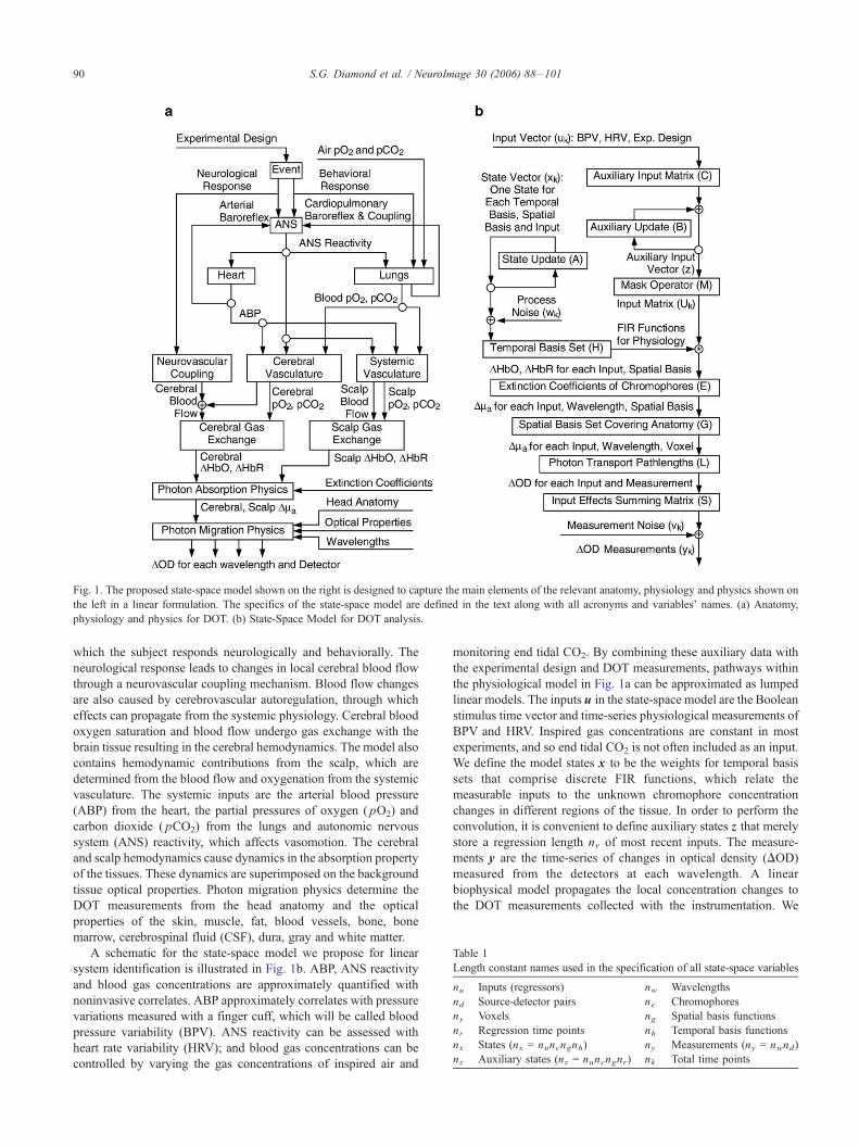
Fig. 1. The proposed state-space model shown on the right is designed to capture the main elements of the relevant anatomy, physiology and physics shown on

the left in a linear formulation. The specifics of the state-space model are defined in the text along with all acronyms and variables’ names. (a) Anatomy,

physiology and physics for DOT. (b) State-Space Model for DOT analysis.

Table 1

Length constant names used in the specification of all state-space variables

nu Inputs (regressors) nw Wavelengths

nd Source-detector pairs nc Chromophores

ns Voxels ng Spatial basis functions

nr Regression time points nh Temporal basis functions

nx States (nx = nuncngnh) ny Measurements (ny = nwnd)

nz Auxiliary states (nz = nuncngnr) nk Total time points

S.G. Diamond et al. / NeuroImage 30 (2006) 88–10190

which the subject responds neurologically and behaviorally. The

neurological response leads to changes in local cerebral blood flow

through a neurovascular coupling mechanism. Blood flow changes

are also caused by cerebrovascular autoregulation, through which

effects can propagate from the systemic physiology. Cerebral blood

oxygen saturation and blood flow undergo gas exchange with the

brain tissue resulting in the cerebral hemodynamics. The model also

contains hemodynamic contributions from the scalp, which are

determined from the blood flow and oxygenation from the systemic

vasculature. The systemic inputs are the arterial blood pressure

(ABP) from the heart, the partial pressures of oxygen ( pO2) and

carbon dioxide ( pCO2) from the lungs and autonomic nervous

system (ANS) reactivity, which affects vasomotion. The cerebral

and scalp hemodynamics cause dynamics in the absorption property

of the tissues. These dynamics are superimposed on the background

tissue optical properties. Photon migration physics determine the

DOT measurements from the head anatomy and the optical

properties of the skin, muscle, fat, blood vessels, bone, bone

marrow, cerebrospinal fluid (CSF), dura, gray and white matter.

A schematic for the state-space model we propose for linear

system identification is illustrated in Fig. 1b. ABP, ANS reactivity

and blood gas concentrations are approximately quantified with

noninvasive correlates. ABP approximately correlates with pressure

variations measured with a finger cuff, which will be called blood

pressure variability (BPV). ANS reactivity can be assessed with

heart rate variability (HRV); and blood gas concentrations can be

controlled by varying the gas concentrations of inspired air and

monitoring end tidal CO2. By combining these auxiliary data with

the experimental design and DOT measurements, pathways within

the physiological model in Fig. 1a can be approximated as lumped

linear models. The inputs u in the state-space model are the Boolean

stimulus time vector and time-series physiological measurements of

BPV and HRV. Inspired gas concentrations are constant in most

experiments, and so end tidal CO2 is not often included as an input.

We define the model states x to be the weights for temporal basis

sets that comprise discrete FIR functions, which relate the

measurable inputs to the unknown chromophore concentration

changes in different regions of the tissue. In order to perform the

convolution, it is convenient to define auxiliary states z that merely

store a regression length nr of most recent inputs. The measure-

ments y are the time-series of changes in optical density (DOD)

measured from the detectors at each wavelength. A linear

biophysical model propagates the local concentration changes to

the DOT measurements collected with the instrumentation. We

Table 2

State-space variable names

k Time index u(nu ,1)(k) Input vector

x(nx ,1)(k) State vector V(nx,nx)

(k) State covariance

w(nx ,1)(k) Process noise Q(nx,nx)

Process noise covariance

z(nz ,1)(k) Auxiliary state vector y (ny,1)

(k) Measurement vector

v(ny,1)(k) Measurement noise R(ny,ny)

Measurement noise covariance

A(nx ,nx)State update model B(nz ,nz)

Auxiliary update model

C(nz ,nu)Auxiliary input model D(ny,nx)

(k) Measurement model

K(nx ,ny)(k) Kalman gain matrix S(ny,nuny)

Summing matrix

U(nuncng ,nz)(k) Input matrix M(nuncng ,nz)

Input mask matrix

L(nuny,nunwns)Pathlength matrix L0(ny,nwns)

Pathlength submatrix

G(nunwns ,nunwng)Spatial basis set G0(ns ,ng)

Spatial submatrix

E(nunwng ,nuncng)Extinction matrix E0(nw,nc)

Extinction submatrix

H(nz ,nx)Temporal basis set H0(nr,nh)

Temporal submatrix

The respective sizes of each variable are indicated with parenthetical subscript notation and those that vary with the time index are indicated.

S.G. Diamond et al. / NeuroImage 30 (2006) 88–101 91

define all the constants and variables for the state-space model in

Tables 1 and 2 and further explain the model elements subsequently.

Our state-space model shown in Fig. 1b is a discrete-time

process that we will now describe in detail. In the following

description, we will use the notations T for the transpose operator,‘for the Kronecker tensor product, R for term-by-term array multi-

plication, I for the identity matrix, 1 for a matrix of ones, 0 for a

matrix of zeros, and matrix sizes will be indicated with parenthetical

subscripts.

Starting with the input vector u, the auxiliary state update

described by Eq. (1) buffers the input vector u into an auxiliary

state vector z storing nr time points of each input. The auxiliary

input model C places the current time step of the input vector u

into its proper location in the auxiliary state vector z. The auxiliary

update model B has a structure that advances the buffered inputs in

z by one time step

zk ¼ Bzk � 1 þ Cuk ; ð1Þ

C ¼ I nuð Þ ‘ 1ðncng ;1Þ‘1ð1; 1Þ0 nr � 1;1ð Þ

��; ð2Þ

B ¼ IðnuncngÞ ‘0 1;nr � 1ð Þ 0ð1; 1ÞI nr � 1ð Þ 0 nr � 1;1ð Þ

��: ð3Þ

The mask matrix M is used to arrange the auxiliary states into

an input matrix U that allows multiple convolutions with the inputs

to be performed with a single matrix multiplication

M ¼ IðnuncngÞ ‘ 1 1;nrð Þ; ð4Þ

Uk ¼ 1ðnuncng ;1ÞzTk RM: ð5Þ

The state vector x in Fig. 1b contains the weights for the

temporal basis set H that comprises the finite impulse response

functions used to model the physiology related to each input. The

state update defined by Eq. (6) is a first order autoregressive model

for the temporal evolution of the state vector x. We have defined the

state update model A as an identity, which specifies no inherent

growth or decay of the states. The process noise w is added at each

time step

xk ¼ Axk � 1 þ wk ð6Þ

A ¼ I nxð Þ: ð7Þ

The measurement update of Eq. (8) effectively filters the inputs

u with order nr � 1 finite impulse response filters defined by the

states x to predict the dynamics in the measurements y. The

measurement noise v adds to the measurement vector y at each

time step. The elements of the measurement model D are contained

in Eq. (9) and are also shown in Fig. 1b

yk ¼ D Ukð Þxk þ vk ; ð8Þ

D Ukð Þ ¼ SLGEUkH: ð9ÞThe states x operate through temporal H and spatial G basis

sets, which have the Kronecker product structure

H ¼ IðnuncngÞ ‘H0; ð10Þ

G ¼ IðnunwÞ ‘G0: ð11Þ

The columns of the temporal submatrix H0 contain temporal

basis functions to reduce the number of states and/or impose

temporal smoothing. The columns of the spatial submatrix G0

contain a set of spatial basis functions that can be used to reduce

the number of states and/or impose spatial smoothing of the state

estimates.

The optical extinction coefficients for the chromophores present

in the tissue volume are contained in the wavelength by

chromophore submatrix E0 and then copied and arranged into

the extinction matrix E. The pathlength submatrix L0 is a block

diagonal matrix formed from detector by voxel average effective

pathlengths for each wavelength as described by Arridge et al.

(1992). The pathlength matrix L captures the relevant physics for

linear tomographic reconstructions for the set of continuous wave

measurements in y

E ¼ I nuð Þ ‘E0 ‘ IðngÞ; ð12Þ

L ¼ I nuð Þ ‘L0: ð13Þ

The last element of the state-space model is a summing matrix S,

which combines the effects of multiple inputs in u into the

measurements y

Sk ¼ 1ð1;nuÞ ‘ IðnyÞ: ð14Þ

Static least-squares estimator

For the static least-squares estimator, we first pre-calculate Uk

and D(Uk) for all time steps k and then arrange the forward model

ys ¼ Dsx; ð15Þ

S.G. Diamond et al. / NeuroImage 30 (2006) 88–10192

where ys is the concatenation of yk at every time step

ys ¼ y 1½ �Ty 2½ �T . . . y nk½ �Tih T

; ð16Þ

and Ds is a similar concatenation of Dk

Ds ¼ D 1½ �TD 2½ �T>D nk½ �Tih T

: ð17Þ

We then use a standard Tikhonov or ridge regression estimator

for x

xx DTs Ds þ a2I nxð Þ

� ��1DT

s ys; ð18Þ

where a is the regularization parameter. There are many other

linear estimators that could be used in place of Eq. (18). Kay

(1993) discusses most of the common alternatives. We chose to

use Tikhonov here because of its simplicity and wide general

use.

Dynamic Kalman filter estimator

The Kalman filter is a recursive solution to discrete linear

filtering and prediction problems such as our proposed state-space

model (Kalman, 1960). The objective of the Kalman filter is to

obtain the best state estimates xk)k � 1 in a mean square sense

given all the data up to that time {y1,. . .,yk}. There are many

ways to model the same physical system within the generality of

the Kalman filter, and so the following discussion is limited to

our proposed model. The Kalman filter recursions require

initialization of the state vector estimate x0 and estimated state

covariance V0. Statistical covariance priors must also be specified

for the state process noise cov(w) = Q and the measurement noise

cov(v) = R. The algorithm can then proceed with the following

prediction-correction recursion.

First, the auxiliary state vector z and measurement model D are

updated

zk kk � 1 ¼ Bzk � 1kk � 1 þ Cuk ; ð19Þ

Uk ¼ 1ðnuncng ;1ÞzTk kk � 1 RM; ð20Þ

Dk ¼ SLGEUkH: ð21ÞNext the state vector x and state covariance V are predicted

xxk kk � 1 ¼ Axxk � 1kk � 1; ð22Þ

VVk kk � 1 ¼ AVVk � 1kk � 1AT þQ: ð23Þ

The Kalman gain matrix K is then computed

Kk ¼ VVk kk � 1DTk DkVVk kk � 1D

Tk þ R

� ��1; ð24Þ

and the auxiliary state vector z, state vector x and state covariance

V predictions are corrected with the new measurements y that are

available at time step k

zk kk ¼ zk kk � 1; ð25Þ

xxk kk ¼ xxk kk � 1 þKt yk � Dk xxk kk � 1

� �; ð26Þ

VVk kk ¼ VVk kk � 1 � KkDkVVk kk� 1: ð27Þ

Model validation

The salient feature of the state-space model we propose for

DOT analysis is physiological modeling. We designed the

following experiment to validate that the model reduces physio-

logical interference in estimates of a functional hemodynamic

response. The approach we took was to add a simulated functional

response to real data and then attempt to recover the simulated

response. Adding a simulated response allowed us to quantitatively

evaluate the analysis methods by comparing the estimated

responses with the ‘‘true’’ response that could not be directly

measured otherwise. We hypothesized that including blood

pressure variability and heart rate variability as inputs u would

model some of the real physiological variance and thereby improve

estimates of the simulated response. We also hypothesized that

allowing dynamic estimation of the physiological models would

further improve the simulated response estimates.

Baseline DOT data were collected approximately over the right

sensorimotor area of ten human subjects (9 male, 1 female, median

age 31, 9 right hand dominant, 1 left hand dominant). The subjects

were instructed to lie quietly in the dark and to breathe freely. The

raw optical measurements were collected with a continuous wave

DOT instrument (Franceschini et al., 2003), demodulated and

down sampled to 1 Hz. The photon fluence and auxiliary

physiological measurements were high-pass-filtered in a forward

then reverse direction with a 6th order IIR Butterworth filter with a

cutoff frequency of 0.05 Hz and zero phase distortion. This

filtering step removes slow physiology that is sufficiently outside

the frequency range of interest for the hemodynamic response that

it can be ignored. Short-term physiological variability including the

respiratory sinus arrhythmia, Mayer waves and vasomotion is still

present after filtering. The photon fluence U(t, k) was then

converted to a change in optical density DOD

DOD t; kð Þ ¼ lnU t; kð ÞU0 kð Þ

��; ð28Þ

where U0 was the average detected photon fluence and DOD(t, k)are the measurements y for the state-space model. The three model

inputs contained in u were the Boolean stimulus time vector, the

blood pressure variability (BPV) and heart rate variability (HRV)

with normalized variances.

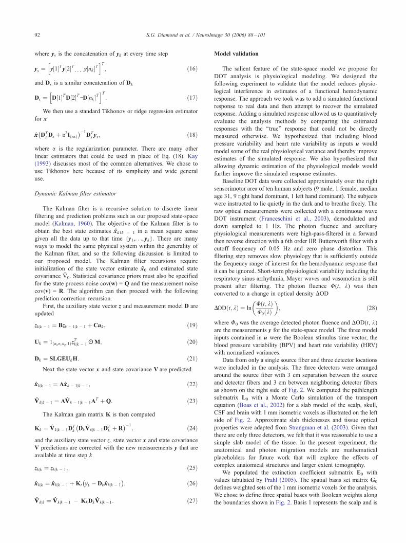
Data from only a single source fiber and three detector locations

were included in the analysis. The three detectors were arranged

around the source fiber with 3 cm separation between the source

and detector fibers and 3 cm between neighboring detector fibers

as shown on the right side of Fig. 2. We computed the pathlength

submatrix L0 with a Monte Carlo simulation of the transport

equation (Boas et al., 2002) for a slab model of the scalp, skull,

CSF and brain with 1 mm isometric voxels as illustrated on the left

side of Fig. 2. Approximate slab thicknesses and tissue optical

properties were adapted from Strangman et al. (2003). Given that

there are only three detectors, we felt that it was reasonable to use a

simple slab model of the tissue. In the present experiment, the

anatomical and photon migration models are mathematical

placeholders for future work that will explore the effects of

complex anatomical structures and larger extent tomography.

We populated the extinction coefficient submatrix E0 with

values tabulated by Prahl (2005). The spatial basis set matrix G0

defines weighted sets of the 1 mm isometric voxels for the analysis.

We chose to define three spatial bases with Boolean weights along

the boundaries shown in Fig. 2. Basis 1 represents the scalp and is

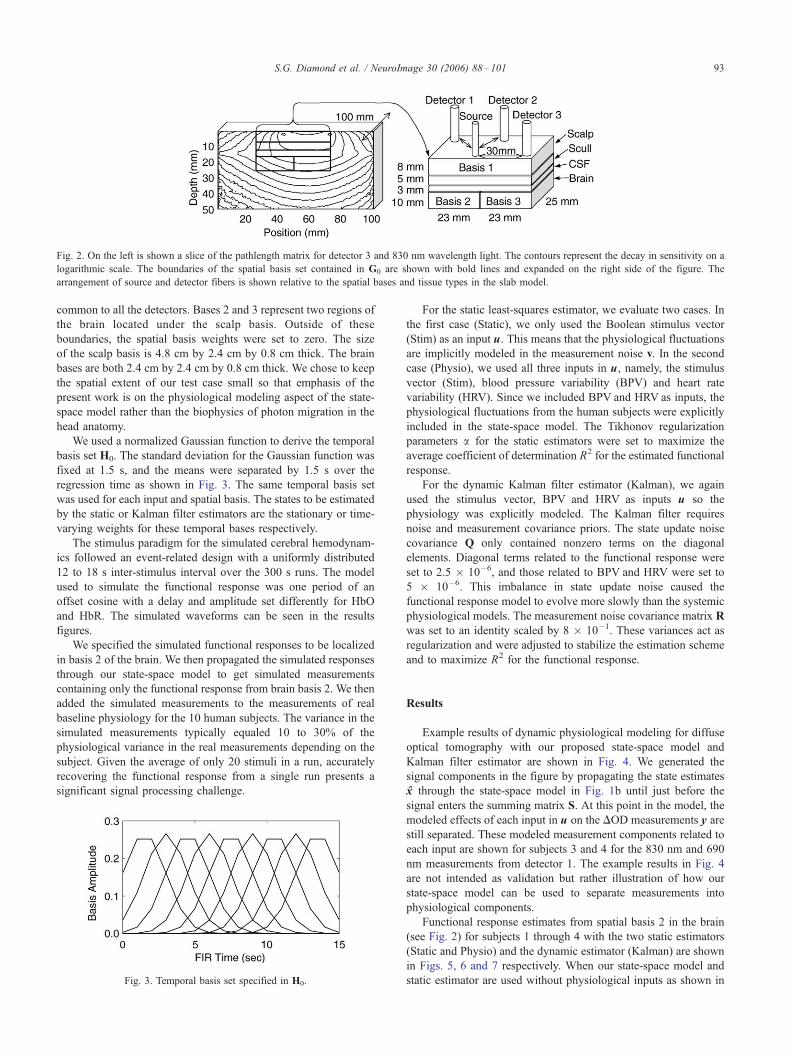
Fig. 2. On the left is shown a slice of the pathlength matrix for detector 3 and 830 nm wavelength light. The contours represent the decay in sensitivity on a

logarithmic scale. The boundaries of the spatial basis set contained in G0 are shown with bold lines and expanded on the right side of the figure. The

arrangement of source and detector fibers is shown relative to the spatial bases and tissue types in the slab model.

S.G. Diamond et al. / NeuroImage 30 (2006) 88–101 93

common to all the detectors. Bases 2 and 3 represent two regions of

the brain located under the scalp basis. Outside of these

boundaries, the spatial basis weights were set to zero. The size

of the scalp basis is 4.8 cm by 2.4 cm by 0.8 cm thick. The brain

bases are both 2.4 cm by 2.4 cm by 0.8 cm thick. We chose to keep

the spatial extent of our test case small so that emphasis of the

present work is on the physiological modeling aspect of the state-

space model rather than the biophysics of photon migration in the

head anatomy.

We used a normalized Gaussian function to derive the temporal

basis set H0. The standard deviation for the Gaussian function was

fixed at 1.5 s, and the means were separated by 1.5 s over the

regression time as shown in Fig. 3. The same temporal basis set

was used for each input and spatial basis. The states to be estimated

by the static or Kalman filter estimators are the stationary or time-

varying weights for these temporal bases respectively.

The stimulus paradigm for the simulated cerebral hemodynam-

ics followed an event-related design with a uniformly distributed

12 to 18 s inter-stimulus interval over the 300 s runs. The model

used to simulate the functional response was one period of an

offset cosine with a delay and amplitude set differently for HbO

and HbR. The simulated waveforms can be seen in the results

figures.

We specified the simulated functional responses to be localized

in basis 2 of the brain. We then propagated the simulated responses

through our state-space model to get simulated measurements

containing only the functional response from brain basis 2. We then

added the simulated measurements to the measurements of real

baseline physiology for the 10 human subjects. The variance in the

simulated measurements typically equaled 10 to 30% of the

physiological variance in the real measurements depending on the

subject. Given the average of only 20 stimuli in a run, accurately

recovering the functional response from a single run presents a

significant signal processing challenge.

Fig. 3. Temporal basis set specified in H0.

For the static least-squares estimator, we evaluate two cases. In

the first case (Static), we only used the Boolean stimulus vector

(Stim) as an input u. This means that the physiological fluctuations

are implicitly modeled in the measurement noise v. In the second

case (Physio), we used all three inputs in u, namely, the stimulus

vector (Stim), blood pressure variability (BPV) and heart rate

variability (HRV). Since we included BPV and HRV as inputs, the

physiological fluctuations from the human subjects were explicitly

included in the state-space model. The Tikhonov regularization

parameters a for the static estimators were set to maximize the

average coefficient of determination R2 for the estimated functional

response.

For the dynamic Kalman filter estimator (Kalman), we again

used the stimulus vector, BPV and HRV as inputs u so the

physiology was explicitly modeled. The Kalman filter requires

noise and measurement covariance priors. The state update noise

covariance Q only contained nonzero terms on the diagonal

elements. Diagonal terms related to the functional response were

set to 2.5 � 10�6, and those related to BPV and HRV were set to

5 � 10�6. This imbalance in state update noise caused the

functional response model to evolve more slowly than the systemic

physiological models. The measurement noise covariance matrix R

was set to an identity scaled by 8 � 10�1. These variances act as

regularization and were adjusted to stabilize the estimation scheme

and to maximize R2 for the functional response.

Results

Example results of dynamic physiological modeling for diffuse

optical tomography with our proposed state-space model and

Kalman filter estimator are shown in Fig. 4. We generated the

signal components in the figure by propagating the state estimates

x through the state-space model in Fig. 1b until just before the

signal enters the summing matrix S. At this point in the model, the

modeled effects of each input in u on the DOD measurements y are

still separated. These modeled measurement components related to

each input are shown for subjects 3 and 4 for the 830 nm and 690

nm measurements from detector 1. The example results in Fig. 4

are not intended as validation but rather illustration of how our

state-space model can be used to separate measurements into

physiological components.

Functional response estimates from spatial basis 2 in the brain

(see Fig. 2) for subjects 1 through 4 with the two static estimators

(Static and Physio) and the dynamic estimator (Kalman) are shown

in Figs. 5, 6 and 7 respectively. When our state-space model and

static estimator are used without physiological inputs as shown in

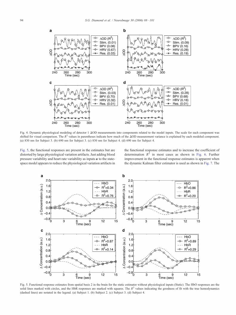
Fig. 4. Dynamic physiological modeling of detector 1 DOD measurements into components related to the model inputs. The scale for each component was

shifted for visual comparison. The R2 values in parentheses indicate how much of the DOD measurement variance is explained by each modeled component.

(a) 830 nm for Subject 3. (b) 690 nm for Subject 3. (c) 830 nm for Subject 4. (d) 690 nm for Subject 4.

S.G. Diamond et al. / NeuroImage 30 (2006) 88–10194

Fig. 5, the functional responses are present in the estimates but are

distorted by large physiological variation artifacts. Just adding blood

pressure variability and heart rate variability as inputs u to the state-

spacemodel appears to reduce the physiological variation artifacts in

Fig. 5. Functional response estimates from spatial basis 2 in the brain for the static

solid lines marked with circles, and the HbR responses are marked with squares.

(dashed lines) are notated in the legend. (a) Subject 1. (b) Subject 2. (c) Subject

the functional response estimates and to increase the coefficient of

determination R2 in most cases as shown in Fig. 6. Further

improvement in the functional response estimates is apparent when

the dynamic Kalman filter estimator is used as shown in Fig. 7. The

estimator without physiological inputs (Static). The HbO responses are the

The R2 values indicating the goodness of fit with the true hemodynamics

3. (d) Subject 4.

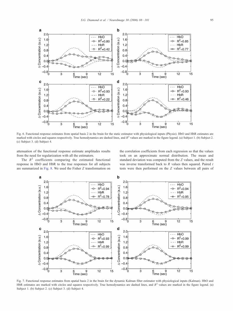
Fig. 6. Functional response estimates from spatial basis 2 in the brain for the static estimator with physiological inputs (Physio). HbO and HbR estimates are

marked with circles and squares respectively. True hemodynamics are dashed lines, and R2 values are marked in the figure legend. (a) Subject 1. (b) Subject 2.

(c) Subject 3. (d) Subject 4.

S.G. Diamond et al. / NeuroImage 30 (2006) 88–101 95

attenuation of the functional response estimate amplitudes results

from the need for regularization with all the estimators.

The R2 coefficients comparing the estimated functional

response in HbO and HbR to the true responses for all subjects

are summarized in Fig. 8. We used the Fisher Z transformation on

Fig. 7. Functional response estimates from spatial basis 2 in the brain for the dyn

HbR estimates are marked with circles and squares respectively. True hemodyna

Subject 1. (b) Subject 2. (c) Subject 3. (d) Subject 4.

the correlation coefficients from each regression so that the values

took on an approximate normal distribution. The mean and

standard deviation was computed from the Z values, and the result

was inverse transformed back to R values then squared. Paired t

tests were then performed on the Z values between all pairs of

amic Kalman filter estimator with physiological inputs (Kalman). HbO and

mics are dashed lines, and R2 values are marked in the figure legend. (a)

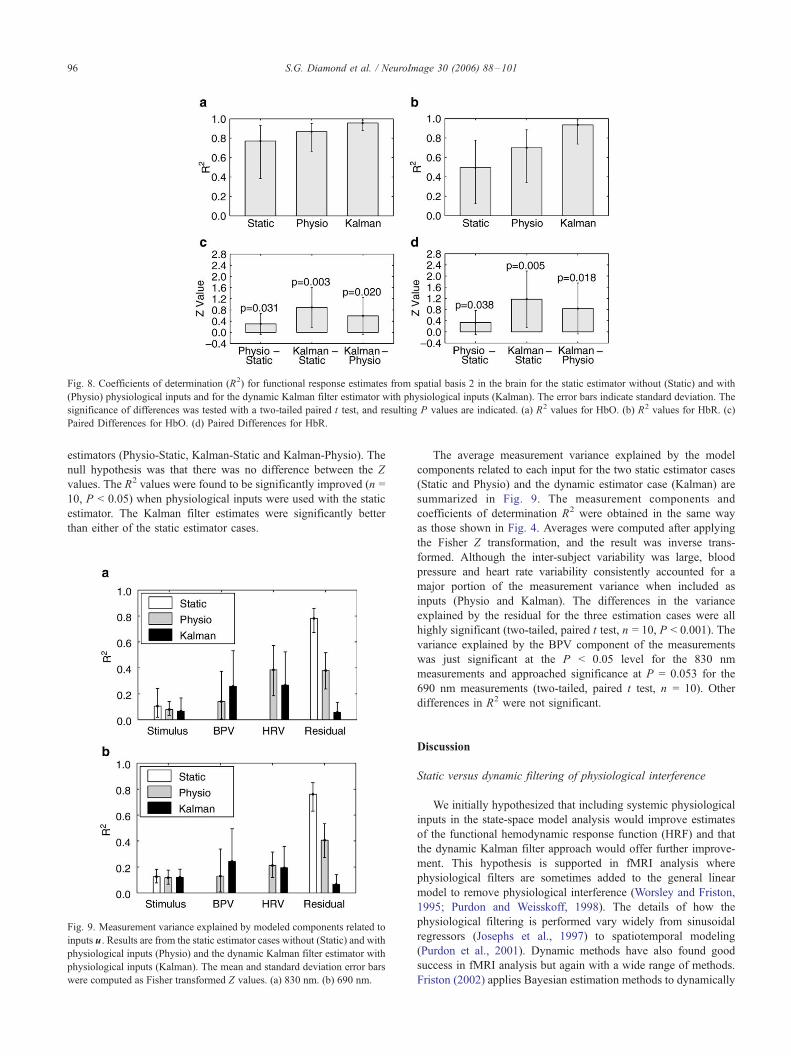
Fig. 8. Coefficients of determination (R2) for functional response estimates from spatial basis 2 in the brain for the static estimator without (Static) and with

(Physio) physiological inputs and for the dynamic Kalman filter estimator with physiological inputs (Kalman). The error bars indicate standard deviation. The

significance of differences was tested with a two-tailed paired t test, and resulting P values are indicated. (a) R2 values for HbO. (b) R2 values for HbR. (c)

Paired Differences for HbO. (d) Paired Differences for HbR.

S.G. Diamond et al. / NeuroImage 30 (2006) 88–10196

estimators (Physio-Static, Kalman-Static and Kalman-Physio). The

null hypothesis was that there was no difference between the Z

values. The R2 values were found to be significantly improved (n =

10, P < 0.05) when physiological inputs were used with the static

estimator. The Kalman filter estimates were significantly better

than either of the static estimator cases.

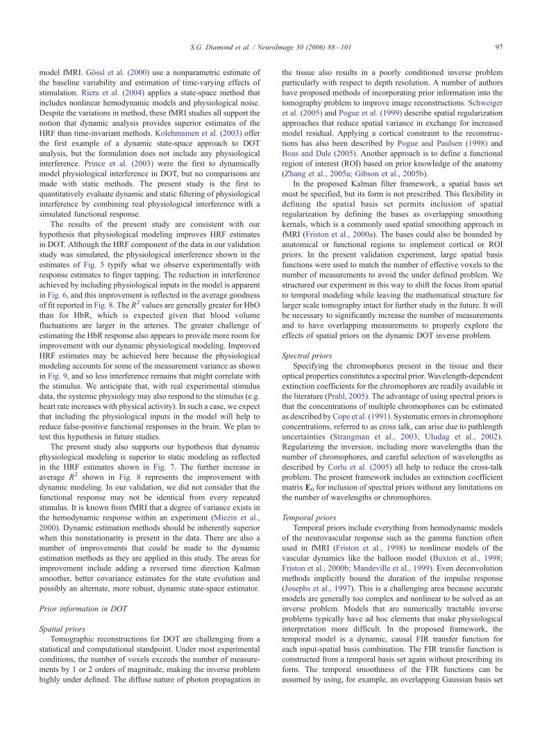
Fig. 9. Measurement variance explained by modeled components related to

inputs u. Results are from the static estimator cases without (Static) and with

physiological inputs (Physio) and the dynamic Kalman filter estimator with

physiological inputs (Kalman). The mean and standard deviation error bars

were computed as Fisher transformed Z values. (a) 830 nm. (b) 690 nm.

The average measurement variance explained by the model

components related to each input for the two static estimator cases

(Static and Physio) and the dynamic estimator case (Kalman) are

summarized in Fig. 9. The measurement components and

coefficients of determination R2 were obtained in the same way

as those shown in Fig. 4. Averages were computed after applying

the Fisher Z transformation, and the result was inverse trans-

formed. Although the inter-subject variability was large, blood

pressure and heart rate variability consistently accounted for a

major portion of the measurement variance when included as

inputs (Physio and Kalman). The differences in the variance

explained by the residual for the three estimation cases were all

highly significant (two-tailed, paired t test, n = 10, P < 0.001). The

variance explained by the BPV component of the measurements

was just significant at the P < 0.05 level for the 830 nm

measurements and approached significance at P = 0.053 for the

690 nm measurements (two-tailed, paired t test, n = 10). Other

differences in R2 were not significant.

Discussion

Static versus dynamic filtering of physiological interference

We initially hypothesized that including systemic physiological

inputs in the state-space model analysis would improve estimates

of the functional hemodynamic response function (HRF) and that

the dynamic Kalman filter approach would offer further improve-

ment. This hypothesis is supported in fMRI analysis where

physiological filters are sometimes added to the general linear

model to remove physiological interference (Worsley and Friston,

1995; Purdon and Weisskoff, 1998). The details of how the

physiological filtering is performed vary widely from sinusoidal

regressors (Josephs et al., 1997) to spatiotemporal modeling

(Purdon et al., 2001). Dynamic methods have also found good

success in fMRI analysis but again with a wide range of methods.

Friston (2002) applies Bayesian estimation methods to dynamically

S.G. Diamond et al. / NeuroImage 30 (2006) 88–101 97

model fMRI. Gossl et al. (2000) use a nonparametric estimate of

the baseline variability and estimation of time-varying effects of

stimulation. Riera et al. (2004) applies a state-space method that

includes nonlinear hemodynamic models and physiological noise.

Despite the variations in method, these fMRI studies all support the

notion that dynamic analysis provides superior estimates of the

HRF than time-invariant methods. Kolehmainen et al. (2003) offer

the first example of a dynamic state-space approach to DOT

analysis, but the formulation does not include any physiological

interference. Prince et al. (2003) were the first to dynamically

model physiological interference in DOT, but no comparisons are

made with static methods. The present study is the first to

quantitatively evaluate dynamic and static filtering of physiological

interference by combining real physiological interference with a

simulated functional response.

The results of the present study are consistent with our

hypothesis that physiological modeling improves HRF estimates

in DOT. Although the HRF component of the data in our validation

study was simulated, the physiological interference shown in the

estimates of Fig. 5 typify what we observe experimentally with

response estimates to finger tapping. The reduction in interference

achieved by including physiological inputs in the model is apparent

in Fig. 6, and this improvement is reflected in the average goodness

of fit reported in Fig. 8. The R2 values are generally greater for HbO

than for HbR, which is expected given that blood volume

fluctuations are larger in the arteries. The greater challenge of

estimating the HbR response also appears to provide more room for

improvement with our dynamic physiological modeling. Improved

HRF estimates may be achieved here because the physiological

modeling accounts for some of the measurement variance as shown

in Fig. 9, and so less interference remains that might correlate with

the stimulus. We anticipate that, with real experimental stimulus

data, the systemic physiology may also respond to the stimulus (e.g.

heart rate increases with physical activity). In such a case, we expect

that including the physiological inputs in the model will help to

reduce false-positive functional responses in the brain. We plan to

test this hypothesis in future studies.

The present study also supports our hypothesis that dynamic

physiological modeling is superior to static modeling as reflected

in the HRF estimates shown in Fig. 7. The further increase in

average R2 shown in Fig. 8 represents the improvement with

dynamic modeling. In our validation, we did not consider that the

functional response may not be identical from every repeated

stimulus. It is known from fMRI that a degree of variance exists in

the hemodynamic response within an experiment (Miezin et al.,

2000). Dynamic estimation methods should be inherently superior

when this nonstationarity is present in the data. There are also a

number of improvements that could be made to the dynamic

estimation methods as they are applied in this study. The areas for

improvement include adding a reversed time direction Kalman

smoother, better covariance estimates for the state evolution and

possibly an alternate, more robust, dynamic state-space estimator.

Prior information in DOT

Spatial priors

Tomographic reconstructions for DOT are challenging from a

statistical and computational standpoint. Under most experimental

conditions, the number of voxels exceeds the number of measure-

ments by 1 or 2 orders of magnitude, making the inverse problem

highly under defined. The diffuse nature of photon propagation in

the tissue also results in a poorly conditioned inverse problem

particularly with respect to depth resolution. A number of authors

have proposed methods of incorporating prior information into the

tomography problem to improve image reconstructions. Schweiger

et al. (2005) and Pogue et al. (1999) describe spatial regularization

approaches that reduce spatial variance in exchange for increased

model residual. Applying a cortical constraint to the reconstruc-

tions has also been described by Pogue and Paulsen (1998) and

Boas and Dale (2005). Another approach is to define a functional

region of interest (ROI) based on prior knowledge of the anatomy

(Zhang et al., 2005a; Gibson et al., 2005b).

In the proposed Kalman filter framework, a spatial basis set

must be specified, but its form is not prescribed. This flexibility in

defining the spatial basis set permits inclusion of spatial

regularization by defining the bases as overlapping smoothing

kernals, which is a commonly used spatial smoothing approach in

fMRI (Friston et al., 2000a). The bases could also be bounded by

anatomical or functional regions to implement cortical or ROI

priors. In the present validation experiment, large spatial basis

functions were used to match the number of effective voxels to the

number of measurements to avoid the under defined problem. We

structured our experiment in this way to shift the focus from spatial

to temporal modeling while leaving the mathematical structure for

larger scale tomography intact for further study in the future. It will

be necessary to significantly increase the number of measurements

and to have overlapping measurements to properly explore the

effects of spatial priors on the dynamic DOT inverse problem.

Spectral priors

Specifying the chromophores present in the tissue and their

optical properties constitutes a spectral prior.Wavelength-dependent

extinction coefficients for the chromophores are readily available in

the literature (Prahl, 2005). The advantage of using spectral priors is

that the concentrations of multiple chromophores can be estimated

as described byCope et al. (1991). Systematic errors in chromophore

concentrations, referred to as cross talk, can arise due to pathlength

uncertainties (Strangman et al., 2003; Uludag et al., 2002).

Regularizing the inversion, including more wavelengths than the

number of chromophores, and careful selection of wavelengths as

described by Corlu et al. (2005) all help to reduce the cross-talk

problem. The present framework includes an extinction coefficient

matrix E0 for inclusion of spectral priors without any limitations on

the number of wavelengths or chromophores.

Temporal priors

Temporal priors include everything from hemodynamic models

of the neurovascular response such as the gamma function often

used in fMRI (Friston et al., 1998) to nonlinear models of the

vascular dynamics like the balloon model (Buxton et al., 1998;

Friston et al., 2000b; Mandeville et al., 1999). Even deconvolution

methods implicitly bound the duration of the impulse response

(Josephs et al., 1997). This is a challenging area because accurate

models are generally too complex and nonlinear to be solved as an

inverse problem. Models that are numerically tractable inverse

problems typically have ad hoc elements that make physiological

interpretation more difficult. In the proposed framework, the

temporal model is a dynamic, causal FIR transfer function for

each input-spatial basis combination. The FIR transfer function is

constructed from a temporal basis set again without prescribing its

form. The temporal smoothness of the FIR functions can be

assumed by using, for example, an overlapping Gaussian basis set

S.G. Diamond et al. / NeuroImage 30 (2006) 88–10198

as in the present experiment. Even more constraints can be added

using an assumed time course for the hemodynamic response for

the basis set as described by Zhang et al. (2005c).

In a dynamic estimation framework, another category of

temporal priors is included that constrains the temporal evolution

of the states. In the present formulation, the states evolve as random

processes with a covariance prior. We used this covariance prior to

allow the BPV and HRV models to evolve more rapidly than the

functional response model. This had the effect of drawing more of

the random variance away from the functional response model and

improved the R2 values for the functional hemodynamics and

illustrates how priors are sometimes used as regularization

parameters. Some technical aspects of the dynamic priors in the

proposed Kalman filter framework could be more sophisticated. We

manually tuned the process noise covariance, but there are automatic

tuning procedures in the literature that may be appropriate for this

application (Kitagawa, 1998). Future implementations should also

include a state estimate smoother that operates in a reversed time

direction as described by Kaipio and Somersalo (2004). This will

help remove any lag in the state estimates and reduce the random

variance in the temporal evolution of the states.

Covariance between spatial, spectral and temporal priors

Additional benefit from prior information can be obtained by

modeling the co-variance between multiple priors. The benefits of

combined spatial and spectral priors have been demonstrated

previously (Li et al., 2005; Pogue and Paulsen, 1998). Zhang et al.

(2005c) combined spatial, spectral and temporal priors but only

with a time-invariant system model. In the proposed state-space

model, covariances between the spatial, spectral and temporal priors

are all included. We expect these covariances to improve the

tomographic reconstructions including possibly increased depth

resolution.

Anatomical and physiological models

Comprehensive DOT data analysis requires a biophysical

model of all the relevant anatomy and physiology formulated as

a numerically tractable inverse problem. Koyama et al. (2005) and

Boas et al. (2002) describe how DOT interacts with the anatomical

structure of the human head. Anatomical MRI is a useful prior for

DOT analysis (Barbour et al., 1995; Pogue and Paulsen, 1998;

Boas and Dale, 2005). DOT reveals the physiological dynamics in

hemoglobin concentration in the scalp and in the brain. Unraveling

these dynamics is a nontrivial inverse problem. A significant

advantage of a dynamic state-space approach for DOT analysis is

that it is particularly suitable to this class of inverse problems.

Arnold et al. (1998) provide an example of dynamic state-space

modeling of cardiac and respiratory interactions in the electro-

encephalogram (EEG).

If nonlinear models are used, then the extended Kalman filter is

an alternate formulation that facilitates dynamic parameter estima-

tion (Kailath et al., 2000). This research direction could extend to

integrating systems-level or large-scale neural modeling (Horwitz

et al., 1999) or dynamic causal modeling (Friston et al., 2003) with

the biophysics of DOT into a comprehensive inverse problem

formulation. Nonlinear circuit models are available to describe the

cardiovascular system (Mukkamala and Cohen, 2001), cerebral

autoregulation and gas exchange (Lu et al., 2003), vasomotion

(Ursino et al., 1998) and functional hemodynamics (Friston et al.,

2000b). A natural extension of this physiological modeling strategy

is to relate the biophysics of multiple imaging modalities that can be

performed simultaneously, such as DOT, EEG and fMRI, to a

common anatomical and physiological model. The physiologically

relevant parameters would then be estimated in a dynamic state-

space formulation.

Physiologically based interpretations of the neuroimaging data

offer advantages to neuroscience advancement and clinical applica-

tions. Identifying mechanical properties of the cerebral vasculature,

for example, could help to diagnose neurovascular pathologies like

those found in Alzheimer’s disease. Simultaneous fMRI and DOT

may help to illuminate the physiological dynamics of neurovascular

coupling that are the basis of hemodynamic neuroimaging (Buxton

et al., 1998; Friston et al., 2000b; Mandeville et al., 1999). We

designed the present state-space model as a first step toward

physiological interpretation of DOT and multimodal integration.

Extending to larger dimensional reconstruction

One of the practical challenges of dynamic state-space analysis in

DOT and other functional imaging technologies is the large

dimensionality of the data and analysis models. In the formulation

by Gossl et al. (2000), there are as many parameters to estimate as

there are observations for one effect. Large scale state-space

estimation is not a new challenge but is still an active area of

research. Khellah et al. (2005) provide an example of a new large-

scale technique from geophysics. The reduced rank square root

implementations of the Kalman filter are a notable method for

estimating otherwise unfeasibly large problems (Verlaan and

Heemink, 1997).

Although the proposed state-space approach was evaluated with

only a small spatial basis set, the same framework can be used for

problems of much larger spatial extent. The focus of the present

experiment was the temporal system identification aspect of DOT;

the spatial aspect will be examined in subsequent investigations.

Spatially overlapping and multi-distance measurements are also

desirable to fully utilize the tomography mathematics. Toward this

aim, the proposed state-space approach will accommodate time

domain multiplexing of the measurements (Boas et al., 2004a;

Bluestone et al., 2001), which is a requirement for collecting

measurements from source–detector separations that exceed the

limited dynamic range for the instrumentation. While dynamically

adjusting the detector gains permits an effective expansion of the

dynamic range, temporal gaps occur in the measurements. An

advantage of the proposed state-space model and Kalman filter

estimator is that these gaps in the data should be well tolerated.

Conclusion

Our state-space model for DOT analysis is purposefully

versatile, and so its implementation requires specification of

certain model elements. We frame a series of questions here as a

guide to using the proposed model. Who? Determine which

physiological and experimental inputs are important for the

analysis. Where? Specify the spatial basis set and photon

pathlength matrix for the anatomical structure. When? Specify

the temporal basis set for the finite impulse response models.

What? Estimate the states in the model. How? Determine how the

modeled components are related to functional anatomy and

physiology. Why? Hypothesize why the functional anatomy and

physiology is related to the model inputs.

S.G. Diamond et al. / NeuroImage 30 (2006) 88–101 99

The present work is only a step toward a comprehensive

dynamic framework for DOT data analysis and interpretation. The

proposed dynamic state-space approach has the potential to

significantly improve estimates of functional hemodynamics in

DOT neuroimaging and may open the door to a broader range of

brain activation paradigms. The ability to separate signals into

physiological components may reveal new information about the

local regulatory physiology and may be useful in identifying

certain vascular pathologies. Unlike the prior work with the

Kalman filter for DOT, the present formulation has the flexibility to

be applied to any experimental design and a broad range of spatial,

spectral and temporal priors. The proposed Kalman filter frame-

work may also be useful for other imaging modalities such as

fMRI, MEG and EEG or when multiple modalities are combined

with a single state-space model of the underlying physiology.

Acknowledgments

This work was supported by NIH T32-CA09502, P41-

RR14075, R01-EB001954 and the MIND Institute. The authors

would like to thank Professor Dana H. Brooks, Ph.D. of North-

eastern University for reviewing the manuscript and providing

insightful feedback.

References

Adelson, P.D., Nemoto, E., Scheuer, M., Painter, M., Morgan, J., Yonas, H.,

1999. Noninvasive continuous monitoring of cerebral oxygenation

periictally using near-infrared spectroscopy: a preliminary report.

Epilepsia 40, 1484–1489.

Arnold, M., Miltner, W.H.R., Witte, H., Bauer, R., Braun, C., 1998.

Adaptive AR modeling of nonstationary time series by means of

Kalman filtering. IEEE Trans. Biomed. Eng. 45 (5), 553–562.

Arridge, S.R., 1999. Optical tomography in medical imaging. Inverse Probl.

15, R41–R93.

Arridge, S.R., Cope, M., Delpy, D.T., 1992. The theoretical basis for the

determination of optical pathlengths in tissue: temporal and frequency

analysis. Phys. Med. Biol. 37, 1531–1560.

Baird, A.A., Kagan, J., Gaudette, T., Walz, K.A., Hershlag, N., Boas, D.A.,

2002. Frontal lobe activation during object permanence: data from near-

infrared spectroscopy. NeuroImage 16, 1120–1126.

Barbour, R.L., Graber, H.L., Chang, J., Barbour, S.S., Koo, P.C., Aronson,

R., 1995. MRI-guided optical tomography: prospects and computation

for a new imaging method. IEEE Comput. Sci. Eng. 2, 63–77.

Bluestone, A., Abdoulaev, G., Schmitz, C., Barbour, R., Hielscher, A.,

2001. Three-dimensional optical tomography of hemodynamics in the

human head. Opt. Express 9, 272–286.

Boas, D.A., Dale, A.M., 2005. Simulation study of magnetic resonance

imaging-guided cortically constrained diffuse optical tomography of

human brain function. Appl. Opt. 44 (10), 1957–1968.

Boas, D.A., Culver, J., Scott, J., Dunn, A.K., 2002. Three dimensional

Monte Carlo code for photon migration through complex heterogeneous

media including the adult head. Opt. Express 10, 159–170.

Boas, D.A., Chen, K., Grebert, D., Franceschini, M.A., 2004a. Improving

diffuse optical imaging spatial resolution of cerebral hemodynamic

response to brain activation in humans. Opt. Lett. 29, 1506–1508.

Boas, D.A., Dale, A.M., Franceschini, M.A., 2004b. Diffuse optical

imaging of brain activation: approaches to optimizing image sensitivity,

resolution and accuracy. NeuroImage 23, S275–S288.

Buxton, R.B., Wong, E.C., Frank, L.R., 1998. Dynamics of blood flow and

oxygenation changes during brain activation: the balloon model. Magn.

Reson. Med. 39 (6), 855–864.

Chandrasekhar, S., 1960. Radiative Transport. Dover, New York.

Chen, W.G., Li, P.C., Luo, Q.M., Zeng, S.Q., Hu, B., 2000. Hemodynamic

assessment of ischemic stroke with near-infrared spectroscopy. Space

Med. Med. Eng. (Beijing) 13, 84–89.

Chen, S., Sakatani, K., Lichty, W., Ning, P., Zhao, S., Zuo, H., 2002.

Auditory-evoked cerebral oxygenation changes in hypoxic– ischemic

encephalopathy of newborn infants monitored by near infrared spectro-

scopy. Early Hum. Dev. 67, 113–121.

Cohen, M.A., Taylor, J.A., 2002. Short-term cardiovascular oscillations in

man: measuring and modelling the physiologies. J. Physiol. 542 (Pt. 3),

669–683.

Colier, W.N., Quaresima, V., Oeseburg, B., Ferrari, M., 1999. Human

motor-cortex oxygenation changes induced by cyclic coupled move-

ments of hand and foot. Exp. Brain Res. 129, 457–461.

Cope, M., van der Zee, P., Essenpreis, M., Arridge, S.R., Delpy, D.T., 1991.

Data analysis methods for near infrared spectroscopy of tissue:

problems in determining the relative cytochrome aa3 concentration.

SPIE 1431, 251–262.

Corlu, A., Choe, R., Durduran, T., Lee, K., Schweiger, M., Arridge, S.R.,

Hillman, E.M.C., Yodh, A.G., 2005. Diffuse optical tomography with

spectral constraints and wavelength optimization. Appl. Opt. 44 (11),

2082–2093.

Dehghani, H., Pogue, B.W., Poplack, S.P., Paulsen, K.D., 2003. Multi-

wavelength three-dimensional near-infrared tomography of the breast:

initial simulation, phantom, and clinical results. Appl. Opt. 42 (1),

135–145.

Eschweiler, G.W., Wegerer, C., Schlotter, W., Spandl, C., Stevens, A.,

Bartels, M., Buchkremer, G., 2000. Left prefrontal activation predicts

therapeutic effects of repetitive transcranial magnetic stimulation

(rTMS) in major depression. Psychiatry Res. 99, 161–172.

Fallgatter, A.J., Strik, W.K., 2000. Reduced frontal functional asymmetry in

schizophrenia during a cued continuous performance test assessed with

near-infrared spectroscopy. Schizophr. Bull. 26, 913–919.

Fallgatter, A.J., Roesler, M., Sitzmann, L., Heidrich, A., Mueller, T.J., Strik,

W.K., 1997. Loss of functional hemispheric asymmetry in Alzheimer’s

dementia assessed with near-infrared spectroscopy. Brain Res. Cogn.

Brain Res. 6, 67–72.

Frackowiak, R.S.J., Friston, K.J., Frith, C., Dolan, R., Price, C.J., Zeki,

S., Ashburner, J., Penny, W.D. (Eds.), 2003. Human Brain Function,

2nd ed. Academic Press. URL http://www.fil.ion.ucl.ac.uk/spm/doc/

books/hbf2/.

Franceschini, M.A., Fantini, S., Thompson, J.H., Culver, J.P., Boas, D.A.,

2003. Hemodynamic evoked response of the sensorimotor cortex

measured non-invasively with near-infrared optical imaging. Psycho-

physiology 40, 548–560.

Friston, K.J., 2002. Bayesian estimation of dynamical systems: an

application to fMRI. NeuroImage 16, 513–530.

Friston, K.J., Fletcher, P., Josephs, O., Holmes, A., Rugg, M.D., Turner, R.,

1998. Event-related fMRI: characterizing differential responses. Neuro-

Image 7, 30–40.

Friston, K.J., Josephs, O., Zarahn, E., Holmes, A.P., Rouquette, S., Poline,

J.B., 2000a. To smooth or not to smooth? Bias and efficiency in fMRI

time-series analysis. NeuroImage 12 (2), 196–208.

Friston, K.J., Mechelli, A., Turner, R., Price, C.J., 2000b. Nonlinear

responses in fMRI: the Balloon model, Volterra kernels, and other

hemodynamics. NeuroImage 12 (4), 466–477.

Friston, K.J., Harrison, L., Penny, W., 2003. Dynamic causal modelling.

NeuroImage 19 (4), 1273–1302.

Fukui, Y., Ajichi, Y., Okada, E., 2003. Monte Carlo prediction of near-

infrared light propagation in realistic adult and neonatal head models.

Appl. Opt. 42 (16), 2881–2887.

Gibson, A.P., Hebden, J.C., Arridge, SR., 2005a. Recent advances in

diffuse optical imaging. Phys. Med. Biol. 50, R1–R43.

Gibson, A.P., Hebden, J.C., Riley, J., Everdell, N., Schweiger, M., Arridge,

S.R., Delpy, D.T., 2005b. Linear and nonlinear reconstruction for

optical tomography of phantoms with nonscattering regions. Appl. Opt.

44 (19), 3925–3936.

S.G. Diamond et al. / NeuroImage 30 (2006) 88–101100

Gossl, C., Auer, D.P., Fahrmeir, L., 2000. Dynamic models in fMRI. Magn.

Reson. Med. 43, 72–81.

Goutte, C., Nielsen, F.A., Hansen, L.K., 2000. Modeling the haemody-

namic response in fMRI using smooth FIR filters. IEEE Trans. Med.

Imag. 19 (12), 1188–1201.

Hanlon, E.B., Itzkan, I., Dasari, R.R., Feld, M.S., Ferrante, R.J., McKee,

A.C., Lathi, D., Kowall, N.W., 1999. Near-infrared fluorescence

spectroscopy detects Alzheimer’s disease in vitro. Photochem. Photo-

biol. 70, 236–242.

Hayashi, T., Kashio, Y., Okada, E., 2003. Hybrid Monte Carlo-diffusion

method for light propagation in tissue with a low-scattering region.

Appl. Opt. 42 (16), 2888–2896.

Hebden, J.C., Gibson, A., Austin, T., Yusof, R.M., Everdell, N.,

Delpy, D.T., Arridge, S.R., Meek, J.H., Wyatt, J.S., 2004. Imaging

changes in blood volume and oxygenation in the newborn infant

brain using three-dimensional optical tomography. Phys. Med. Biol.

49 (7), 1117–1130.

Hintz, S.R., Benaron, D.A., Siegel, A.M., Zourabian, A., Stevenson, D.K.,

Boas, D.A., 2001. Bedside functional imaging of the premature infant

brain during passive motor activation. J. Perinat. Med. 29 (4), 335–343.

Hock, C., Villringer, K., Muller-Spahn, F., Hofmann, M., Schuh-Hofer, S.,

Heekeren, H., Wenzel, R., Dirnagl, U., Villringer, A., 1996. Near

infrared spectroscopy in the diagnosis of Alzheimer’s disease. Ann.

N. Y. Acad. Sci. 777, 22–29.

Horwitz, B., Tagamets, M.A., McIntosh, A.R., 1999. Neural modeling,

functional brain imaging, and cognition. Trends Cogn. Sci. 3 (3),

91–98.

Jakubowski, D.B., Cerussi, A.E., Bevilacqua, F., Shah, N., Hsiang, D.,

Butler, J., Tromberg, B.J., 2004. Monitoring neoadjuvant chemotherapy

in breast cancer using quantitative diffuse optical spectroscopy: a case

study. J. Biomed. Opt. 9 (1), 230–238.

Josephs, O., Turner, R., Friston, K., 1997. Event-related fMRI. Hum. Brain

Mapp. 5 (4), 243–248.

Kailath, T., Sayed, A.H., Hassibi, B., 2000. Linear estimation. Information

and System Sciences. Prentice-Hall.

Kaipio, J.P., Somersalo, E., 2004. Statistical and Computational Inverse

Problems, Applied Mathematical Sciences, vol. 160. Springer-Verlag.

Kalman, R.E., 1960. A new approach to linear filtering and prediction

problems. Trans. ASME—J. Basic Eng. 82, 35–45.

Kay, S.M., 1993. Fundamentals of Statistical Signal Processing, Estimation

Theory. Prentice Hall.

Khellah, F., Fieguth, P., Murray, M.J., Allen, M., 2005. Statistical

processing of large image sequences. IEEE Trans. Image Process. 14

(1), 80–93.

Kitagawa, G., 1998. A self-organizing state-space model. J. Am. Stat.

Assoc. 93 (443), 1203–1215.

Kolehmainen, V., Prince, S., Arridge, S., Kaipio, J., 2003. State-estimation

approach to the nonstationary optical tomography problem. J. Opt. Soc.

Am. A 20 (5), 876–889.

Koyama, T., Iwasaki, A., Ogoshi, Y., Okada, E., 2005. Practical and

adequate approach to modeling light propagation in an adult head with

low-scattering regions by use of diffusion theory. Appl. Opt. 44 (11),

2094–2103.

Li, A., Boverman, G., Zhang, Y., Brooks, D., Miller, E.L., Kilmer, M.E.,

Zhang, Q., Hillman, E.M.C., Boas, D.A., 2005. Optimal linear inverse

solution with multiple priors in diffuse optical tomography. Appl. Opt.

44 (10), 1948–1956.

Logothetis, N.K., Pauls, J., Augath, M., Trinath, T., Oeltermann, A., 2001.

Neurophysiological investigation of the basis of the fMRI signal. Nature

412 (6843), 150–157.

Lu, K., Clark Jr., J.W., Ghorbel, F.H., Ware, D.L., Zwischenberger, J.B.,

Bidani, A., 2003. Whole-body gas exchange in human predicted by a

cardiopulmonary model. Cardiovasc. Eng. Int. J. 3 (1), 1–19.

Lu, K., Clark Jr., J.W., Ghorbel, F.H., Robertson, C.S., Ware, D.L.,

Zwischenberger, J.B., Bidani, A., 2004. Cerebral autoregulation and gas

exchange studied using a human cardiopulmonary model. Am. J.

Physiol.: Heart Circ. Physiol. 286, H584–H601.

Mandeville, J.B., Marota, J.J., Ayata, C., Zaharchuk, G., Moskowitz, M.A.,

Rosen, B.R., Weisskoff, R.M., 1999. Evidence of a cerebrovascular

postarteriole windkessel with delayed compliance. J. Cereb. Blood Flow

Metab. 19 (6), 679–689.

Matsuo, K., Kato, T., Fukuda, M., Kato, N., 2000. Alteration of hemoglobin

oxygenation in the frontal region in elderly depressed patients as

measured by near-infrared spectroscopy. J. Neuropsychiatry Clin.

Neurosci. 12, 465–471.

Mayhew, J.E.W., Askew, S., Zheng, Y., Porrill, J., Westby, G.W.M.,

Redgrave, P., Rector, D.M., Harper, R.M., 1996. Cerebral vasomotion:

a 0.1-Hz oscillation in reflected light imaging of neural activity.

NeuroImage 4, 183–193.

Meek, J.H., Elwell, C.E., McCormick, D.C., Edwards, A.D., Townsend,

J.P., Steward, A.L., Wyatt, J.S., 1999. Abnormal cerebral haemody-

namics in perinatally asphyxiated neonates related to outcome. Arch.

Dis. Child. 81, F110–F115.

Miezin, F.M., Maccotta, L., Ollinger, J.M, Petersen, S.E., Buckner, R.L.,

2000. Characterizing the hemodynamic response: effects of presentation

rate, sampling procedure, and the possibility of ordering brain activity

based on relative timing. NeuroImage 11 (6), 735–759 (Part 1).

Mukkamala, R., Cohen, R.J., 2001. A forward model-based validation of

cardiovascular system identification. Am. J. Physiol.: Heart Circ.

Physiol. 281, H2714–H2730.

Nemoto, E.M., Yonas, H., Kassam, A., 2000. Clinical experience with

cerebral oximetry in stroke and cardiac arrest. Crit. Care Med. 28,

1052–1054.

Obrig, H., Neufang, M., Wenzel, R., Kohl, M., Steinbrink, J., Einhaupl, K.,

Villringer, A., 2000. Spontaneous low frequency oscillations of cerebral

hemodynamics and metabolism in human adults. NeuroImage 12 (6),

623–639.

Okada, F., Tokumitsu, Y., Hoshi, Y., Tamura, M., 1994. Impaired

interhemispheric integration in brain oxygenation and hemodynam-

ics in schizophrenia. Eur. Arch. Psychiatry Clin. Neurosci. 244,

17–25.

Okada, E., Schweiger, M., Arridge, S.R., Firbank, M., Delpy, D.T., 1996a.

Experimental validation of Monte Carlo and finite-element methods of

estimation of the optical path length in inhomogeneous tissue. Appl.

Opt. 35 (19), 3362–3371.

Okada, F., Takahashi, N., Tokumitsu, Y., 1996b. Dominance of the

Fnondominant_ hemisphere in depression. J. Affective Disord. 37,

13–21.

Panerai, R.B., 2004. System identification of human cerebral blood flow

regulatory mechanisms. Cardiovasc. Eng. Int. J. 4 (1), 59–71.

Pena, M., Maki, A., Kovacic, D., Dehaene-Lambertz, G., Koizumi, H.,

Bouquet, F., Mehler, J., 2003. Sounds and silence: an optical top-

ography study of language recognition at birth. Proc. Natl. Acad. Sci.

100, 11702–11705.

Pogue, B.W., Paulsen, K.D., 1998. High-resolution near-infrared tomo-

graphic imaging simulations of the rat cranium by use of a priori

magnetic resonance imaging structural information. Opt. Lett. 23,

1716–1718.

Pogue, B.W., McBride, T.O., Prewitt, J., Osterberg, U.L., Paulsen, K.D.,

1999. Spatially variant regularization improves diffuse optical tomog-

raphy. Appl. Opt. 38, 2950–2961.

Prahl, S., 2005. Tabulated molar extinction coefficient for hemoglobin in

water. Oregon Medical Laser Center. URL http://omlc.ogi.edu/spectra/

hemoglobin/summary.html.

Prince, S., Kolehmainen, V., Kaipio, J.P., Franceschini, M.A., Boas, D.A.,

Arridge, S.R., 2003. Time-series estimation of biological factors in

optical diffusion tomography. Phys. Med. Biol. 48, 1491–1504.

Purdon, P.L., Weisskoff, R.M., 1998. Effect of temporal autocorrelation due

to physiological noise and stimulus paradigm on voxel-level false-

positive rates in fMRI. Hum. Brain Mapp. 6 (4), 239–249.

Purdon, P.L., Solo, V., Weisskoff, R.M., Brown, E.N., 2001. Locally

regularized spatiotemporal modeling and model comparison for func-

tional MRI. NeuroImage 14 (4), 912–923.

Riera, J.J., Watanabe, J., Kazuki, I., Naoki, M., Aubert, E., Ozaki, T.,

S.G. Diamond et al. / NeuroImage 30 (2006) 88–101 101

Kawashima, R., 2004. A state-space model of the hemodynamic ap-

proach: nonlinear filtering of BOLD signals. NeuroImage 21, 547–567.

Ripoll, J., Arridge, S.R., Nieto-Vesperinas, M., 2001. Effect of roughness in

non-diffusive regions within diffusive media. J. Opt. Soc. Am. A 18,

940–947.

Rostrup, E., Law, I., Pott, F., Ide, K., Knudsen, G.M., 2002. Cerebral

hemodynamics measured with simultaneous PET and near-infrared

spectroscopy in humans. Brain Res. 954 (2), 183–193.

Ruben, J., Wenzel, R., Obrig, H., Villringer, K., Bernarding, J., Hirth, C.,

Heekeren, H., Dirnagl, U., Villringer, A., 1997. Haemoglobin oxygen-

ation changes during visual stimulation in the occipital cortex. Adv.

Exp. Med. Biol. 428, 181–187.

Saitou, H., Yanagi, H., Hara, S., Tsuchiya, S., Tomura, S., 2000. Cerebral

blood volume and oxygenation among poststroke hemiplegic patients:

effects of 13 rehabilitation tasks measured by near-infrared spectro-

scopy. Arch. Phys. Med. Rehabil. 81, 1348–1356.

Sakatani, K., Chen, S., Lichty, W., Zuo, H., Wang, Y.P., 1999. Cerebral

blood oxygenation changes induced by auditory stimulation in newborn

infants measured by near infrared spectroscopy. Early Hum. Dev. 55,

229–236.

Sato, H., Takeuchi, T., Sakai, K.L., 1999. Temporal cortex activation

during speech recognition: an optical topography study. Cognition 73,

B55–B66.

Schweiger, M., Arridge, S.R., Nissila, I., 2005. Gauss–Newton method for

image reconstruction in diffuse optical tomography. Phys. Med. Biol. 50

(10), 2365–2386.

Shah, N., Cerussi, A.E., Jakubowski, D., Hsiang, D., Butler, J., Tromberg,

B.J., 2004. Spatial variations in optical and physiological properties of

healthy breast tissue. J. Biomed. Opt. 9 (3), 534–540.

Sokol, D.K., Markand, O.N., Daly, E.C., Luerssen, T.G., Malkoff, M.D.,

2000. Near infrared spectroscopy (NIRS) distinguishes seizure types.

Seizure 9, 323–327.

Srinivasan, S., Pogue, B.W., Jiang, S., Dehghani, H., Kogel, C., Soho, S.,

Gibson, J.J., Tosteson, T.D., Poplack, S.P., Paulsen, K.D., 2003.

Interpreting hemoglobin and water concentration, oxygen saturation,

and scattering measured in vivo by near-infrared breast tomography.

Proc. Natl. Acad. Sci. 100 (21), 12349–12354.

Steinhoff, B.J., Herrendorf, G., Kurth, C., 1996. Ictal near infrared

spectroscopy in temporal lobe epilepsy: a pilot study. Seizure 5, 97–101.

Strangman, G., Culver, J.P., Thompson, J., Boas, D.A., 2002. A quantitative

comparison of simultaneous BOLD fMRI and NIRS recordings during

functional brain activation. NeuroImage 17, 719–731.

Strangman, G., Franceschini, M.A., Boas, D.A., 2003. Factors affecting the

accuracy of near-infrared spectroscopy concentration calculations for

focal changes in oxygenation parameters. NeuroImage 18, 865–879.

Taga, G., Asakawa, K., Maki, A., Konishi, Y., Koizumi, H., 2003. Brain

imaging in awake infants by near-infrared optical topography. Proc.

Natl. Acad. Sci. 100, 10722–10727.

Toronov, V., Franceschini, M., Filiaci, M., Fantini, S., Wolf, M., Michalos,

A., Gratton, E., 2000. Near-infrared study of fluctuations in cerebral

hemodynamics during rest and motor stimulation: temporal analysis and

spatial mapping. Med. Phys. 27 (4), 801–815.

Uludag, K., Kohl, M., Steinbrink, J., Obrig, H., Villringer, A., 2002. Cross

talk in the Lambert–Beer calculation for near-infrared wavelengths

estimated by Monte Carlo simulations. J. Biomed. Opt. 7, 51–59.

Ursino, M., Colantuoni, A., Bertuglia, S., 1998. Vasomotion and blood flow

regulation in hamster skeletal muscle microcirculation: a theoretical and

experimental study. Microvasc. Res. 56, 233–252.

Verlaan, M., Heemink, A.W., 1997. Tidal flow forecasting using reduced

rank square root filters. Stoch. Hydrol. Hydraul. 5, 349–368.

Vernieri, F., Rosato, N., Pauri, F., Tibuzzi, F., Passarelli, F., Rossini, P.M.,

1999. Near infrared spectroscopy and transcranial Doppler in mono-

hemispheric stroke. Eur. Neurol. 41, 159–162.

Watanabe, E., Maki, A., Kawaguchi, F., Yamashita, Y., Koizumi, H.,

Mayanagi, Y., 2000. Noninvasive cerebral blood volume measurement

during seizures using multichannel near infrared spectroscopic top-

ography. J. Biomed. Opt. 5, 287–290.

Worsley, K.J., Friston, K.J., 1995. Analysis of fMRI time-series revisited-

again. NeuroImage 2 (3), 173–181.

Xu, H., Springett, R., Dehghani, H., Pogue, B.W., Paulsen, K.D., Dunn,

J.F., 2005. Magnetic-resonance-imaging-coupled broadband near-infra-

red tomography system for small animal brain studies. Appl. Opt. 44

(11), 2177–2188.

Yamamoto, T., Maki, A., Kadoya, T., Tanikawa, Y., Yamada, Y., Okada,

E., Koizumi, H., 2002. Arranging optical fibres for the spatial re-

solution improvement of topographical images. Phys. Med. Biol. 47,

3429–3440.

Zhang, Q., Brukilacchio, T.J., Li, A., Stott, J., Chaves, T., Hillman, E., Wu,

T., Chorlton, M., Rafferty, E., Moore, R.H., Kopans, D.B., Boas, D.A.,

2005a. Coregistered tomographic X-ray and optical breast imaging:

initial results. J. Biomed. Opt. 10 (2), 024033.

Zhang, Y., Brooks, D.H., Franceschini, M.A., Boas, D.A., 2005b.

Eigenvector-based spatial filtering for reduction of physiological

interference in diffuse optical imaging. J. of Biomed. Opt. 10 (1),

011014.

Zhang, Y., Brooks, D.H., Boas, D.A., 2005c. A hemodynamic response

function model in spatio-temporal diffuse optical tomography. Phys.

Med. Biol. 50 (19), 4625–4644.

Zwiener, U., Schelenz, C., Bramer, S., Hoyer, D., 2001. Short-term

dynamics of relative coordination between respiratory movements,

heart rate and arterial pressure fluctuations within the respiratory

frequency range. Physiol. Res. 50, 59–69.