Embed Size (px)
Citation preview
JSS Journal of Statistical SoftwareMay 2013, Volume 53, Issue 11. http://www.jstatsoft.org/
A Distributed Procedure for Computing Stochastic
Expansions with Mathematica
Christophe LadroueUniversity of Warwick
Anastasia PapavasiliouUniversity of Warwick
Abstract
The solution of a (stochastic) differential equation can be locally approximated by a(stochastic) expansion. If the vector field of the differential equation is a polynomial, thecorresponding expansion is a linear combination of iterated integrals of the drivers andcan be calculated using Picard Iterations. However, such expansions grow exponentiallyfast in their number of terms, due to their specific algebra, rendering their practical uselimited.
We present a Mathematica procedure that addresses this issue by reparametrizing thepolynomials and distributing the load in as small as possible parts that can be processedand manipulated independently, thus alleviating large memory requirements and beingperfectly suited for parallelized computation. We also present an iterative implementationof the shuffle product (as opposed to a recursive one, more usually implemented) as well asa fast way for calculating the expectation of iterated Stratonovich integrals for Brownianmotion.
Keywords: rough paths, stochastic expansion, iterated integral, picard iteration, simulation,Mathematica.
1. Motivation and mathematical background
In this section, we introduce the mathematical background and motivation for manipulat-ing expansions and iterated integrals. The next subsection introduces the Picard procedure,a simple iterative way to derive local approximation of the solution of a differential equa-tion. Iterated integrals are then introduced and the two are finally combined to define theexpansions.
2 A Distributed Procedure for Stochastic Expansions in Mathematica
1.1. Motivation and notation
Consider the following stochastic differential equation (SDE):
dYt = f(Yt, θ)dXt (1)
where Yt ∈ Rm, Xt ∈ Rn and f(., θ) ∈ Rm×n. The parameters of the function f are collectedin the variable θ. We call each X(i) a driver of the differential equation. We assume thefunctions fj,i, i ∈ {1 . . . n}, j ∈ {1 . . .m} to be polynomials. The initial value of Yt is set toY0.
The objective is to derive a local approximation of the solution in terms of f , Y0 and theiterated integrals of Yt, i.e., that is integrals of the form∫
. . .
∫0<u1<···<uk≤T
dXτ1u1 . . . dX
τkuk
for any word τ = (τ1, . . . , τk) constituted of the letter τi ∈ {1, . . . , n}, i = 1, . . . , k.. Suchexpansions play an important role in the theory of rough paths, allowing one to define sucha differential equation for a large class of drivers X (Lyons and Qian 2003). They have alsobeen used recently for parameter estimation of SDE (Papavasiliou and Ladroue 2010).
Iterated integrals have been implemented in Mathematica before. Kendall (2005) showed howto manipulate stochastic integrals symbolically by implementing the rules of Ito calculus.Their package Itosvn3 could also compute analytic forms of the expectation of stochasticintegrals. For example, once the user provided the solution of an SDE in terms of stochasticintegrals, its moments could be calculated. In this paper’s setting however, the solution isnot known and is analytically approximated with Stratonovitch calculus. Tocino (2009) pre-sented an implementation of iterated integral calculus that realized both Ito and Stratonovitchvariants and used it to derive a number of new relations for iterated integrals products andpowers. However, as the number of terms to consider grows exponentially with every product,this implementation will not scale up.
1.2. Picard iterations
Picard iterations provide a way for deriving local approximations of solutions of differentialequation. They are defined as:
Y0,T (0) = Y0 − Y0 = 0 (2)
Y0,T (r + 1, j) =n∑i=1
∫fj,i(Ys(r, j))dX
(i)s (3)
(4)
where Y0,T (r, j) is the j-th component of the approximation of Y0,T =∫ T0 dYs = YT −Y0 after
r iterations. Thus, the first iteration gives:
Y0,T (1, j) =
∫ t
0fj,1(Y0)dX
(1)s + . . .+
∫ t
0fj,n(Y0)dX
(n)s (5)
Note that if we are interested in the actual value of the solution at a time t ∈ [0, T ], its Picardapproximation is given by
Yt(r, j) = Y0 + Y0,t(r, j).
Journal of Statistical Software 3
One of the main successes in the theory of rough paths was to give precise conditions on Xand f for Picard iterations to converge (Lyons and Qian 2003).
1.3. Iterated integrals
Iterated integrals are integrals of the form:
X(τ)s,t =
∫. . .
∫s<u1<...<uk<t
dX(τ1)u1 . . . dX(τk)
uk
where τ = (τ1, . . . , τk) is called a word, with letters τi ∈ {1 . . . n}, i = 1, . . . , k. By definition,integrating an iterated integral produces an iterated integral:∫ T
0X
(τ)0,s dX
(j)s =
∫ T
0
∫. . .
∫0<u1<...<uk<s
dX(τ1)u1 . . . dX(τk)
ukdX(j)
s (6)
= X(τ1,...,τk,j)0,T (7)
If X is a geometric p-rough path, i.e., it can be approximated by paths of bounded varia-tion (see Lyons and Qian (2003) for a precise definition), then the integrals obey the usualintegration-by-parts rule, which can be generalized as follows:
X(τ)s,t X
(ρ)s,t =
∑α∈τtρ
X(α)s,t (8)
The shuffle product t of two words τ and ρ is the set of all words using the letters in τ and ρsuch that they are in their original order. For example 13t42 = {1342, 1432, 4132, 1423, 4213,4132} but 1324, for example, does not belong to the set.
This result holds only in the case of deterministic drivers X, or Stratonovitch integrals. Asimilar relation exists for Ito integrals but requires a small correcting term (Tocino 2009)making them slightly less practical in this context. A simple transformation allows diffusionprocesses to be defined with respect to Ito or Stratonovitch integrals (Kloeden and Platen1991):
dyt = µ(yt)dt+ σ(yt)dBt ⇔ dyt =
(µ(yt)−
1
2σ′(yt)σ(yt)
)dt+ σ(yt) ◦ dBt
It immediately follows from Equation 8 that any power of an iterated integral is a sum ofiterated integrals and that a polynomial of iterated integrals is also a linear combination ofsingle iterated integrals. For example:
X(1)0,TX
(2,3)0,T = X
(1,2,3)0,T +X
(2,1,3)0,T +X
(2,3,1)0,T(
X(1)0,T
)2= X
(1)0,TX
(1)0,T
= X(1,1)0,T +X
(1,1)0,T
= 2X(1,1)0,T(
X(1)0,T
)`= `! X
(1,...,1)0,T
X(0,1,0)0,T X
(1,1)0,T = X
(0,1,0,1,1)0,T + 2X
(0,1,1,0,1)0,T + 3X
(0,1,1,1,0)0,T
+X(1,0,1,0,1)0,T + 2X
(1,0,1,1,0)0,T +X
(1,1,0,1,0)0,T
4 A Distributed Procedure for Stochastic Expansions in Mathematica
The number of terms from the product of iterated integrals grows fast, exponentially if allletters are different.
1.4. Expansions
We are now in position to derive expansions for the solution of a differential equation. Picarditerations yield:
Y0,T (0, j) = 0
Y0,T (1, j) =
∫0,T
fj1(Ys(0))dX(1)s + . . .+
∫0,T
fjn(Ys(0))dX(n)s
= fj1(Y0)X(1)0,T + . . .+ fjn(Y0)X
(n)0,T
Y0,T (2, j) =
∫0,T
fj1(Ys(1))dX(1)s + . . .+
∫0,T
fjn(Ys(1))dX(n)s
=
∫0,T
fj1(Y0,s(1) + Y0)dX(1)s + . . .+
∫0,T
fjn(Ys(1) + Y0)dX(n)s
Since Y0,s(1, .) is a sum of iterated integrals, the polynomials fji(Ys(1) + Y0) are also sumsof iterated integrals and so is their integration with respect to X(i). Y0,T (2) is thus a sum ofiterated integrals and by recursion all Y0,T (r, .) are. A formal proof in the context of differentialequations driven by rough paths can be found in Papavasiliou and Ladroue (2010).
Example
Consider the Ornstein-Uhlenbeck process: dyt = a(1− yt)dt+ bdWt and y0 = 0. In this case,
X(1)t = t, X
(2)t = Wt and Y
(i)0 = 0 for i ∈ {1, 2}. Applying Picard iterations, we obtain:
Y0,T (0) = 0
Y0,T (1) =
∫ T
0a(1− 0)dX(1)
s +
∫ T
0bdX(2)
s
= aX(1)0,T + bX
(2)0,T
Y0,T (2) =
∫ T
0a(1− (aX(1)
s + bX(2)s ))dX(1)
s +
∫ T
0bdX(2)
s
= aX(1)0,T − a
2X(1,1)0,T − abX
(2,1)0,T + bX
(2)0,T
Y0,T (3) = aX(1)0,T − a
2X(1,1)0,T + a3X
(1,1,1)0,T + abX
(2,1,1)0,T + abX
(2,1)0,T + bX
(2)0,T
The solution of the stochastic differential equation can thus be approximated by a seriesof iterated integral of the drivers, whose coefficients are a function of the parameters. Theiterated integrals capture the statistics of the drivers and are separated from the parameters.
This derivation can be readily implemented in Mathematica (Wolfram 2003) – see Tocino(2009) for an implementation of the shuffle product – but suffers a major drawback: eachproduct of iterated integrals being a shuffle product, the number of terms produced growsextremely fast (exponentially in the worst cases) and rapidly becomes unmanageable. In thenext section, we introduce a reparametrization of the problem that circumvents this problemby providing an alternative representation of the expansion which can be processed in adistributed manner, alleviating large memory requirements.
Journal of Statistical Software 5
2. Reparametrization of the polynomials
One thing to note in the derivation of expansions is that each successive iterations requires theexplicit linear combination of iterated integrals for the previous iteration; evaluating Y0,T (r)requires the complete expansion for Y0,T (r−1). As the number of terms grows, manipulatingthis object rapidly becomes unwieldy.
In this section, we describe a reparametrization of the polynomials which bypasses the needfor an expansion in terms of iterated integrals. It provides a more compact representationof the approximate solution and is naturally amenable to parallel processing. For clarityof exposition, we first introduce the approach in the case of a one-dimensional (m = 1)differential equation with n drivers. We assume the polynomials f1i to be of degree less orequal to q. In the last subsection, the procedure is generalized to m-dimensional differentialequations.
2.1. One-dimensional case
We first remark that a polynomial P (y) can be written in terms of y−y0 by writing its Taylorexpansion around y0:
P (y) =
q∑k=0
1
k!∂kP (y0)(y − y0)k (9)
Next we introduce the following new operation for iterated integrals:
Xαs,t B Xβ
s,t =
∫ t
sXαs,udX
βs,u =
∫ t
sXαs,uX
β−s,udX
βendu (10)
where β− is the word β with the last letter removed and βend the last letter of β. This is anon-associative, non-commutative operation – in fact, it can be viewed as a non-commutativedendriform. We can rewrite the Picard iteration using this operation. Note that from nowon, the interval [s, t] will be fixed to [0, T ] and will be omitted.
Y (0) = y0 − y0 = 0 (11)
Y (1) =n∑i=1
∫ T
0fj1(Ys(0) + y0)dX
(i)s (12)
=n∑i=1
fj1(y0)X(i) (13)
Y (r + 1) =
n∑i=1
f1i(Ys(r) + y0) B X(i) (14)
=n∑i=1
q∑k=0
1
k!∂kf1i(y0)Ys(r)
k B X(i) (15)
=
q∑k=0
(((Ys(r))
k Bn∑i=1
(∂kf1i(y0)X(i))
)(16)
Therefore, if we define the objects Q as:
Qk =n∑i=1
1
k!∂kf1i(y0)X
(i), (17)
6 A Distributed Procedure for Stochastic Expansions in Mathematica
the Picard iteration takes the following form:
Y (1) = Q0
Y (r + 1) =
q∑k=0
Y (r)k B Qk
where Y (r)k is the usual product.
2.2. Description of the approach
Consider a one-dimensional differential equation with quadratic functions f1i, i.e., q = 2. Thenew representation yields:
Y (1) = Q0 (18)
Y (2) = 1 B Q0 +Q0 B Q1 + (Q0)2 B Q2 (19)
= Q0 +Q0 B Q1 + (Q0)2 B Q2 (20)
Y (3) = Q0 + (Q0 +Q0 B Q1 + (Q0)2 B Q2) B Q1 (21)
+(Q0 +Q0 B Q1 + (Q0)2 B Q2)2 B Q2 (22)
where (Qk)` is the k-th object Q to the power `. Crucially, this new representation does notrequire the explicit computation of the shuffle products, keeping the number of terms undercontrol. Moreover, the expression can be expanded into its summands and each summand beprocessed independently. Thus, we avoid the handling of a large expression and are able toparallelize the computation.
Note that the representation only depends on the maximum degree of the polynomials butnot on the number of drivers. The Picard iteration can therefore be done only once, storedin a file and used at a later date for any system that uses the same maximum degree q.
Using this representation, it is possible to derive the stochastic expansions through a fewstages:
1. Expand the expression Y (r) into its monomials u. Each monomial u is a function of Q’sthat uses the non-commutative products. Importantly, the objects Q and the productB are only used as place-holders at that stage. For example, the first three monomialsfor Y (3) are Q0, Q0 B Q1 and (Q0 B Q1) B Q1.
2. For each monomial u, the objects Q are replaced by their values from the model athand. Each Q is a weighted sum of the drivers X(i) (Equation 17), so each u becomesa polynomial V of X(i) in terms of the non-commutative product. As in the previousstep, the product is still only employed as a place-holder and not instantiated.
3. Each polynomial V is expanded into its monomials v. Each v is a function of X(i) andB.
4. For each monomial v, the product is instantiated; its actual definition in terms of shuffleproduct is only used at this later stage.
Journal of Statistical Software 7
Each process only requires a fraction of the memory that a direct approach (replacing Q’s bythe X(i) and using the product’s definition) would. Moreover, at all stages, each monomialcan be processed independently from the rest, leading to natural parallelization. It is alsoimportant to note that the whole expression is actually stored in a file and thus not in memoryat any point. The exact details of this procedure are given in Section 3.
2.3. Generalization
In the multidimensional case, the Taylor expansion of a polynomial requires a larger numberof terms that involve cross-products between the components of the vector Y . The objects Qare not indexed by k ∈ {0, . . . , q} but by the set OWm(0, q) of the ordered words of lengthup to q written with letters {1, . . . ,m} and are now defined as:
Qτj =n∑i=1
|τ |!c(τ)
∂τfji(Y0)X(i) (23)
for j ∈ {1, . . . ,m}. The constant c(τ) is the number of different words we can construct usingthe letters in τ . The Picard iteration becomes:
Y (1)(j) = Q∅j and Y (r + 1)(j) =∑
τ∈OWm(0,q)
Y (r)τ B Qτj
3. Implementation
This section describes how this new approach was implemented in Mathematica. In this part,iterated integrals of the drivers (X(i1,...,in)) are denoted j(i1,...,in) to follow convention anddrivers are numbered from 0 with the first driver representing time.
3.1. Shuffle product
Since each product of two iterated integrals is a shuffle product, special care must be taken ofits implementation. Tocino (2009) has shown a way of writing the product in Mathematica:
Tocino[j[{x_}], j[a_List]] :=
Sum[j[Insert[a, x, k]], {k, 1, Length@a + 1}];
Tocino[j[a_List], j[{x_}]] := Tocino[j[{x}], j[a]];
Tocino[j[a_List], j[b_List]] :=
Ap[Tocino[j[a], j[Drop[b, -1]]], Last@b] +
Ap[Tocino[j[Drop[a, -1]], j[b]], Last@a]
/; (Length@a > 1 && Length@b > 1);
This is a direct and natural translation of the following result:
JαJβ =
∫Jα−JβdJαend +
∫JαJβ−dJβend
We present a new implementation of the shuffle product. The product is done iterativelyinstead of recursively and is based on string transformation. To calculate the shuffle product
8 A Distributed Procedure for Stochastic Expansions in Mathematica
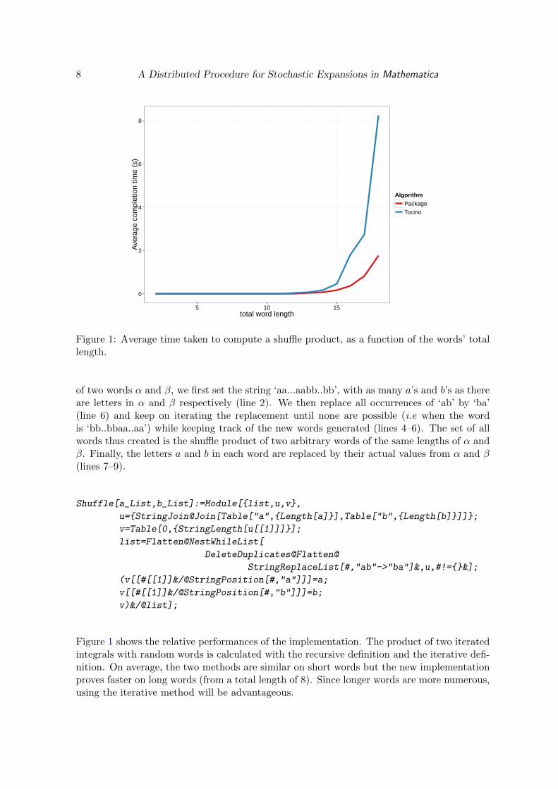
0
2
4
6
8
5 10 15total word length
Ave
rage
com
plet
ion
time
(s)
AlgorithmPackageTocino
Figure 1: Average time taken to compute a shuffle product, as a function of the words’ totallength.
of two words α and β, we first set the string ‘aa...aabb..bb’, with as many a’s and b’s as thereare letters in α and β respectively (line 2). We then replace all occurrences of ‘ab’ by ‘ba’(line 6) and keep on iterating the replacement until none are possible (i.e when the wordis ‘bb..bbaa..aa’) while keeping track of the new words generated (lines 4–6). The set of allwords thus created is the shuffle product of two arbitrary words of the same lengths of α andβ. Finally, the letters a and b in each word are replaced by their actual values from α and β(lines 7–9).
Shuffle[a_List,b_List]:=Module[{list,u,v},
u={StringJoin@Join[Table["a",{Length[a]}],Table["b",{Length[b]}]]};
v=Table[0,{StringLength[u[[1]]]}];
list=Flatten@NestWhileList[
DeleteDuplicates@Flatten@
StringReplaceList[#,"ab"->"ba"]&,u,#!={}&];
(v[[#[[1]]&/@StringPosition[#,"a"]]]=a;
v[[#[[1]]&/@StringPosition[#,"b"]]]=b;
v)&/@list];
Figure 1 shows the relative performances of the implementation. The product of two iteratedintegrals with random words is calculated with the recursive definition and the iterative defi-nition. On average, the two methods are similar on short words but the new implementationproves faster on long words (from a total length of 8). Since longer words are more numerous,using the iterative method will be advantageous.
Journal of Statistical Software 9
3.2. Non-commutative product
The non-commutative and non-associative product B is implemented as � in Mathematica,an operation with no built-in meaning. We only set a few basic properties for this product:
Unprotect[CircleDot]; (* $\odot$ = esc c . esc *)
1$\odot$x_ := x;
x_$\odot$1 := 0;
0$\odot$x_ := 0;
x_$\odot$0 := 0;
Protect[CircleDot];
Since � is only used as a placeholder, its actual definition in terms of shuffle product (Equa-tion 10) is coded in another function, NCP:
NCP[0, j[b_List]] := 0;
NCP[1, j[b_List]] := j[b];
NCP[j[a_List], 0] := 0;
NCP[j[a_List], 1] := j[a];
NCP[j[a_List], j[{}]] := j[a];
NCP[j[a_List], j[b_List]] :=
Ap[j[a]*j[Drop[b, -1]], Last[b]] /; Length[b] > 0;
NCP[n_*j[a_List], j[b_List]] := n*NCP[j[a], j[b]];
NCP[j[a_List], n_*j[b_List]] := n*NCP[j[a], j[b]];
NCP[n_*j[a_List], m_*j[b_List]] := n*m*NCP[j[a], j[b]];
NCP[x_ + y_, z_] := NCP[x, z] + NCP[y, z];
NCP[x_, y_ + z_] := NCP[x, y] + NCP[x, z];
NCP[x_*(y_ + z_), t_] := NCP[x*y, t] + NCP[x*z, t];
NCP[(y_ + z_)*x_, t_] := NCP[x*y, t] + NCP[x*z, t];
3.3. Picard iteration
The usual Picard iteration is implemented with a helper function PicardIteration as fol-lowing:
PicardIteration[f_List,X_]:=
Total[MapIndexed[(Ap[#1[X]*j[{}],First[#2]-1])&,f]]
Picard[f_List,X0_,n_Integer]:=
Nest[(PicardIteration[f,#])&,X0,n]
For example, Picard[f,x0,4] outputs the stochastic approximation of the SDE with thefunctions f collected in a list in the first argument. This was used in Papavasiliou andLadroue (2010) for a system with linear drift and quadratic variance.
With the new representation in Q, it can be written directly as in Equation 2:
PicardQ1Dim[Q_, R_, q_] :=
Nest[Q[0] + Sum[(#^r)$\odot$Q[r], {r, 1, q}] &, Q[0], R - 1];
10 A Distributed Procedure for Stochastic Expansions in Mathematica
R is the number of iterations to be calculated and q the maximum degree of the polynomialsf . PicardQ1Dim[] produces a very compact representation of the expansion, which needs tobe processed further in order to give the same result as Picard[].
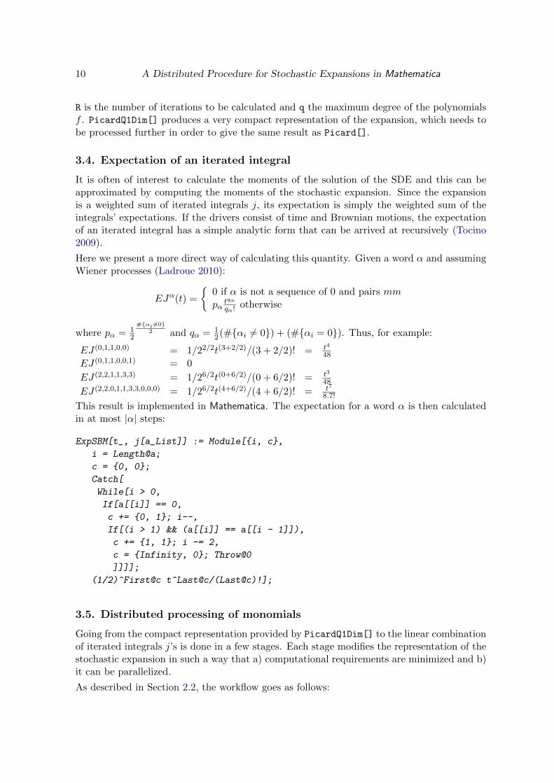
3.4. Expectation of an iterated integral
It is often of interest to calculate the moments of the solution of the SDE and this can beapproximated by computing the moments of the stochastic expansion. Since the expansionis a weighted sum of iterated integrals j, its expectation is simply the weighted sum of theintegrals’ expectations. If the drivers consist of time and Brownian motions, the expectationof an iterated integral has a simple analytic form that can be arrived at recursively (Tocino2009).
Here we present a more direct way of calculating this quantity. Given a word α and assumingWiener processes (Ladroue 2010):
EJα(t) =
{0 if α is not a sequence of 0 and pairs mm
pαtqαqα!
otherwise
where pα = 12
#{αi 6=0}2 and qα = 1
2(#{αi 6= 0}) + (#{αi = 0}). Thus, for example:
EJ (0,1,1,0,0) = 1/22/2t(3+2/2)/(3 + 2/2)! = t4
48
EJ (0,1,1,0,0,1) = 0
EJ (2,2,1,1,3,3) = 1/26/2t(0+6/2)/(0 + 6/2)! = t3
48
EJ (2,2,0,1,1,3,3,0,0,0) = 1/26/2t(4+6/2)/(4 + 6/2)! = t7
8.7!
This result is implemented in Mathematica. The expectation for a word α is then calculatedin at most |α| steps:
ExpSBM[t_, j[a_List]] := Module[{i, c},
i = Length@a;
c = {0, 0};
Catch[
While[i > 0,
If[a[[i]] == 0,
c += {0, 1}; i--,
If[(i > 1) && (a[[i]] == a[[i - 1]]),
c += {1, 1}; i -= 2,
c = {Infinity, 0}; Throw@0
]]]];
(1/2)^First@c t^Last@c/(Last@c)!];
3.5. Distributed processing of monomials
Going from the compact representation provided by PicardQ1Dim[] to the linear combinationof iterated integrals j’s is done in a few stages. Each stage modifies the representation of thestochastic expansion in such a way that a) computational requirements are minimized and b)it can be parallelized.
As described in Section 2.2, the workflow goes as follows:
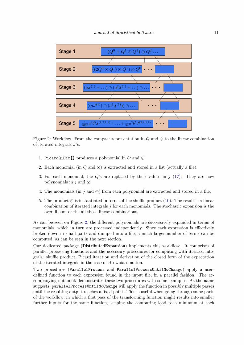
Journal of Statistical Software 11
Stage 1
Stage 2
Stage 3
Stage 4
Stage 5
Figure 2: Workflow. From the compact representation in Q and � to the linear combinationof iterated integrals J ’s.
1. PicardQ1Dim[] produces a polynomial in Q and �.
2. Each monomial (in Q and �) is extracted and stored in a list (actually a file).
3. For each monomial, the Q’s are replaced by their values in j (17). They are nowpolynomials in j and �.
4. The monomials (in j and �) from each polynomial are extracted and stored in a file.
5. The product � is instantiated in terms of the shuffle product (10). The result is a linearcombination of iterated integrals j for each monomials. The stochastic expansion is theoverall sum of the all those linear combinations.
As can be seen on Figure 2, the different polynomials are successively expanded in terms ofmonomials, which in turn are processed independently. Since each expression is effectivelybroken down in small parts and dumped into a file, a much larger number of terms can becomputed, as can be seen in the next section.
Our dedicated package (DistributedExpansion) implements this workflow. It comprises ofparallel processing functions and the necessary procedures for computing with iterated inte-grals: shuffle product, Picard iteration and derivation of the closed form of the expectationof the iterated integrals in the case of Brownian motion.
Two procedures (ParallelProcess and ParallelProcessUntilNoChange) apply a user-defined function to each expression found in the input file, in a parallel fashion. The ac-companying notebook demonstrates these two procedures with some examples. As the namesuggests, parallelProcessUntilNoChange will apply the function in possibly multiple passesuntil the resulting output reaches a fixed point. This is useful when going through some partsof the workflow, in which a first pass of the transforming function might results into smallerfurther inputs for the same function, keeping the computing load to a minimum at each
12 A Distributed Procedure for Stochastic Expansions in Mathematica
step. The procedures require the creation of temporary files, one per processor, to avoid theconcurrent overwriting of the output file.
In the following example, an input file is created that contains 2000 random integers. Eachinteger is factorized in parallel. A simple test then checks that the factorization is correct.The order of the inputs does not necessarily match that of the outputs, owing to the parallelcalls to the input file and the varying processing time of each factorization.
original=Table[Random[Integer,10^3],{2000}];
in=OpenWrite@"buffer/seed";
Scan[PutAppend[#,in]&,original];
Close@in;
ParallelProcess["buffer/seed","buffer/result",FactorInteger];
in=OpenRead@"buffer/result";after=ReadList[in];Close@in;
rebuild[x_]:=Fold[#1*(#2[[1]]^#2[[2]])&,1,x];
If[Fold[Times,1,original]!=rebuild@after,
Print@"Total products are different!",
Print@"It's working"]
Thanks to the parallel processing functions, the workflow is implemented very easily, by defin-ing one function per stage. The whole method is written in the procedureParallelStochasticExpansion, so the stochastic expansion of a SDE can be calculatedin one call to this function.
4. Example
Consider the following SDE: dYt = a(1− Yt)dX1 + bY 2t dX2 and Y0 = 0. In this case, m = 1,
n = 2, q = 2. The two functions f are f1,1(x) = a(1− x) and f1,2(x) = bx2.
Only two things are required from the user: the definition of the objects Q in a transformationrule, easily obtained by derivation (17), and the number of Picard iterations to be computed.In this case, the three Q’s are:
Q0 =1
0!(a(1− 0)X(1 + b02X(2))
= aX(1)
Q1 =1
1!(−aX(1) + 2b0X(2))
= −aX(1)
Q2 =1
2!(0X(1 + 2bX(2))
= bX(2)
Therefore, the transformation rule corresponding to this system is:
ruleModel={Q[0]->aj[{1}],Q[1]->-aj[{1}],Q[2]->bj[{2}]}};
If the first driver is time, we can follow the convention that drivers are numbered from 0:
Journal of Statistical Software 13
2 3 4 5 6 7 8Processors
1600
1700
1800
1900
2000
2100
2200
Completetion time H s L
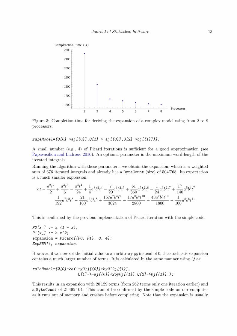
Figure 3: Completion time for deriving the expansion of a complex model using from 2 to 8processors.
ruleModel={Q[0]->aj[{0}],Q[1]->-aj[{0}],Q[2]->bj[{1}]}};
A small number (e.g., 4) of Picard iterations is sufficient for a good approximation (seePapavasiliou and Ladroue 2010). An optional parameter is the maximum word length of theiterated integrals.
Running the algorithm with these parameters, we obtain the expansion, which is a weightedsum of 676 iterated integrals and already has a ByteCount (size) of 504’768. Its expectationis a much smaller expression:
at− a2t2
2+a3t3
6− a4t4
24+
1
4a3b2t4 − 7
20a4b2t5 +
61
360a5b2t6 − 1
24a6b2t7 +
17
140a5b4t7
1
192a7b2t8 − 21
160a6b4t8 +
157a7b4t9
3024− 17a8b4t10
2800+
43a7b6t10
1800− 1
100a8b6t11
This is confirmed by the previous implementation of Picard iteration with the simple code:
P0[x_] := a (1 - x);
P1[x_] := b x^2;
expansion = Picard[{P0, P1}, 0, 4];
ExpSBM[t, expansion]
However, if we now set the initial value to an arbitrary y0 instead of 0, the stochastic expansioncontains a much larger number of terms. It is calculated in the same manner using Q as:
ruleModel={Q[0]->a(1-y0)j[{0}]+by0^2j[{1}],
Q[1]->-aj[{0}]+2by0j[{1}],Q[2]->bj[{1}] };
This results in an expansion with 20 129 terms (from 262 terms only one iteration earlier) anda ByteCount of 21 495 104. This cannot be confirmed by the simple code on our computeras it runs out of memory and crashes before completing. Note that the expansion is usually
14 A Distributed Procedure for Stochastic Expansions in Mathematica
left in a file whose entries are parts of the linear combination. Thus, it is possible to, forexample, compute the expectation of the expansion without having to store it in memory atany point. Moreover, while computationally expensive, these expansions can be calculatedonce in a general case and saved in a file for future application without having to recomputethem de novo.
The notebook DistributedExpansion.nb provides a few examples and validations of theapproach.
Figure 3 shows how the performance changes with the number of processors used. There isan increase in speed until the performance reaches a plateau. This is due to an input/outputbottleneck which takes a constant time (the collection of expression’ positions in a file, to beassigned to the different processors).
5. Conclusion
Stochastic expansions provide a local approximation of the solution of a stochastic (or deter-ministic) differential equation. They can be used for a variety of applications, from simulationto parameter estimation. However, as the number of terms grows exponentially with the de-sired precision, they can rapidly become unwieldy to manipulate.
We presented a new way of calculating these expansions that bypasses the limitation of theusual approach, via a reparametrization of the problem and the parallelization of the computa-tion. We have shown that in a simple example our method was able to compute the expansionwhen a direct approach failed. We also presented two new approaches for efficiently derivingthe shuffle product of two iterated integrals and the expectation of an iterated integral, whenthe drivers are time and Brownian motion.
So far, our approach has been implemented for one-dimensional differential equation. How-ever, the theoretical foundation for the multi-dimensional case is available, as presented inSection 2.3. Now that the computing requirements have been alleviated, an implementationfor the general case is possible. Stochastic expansions will then be available for more complexsystems.
Acknowledgments
This work was funded by the EPSRC (EP/H019588/1, ‘Parameter Estimation for RoughDifferential Equations with Applications to Multiscale Modelling’). We would like to thankthe Mathematica newsgroup (comp.soft-sys.math.mathematica group) for their help andadvice on file parallelization. We are also grateful to the reviewer for their suggestions andtheir help.
References
Kendall WS (2005). “Stochastic Integrals and Their Expectations.”The Mathematica Journal,9(4).
Journal of Statistical Software 15
Kloeden PE, Platen E (1991). “Relations between Multiple Ito and Stratonovich Integrals.”Stochastic Analysis and Applications, 9(3), 311–321.
Ladroue C (2010). “Expectation of Stratonovich Iterated Integrals of Wiener Processes.”ArXiv:1008.4033 [math.PR], URL http://arxiv.org/abs/1008.4033.
Lyons T, Qian Z (2003). System Control and Rough Paths. Oxford University Press.
Papavasiliou A, Ladroue C (2010). “Parameter Estimation for Rough Differential Equations.”ArXiv:0812.3102 [math.PR], URL http://arxiv.org/abs/0812.3102.
Tocino A (2009). “Multiple Stochastic Integrals with Mathematica.” Mathematics and Com-puters in Simulation, 79(5), 1658–1667.
Wolfram S (2003). The Mathematica Book. 5th edition. Wolfram Media.
Affiliation:
Christophe Ladroue, Anastasia PapavaviliouDepartment of Computer ScienceUniversity of WarwickCV47AL, Coventry, United KingdomE-mail: [email protected], [email protected]: http://www2.warwick.ac.uk/fac/sci/statistics/staff/academic/papavasiliou
Journal of Statistical Software http://www.jstatsoft.org/
published by the American Statistical Association http://www.amstat.org/
Volume 53, Issue 11 Submitted: 2010-08-25May 2013 Accepted: 2013-01-03


![1 Distributed Asynchronous Constrained Stochastic …angelia/tsp_final_single.pdfproblem of cooperative solution to distributed optimization problems [6]–[11]. The algorithms for](https://img.pdfslide.net/doc/110x75/5fdb2976effc1c7fef55fd29/1-distributed-asynchronous-constrained-stochastic-angeliatspfinalsinglepdf-problem.jpg)