Embed Size (px)
Citation preview
A DNS study of turbulent mixing of two passive scalarsA. Junejaa) and S. B. PopeSibley School of Mechanical and Aerospace Engineering, Cornell University, Ithaca, New York 14853
~Received 12 March 1996; accepted 25 April 1996!
We employ direct numerical simulations to study the mixing of two passive scalars in stationary,homogeneous, isotropic turbulence. The present work is a direct extension of that of Eswaran andPope1 from one scalar to two scalars and the focus is on examining the evolution states of the scalarjoint probability density function~jpdf! and the conditional expectation of the scalar diffusion tomotivate better models for multi-scalar mixing. The initial scalar fields are chosen to conformclosely to a ‘‘triple-delta function’’ jpdf corresponding to blobs of fluid in three distinct states. Theeffect of the initial length scales and diffusivity of the scalars on the evolution of the jpdf and theconditional diffusion is investigated in detail as the scalars decay from their prescribed initial state.Also examined is the issue of self-similarity of the scalar jpdf at large times and the rate of decayof the scalar variance and dissipation. ©1996 American Institute of Physics.@S1070-6631~96!03108-X#
I. INTRODUCTION
An important feature of turbulent motion is its ability tomix and to transport passive scalars at rates much higherthan those due to molecular diffusion. Often, more than onescalar is involved in the mixing process. Examples of thiscan readily be seen in natural or engineering flows such asthe dispersion of pollutants in the atmosphere, salinity andtemperature fluctuations in the ocean, and the mixing of spe-cies in turbulent reactive flows. While the turbulence under-lying the above flows is essentially time dependent and in-homogeneous, a detailed study of these complex flows doesnot highlight any one physical concept or mechanism be-cause there are so many interacting processes at work. In-deed, it is of great interest to investigate simple flows whichclearly elucidate the basic mechanisms involved in turbulentmixing without the added complications of inhomogeneity,complex flow geometries or decaying turbulence. Over thelast couple of decades, direct numerical simulations~DNS!of the Navier-Stokes equations have emerged as a leadingresearch tool for examining the physics of turbulence atmoderate Reynolds numbers because of their unique abilityto provide fully resolved spatio-temporal evolution of theflow fields without any modeling or approximations. Conse-quently, the present work employs DNS to study the mixingof two decaying scalar fields with a prescribed initial jointprobability density function~jpdf! in statistically stationary,homogeneous, isotropic turbulence.
A significant amount of experimental and computationaleffort has been exerted to study the mixing of a single pas-sive scalar in turbulent flows. A number of researchers havestudied the evolution of one-point and two-point quantitiesof scalar fields in grid turbulence~see, e.g., Refs. 2 and 3!.Laser Induced Flouresence~LIF! techniques have been usedto obtain and study images of instantaneous scalar fields inturbulent flows4,5 and Dahmet al.6 have developed a methodfor acquiring a sequence of planar LIF images sweeping a
volume to get four-dimensional experimental data on scalarmixing. On the other hand, Eswaran and Pope1 employedDNS to examine the evolution of the probability densityfunction of a single scalar from an initial double-delta func-tion distribution, while Kerr7 used DNS to examine the smallscale structure of the passive scalar. Blaisdellet al.8 havecarried out simulations to assess the effects of compressibil-ity on the mixing process, and Pumir9 has studied the casewith a mean scalar gradient. Chasnov10 also used DNS topresent results for the similarity states of a passive scalarfield transported by isotropic and buoyancy generated turbu-lence. Theoretical approaches which have been applied to themixing of a single scalar with some success include probabil-ity density function~pdf! methods,11 mapping closures12 andthe linear eddy model.13
In contrast, data on the mixing of multiple scalars isrelatively scarce. Sirivat and Warhaft14 measured the corre-lation between passive helium and temperature measure-ments in grid generated turbulence. Warhaft15 also developedan inference technique to study the covariance of thermalfluctuations introduced in decaying turbulence at differentlocations. Yeung and Pope16 employed DNS to examine thedifferential diffusion of two scalars having different diffu-sivities starting from an identical field for the two scalars,while experimental studies of differential diffusion havebeen reported by Saylor17 among others. The extension ofthe theoretical approaches to multi-scalar mixing is far fromstraightforward, and is further hampered by the lack of ex-perimental or numerical data which can aid in model com-parison and development.
Research on turbulent mixing processes is especially in-structive in turbulent-reactive flow problems. Here, in thelimit of fast chemistry, one of the vital factors limiting therate of reaction is the mixing of initially segregated scalarfields at the smallest scales at which the chemical reactiontakes place. Pdf formulations have had considerable successin modeling reactive flow problems.11 These methods havethe important advantage of treating the effects of advectionand the nonlinear reaction rates exactly: however the processof molecular mixing needs to be modeled. We consider non-
a!Present address: Department of Mechanical Engineering, The PennsylvaniaState University, University Park, Pennsylvania 16802.
2161Phys. Fluids 8 (8), August 1996 1070-6631/96/8(8)/2161/24/$10.00 © 1996 American Institute of Physics
Downloaded¬22¬Sep¬2004¬to¬140.121.120.39.¬Redistribution¬subject¬to¬AIP¬license¬or¬copyright,¬see¬http://pof.aip.org/pof/copyright.jsp
reactive scalar fieldsfa(x,t),a51,2, which evolve by
]fa
]t1ui
]fa
]xi5D ~a!¹
2fa , ~1!
whereu(x,t) is the velocity andD (a) is the diffusivity of thescalar a. ~Suffixes in parentheses are excluded from thesummation convention.! For the statistically homogeneouscase under consideration, the one-point one-time joint prob-ability density function~jpdf! of the two scalars is denotedby P(c;t), wherec5(c1 ,c2) are the sample space vari-ables corresponding tof5(f1 ,f2). This jpdf evolves by
11
]P~c;t !
]t52
]
]ca@P~c;t !ga~c,t !#, ~2!
where the conditional diffusiong(c,t) is defined to be theconditional expectation,
ga~c,t !5^D ~a!¹2fauf~x,t !5c&. ~3!
In the present work, we examine the evolution of the scalarjpdf P and the conditional diffusiong for the mixing of twoscalars starting from a prescribed initial state~triple-deltafunction jpdf!. The work is in essence an extension of thatpresented in Eswaran and Pope~hereafter EP! and it is hopedthat the present results will provide the necessary impetus forthe development of better mixing models for the multi-scalarcase.
A parallel implementation of Rogallo’s pseudospectralalgorithm18 for the IBM SP2 is used to carry out direct nu-merical simulations of the governing equations in a cubicdomain with periodic boundary conditions. The low wave-number modes are forced using the scheme described in Es-waran and Pope19 to preserve statistical stationarity in thevelocity fields. The scalar fields are allowed to decay fromtheir prescribed initial state and we examine the evolution ofthe scalar jpdf and the conditional diffusion in detail. The
effect of varying the initial length scales and the Prandtlnumber of the two scalars on the mixing process is investi-gated. Also examined is the tendency of the scalar jpdf toreach a statistically self-similar state at large times as well asthe rate of decay of scalar variance and the mean scalar dis-sipation rate. Nearly all the simulations were carried out on a1923 grid at a Taylor-scale Reynolds number ofRel592,excepting a few requiring the extraction of statistics at largetimes which were performed on a smaller 963 grid at aTaylor-scale Reynolds number ofRel548 in order to keepthe overall computational costs low. This also gave an op-portunity to qualitatively compare the mixing process at dif-ferent Reynolds numbers.
The remainder of the paper is organized as follows. InSec. II we provide a brief overview of the simulations in-cluding the numerical method, parallel implementation andthe input flow conditions. In Sec. III we describe the methodfor initializing the two scalar fields. The results from thesimulations are presented in Sec. IV. We conclude the paperwith a summary in Sec. V.
II. OVERVIEW OF THE SIMULATIONS
A. The numerical method
For incompressible flows, the equations governing theevolution of the velocity and scalar fields can be written as
TABLE I. Summary of specified quantities for initial velocity fields.
Vel. field R92 R48
N 192 96n 0.008 0.025KF 2A2 2A2Re* 14.4 14.4TF* 0.15 0.15CN 0.8 0.8
TABLE II. Summary of derived quantities for initial velocity fields.
Vel. field R92 R48
u 2.06 2.16k0l 1.10 1.05k0l 0.35 0.51k0h 0.02 0.04kmaxh 1.65 1.78D* 0.49 0.49T 0.52 0.50
th /T 0.08 0.14Rel 92.4 48.6
TABLE III. Summary of input parameters for scalar fields.
Scalar field A B C D E
(ks /k0)1 4 8 2 2 4(ks /k0)2 4 8 2 4 4Pr1 0.7 0.7 0.7 0.7 0.7Pr2 0.7 0.7 0.7 0.7 0.35lf1
0.38 0.16 0.62 0.62 0.38lf2
0.37 0.18 0.58 0.40 0.37^f1f2& 20.0006 0.0025 0.001 20.009 20.0006
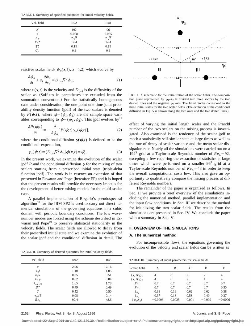
FIG. 1. A schematic for the initialization of the scalar fields. The composi-tion plane represented byc1-c2 is divided into three sectors by the twodashed lines and the negativec2 axis. The filled circles correspond to thethree initial states for the two scalar fields.~The evolution of the conditionaldiffusion in Fig. 5 is shown along the two axes and the two dotted lines.!
2162 Phys. Fluids, Vol. 8, No. 8, August 1996 A. Juneja and S. B. Pope
Downloaded¬22¬Sep¬2004¬to¬140.121.120.39.¬Redistribution¬subject¬to¬AIP¬license¬or¬copyright,¬see¬http://pof.aip.org/pof/copyright.jsp
]ui]xi
50, ~4!
]ui]t
1uj]ui]xj
521
r
]p
]xi1n
]2ui]xj]xj
, ~5!
]fa
]t1uj
]fa
]xj5D ~a!
]2fa
]xj]xj, ~6!
whereui is the component of the velocity in thei th direction.A modified version of the pseudo-spectral method developed
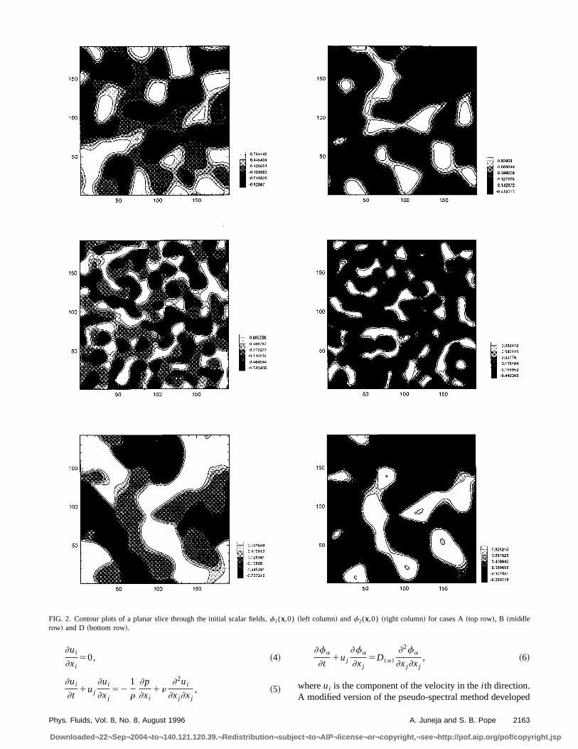
FIG. 2. Contour plots of a planar slice through the initial scalar fields,f1(x,0) ~left column! andf2(x,0) ~right column! for cases A~top row!, B ~middlerow! and D ~bottom row!.
2163Phys. Fluids, Vol. 8, No. 8, August 1996 A. Juneja and S. B. Pope
Downloaded¬22¬Sep¬2004¬to¬140.121.120.39.¬Redistribution¬subject¬to¬AIP¬license¬or¬copyright,¬see¬http://pof.aip.org/pof/copyright.jsp
by Rogallo18 for homogeneous turbulent flows was used tosolve the above equations numerically on a uniform three-dimensional grid. In physical space, this corresponds to acube of sideL52p with the N3 grid points located atx5( l 1D,l 2D,l 3D), wherel 1 , l 2 and l 3 are integers between0 andN21 and the grid spacingD is equal toL/N. Thenodes in wavenumber space are located atk5(m1 ,m2 ,m3)wherem1 , m2 and m3 are integers between 12N/2 andN/2. ~The smallest wavenumber isk051 owing toL beingequal to 2p.) The use of Fourier representation imposesperiodic boundary conditions on the velocity and scalarfields.
Briefly, the pseudo-spectral method solves the aboveequations in spectral space because of the associated higheraccuracy in computing the spatial derivatives. However, thebilinear products required for the convective terms are com-puted in physical space to avoid the costly operation of con-volutions in Fourier space. The aliasing errors introduced bythe transformation of these products back to Fourier spaceare greatly reduced by a combination of phase shifts andtruncation. The viscous terms are treated exactly and are thuseliminated as a stability constraint. The time advance of theFourier transformed equations is performed using an explicitsecond-order Runge-Kutta method.
The numerical simulations are forced using the methoddescribed in Eswaran and Pope.19 It consists of the additionof a random term to the velocity time derivative in Fourierspace, at every time step, for each non-zero wavenumbernodek lying within the spherical shell of radiusKF . Therandom term is determined using a combination of indepen-dent Uhlenbeck-Ornstein processes. The forcing scheme in-troduces three nondimensional quantities in the form of aforcing Reynolds numberRe* , a forcing time scaleT* andthe ratioKF /k0 ~see Ref. 19 for details!. Each of these pa-rameters is kept constant for all the simulations presentedherein.
Numerical accuracy depends on both the spatial and thetemporal resolution. The former requires that the smallestdynamically significant scales of motion characterized by theKolmogorov length scaleh be well resolved by the physicalgrid. It is customary to characterize the spatial resolution of asimulation by the dimensionless parameterkmaxh wherekmax is the highest resolvable wavenumber of the simulation.It has been suggested that a value ofkmaxh51.0 is adequatefor low-order velocity statistics, but a value of at least 1.5 isneeded for higher-order quantities such as the dissipation andderivative statistics.20 In order to determine the resolutionrequirements for the evolution of the scalar field, we carriedout test simulations with one passive scalar~Prandtl number,Pr50.7) on 643, 963 and 1283 grids at a Taylor-scale Rey-nolds number ofRel550 corresponding tokmaxh being ap-proximately equal to 1.1, 1.6 and 2.2, respectively. It wasfound that the evolution of̂¹2f& and^¹4f& was very simi-lar for the two finer grids in contrast to the coarser grid.Hence we concluded thatkmaxh>1.5 provides sufficientresolution for the accurate calculation of higher-order scalarstatistics as well. The accuracy of the time integration, on theother hand, is determined by the Courant number defined asCN5( i51
3 (uui u/D)maxDt, whereDt is the size of the timestep. The Courant number was kept constant at a value ofCN50.8 in our simulations in accordance with earliersuggestions19 that it should be less than one for time steppingerrors to be negligibly small.
B. Parallel implementation
The simulations were carried out on the 512-node IBMSP2 at the Cornell Theory Center. The programming modelemployed was the single-program multiple data~SPMD! ap-proach where the same version of the program runs on allnodes. However, the work arrays are distributed across pro-cessors so that each node performs the same operation on its
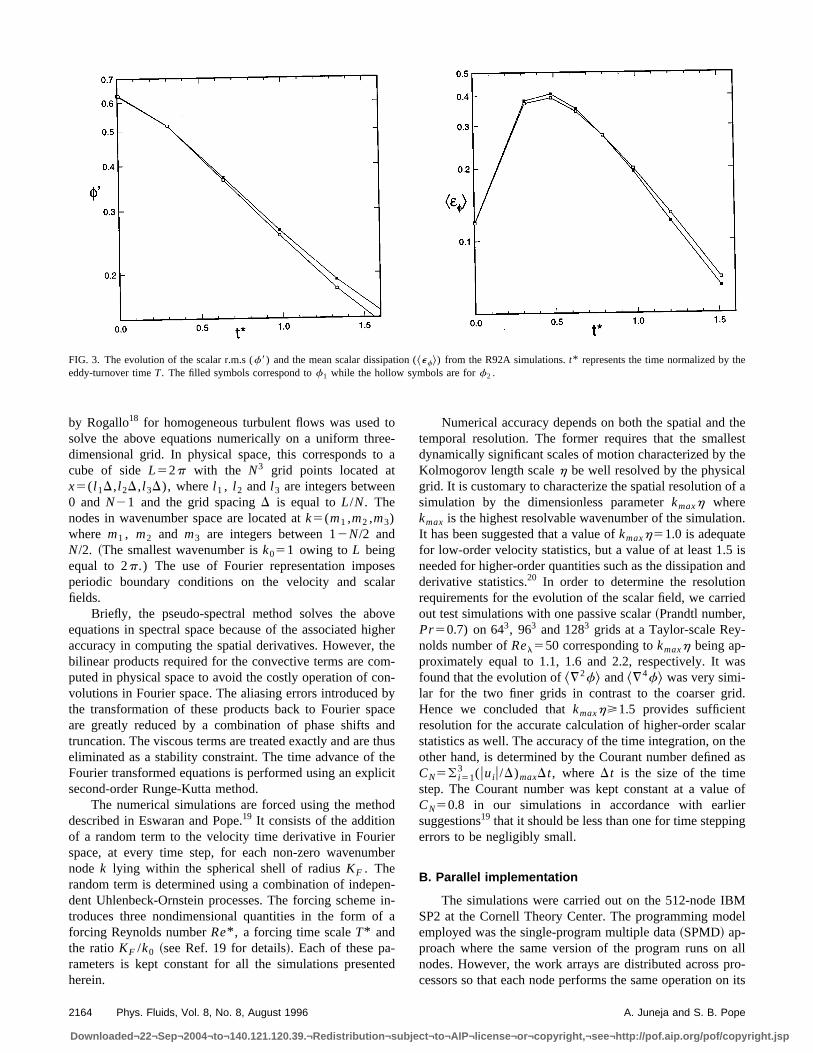
FIG. 3. The evolution of the scalar r.m.s (f8) and the mean scalar dissipation (^ef&) from the R92A simulations.t* represents the time normalized by theeddy-turnover timeT. The filled symbols correspond tof1 while the hollow symbols are forf2 .
2164 Phys. Fluids, Vol. 8, No. 8, August 1996 A. Juneja and S. B. Pope
Downloaded¬22¬Sep¬2004¬to¬140.121.120.39.¬Redistribution¬subject¬to¬AIP¬license¬or¬copyright,¬see¬http://pof.aip.org/pof/copyright.jsp
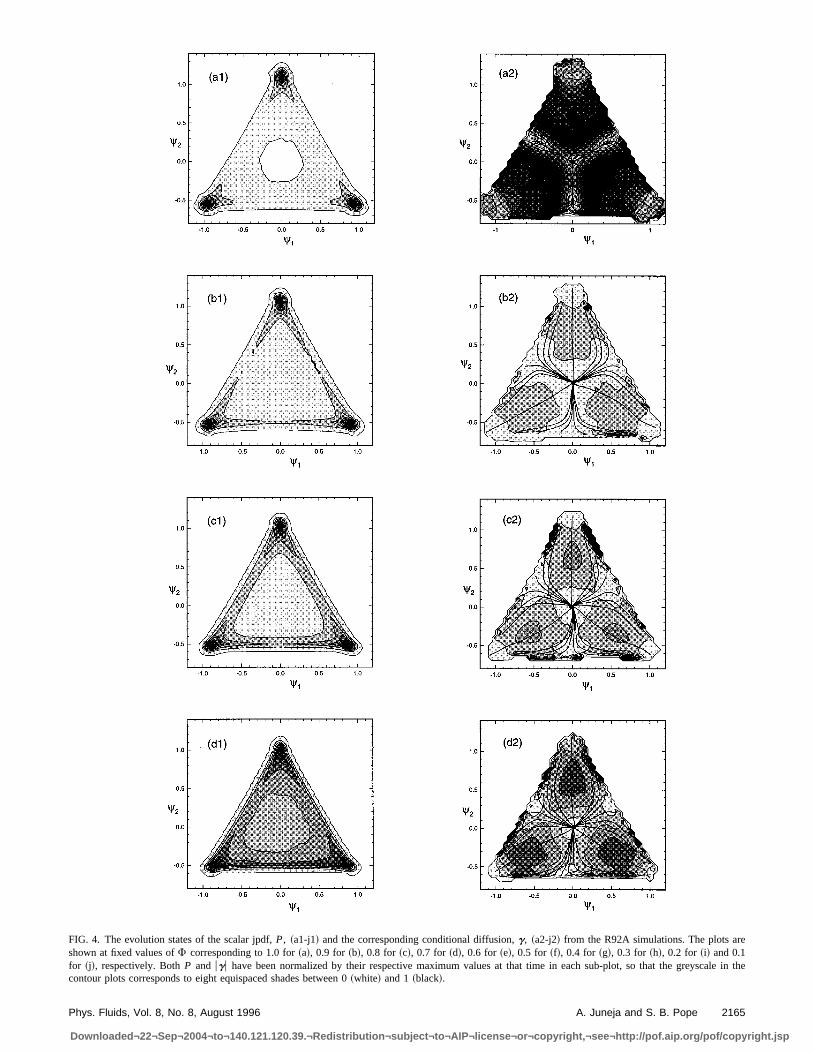
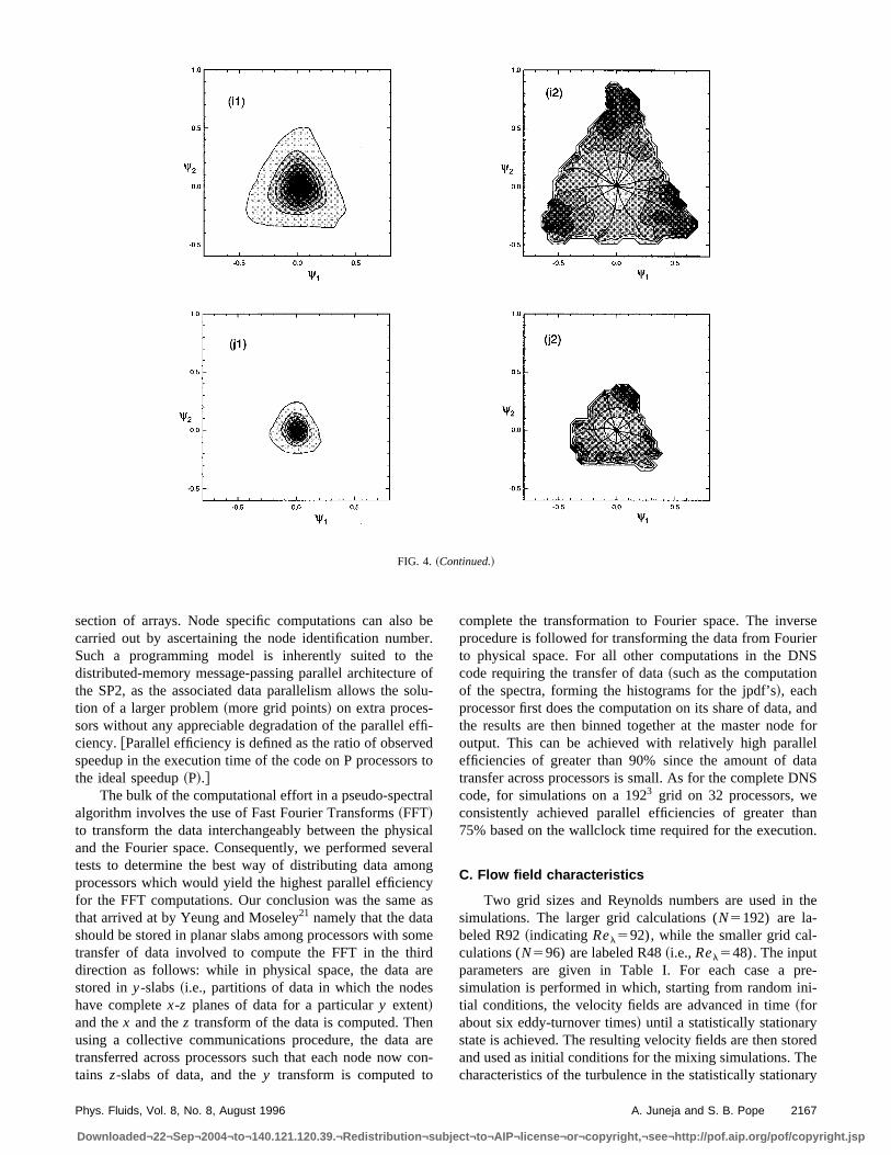
FIG. 4. The evolution states of the scalar jpdf,P, ~a1-j1! and the corresponding conditional diffusion,g, ~a2-j2! from the R92A simulations. The plots areshown at fixed values ofF corresponding to 1.0 for~a!, 0.9 for ~b!, 0.8 for ~c!, 0.7 for ~d!, 0.6 for ~e!, 0.5 for ~f!, 0.4 for ~g!, 0.3 for ~h!, 0.2 for ~i! and 0.1for ~j!, respectively. BothP and ugu have been normalized by their respective maximum values at that time in each sub-plot, so that the greyscale in thecontour plots corresponds to eight equispaced shades between 0~white! and 1~black!.
2165Phys. Fluids, Vol. 8, No. 8, August 1996 A. Juneja and S. B. Pope
Downloaded¬22¬Sep¬2004¬to¬140.121.120.39.¬Redistribution¬subject¬to¬AIP¬license¬or¬copyright,¬see¬http://pof.aip.org/pof/copyright.jsp
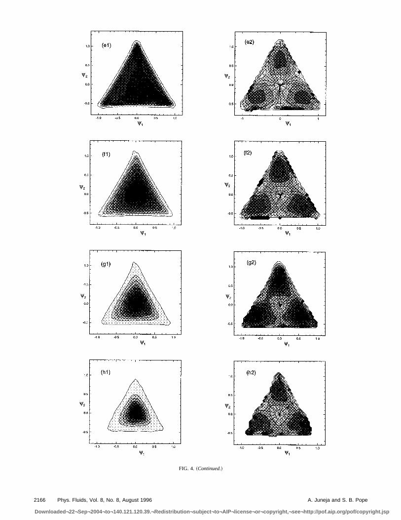
FIG. 4. ~Continued.!
2166 Phys. Fluids, Vol. 8, No. 8, August 1996 A. Juneja and S. B. Pope
Downloaded¬22¬Sep¬2004¬to¬140.121.120.39.¬Redistribution¬subject¬to¬AIP¬license¬or¬copyright,¬see¬http://pof.aip.org/pof/copyright.jsp
section of arrays. Node specific computations can also becarried out by ascertaining the node identification number.Such a programming model is inherently suited to thedistributed-memory message-passing parallel architecture ofthe SP2, as the associated data parallelism allows the solu-tion of a larger problem~more grid points! on extra proces-sors without any appreciable degradation of the parallel effi-ciency.@Parallel efficiency is defined as the ratio of observedspeedup in the execution time of the code on P processors tothe ideal speedup~P!.#
The bulk of the computational effort in a pseudo-spectralalgorithm involves the use of Fast Fourier Transforms~FFT!to transform the data interchangeably between the physicaland the Fourier space. Consequently, we performed severaltests to determine the best way of distributing data amongprocessors which would yield the highest parallel efficiencyfor the FFT computations. Our conclusion was the same asthat arrived at by Yeung and Moseley21 namely that the datashould be stored in planar slabs among processors with sometransfer of data involved to compute the FFT in the thirddirection as follows: while in physical space, the data arestored iny-slabs~i.e., partitions of data in which the nodeshave completex-z planes of data for a particulary extent!and thex and thez transform of the data is computed. Thenusing a collective communications procedure, the data aretransferred across processors such that each node now con-tains z-slabs of data, and they transform is computed to
complete the transformation to Fourier space. The inverseprocedure is followed for transforming the data from Fourierto physical space. For all other computations in the DNScode requiring the transfer of data~such as the computationof the spectra, forming the histograms for the jpdf’s!, eachprocessor first does the computation on its share of data, andthe results are then binned together at the master node foroutput. This can be achieved with relatively high parallelefficiencies of greater than 90% since the amount of datatransfer across processors is small. As for the complete DNScode, for simulations on a 1923 grid on 32 processors, weconsistently achieved parallel efficiencies of greater than75% based on the wallclock time required for the execution.
C. Flow field characteristics
Two grid sizes and Reynolds numbers are used in thesimulations. The larger grid calculations (N5192) are la-beled R92~indicatingRel592), while the smaller grid cal-culations (N596) are labeled R48~i.e.,Rel548). The inputparameters are given in Table I. For each case a pre-simulation is performed in which, starting from random ini-tial conditions, the velocity fields are advanced in time~forabout six eddy-turnover times! until a statistically stationarystate is achieved. The resulting velocity fields are then storedand used as initial conditions for the mixing simulations. Thecharacteristics of the turbulence in the statistically stationary
FIG. 4. ~Continued.!
2167Phys. Fluids, Vol. 8, No. 8, August 1996 A. Juneja and S. B. Pope
Downloaded¬22¬Sep¬2004¬to¬140.121.120.39.¬Redistribution¬subject¬to¬AIP¬license¬or¬copyright,¬see¬http://pof.aip.org/pof/copyright.jsp
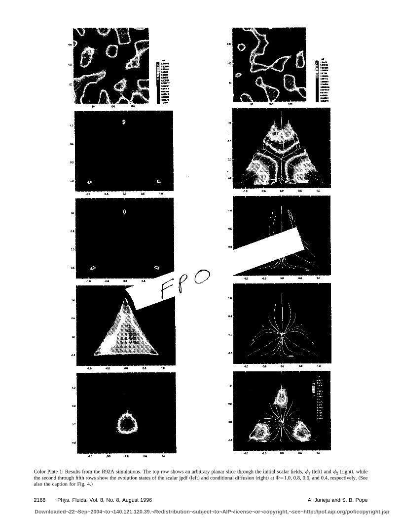
Color Plate 1: Results from the R92A simulations. The top row shows an arbitrary planar slice through the initial scalar fields,f1 ~left! andf2 ~right!, whilethe second through fifth rows show the evolution states of the scalar jpdf~left! and conditional diffusion~right! atF51.0, 0.8, 0.6, and 0.4, respectively.~Seealso the caption for Fig. 4.!
2168 Phys. Fluids, Vol. 8, No. 8, August 1996 A. Juneja and S. B. Pope
Downloaded¬22¬Sep¬2004¬to¬140.121.120.39.¬Redistribution¬subject¬to¬AIP¬license¬or¬copyright,¬see¬http://pof.aip.org/pof/copyright.jsp
state are given in Table II. The root mean square velocity~averaged over the three components! is denoted byu. Thethree length scales characterizing the energy-containingscales, the dissipation scales and the mixed energy-dissipation scales, respectively, are the integral scale,
l5p
2u2E0kmax
k21E~k!dk; ~7!
the Kolmogorov microscale,
h5~n3/e!1/4; ~8!
and the Taylor microscale,
l51
3(i51
3 F u~ i !2
^~]u~ i ! /]x~ i !!2&
G1/2, ~9!
whereE(k) is the energy spectrum function at scalar wave-numberk5(k•k)1/2, and e is the volume averaged energydissipation rate andD* is its non-dimensionalized value(D*[e/u3k0). The time scale of the energy-containing ed-dies is the eddy-turnover timeT5 l /u and the time scale ofthe dissipation range eddies is the Kolmogorov timescaleth5(n/e)1/2. The Reynolds number characterizing the simu-lations isRel5ul/n.
III. INITIAL SCALAR FIELDS
Eswaran and Pope1 studied the mixing of a single scalar(f1) with an initial ~approximate! double-delta-function pdfcorresponding to blobs of fluid in two distinct states,f1'21 andf1'1. Here we extend these ideas to study themixing of two scalars with an initial~approximate! triple-
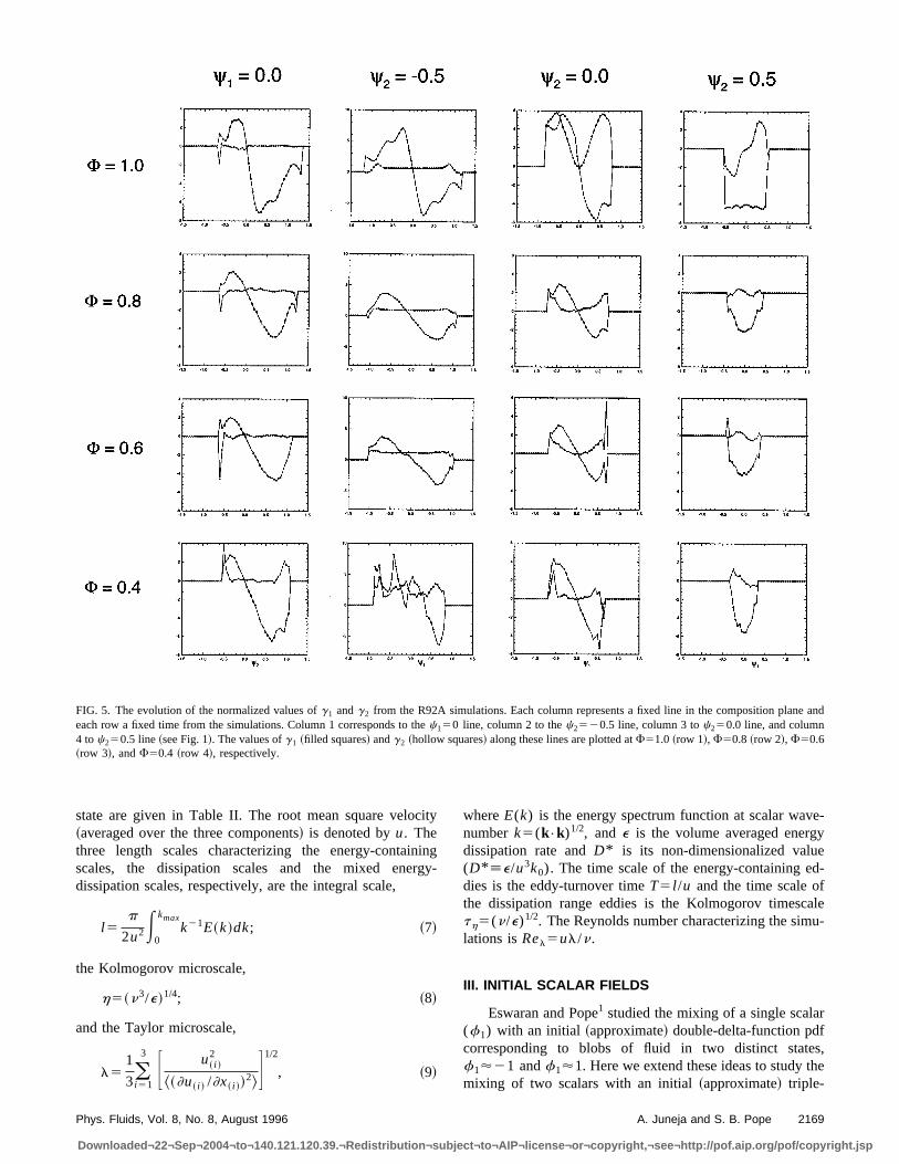
FIG. 5. The evolution of the normalized values ofg1 andg2 from the R92A simulations. Each column represents a fixed line in the composition plane andeach row a fixed time from the simulations. Column 1 corresponds to thec150 line, column 2 to thec2520.5 line, column 3 toc250.0 line, and column4 toc250.5 line~see Fig. 1!. The values ofg1 ~filled squares! andg2 ~hollow squares! along these lines are plotted atF51.0 ~row 1!, F50.8 ~row 2!, F50.6~row 3!, andF50.4 ~row 4!, respectively.
2169Phys. Fluids, Vol. 8, No. 8, August 1996 A. Juneja and S. B. Pope
Downloaded¬22¬Sep¬2004¬to¬140.121.120.39.¬Redistribution¬subject¬to¬AIP¬license¬or¬copyright,¬see¬http://pof.aip.org/pof/copyright.jsp
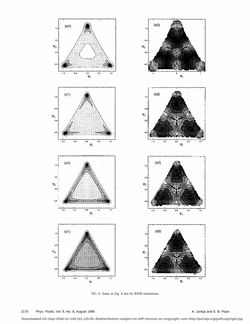
FIG. 6. Same as Fig. 4, but for R92B simulations.
2170 Phys. Fluids, Vol. 8, No. 8, August 1996 A. Juneja and S. B. Pope
Downloaded¬22¬Sep¬2004¬to¬140.121.120.39.¬Redistribution¬subject¬to¬AIP¬license¬or¬copyright,¬see¬http://pof.aip.org/pof/copyright.jsp
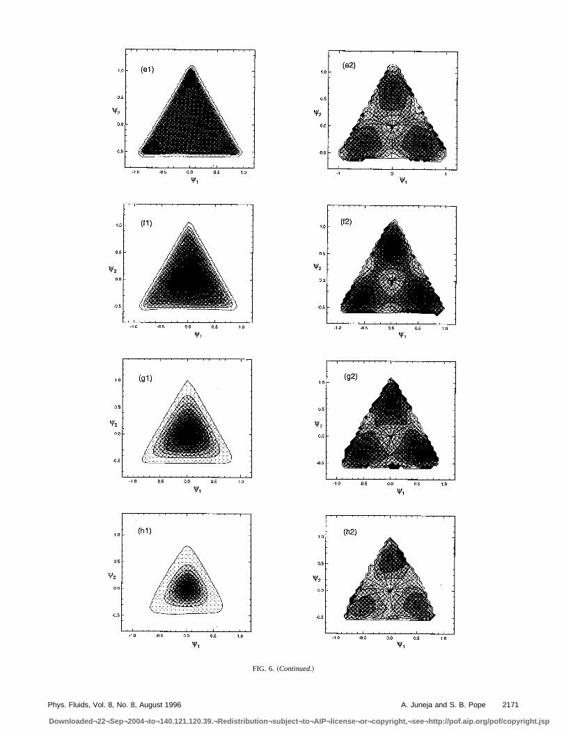
FIG. 6. ~Continued.!
2171Phys. Fluids, Vol. 8, No. 8, August 1996 A. Juneja and S. B. Pope
Downloaded¬22¬Sep¬2004¬to¬140.121.120.39.¬Redistribution¬subject¬to¬AIP¬license¬or¬copyright,¬see¬http://pof.aip.org/pof/copyright.jsp
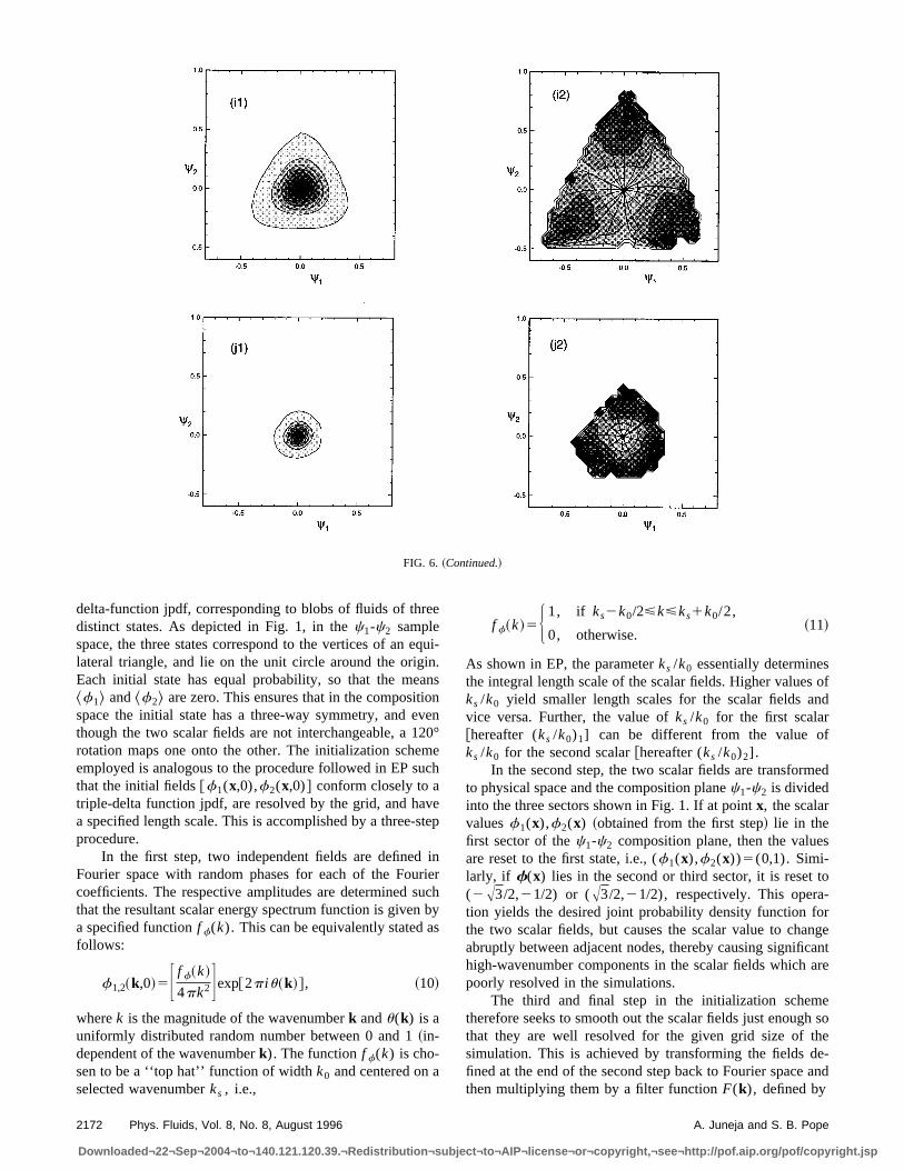
delta-function jpdf, corresponding to blobs of fluids of threedistinct states. As depicted in Fig. 1, in thec1-c2 samplespace, the three states correspond to the vertices of an equi-lateral triangle, and lie on the unit circle around the origin.Each initial state has equal probability, so that the means^f1& and^f2& are zero. This ensures that in the compositionspace the initial state has a three-way symmetry, and eventhough the two scalar fields are not interchangeable, a 120°rotation maps one onto the other. The initialization schemeemployed is analogous to the procedure followed in EP suchthat the initial fields@f1(x,0),f2(x,0)# conform closely to atriple-delta function jpdf, are resolved by the grid, and havea specified length scale. This is accomplished by a three-stepprocedure.
In the first step, two independent fields are defined inFourier space with random phases for each of the Fouriercoefficients. The respective amplitudes are determined suchthat the resultant scalar energy spectrum function is given bya specified functionf f(k). This can be equivalently stated asfollows:
f1,2~k,0!5F f f~k!
4pk2Gexp@2p iu~k!#, ~10!
wherek is the magnitude of the wavenumberk andu(k) is auniformly distributed random number between 0 and 1~in-dependent of the wavenumberk). The functionf f(k) is cho-sen to be a ‘‘top hat’’ function of widthk0 and centered on aselected wavenumberks , i.e.,
ff~k!5H 1, if ks2k0/2<k<ks1k0/2,
0, otherwise.~11!
As shown in EP, the parameterks /k0 essentially determinesthe integral length scale of the scalar fields. Higher values ofks /k0 yield smaller length scales for the scalar fields andvice versa. Further, the value ofks /k0 for the first scalar@hereafter (ks /k0)1] can be different from the value ofks /k0 for the second scalar@hereafter (ks /k0)2].
In the second step, the two scalar fields are transformedto physical space and the composition planec1-c2 is dividedinto the three sectors shown in Fig. 1. If at pointx, the scalarvaluesf1(x),f2(x) ~obtained from the first step! lie in thefirst sector of thec1-c2 composition plane, then the valuesare reset to the first state, i.e., (f1(x),f2(x))5(0,1). Simi-larly, if f(x) lies in the second or third sector, it is reset to(2A3/2,21/2) or (A3/2,21/2), respectively. This opera-tion yields the desired joint probability density function forthe two scalar fields, but causes the scalar value to changeabruptly between adjacent nodes, thereby causing significanthigh-wavenumber components in the scalar fields which arepoorly resolved in the simulations.
The third and final step in the initialization schemetherefore seeks to smooth out the scalar fields just enough sothat they are well resolved for the given grid size of thesimulation. This is achieved by transforming the fields de-fined at the end of the second step back to Fourier space andthen multiplying them by a filter functionF(k), defined by
FIG. 6. ~Continued.!
2172 Phys. Fluids, Vol. 8, No. 8, August 1996 A. Juneja and S. B. Pope
Downloaded¬22¬Sep¬2004¬to¬140.121.120.39.¬Redistribution¬subject¬to¬AIP¬license¬or¬copyright,¬see¬http://pof.aip.org/pof/copyright.jsp
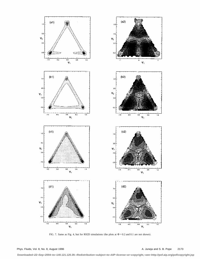
FIG. 7. Same as Fig. 4, but for R92D simulations~the plots atF50.2 and 0.1 are not shown!.
2173Phys. Fluids, Vol. 8, No. 8, August 1996 A. Juneja and S. B. Pope
Downloaded¬22¬Sep¬2004¬to¬140.121.120.39.¬Redistribution¬subject¬to¬AIP¬license¬or¬copyright,¬see¬http://pof.aip.org/pof/copyright.jsp
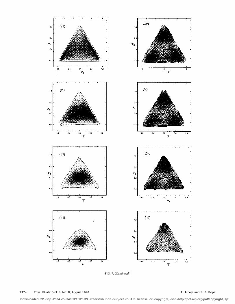
FIG. 7. ~Continued.!
2174 Phys. Fluids, Vol. 8, No. 8, August 1996 A. Juneja and S. B. Pope
Downloaded¬22¬Sep¬2004¬to¬140.121.120.39.¬Redistribution¬subject¬to¬AIP¬license¬or¬copyright,¬see¬http://pof.aip.org/pof/copyright.jsp
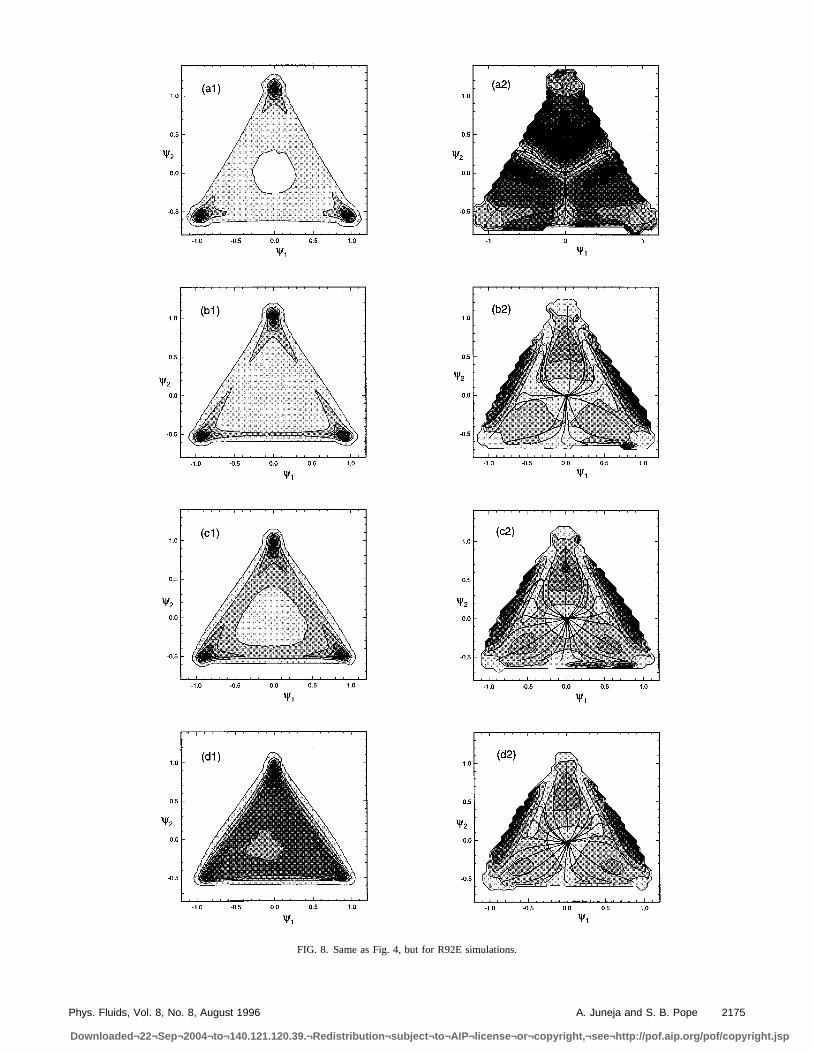
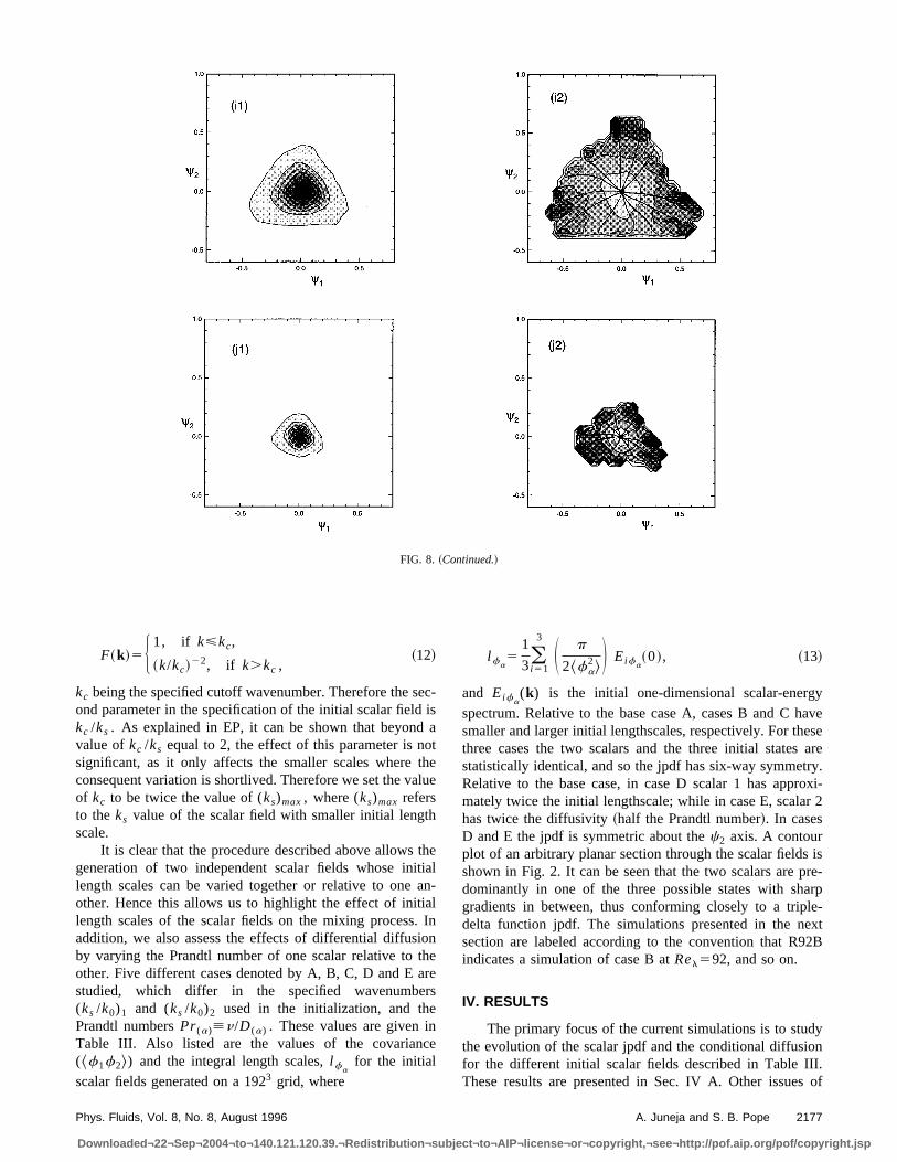
FIG. 8. Same as Fig. 4, but for R92E simulations.
2175Phys. Fluids, Vol. 8, No. 8, August 1996 A. Juneja and S. B. Pope
Downloaded¬22¬Sep¬2004¬to¬140.121.120.39.¬Redistribution¬subject¬to¬AIP¬license¬or¬copyright,¬see¬http://pof.aip.org/pof/copyright.jsp
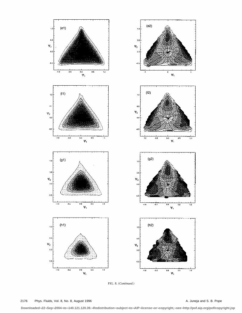
FIG. 8. ~Continued.!
2176 Phys. Fluids, Vol. 8, No. 8, August 1996 A. Juneja and S. B. Pope
Downloaded¬22¬Sep¬2004¬to¬140.121.120.39.¬Redistribution¬subject¬to¬AIP¬license¬or¬copyright,¬see¬http://pof.aip.org/pof/copyright.jsp
F~k!5H 1, if k<kc,
~k/kc!22, if k.kc ,
~12!
kc being the specified cutoff wavenumber. Therefore the sec-ond parameter in the specification of the initial scalar field iskc /ks . As explained in EP, it can be shown that beyond avalue ofkc /ks equal to 2, the effect of this parameter is notsignificant, as it only affects the smaller scales where theconsequent variation is shortlived. Therefore we set the valueof kc to be twice the value of (ks)max, where (ks)max refersto theks value of the scalar field with smaller initial lengthscale.
It is clear that the procedure described above allows thegeneration of two independent scalar fields whose initiallength scales can be varied together or relative to one an-other. Hence this allows us to highlight the effect of initiallength scales of the scalar fields on the mixing process. Inaddition, we also assess the effects of differential diffusionby varying the Prandtl number of one scalar relative to theother. Five different cases denoted by A, B, C, D and E arestudied, which differ in the specified wavenumbers(ks /k0)1 and (ks /k0)2 used in the initialization, and thePrandtl numbersPr (a)[n/D (a) . These values are given inTable III. Also listed are the values of the covariance(^f1f2&) and the integral length scales,lfa
for the initialscalar fields generated on a 1923 grid, where
lfa51
3(i51
3 S p
2^fa2& D Eifa
~0!, ~13!
and Eifa(k) is the initial one-dimensional scalar-energy
spectrum. Relative to the base case A, cases B and C havesmaller and larger initial lengthscales, respectively. For thesethree cases the two scalars and the three initial states arestatistically identical, and so the jpdf has six-way symmetry.Relative to the base case, in case D scalar 1 has approxi-mately twice the initial lengthscale; while in case E, scalar 2has twice the diffusivity~half the Prandtl number!. In casesD and E the jpdf is symmetric about thec2 axis. A contourplot of an arbitrary planar section through the scalar fields isshown in Fig. 2. It can be seen that the two scalars are pre-dominantly in one of the three possible states with sharpgradients in between, thus conforming closely to a triple-delta function jpdf. The simulations presented in the nextsection are labeled according to the convention that R92Bindicates a simulation of case B atRel592, and so on.
IV. RESULTS
The primary focus of the current simulations is to studythe evolution of the scalar jpdf and the conditional diffusionfor the different initial scalar fields described in Table III.These results are presented in Sec. IV A. Other issues of
FIG. 8. ~Continued.!
2177Phys. Fluids, Vol. 8, No. 8, August 1996 A. Juneja and S. B. Pope
Downloaded¬22¬Sep¬2004¬to¬140.121.120.39.¬Redistribution¬subject¬to¬AIP¬license¬or¬copyright,¬see¬http://pof.aip.org/pof/copyright.jsp
interest which are studied involve whether or not the scalarfields reach a self-similar state~Sec. IV B! and the rate ofdecay of the scalar variance and dissipation at large times~Sec. IV C!. We shall present detailed results from the R92Asimulations, where the initial length scales and the diffusivityfor the two scalar fields are the same. For the other cases, weshall highlight the differences~if any! in the scalar mixingprocess caused by a change in either the initial length scaleor the diffusivity. Except where noted, the results are fromsimulations utilizing the 1923 grid atRel592, i.e., R92.
It has been observed in some of the prior simulations~for example, EP! and experiments that for the mixing of asingle scalar with varying initial length scales~but the sameinitial pdf!, the evolution states of the scalar pdf are approxi-mately invariant if they are computed at fixed values off8/f08 . Here f8 represents the root mean square~r.m.s.!value of the scalar at the given time andf08 is the r.m.s.value at timet50 ~initial state!, the r.m.s. values being com-puted by taking the square root of the volume averaged sca-lar variance. Hence in the present simulations, we output the
various statistics at fixed values of the r.m.s.F[(f8/f08)1where the subscript 1 denotes that the ratio is computed forthe first scalar. Figure 3 shows a plot of the evolution of thescalar r.m.s (f8) and volume averaged scalar dissipation@^ef&[D^¹f(x,t).¹f(x,t)&# from the R92A simulations.Time is normalized by the large eddy-turnover time, i.e.t*5tu/ l . It can be seen that, in this case where the initiallength scales of the two scalars are identical, the evolution off8 and ^ef& are also quite similar—the differences beingentirely due to statistical variability.
A. Evolution of scalar jpdf and conditional diffusion
The scalar joint probability density function,P(c;t), iscomputed at specified timest by dividing thec1-c2 samplespace into 60360 intervals and then forming a histogramusing the values of the two scalars at each grid point. Asthere are about seven million grid points, the jpdf can beexpected to have relatively small statistical errors. The jpdfis easily represented as a contour plot in the two-dimensionalsample space.
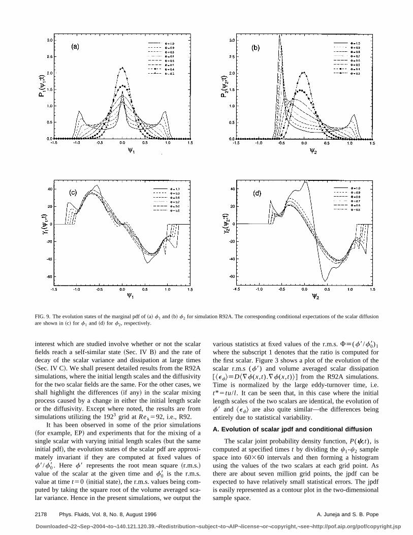
FIG. 9. The evolution states of the marginal pdf of~a! f1 and~b! f2 for simulation R92A. The corresponding conditional expectations of the scalar diffusionare shown in~c! for f1 and ~d! for f2, respectively.
2178 Phys. Fluids, Vol. 8, No. 8, August 1996 A. Juneja and S. B. Pope
Downloaded¬22¬Sep¬2004¬to¬140.121.120.39.¬Redistribution¬subject¬to¬AIP¬license¬or¬copyright,¬see¬http://pof.aip.org/pof/copyright.jsp
As mentioned earlier, for homogeneous scalar fields inhomogeneous turbulence, the primary quantity determiningthe evolution of the scalar jpdf is the expectation of the dif-fusion conditioned on the scalar value@see Eq.~2!#. Thisconditional expectation is estimated by generating a histo-gram of the scalar values weighted by the diffusion of eachof the two scalars at the same point. The value of each com-ponent of this vector function is then divided by the un-weighted histogram value of the scalar fields in the appropri-ate interval to yield the estimate ofg(c,t). The conditionaldiffusion ga(c,t)5^D (a)¹
2fauf(x,t)5c& is the expectedrate of change offa , conditioned onf5c, and henceg5(g1 ,g2) corresponds to a ‘‘velocity’’ in compositionspace. The results are shown as contour plots of the ‘‘speed’’ugu and of the ‘‘streamlines,’’ which are lines in thec1-c2
plane that are everywhere parallel tog. The jpdf evolves byprobability flowing along the ‘‘streamlines’’ at the ‘‘speed’’ugu.
Figure 4 shows the scalar jpdf and the conditional diffu-sion for the base case R92A simulations at r.m.s.F51.0,0.9,0.8,0.7,0.6,0.5,0.4,0.3,0.2 and 0.1, respectively.~Plate 1 shows the same plot in color atF51.0,0.8,0.6, and0.4 along with contour plots of a planar slice through theinitial scalar fields.! It may be seen from Figs. 4~a1!–4~d1!that at early times the jpdf evolves by probability flowingfrom the three delta functions along the lines joining them.This picture is confirmed by the streamline patterns on Figs.4~a2!–4~d2!. The streamlines accounting for the bulk ofprobability flow are nearly coincident with the sides of thetriangle. Note that except for Fig. 4~a2! which is an artifactof the initial condition, the contour plot of the ‘‘speed’’uguhas maxima along the three edges of the triangle; and that,by symmetry, there is a straight streamline from each deltafunction to the origin for all time. In physical space, it is themixing across the initial interfaces betweenpairs of blobs
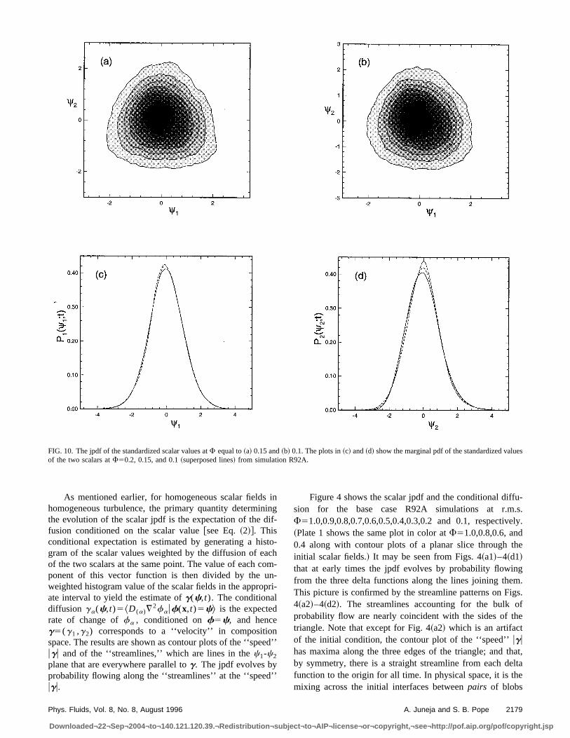
FIG. 10. The jpdf of the standardized scalar values atF equal to~a! 0.15 and~b! 0.1. The plots in~c! and~d! show the marginal pdf of the standardized valuesof the two scalars atF50.2, 0.15, and 0.1~superposed lines! from simulation R92A.
2179Phys. Fluids, Vol. 8, No. 8, August 1996 A. Juneja and S. B. Pope
Downloaded¬22¬Sep¬2004¬to¬140.121.120.39.¬Redistribution¬subject¬to¬AIP¬license¬or¬copyright,¬see¬http://pof.aip.org/pof/copyright.jsp
that accounts for the triangular shape of the pdf at earlytimes. It is worth noting that for a single-scalar case, a dif-fusive layer betweenf1521.0 andf151.0 with an errorfunction profile has a maxima ofu¹2f1u atc1560.68. Thiscan be qualitatively observed in the contour plots in Figs.4~b2!–4~d2! in the present case. As time evolves~e.g.F50.7! the interior of the triangular jpdf fills in, and atF50.6 the jpdf is remarkably uniform. Eswaran and Pope1
also observed an approximately uniform pdf in the single-scalar case. Subsequently the peak of the jpdf is at the origin,and the triangular shape gradually changes to a circle at largetimes.
It is interesting to observe that if the jpdf decays as ajoint normal distribution~as it approximately does for largetimes,F<0.1 say, see Sec. IV B!, then the streamlines areradii, and the speed is linearly proportional to the distancefrom the origin. The simplest possible mixing model~IEM22
or LMSE23! predicts this behavior at all times. Clearly, forthe times shown in Fig. 4, both in direction and magnitude,the conditional diffusion is very different from this predic-tion. To provide a better guide for modeling efforts and toprovide quantitative information on the evolution of condi-
tional diffusion, we plot the normalized value of its indi-vidual components in Fig. 5 along four lines in thec1-c2
plane as a function of time; the normalization ofg1 andg2 isperformed by dividing its value byef /2f8 for the first sca-lar at the given time.
Figure 6 shows the same plot as Fig. 4 from the R92Bsimulations. The evolution of the scalar jpdf and conditionaldiffusion look quite similar to Fig. 4 even though the initiallength scales of the scalar fields B are different from those inA. We also carried out simulations employing the initial sca-lar field C (ks /k052 and Pr50.7 for both scalars!. Theplots ~not shown here! are again very much like Figs. 4 and6 and it can be concluded that, if the scalar initializationscheme described in Sec. III is employed, then as long as theinitial length scales of the two scalars fields are the samerelative to one another, it does not matter whether the valueof the length scale itself is varied between simulations, if oneis interested in the evolution states of the scalar jpdf andconditional diffusion at fixed values ofF.
In order to assess the effect of varying the initial lengthscales of the scalar fields relative to one another, we next
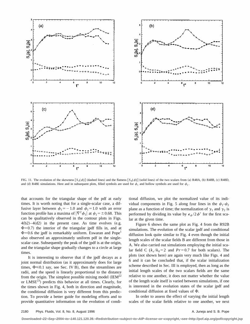
FIG. 11. The evolution of the skewness@S3(f)# ~dashed lines! and the flatness@S4(f)# ~solid lines! of the two scalars from~a! R48A, ~b! R48B, ~c! R48D,and ~d! R48E simulations. Here and in subsequent plots, filled symbols are used forf1 and hollow symbols are used forf2 .
2180 Phys. Fluids, Vol. 8, No. 8, August 1996 A. Juneja and S. B. Pope
Downloaded¬22¬Sep¬2004¬to¬140.121.120.39.¬Redistribution¬subject¬to¬AIP¬license¬or¬copyright,¬see¬http://pof.aip.org/pof/copyright.jsp
present the results from R92D simulations employing theinitial scalar field D in which (ks /k0)152 and (ks /k0)254while Pr50.7 for both scalars. Figure 7 shows the evolutionof the scalar jpdf and the conditional diffusion for this case.It is seen that the mixing is faster in thec2 direction. This isto be expected as the scalar with a smaller initial length scaletends to mix more rapidly. In this case, the jpdf spreadsmuch more slowly along the edge of the triangle alignedwith the c1 axis when compared to the other two edges ofthe triangle. Again the trend is explained by looking at thethe plots for the conditional diffusion. Most of the stream-lines indicate a faster initial mixing along thec2 axis whichdictates the evolution of the scalar jpdf.
If, on the other hand, the diffusivity of the second scalaris set to twice the value of that for the first scalar whilekeeping the initial length scales to be the same~scalar fieldE!, a similar albeit much less pronounced effect on the evo-lution of the jpdf can be observed~Fig. 816!. The secondscalar again tends to mix a little faster than the first scalarand this causes the edge of the triangle parallel to thec1 axisto bend more towards the origin near the center than theother two edges. The resulting concave shape of the edge ofparallel to thec1 axis and the convex nature of the other twoedges is best seen in Figs. 8~c1! and 8~d1!. It is worth notingthat the increase in diffusivity causes the scalar jpdf at early
times to stretch outside the triangle described by the initialstate jpdf, unlike the previous cases. Once again, the jpdf hasa somewhat flat distribution atF50.6, before it begins tolose its triangular shape. The corresponding plots for theconditional diffusion show much more clearly the effect ofchanged diffusivity, when compared to those for scalars withequal diffusivity and equal length scales. It is also useful tonote that changing the length scale and the diffusivity of thescalars are two completely different issues even though theireffects in the present case are somewhat similar. The effectdue to the change in length scale is expected to be presenteven as the Reynolds number goes to infinity, whereas theeffect due to increased diffusivity should gradually disappearas the Reynolds number is increased.
We also independently computed the marginal pdf’s ofthe two scalars, P1(c1 ,t) and P2(c2 ,t) and theconditional expectation of diffusion for the individualscalars @g1(c1 ,t)5^¹2f1uf15c1& and g2(c2 ,t)5^¹2f2uf25c2&] by forming histograms using 100 sam-pling intervals. Figure 9 shows the respective plots from theR92A simulations. It can be observed from Figs. 9~a! and9~b! that, even though the initial shape for the marginal pdf’sfor the two scalar are quite different from one another, theyassume a similar near-Gaussian shape by the timeF50.3.Also, the plots of the individual conditional scalar diffusion
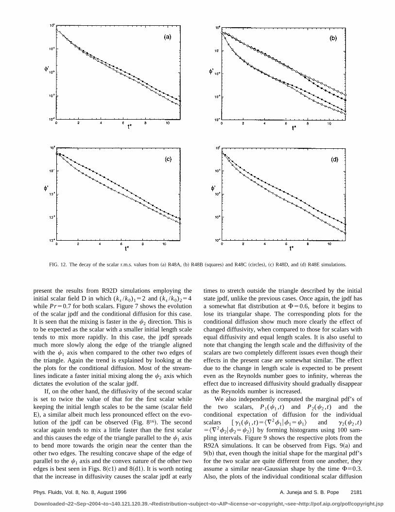
FIG. 12. The decay of the scalar r.m.s. values from~a! R48A, ~b! R48B ~squares! and R48C~circles!, ~c! R48D, and~d! R48E simulations.
2181Phys. Fluids, Vol. 8, No. 8, August 1996 A. Juneja and S. B. Pope
Downloaded¬22¬Sep¬2004¬to¬140.121.120.39.¬Redistribution¬subject¬to¬AIP¬license¬or¬copyright,¬see¬http://pof.aip.org/pof/copyright.jsp
indicate a linear region in the center at larger times~i.e.,smaller values ofF!, as has been observed before both nu-merically and experimentally. As a final remark, we exam-ined the evolution of the scalar jpdf and conditional diffusionon the smaller 963 grid at a Taylor scale Reynolds number ofRel548. The results look very similar and this suggests thatthe mixing process is not strongly influenced~at least quali-tatively! by the Reynolds number in the range considered.
B. Self-similarity at later times
Next, we address the issue of the self-similarity of thescalar fields at larger times. This is done by examining thestandardized joint and the marginal pdf’s of the two scalars -i.e., the pdf’s of the two scalars normalized by their respec-tive r.m.s. values at the given time. The plots of the standard-ized jpdf’s atF50.15 and 0.1 are shown in Figs. 10~a! and10~b!. These results have been extracted from the R92Asimulations. The shapes of the two jpdf’s are quite similar,and in general it was found that the standardized jpdf’s havea statistically self-similar shape which is close to a joint-normal for F<0.25. It should however be noted that forcases D and E, this jpdf has different variances for the twoscalars at all times, i.e.f18 is greater thanf28 ~see Fig. 12!.The plot of the standardized marginal pdf’s of the two scalars
~once again normalized by the respective r.m.s. values! atthree different values ofF equal to 0.20, 0.15, and 0.1 areshown superimposed on each other in Figs. 10~c! and 10~d!.The different curves seem to lie on top of each other indicat-ing that a self-similar state has been reached.
Another way of examining the self-similar state of a pdfis to plot the value of the normalized moments of the pdf asa function of the time. Since this self-similarity will be evi-dent only at larger times, we ran simulations for about twelvelarge-eddy turnover times, but on a smaller 963 grid in orderto keep computational costs low. Figure 11 shows the evo-lution of the normalized third and fourth moments~skewnessand flatness respectively! of the marginal scalar pdfs.~HereSm@q# denotes themth normalized central moment of therandom variableq.) It is seen that at the initial time, the firstscalar has zero skewness and the second scalar has a positiveskewness of around 0.75 while the flatness for both is closeto 1.8 in all cases. As the simulation progresses, the secondscalar loses its positive skewness, and after a while the skew-ness of both scalars is found to oscillate around zero,whereas the flatness initially rises and then fluctuates arounda value close to 3.5 independently of the choice of the initialscalar fields employed in the simulations.~The statistical
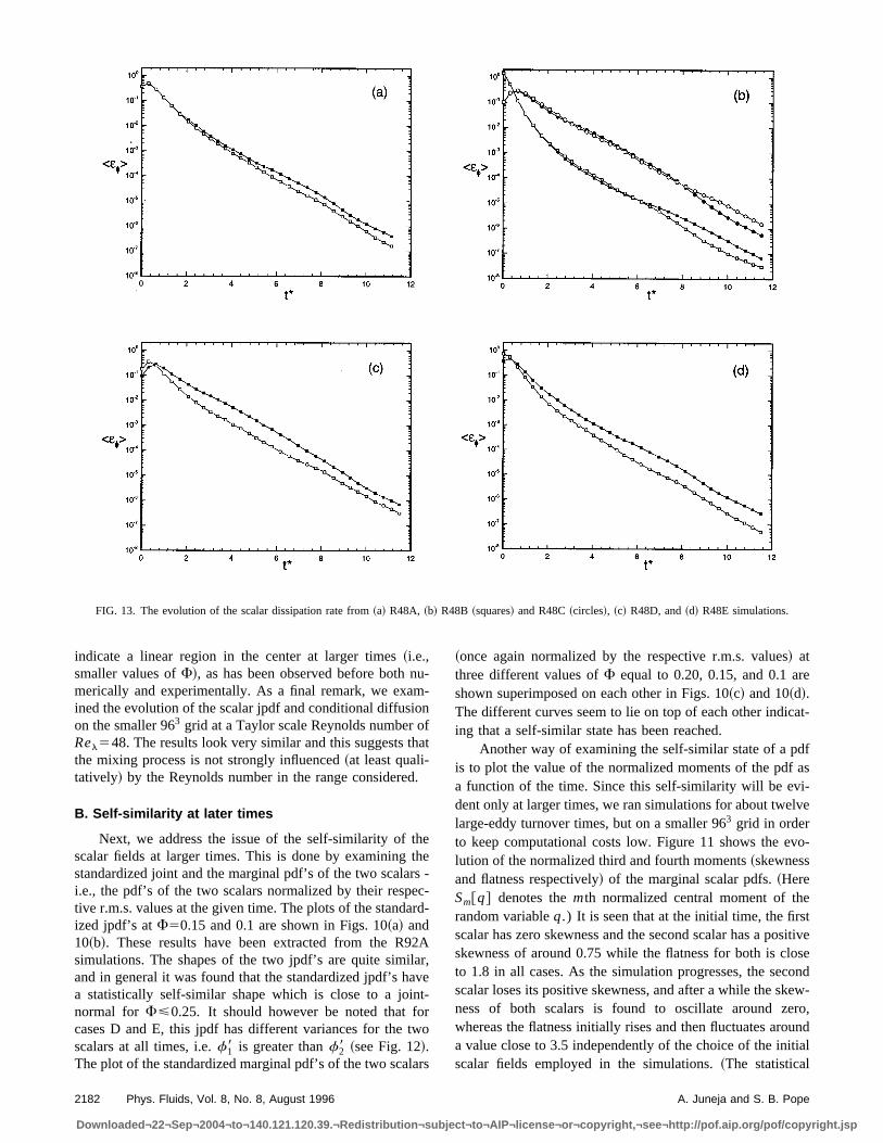
FIG. 13. The evolution of the scalar dissipation rate from~a! R48A, ~b! R48B ~squares! and R48C~circles!, ~c! R48D, and~d! R48E simulations.
2182 Phys. Fluids, Vol. 8, No. 8, August 1996 A. Juneja and S. B. Pope
Downloaded¬22¬Sep¬2004¬to¬140.121.120.39.¬Redistribution¬subject¬to¬AIP¬license¬or¬copyright,¬see¬http://pof.aip.org/pof/copyright.jsp
variability precludes precise statements concerning any de-parture from Gaussianity.!
C. Evolution of scalar variance and dissipation
In the case of a single scalar with a specified initial pdf,the initial decay rate of the scalar variance and dissipation isknown to depend on the initial length scale of the scalar.24
However, at large times, these decay rates may become simi-lar ~in stationary turbulence!1,25 leading to a universal valueof the mechanical-to-scalar time-scale ratio defined byr[(^ef&/^f2&)/@e/(3u2)#. Hence it is of interest to inves-tigate the decay rates for the present problem where the mar-ginal pdf’s of the two scalars are also significantly differentfrom one another. Again, the results are extracted from thesimulations performed on the smaller 963 grid atRel548 tofacilitate longer runs. The decay of the r.m.s. values of thetwo scalars for different initial scalar fields is plotted in Fig.12. It is seen that for initial scalar fields A, B, C@Figs. 12~a!and 12~b!#, where the length scales of the two scalars areequal relative to one another, the initial rate of decay off18and f28 is almost indistinguishable. At large times, thereseems to be some difference in the decay rate but we canattribute that to statistical variability~see Fig. 8 in EP!. In
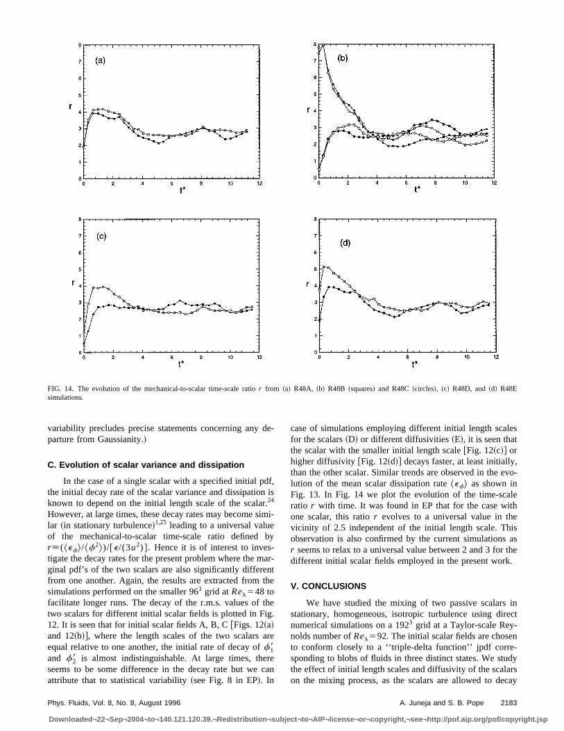
case of simulations employing different initial length scalesfor the scalars~D! or different diffusivities~E!, it is seen thatthe scalar with the smaller initial length scale@Fig. 12~c!# orhigher diffusivity @Fig. 12~d!# decays faster, at least initially,than the other scalar. Similar trends are observed in the evo-lution of the mean scalar dissipation rate^ef& as shown inFig. 13. In Fig. 14 we plot the evolution of the time-scaleratio r with time. It was found in EP that for the case withone scalar, this ratior evolves to a universal value in thevicinity of 2.5 independent of the initial length scale. Thisobservation is also confirmed by the current simulations asr seems to relax to a universal value between 2 and 3 for thedifferent initial scalar fields employed in the present work.
V. CONCLUSIONS
We have studied the mixing of two passive scalars instationary, homogeneous, isotropic turbulence using directnumerical simulations on a 1923 grid at a Taylor-scale Rey-nolds number ofRel592. The initial scalar fields are chosento conform closely to a ‘‘triple-delta function’’ jpdf corre-sponding to blobs of fluids in three distinct states. We studythe effect of initial length scales and diffusivity of the scalarson the mixing process, as the scalars are allowed to decay
FIG. 14. The evolution of the mechanical-to-scalar time-scale ratior from ~a! R48A, ~b! R48B ~squares! and R48C~circles!, ~c! R48D, and~d! R48Esimulations.
2183Phys. Fluids, Vol. 8, No. 8, August 1996 A. Juneja and S. B. Pope
Downloaded¬22¬Sep¬2004¬to¬140.121.120.39.¬Redistribution¬subject¬to¬AIP¬license¬or¬copyright,¬see¬http://pof.aip.org/pof/copyright.jsp
from their prescribed initial state. In all the cases considered,the scalar jpdf initially tends to spread mainly along theedges of the triangle formed by the three delta functions. Inphysical space this corresponds to the mixing between adja-cent pairs of blobs. Further, the decay of the scalar fieldscauses the triangle to shrink slowly towards the origin. Whenplotted at fixed values of the r.m.s.F, the evolution states ofthe jpdf do not depend on the initial length scale of thescalars, as long as they are the same for both. The effect ofchanging the length scale or diffusivity of one scalar relativeto the other manifests itself in the form of faster mixing inthe direction of the scalar with the smaller length scale or thehigher diffusivity, respectively. Another notable feature isthat the scalar jpdf assumes a relatively flat triangular distri-bution, before it loses the inherited triangular shape from theinitial state and starts evolving to a near joint-normal form.These trends in the evolution of the jpdf are explained byexamining the corresponding plots for the conditional scalardiffusion, which can be used to formulate better mixingmodels for the multi-scalar case.
ACKNOWLEDGMENTS
The work was supported in part by the Department ofEnergy under Grant DE-FG02-90ER 14128 and by the Cor-nell Center for Theory and Simulation in Science and Engi-neering.
1V. Eswaran and S. B. Pope, ‘‘Direct numerical simulations of the turbulentmixing of a passive scalar,’’ Phys. Fluids31, 506 ~1988!.
2K. R. Sreenivasan, S. Tavoularis, R. Henry, and S. Corrsin, ‘‘Temperaturefluctuations and scales in grid-generated turbulence,’’ J. Fluid Mech.100,597 ~1980!.
3Jayesh and Z. Warhaft, ‘‘Probability distributions, conditional dissipation,and transport of passive temperature fluctuations in grid-generated turbu-lence,’’ Phys. Fluids A4, 2292~1992!.
4P. E. Dimotakis, R. C. M. Lye, and D. A. Papantoniou, ‘‘Structure anddynamics of round turbulent jets,’’ Phys. Fluids28, 3185~1983!.
5R. R. Prasad and K. R. Sreenivasan, ‘‘Quantitative three-dimensional im-aging and the structure of passive scalar fields in fully turbulent flows,’’ J.Fluid Mech.216, 1 ~1990!.
6W. J. A. Dahm, K. B. Sutherland, and K. A. Buch, ‘‘Direct high-resolution4-dimensional measurements of the fine scale structure of Sc greater-than
1 molecular mixing in turbulent flows,’’ Phys. Fluids A3, 1115~1991!.7R. M. Kerr, ‘‘Higher-order derivative correlations and alignment of small-scale structures in isotropic numerical turbulence,’’ J. Fluid Mech.153, 31~1985!.
8G. A. Blaisdell, N. N. Mansour, and W. C. Reynolds, ‘‘Compressibilityeffects on the passive scalar flux within homogeneous turbulence,’’ Phys.Fluids6, 3498~1994!.
9A. Pumir, ‘‘A numerical study of the mixing of a passive scalar in threedimensions in the presence of a mean gradient,’’ Phys. Fluids6, 2118~1994!.
10J. R. Chasnov, ‘‘Similarity states of passive scalar transport in buoyancy-generated turbulence,’’ Phys. Fluids7, 1498~1995!; ‘‘Similarity states ofpassive scalar transport in isotropic turbulence,’’6, 1036~1994!.
11S. B. Pope, ‘‘PDF methods for turbulent reactive flows,’’ Prog. EnergyCombust. Sci.11, 119 ~1985!.
12S. B. Pope, ‘‘Mapping closures for turbulent mixing and reaction,’’ Theo.Comput. Fluid Dyn.2, 255 ~1991!.
13A. R. Kerstein, ‘‘Linear-Eddy modeling of turbulent transport: Part II.Application to shear layer mixing,’’ Combust. Flame75, 397 ~1989!.
14A. Sirivat and Z. Warhaft, ‘‘The mixing of passive helium and tempera-ture fluctuations in grid turbulence,’’ J. Fluid Mech.120, 475 ~1982!.
15Z. Warhaft, ‘‘The use of dual heat injection to infer scalar covariancedecay in grid turbulence’’ J. Fluid Mech.104, 93 ~1981!.
16P. K. Yeung and S. B. Pope, ‘‘Differential diffusion of passive scalars inisotropic turbulence,’’ Phys. Fluids A5, 2467~1993!.
17J. R. Saylor, ‘‘Differential diffusion in turbulent and oscillatory non-turbulent water flows,’’ PhD thesis, Yale University, 1993.
18R. S. Rogallo, ‘‘Numerical experiments in homogeneous turbulence,’’NASA TM-81315, 1981.
19V. Eswaran and S. B. Pope, ‘‘An examination of forcing in direct numeri-cal simulations of turbulence,’’ Comput. Fluids16, 257 ~1988!.
20P. K. Yeung and S. B. Pope, ‘‘Lagrangian Statistics from direct numericalsimulations of isotropic turbulence,’’ J. Fluid Mech.207, 531 ~1989!.
21P. K. Yeung and C. A. Moseley, ‘‘A message-passing, distributed memoryparallel algorithm for direct numerical simulation of turbulence with par-ticle tracking,’’ in Parallel Computational Fluid Dynamics: Implementa-tion and Results Using Parallel Computers, edited by A. Ecer, J. Periaux,N. Satofuka and S. Taylor~Elsevier Science, New York, 1995!.
22J. Villermaux and J. C. Devillon, inProceedings of the 2nd InternationalSymposium on Chemical Reaction Engineering~Elsevier Science, NewYork, 1972!.
23C. Dopazo and E. E. O’Brien, ‘‘An approach to the autoignition of aturbulent mixture,’’ Acta Astronaut.1, 1239~1974!.
24Z. Warhaft and J. L. Lumley, ‘‘An experimental study of the decay oftemperature fluctuations in grid generated turbulence,’’ J. Fluid Mech.88,659 ~1978!.
25P. A. Durbin, ‘‘Analysis of the decay of temperature fluctuations in iso-tropic turbulence,’’ Phys. Fluids25, 1328~1982!.
2184 Phys. Fluids, Vol. 8, No. 8, August 1996 A. Juneja and S. B. Pope
Downloaded¬22¬Sep¬2004¬to¬140.121.120.39.¬Redistribution¬subject¬to¬AIP¬license¬or¬copyright,¬see¬http://pof.aip.org/pof/copyright.jsp