A dual view of Markov processes - McGill University School ...prakash/Talks/irif-2.pdf · A dual view of Markov processes Prakash Panangaden1 1School of Computer Science McGill University

A dual view of Markov processes

Prakash Panangaden1

1School of Computer ScienceMcGill University

IRIF Lecture Series Jan 2018

Panangaden (McGill University) Lecture 2 IRIF 18th January 2018 1 / 53

Overview

1 Present a “new” view of Markov processes as functiontransformers

2 Show a beautiful functorial presentation of expectation values3 Make bisimulation and approximation live in the same universe4 Minimal realization theory5 Approximation


Collaborators

Philippe Chaput, Vincent Danos and Gordon Plotkin.


What are labelled Markov processes?

Labelled Markov processes are probabilistic versions of labelledtransition systems. Labelled transition systems where the finalstate is governed by a probability distribution - no otherindeterminacy.All probabilistic data is internal - no probabilities associated withenvironment behaviour.We observe the interactions - not the internal states.In general, the state space of a labelled Markov process maybe a continuum.


Motivation

Model and reason about systems with continuous state spaces.

hybrid control systems; e.g. flight management systems.telecommunication systems with spatial variation; e.g. cellphones.performance modelling.probabilistic process algebra with recursion.


Formal Definition of LMPs

An LMP is a tuple (S,Σ,L,∀α ∈ L.τα) where τα : S×Σ −→ [0, 1] is atransition probability function such that∀s : S.λA : Σ.τα(s,A) is a subprobability measureand∀A : Σ.λs : S.τα(s,A) is a measurable function.


Logical Characterization

L0 ::== T|φ1 ∧ φ2|〈a〉qφ

We say s |= 〈a〉qφ iff

∃A ∈ Σ.(∀s′ ∈ A.s′ |= φ) ∧ (τa(s,A) > q).

Two systems are bisimilar iff they obey the same formulas of L.[DEP 1998 LICS, I and C 2002]


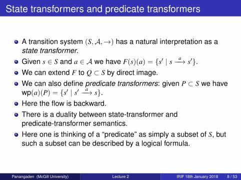
State transformers and predicate transformers

A transition system (S,A,→) has a natural interpretation as astate transformer.Given s ∈ S and a ∈ A we have F(s)(a) = {s′ | s a−−→ s′}.We can extend F to Q ⊂ S by direct image.We can also define predicate transformers: given P ⊂ S we havewp(a)(P) = {s′ | s′ a−−→ s}.Here the flow is backward.There is a duality between state-transformer andpredicate-transformer semantics.Here one is thinking of a “predicate” as simply a subset of S, butsuch a subset can be described by a logical formula.


Logic and Probability

Classical logic GeneralizationTruth values {0, 1} Probabilities [0, 1]

Predicate Random variableState Distribution

The satisfaction relation |= Integration∫


The “predicate transformer” view of Markov processes

Recall, a Markov kernel τ from (X,Σ) to (Y,Λ) is a mapτ : X × Λ −→ [0, 1] which is measurable in its first argument and a(subprobability) measure in the second argument.Let f be a real-valued function on Y. We defineBτ (f )(x) =

∫Y f (y)τ(x, dy); this is playing the role analogous to a

predicate transformer. It is in fact an expectation transformer.Bτ (f )(x) is the expectation value of f after a step given that thesystem was at x before the step.


The general plan

We are going to view Markov processes as function transformersrather than as state transformers.We will take the backward view; we could, perhaps equally well,have developed a forward view but we have not done so.Measure theory works much better when one deals withmeasurable functions rather than “points” and measures.We never have to worry about “almost everywhere” and othersuch nonsense.Because of our backward view, bisimulation becomes a cospaninstead of a span. But this actually makes everything easier!We can develop a theory of bisimulation, logical characterization,approximation and minimal realization in this framework.


Banach spaces

A norm on a vector space V is a function ‖·‖ : V −→ R≥0 such that:1 ‖v‖ = 0 iff v = 02 ‖r · v‖ =| r | ‖v‖ and3 ‖x + y‖ ≤ ‖x‖+ ‖y‖.

The norm induces a metric: d(u, v) = ‖u− v‖ and, hence, atopology. This topology is called the norm topology.If V is complete in this metric it is called a Banach space.In quantum mechanics the state spaces are Hilbert spaces –hence automatically Banach spaces – but the spaces of operatorsare not Hilbert spaces, they are Banach spaces.


Maps between Banach spaces

A linear map T : U −→ V is bounded if there exists a positive realnumber α such that ∀u ∈ U, ‖Tu‖ ≤ α ‖u‖.A lineap map between normed spaces is continuous iff it isbounded.Given a bounded linear map between normed spaces T : U −→ Vwe define ‖T‖ = sup {‖Tu‖ | u ∈ U, ‖u‖ ≤ 1}.This is a norm on the space of bounded linear maps and is calledthe operator norm.With this norm the space of bounded linear maps betweenBanach spaces forms a Banach space.


Duality for Banach spaces

The space of bounded (= continuous) linear maps from V, aBanach space, to R is itself a Banach space, called the dualspace, V∗.For any two vector spaces U,V we say that they are in algebraicduality if there is a bilinear form 〈·, ·〉 : U × V −→ R such thatspaces of functionals 〈·, V〉 and 〈U, ·〉 separates points of U andV.We say two Banach spaces are in duality if 〈·, V〉 ⊆ U∗ and〈U, ·〉 ⊆ V∗.For V a Banach space, the spaces V and V∗ are in duality.The bilinear form is 〈v, φ〉 = φ(v).There is a canonical injection ι : V −→ V∗∗; if this is an isometry wesay that the Banach space V is reflexive.Infinite dimensional Banach spaces are not necessarily reflexive.Finite dimensional Banach spaces are always reflexive.


What are cones?

Want to combine linear structure with order structure.If we have a vector space with an order ≤ we have a naturalnotion of positive and negative vectors: x ≥ 0 is positive.What properties do the positive vectors have? Say P ⊂ V are thepositive vectors, we include 0.Then for any positive v ∈ P and positive real r, rv ∈ P. For u, v ∈ Pwe have u + v ∈ P and if v ∈ P and −v ∈ P then v = 0.We define a cone C in a vector space V to be a set with exactlythese conditions.Any cone defines a order by u ≤ v if v− u ∈ C.Unfortunately for us, many of the structures that we want to look atare cones but are not part of any obvious vector space: e.g. themeasures on a space.We could artificially embed them in a vector space, for example,by introducing signed measures.


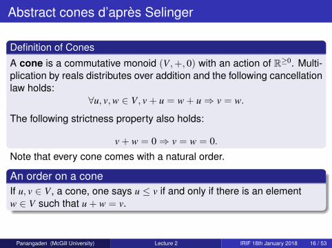
Abstract cones d’après Selinger

Definition of Cones

A cone is a commutative monoid (V,+, 0) with an action of R≥0. Multi-plication by reals distributes over addition and the following cancellationlaw holds:

∀u, v,w ∈ V, v + u = w + u⇒ v = w.

The following strictness property also holds:

v + w = 0⇒ v = w = 0.

Note that every cone comes with a natural order.

An order on a coneIf u, v ∈ V, a cone, one says u ≤ v if and only if there is an elementw ∈ V such that u + w = v.


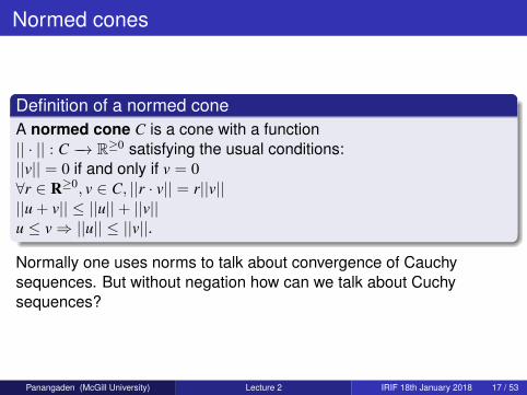
Normed cones

Definition of a normed coneA normed cone C is a cone with a function|| · || : C −→ R≥0 satisfying the usual conditions:||v|| = 0 if and only if v = 0∀r ∈ R≥0, v ∈ C, ||r · v|| = r||v||||u + v|| ≤ ||u||+ ||v||u ≤ v⇒ ||u|| ≤ ||v||.

Normally one uses norms to talk about convergence of Cauchysequences. But without negation how can we talk about Cuchysequences?


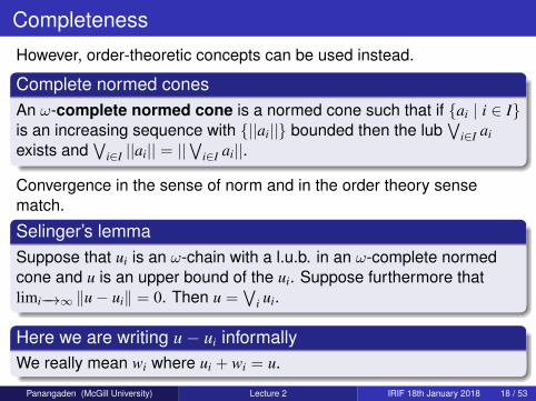
Completeness

However, order-theoretic concepts can be used instead.

Complete normed conesAn ω-complete normed cone is a normed cone such that if {ai | i ∈ I}is an increasing sequence with {||ai||} bounded then the lub

∨i∈I ai

exists and∨

i∈I ||ai|| = ||∨

i∈I ai||.

Convergence in the sense of norm and in the order theory sensematch.

Selinger’s lemmaSuppose that ui is an ω-chain with a l.u.b. in an ω-complete normedcone and u is an upper bound of the ui. Suppose furthermore thatlimi−→∞ ‖u− ui‖ = 0. Then u =

∨i ui.

Here we are writing u− ui informallyWe really mean wi where ui + wi = u.


Maps between cones

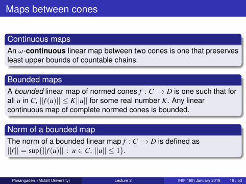
Continuous mapsAn ω-continuous linear map between two cones is one that preservesleast upper bounds of countable chains.

Bounded mapsA bounded linear map of normed cones f : C −→ D is one such that forall u in C, ||f (u)|| ≤ K||u|| for some real number K. Any linearcontinuous map of complete normed cones is bounded.

Norm of a bounded mapThe norm of a bounded linear map f : C −→ D is defined as||f || = sup{||f (u)|| : u ∈ C, ||u|| ≤ 1}.


A category of normed cones

The ambient categoryThe ω-complete normed cones, along with ω-continuous linear maps,form a category which we shall denote ωCC.

The subcategory of interestwe define the subcategory ωCC1: the norms of the maps are allbounded by 1. Isomorphisms in this category are always isometries.


Dual cones

Dual coneGiven an ω-complete normed cone C, its dual C∗ is the set of allω-continuous linear maps from C to R+. We define the norm on C∗ tobe the operator norm.

Basic factsC∗ is an ω-complete normed cone as well, and the cone ordercorresponds to the point wise order.


The duality functor

In ωCC, the dual operation becomes a contravariant functor.If f : C −→ D is a map of cones, we define f ∗ : D∗ −→ C∗ as follows:given a map L in D∗, we define a map f ∗L in C∗ as f ∗L(u) = L(f (u)).


How does this compare with Banach spaces?

This dual is stronger than the dual in usual Banach spaces, where weonly require the maps to be bounded. For instance, it turns out that thedual to L+

∞(X) (to be defined later) is isomorphic to L+1 (X), which is not

the case with the Banach space L∞(X).


Cones that we use I

If µ is a measure on X, then one has the well-known Banachspaces L1 and L∞.These can be restricted to cones by considering the µ-almosteverywhere positive functions.We will denote these cones by L+

1 (X,Σ, µ) and L+∞(X,Σ).

These are complete normed cones.


Cones that we use II

Let (X,Σ, p) be a measure space with finite measure p. We denotebyM�p(X), the cone of all measures on (X,Σ, p) that areabsolutely continuous with respect to p

If q is such a measure, we define its norm to be q(X).M�p(X) is also an ω-complete normed cone.The conesM�p(X) and L+

1 (X,Σ, p) are isometrically isomorphicin ωCC.We writeMp

UB(X) for the cone of all measures on (X,Σ) that areuniformly less than a multiple of the measure p: q ∈Mp

UB meansthat for some real constant K > 0 we have q ≤ Kp.The conesMp

UB(X) and L+∞(X,Σ, p) are isomorphic.


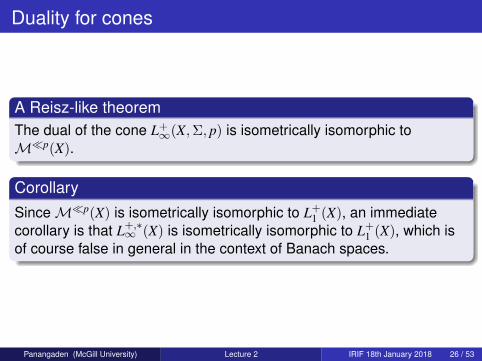
Duality for cones

A Reisz-like theoremThe dual of the cone L+

∞(X,Σ, p) is isometrically isomorphic toM�p(X).

CorollarySinceM�p(X) is isometrically isomorphic to L+

1 (X), an immediatecorollary is that L+,∗

∞ (X) is isometrically isomorphic to L+1 (X), which is

of course false in general in the context of Banach spaces.


Duality for cones II

Another Reisz-like theoremThe dual of the cone L+

1 (X,Σ, p) is isometrically isomorphic toMpUB(X).

CorollaryMp

UB(X) is isometrically isomorphic to L+∞(X), hence immediate

corollary is that L+,∗1 (X) is isometrically isomorphic to L+

∞(X).


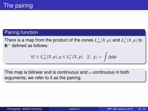
The pairing

Pairing function

There is a map from the product of the cones L+∞(X, p) and L+

1 (X, p) toR+ defined as follows:

∀f ∈ L+∞(X, p), g ∈ L+

1 (X, p) 〈f , g〉 =

∫fgdp.

This map is bilinear and is continuous and ω-continuous in botharguments; we refer to it as the pairing.


Duality expressed via pairing

This pairing allows one to express the dualities in a very convenientway. For example, the isomorphism between L+

∞(X, p) and L+1 (X, p)

sends f ∈ L+∞(X, p) to λg.〈f , g〉 = λg.

∫fgdp.


Summary of cones

We fix a probability triple (X,Σ, p) and focus on six spaces of conesthat are based on them. They break into two natural groups of threeisomorphic spaces. The first three spaces are:A1 M�p(X) - the cone of all measures on (X,Σ, p) that are absolutely

continuous with respect to p,A2 L+

1 (X, p) - the cone of integrable almost-everywhere positivefunctions,

A3 L+,∗∞ (X, p) - the dual cone of the the cone of almost-everywhere

positive bounded measurable functions.


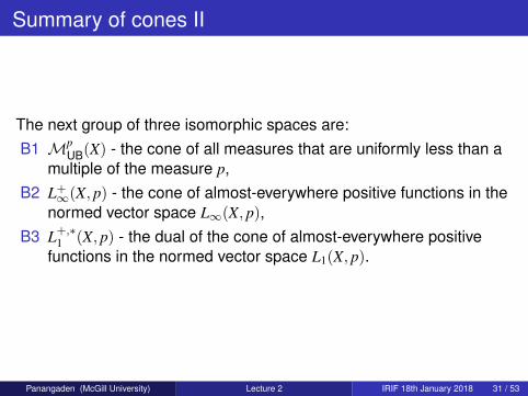
Summary of cones II

The next group of three isomorphic spaces are:B1 Mp

UB(X) - the cone of all measures that are uniformly less than amultiple of the measure p,

B2 L+∞(X, p) - the cone of almost-everywhere positive functions in the

normed vector space L∞(X, p),B3 L+,∗

1 (X, p) - the dual of the cone of almost-everywhere positivefunctions in the normed vector space L1(X, p).


Duality is the Key

M�p(X)

��

∼ // L+1 (X, p)oo

��

∼ // L+,∗∞ (X, p)oo

��Mp

UB

OO

∼ // L+∞(X, p)oo ∼ //

OO

L+,∗1 (X, p)

OO

oo

(1)

where the vertical arrows represent dualities and the horizontal arrowsrepresent isomorphisms.

Pairing function

There is a map from the product of the cones L+∞(X, p) and L+

1 (X, p) toR+ defined as follows:

∀f ∈ L+∞(X, p), g ∈ L+

1 (X, p) 〈f , g〉 =

∫fgdp.


Some notation

1 Given (X,Σ, p) and (Y,Λ) and a measurable function f : X −→ Y weobtain a measure q on Y by q(B) = p(f−1(B)). This is written Mf (p)and is called the image measure of p under f .

2 We say that a measure ν is absolutely continuous with respectto another measure µ if for any measurable set A, µ(A) = 0 impliesthat ν(A) = 0. We write ν � µ.


The Radon-Nikodym Theorem

The Radon-Nikodym theorem is a central result in measure theoryallowing one to define a “derivative” of a measure with respect toanother measure.

Radon-NikodymIf ν � µ, where ν, µ are finite measures on a measurable space (X,Σ)there is a positive measurable function h on X such that for everymeasurable set B

ν(B) =

∫B

h dµ.

The function h is defined uniquely up to a set of µ-measure 0. Thefunction h is called the Radon-Nikodym derivative of ν with respect toµ; we denote it by dν

dµ . Since ν is finite, dνdµ ∈ L+

1 (X, µ).


Notation for Radon-Nikodym

1 Given an (almost-everywhere) positive function f ∈ L1(X, p), we letf · p be the measure which has density f with respect to p.

2 Two identities that we get from the Radon-Nikodym theorem are:given q� p, we have dq

dp · p = q.given f ∈ L+

1 (X, p), df ·pdp = f

3 These two identities just say that the operations (−) · p and d(−)dp

are inverses of each other as maps between L+1 (X, p) and

M�p(X) the space of finite measures on X that are absolutelycontinuous with respect to p.


Expectation and conditional expectation

1 The expectation Ep(f ) of a measurable function f is the averagecomputed by

∫f dp and therefore it is just a number.

2 The conditional expectation is not a mere number but a randomvariable.

3 It is meant to measure the expected value in the presence ofadditional information.

4 The additional information takes the form of a sub-σ algebra, sayΛ, of Σ. The experimenter knows, for every B ∈ Λ, whether theoutcome is in B or not.

5 Now she can recompute the expectation values given thisinformation.


Formalizing conditional expectation

It is an immediate consequence of the Radon-Nikodym theoremthat such conditional expectations exist.

KolmogorovLet (X,Σ, p) be a measure space with p a finite measure, f be inL1(X,Σ, p) and Λ be a sub-σ-algebra of Σ, then there exists ag ∈ L1(X,Λ, p) such that for all B ∈ Λ∫

Bf dp =

∫B

gdp.

This function g is usually denoted by E(f |Λ).We clearly have f · p� p so the required g is simply df ·p

dp|Λ , wherep |Λ is the restriction of p to the sub-σ-algebra Λ.


Properties of conditional expectation

1 The point of requiring Λ-measurability is that it “smooths out”variations that are too rapid to show up in Λ.

2 The conditional expectation is linear, increasing with respect tothe pointwise order.

3 It is defined uniquely p-almost everywhere.


Where the action happens

We define two categories Rad∞ and Rad1 that will be needed forthe functorial definition of conditional expectation.This will allow for L∞ and L1 versions of the theory.Going between these versions by duality will be very useful.


The “infinity” category

Rad∞The category Rad∞ has as objects probability spaces, and as arrowsα : (X, p) −→ (Y, q), measurable maps such that Mα(p) ≤ Kq for somereal number K.

The reason for choosing the name Rad∞ is that α ∈ Rad∞ maps tod/dqMα(p) ∈ L+

∞(Y, q).


The “one” category

Rad1

The category Rad1 has as objects probability spaces and as arrowsα : (X, p) −→ (Y, q), measurable maps such that Mα(p)� q.

1 The reason for choosing the name Rad1 is that α ∈ Rad1 maps tod/dqMα(p) ∈ L+

1 (Y, q).2 The fact that the category Rad∞ embeds in Rad1 reflects the fact

that L+∞ embeds in L+

1 .


Pairing function revisited

Recall the isomorphism between L+∞(X, p) and L+,∗

1 (X, p) mediated bythe pairing function:

f ∈ L+∞(X, p) 7→ λg : L+

1 (X, p).〈f , g〉 =

∫fgdp.


Precomposition

1 Now, precomposition with α in Rad∞ gives a map P1(α) fromL+

1 (Y, q) to L+1 (X, p).

2 Dually, given α ∈ Rad1 : (X, p) −→ (Y, q) and g ∈ L+∞(Y, q) we have

that P∞(α)(g) ∈ L+∞(X, p).

3 Thus the subscripts on the two precomposition functors describethe target categories.

4 Using the ∗-functor we get a map (P1(α))∗ from L+,∗1 (X, p) to

L+,∗1 (Y, q) in the first case and

5 dually we get (P∞(α))∗ from L+,∗∞ (X, p) to L+,∗

∞ (Y, q).


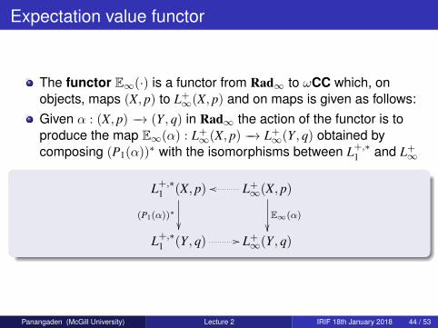
Expectation value functor

The functor E∞(·) is a functor from Rad∞ to ωCC which, onobjects, maps (X, p) to L+

∞(X, p) and on maps is given as follows:Given α : (X, p) −→ (Y, q) in Rad∞ the action of the functor is toproduce the map E∞(α) : L+

∞(X, p) −→ L+∞(Y, q) obtained by

composing (P1(α))∗ with the isomorphisms between L+,∗1 and L+

∞

L+,∗1 (X, p)

(P1(α))∗

��

L+∞(X, p)oo

E∞(α)

��L+,∗

1 (Y, q) // L+∞(Y, q)


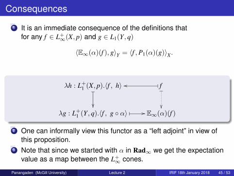
Consequences

1 It is an immediate consequence of the definitions thatfor any f ∈ L+

∞(X, p) and g ∈ L1(Y, q)

〈E∞(α)(f ), g〉Y = 〈f ,P1(α)(g)〉X.

λh : L+1 (X, p).〈f , h〉

_

��

f�oo_

��λg : L+

1 (Y, q).〈f , g ◦ α〉 � // E∞(α)(f )

2 One can informally view this functor as a “left adjoint” in view ofthis proposition.

3 Note that since we started with α in Rad∞ we get the expectationvalue as a map between the L+

∞ cones.


Markov kernels as linear maps

1 Given τ a Markov kernel from (X,Σ) to (Y,Λ), we defineTτ : L+(Y) −→ L+(X), for f ∈ L+(Y), x ∈ X, asTτ (f )(x) =

∫Y f (z)τ(x, dz).

2 This map is well-defined, linear and ω-continuous.3 If we write 1B for the indicator function of the measurable set B we

have that Tτ (1B)(x) = τ(x,B).4 It encodes all the transition probability information


From linear maps to Markov kernels

1 Conversely, any ω-continuous morphism L with L(1Y) ≤ 1X can becast as a Markov kernel by reversing the process on the last slide.

2 The interpretation of L is that L(1B) is a measurable function on Xsuch that L(1B)(x) is the probability of jumping from x to B.


Backwards

1 We can also define an operator onM(X) by using τ the other way.2 We define T̄τ :M(X) −→M(Y), for µ ∈M(X) and B ∈ Λ, as

T̄τ (µ)(B) =∫

X τ(x,B) dµ(x).3 It is easy to show that this map is linear and ω-continuous.


What do they mean?

1 The operator T̄τ transforms measures “forwards in time”; if µ is ameasure on X representing the current state of the system, T̄τ (µ)is the resulting measure on Y after a transition through τ .

2 The operator Tτ may be interpreted as a likelihood transformerwhich propagates information “backwards”, just as we expect frompredicate transformers.

3 Tτ (f )(x) is just the expected value of f after one τ -step given thatone is at x.


Labelled abstract Markov processes

The definitionAn abstract Markov kernel from (X,Σ, p) to (Y,Λ, q) is anω-continuous linear map τ : L+

∞(Y) −→ L+∞(X) with ‖τ‖ ≤ 1.

LAMPSA labelled abstract Markov process on a probability space (X,Σ, p)with a set of labels (or actions) A is a family of abstract Markov kernelsτa : L+

∞(X, p) −→ L+∞(X, p) indexed by elements a of A.


The approximation map

The expectation value functors project a probability space onto anotherone with a possibly coarser σ-algebra.Given an AMP on (X, p) and a map α : (X, p) −→ (Y, q) in Rad∞, wehave the following approximation scheme:

Approximation scheme

L+∞(X, p)

τa // L+∞(X, p)

E∞(α)��

L+∞(Y, q)

α(τa) //

P∞(α)

OO

L+∞(Y, q)


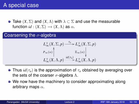
A special case

Take (X,Σ) and (X,Λ) with λ ⊂ Σ and use the measurablefunction id : (X,Σ) −→ (X,Λ) as α.

Coarsening the σ-algebra

L+∞(X,Σ, p)

τa // L+∞(X,Σ, p)

E∞(α)��

L+∞(X,Λ, p)

id(τa) //

P∞(α)

OO

L+∞(X,Λ, p)

Thus id(τa) is the approximation of τa obtained by averaging overthe sets of the coarser σ-algebra Λ.We now have the machinery to consider approximating alongarbitrary maps α.


Conclusions

We have dualized the notion of LMPsWe have made conditional expectation a functorWe have shown how to approximate along a morphismWe can give a logical characterization of bisimulation easilyWe can prove a minimal realization resultWe can construct finite approximants to an abstract Markovprocess.


Documents

A dual view of Markov processes - McGill University School ...prakash/Talks/irif-2.pdf · A dual view of Markov processes Prakash Panangaden1 1School of Computer Science McGill University