A Facility Reliability Problem:Formulation, Properties and Algorithm

Michael Lim1, Mark S. Daskin2,3, Achal Bassamboo3, Sunil Chopra3,2

1 Department of Business Administration,University of Illinois at Urbana–Champaign, Champaign, IL 61820

mlim@illinois.edu

2 Department of Industrial Engineering and Management Sciences,Northwestern University, Evanston, IL 60208

m-daskin@northwestern.edu

3 Department of Managerial Economics and Decision Sciences,Northwestern University, Evanston, IL 60208

a-bassamboo@kellogg.northwestern.edu; s-chopra@kellogg.northwestern.edu

Having a robustly designed supply chain network is one of the most effective ways to hedge

against network disruptions since contingency plans in the event of a disruption are often

significantly limited. In this paper, we study the facility reliability problem: how to design a

reliable supply chain network in the presence of random facility disruptions with the option

of hardening selected facilities. We consider a facility location problem incorporating two

types of facilities, one that is unreliable and another that is reliable (which is not subject

to disruption, but is more expensive). We formulate this as a mixed integer programming

model and develop a Lagrangian Relaxation-based solution algorithm. We derive structural

properties of the problem and show that for some values of the disruption probability, the

problem reduces to the classical uncapacitated fixed charge location problem. In addition, we

show that the proposed solution algorithm is not only capable of solving large-scale problems,

but is also computationally effective.

Keywords : Supply chain disruption; Facility location; Network design

1. Introduction

Each year companies face numerous unexpected events in their supply chains. While com-

panies manage to survive from risks arising at the operational level, many suffer heavily

1

when longer term disruptions impact their supply chain networks. Supply chain disruptions

are entirely different from operational level mishaps (machine failures or short-term supply-

demand imbalances) since they completely block the flow of the network for a significant

amount of time. To hedge against such events, providing a robustly designed network is

of the utmost importance since contingency plans in the event of a major disruption are

significantly limited. Imagine a supply chain network that is designed to minimize the oper-

ational cost without considering any disruption scenarios. Although it may be very difficult

to exactly quantify the damage of supply chain disruptions, it is not impossible to infer the

range of their magnitude. Yet, managers tend to underestimate (if not completely ignore)

the impact of supply chain disruptions, deceived by their small probability of occurrence.

Recent incidents such as the SARS outbreak in Asia or the 9/11 terrorist attacks illustrate

that today’s supply chains operate in a highly uncertain environment and the consequences

of a disruption can be devastating. Motorola and Honda incurred substantial supply chain

delays after the outbreak of SARS (Businessweek, 2003); Ford suffered from part shortages

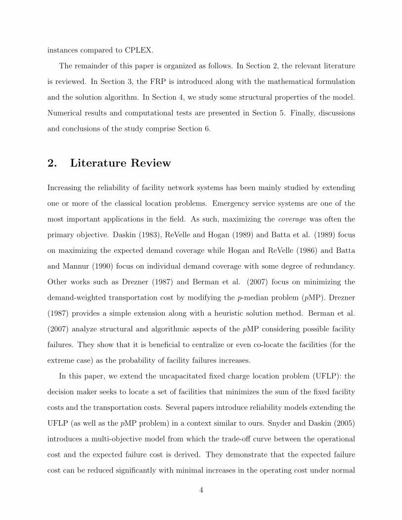
due to the border closing after the 9/11 (Associated Press 2001). According to Swiss Re

(2008), annual losses due to natural hazards have increased dramatically in the past 30

years despite large fluctuations as shown in Figure 1. Not surprisingly, the frequency of

man-made disasters is also on the rise, due to political issues such as military conflicts and

terrorist actions (Coleman 2006, Swiss Re 2009). These examples collectively highlight the

importance of protecting supply chain networks against disruptions.

In this paper, we study facility location and demand assignment decisions incorporating

facility disruptions. Facility location problems have been actively studied spanning numerous

application areas in both public and private sectors (Drezner 2002). However, classical

facility location problems implicitly assume that all facilities are perfectly reliable and derive

the optimal facility locations under this ideal situation. We provide strategies for designing a

robust supply chain network with the option of facility hardening in the presence of random

facility disruptions. Here, not all facilities are assumed to be reliable. We consider two types

2

Total economic losses (estimate) Insured losses

Source: sigma catastrophe database, Swiss Re

Loss burden in USD billions at 2007 prices

1970 1975 1980 1985 1990 1995 2000 2005

250

200

150

100

50

0

Figure 1: Insured losses attributable to natural hazards over the past years

of facilities: regular facilities, hereafter referred to as unreliable facilities, which are subject

to random disruptions, and reliable facilities that are “hardened” as a result of a substantial

investment. We assume reliable facilities are not subject to disruption.

We propose a facility reliability problem (FRP) incorporating the option of facility hard-

ening to hedge against the risk of facility disruptions. The FRP is formulated as a mixed

integer programming model and we propose a Lagrangian relaxation algorithm as a solution

method. By solving the model, we determine the optimal number and locations of both types

of facilities, as well as the assignments of demands to facilities. The main contributions of

our paper are as follows:

(1) By formulating and solving the FRP, we study the relationship between the facility de-

cisions (e.g., facility locations, hardening investment) and some key factors (e.g., disruption

probability and customer demand) in the presence of random disruptions.

(2) We analytically show that under certain conditions, the FRP reduces to one of the well-

studied classical facility location problems.

(3) We propose a Lagrangian Relaxation-based solution algorithm that is fast and effective

for solving the FRP. For the examples analyzed, the proposed algorithm provides near-

optimal solutions quickly (with an optimality gap below 0.1%) and handles larger problem

3

instances compared to CPLEX.

The remainder of this paper is organized as follows. In Section 2, the relevant literature

is reviewed. In Section 3, the FRP is introduced along with the mathematical formulation

and the solution algorithm. In Section 4, we study some structural properties of the model.

Numerical results and computational tests are presented in Section 5. Finally, discussions

and conclusions of the study comprise Section 6.

2. Literature Review

Increasing the reliability of facility network systems has been mainly studied by extending

one or more of the classical location problems. Emergency service systems are one of the

most important applications in the field. As such, maximizing the coverage was often the

primary objective. Daskin (1983), ReVelle and Hogan (1989) and Batta et al. (1989) focus

on maximizing the expected demand coverage while Hogan and ReVelle (1986) and Batta

and Mannur (1990) focus on individual demand coverage with some degree of redundancy.

Other works such as Drezner (1987) and Berman et al. (2007) focus on minimizing the

demand-weighted transportation cost by modifying the p-median problem (pMP). Drezner

(1987) provides a simple extension along with a heuristic solution method. Berman et al.

(2007) analyze structural and algorithmic aspects of the pMP considering possible facility

failures. They show that it is beneficial to centralize or even co-locate the facilities (for the

extreme case) as the probability of facility failures increases.

In this paper, we extend the uncapacitated fixed charge location problem (UFLP): the

decision maker seeks to locate a set of facilities that minimizes the sum of the fixed facility

costs and the transportation costs. Several papers introduce reliability models extending the

UFLP (as well as the pMP problem) in a context similar to ours. Snyder and Daskin (2005)

introduces a multi-objective model from which the trade-off curve between the operational

cost and the expected failure cost is derived. They demonstrate that the expected failure

cost can be reduced significantly with minimal increases in the operating cost under normal

4

circumstances. In Snyder and Daskin (2006), the concept of stochastic p-robustness is intro-

duced where the relative regret is always less than p for any possible scenario. With this, the

decision maker can minimize the total cost at a desired level of system performance. Zhan et

al. (2007) and Cui et al. (2008) point out that site-specific failure probabilities may impact

the choice of facility locations significantly and extend the literature by incorporating such

characteristics. Zhan et al. (2007) provide a genetic algorithm and Cui et al. (2008) provide

a Lagrangian relaxation algorithm as a solution method. We also allow site-specific failure

probabilities in our model.

Our paper differs from these papers in two ways. First, we consider an option of “facility

hardening;” hence another set of decisions is made. The notion of facility hardening implies

various protection plans ranging from physical facility protection to exogenous outsourcing

contracts. Using a mixture of reliable and unreliable facilities is akin to problems studied

in Tomlin (2006) and Chopra et al. (2007) in the supplier risk management literature.

These studies show that using reliable facilities can be valuable (even though they are more

expensive) and effective in hedging against disruption risks. Second, we require each demand

to have a “backup assignment” to a reliable facility whereas the earlier research allows a

cascading strategy to the next available facility. Our approach significantly reduces the

operational complexity of a firm since the hierarchical structure between the facilities is

clear. Also, our approach allows us to study the problem analytically. A close similarity

can also be found to Pirkul and Schilling (1988) and Pirkul (1989) where they designate

the primary and secondary facilities for each demand node. However, our approach differs

from these papers in a number of ways: we consider facility hardening decisions and provide

structural properties of the model.

Church and Scaparra (2007) and Scaparra and Church (2008) extend the pMP to the

case in which the decision maker tries to find the optimal number of facilities q to protect

to hedge against a predetermined number, r, of facility disruptions. However, the facility

disruption in these papers is caused by an intelligent adversary who tries to maximize the

5

damage to the system. The objective of the model differs from the objective in our model -

their model minimizes against the worst case scenario rather than the expected failure case

- thus the protection policy significantly differs as a result.

Finally, we note that the FRP is also formulated in a continuous model in Lim et al.

(2009). In that paper, the focus is on deriving managerial implications. The discrete model

and the continuous model are compared using a case example. For more details on reliability

considerations in facility location models, please refer to Snyder et al. (2006).

3. The Facility Reliability Model (FRP)

3.1 Problem Formulation

The facility reliability problem (FRP) extends the uncapacitated fixed charge location prob-

lem (UFLP) taking random facility disruptions into account. The objective of the problem

is to minimize the total facility fixed cost and the expected transportation cost by properly

locating reliable and unreliable facilities. We assume that each node j ∈ N , where N is a

set of all nodes, is a demand node and a candidate facility site. At each node, we may locate

either an unreliable facility at a cost of fUj which may fail with probability qj (0 < qj < 1) or

a reliable facility at a cost of fRj that does not fail. For the reliability premium, we assume

fRj > fUj . In keeping with the UFLP, the decision maker determines the optimal number and

location of both types of facilities while serving all demand nodes with probability 1 utilizing

primary and backup assignments. A demand node i is served primarily by “any” type of

facility as a primary assignment and by the closest “reliable” facility as a backup assignment

in case the primarily assigned facility fails. The transportation cost per unit demand from a

demand at node i to a facility at node j is given by dPij and dBij for a primary assignment and

backup assignment, respectively. We allow dBij ≥ dPij to capture the penalty cost (emergency

cost) associated with utilizing the backup source. When the closest facility from a certain

demand node is a reliable facility, the primary assignment and the backup assignment are

6

identical and we assume the unit transportation cost is always dPij. To incorporate this into

our model, we introduce dSij (= dBij − dPij ≥ 0) as the unit savings that will be used to adjust

the objective function by subtracting the over-levied travel cost as a savings. Facilities are

assumed to have ample capacity to cover all the demands assigned to them and each node i

has a demand of ℎi. The complete notation for the FRP is summarized below.

Inputs:

N = set of all nodes

ℎi = demand at node i ∈ N

fUj = fixed cost of locating an unreliable facility which is subject to failure at node j ∈ N

fRj = fixed cost of locating a reliable facility which does not fail at node j ∈ N

qj = probability that an unreliable facility at j ∈ N will be in the failure state

dPij = unit transportation cost for a primary assignment from demand node i ∈ N to afacility at j ∈ N

dBij = unit transportation cost for a backup assignment from demand node i ∈ N to areliable facility at j ∈ N

dSij = unit savings cost when demand node i ∈ N is assigned to a reliable facility at j ∈ Nas both the primary and backup facility

Decision Variables:

XUj = 1 if an unreliable facility is located at candidate site j; 0 if not

XRj = 1 if a reliable facility is located at candidate site j; 0 if not

Y Pij = 1 if demands at i are assigned to a facility at j as the primary site; 0 if not

Y Bij = 1 if demands at i are assigned to a facility at j as the backup site; 0 if not

Y Sij = 1 if demands at i are assigned to a facility at j as the primary and backup site; 0 if

not.

7

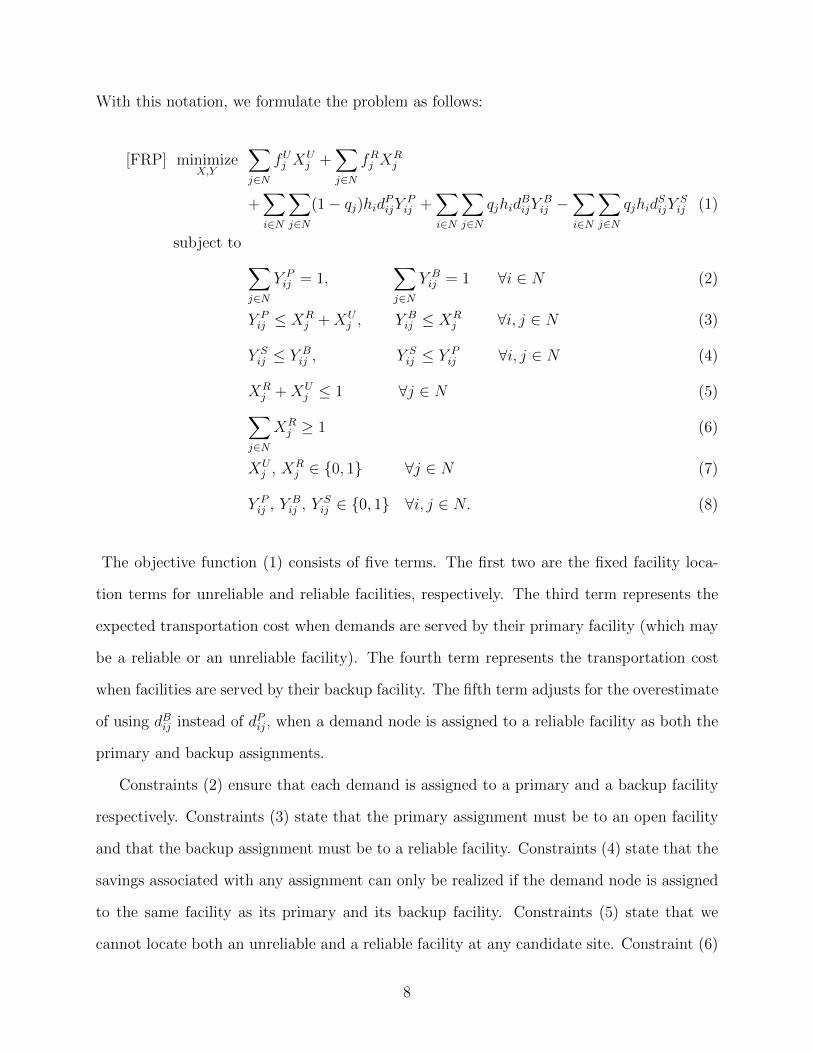
With this notation, we formulate the problem as follows:

[FRP] minimizeX,Y

∑j∈N

fUj XUj +

∑j∈N

fRj XRj

+∑i∈N

∑j∈N

(1− qj)ℎidPijY Pij +

∑i∈N

∑j∈N

qjℎidBijY

Bij −

∑i∈N

∑j∈N

qjℎidSijY

Sij (1)

subject to ∑j∈N

Y Pij = 1,

∑j∈N

Y Bij = 1 ∀i ∈ N (2)

Y Pij ≤ XR

j +XUj , Y B

ij ≤ XRj ∀i, j ∈ N (3)

Y Sij ≤ Y B

ij , Y Sij ≤ Y P

ij ∀i, j ∈ N (4)

XRj +XU

j ≤ 1 ∀j ∈ N (5)∑j∈N

XRj ≥ 1 (6)

XUj , X

Rj ∈ {0, 1} ∀j ∈ N (7)

Y Pij , Y

Bij , Y

Sij ∈ {0, 1} ∀i, j ∈ N. (8)

The objective function (1) consists of five terms. The first two are the fixed facility loca-

tion terms for unreliable and reliable facilities, respectively. The third term represents the

expected transportation cost when demands are served by their primary facility (which may

be a reliable or an unreliable facility). The fourth term represents the transportation cost

when facilities are served by their backup facility. The fifth term adjusts for the overestimate

of using dBij instead of dPij, when a demand node is assigned to a reliable facility as both the

primary and backup assignments.

Constraints (2) ensure that each demand is assigned to a primary and a backup facility

respectively. Constraints (3) state that the primary assignment must be to an open facility

and that the backup assignment must be to a reliable facility. Constraints (4) state that the

savings associated with any assignment can only be realized if the demand node is assigned

to the same facility as its primary and its backup facility. Constraints (5) state that we

cannot locate both an unreliable and a reliable facility at any candidate site. Constraint (6)

8

ensures that we locate at least one reliable facility. Technically, this is a redundant constraint

as it is implied by (2) and (3). However, we keep this constraint for later use. Constraints

(8) are the integrality constraints.

3.2 Solution Method: Lagrangian Relaxation Algorithm

The FRP can be solved using a standard optimization solver such as CPLEX, but the compu-

tation time and resource usage grows drastically as the size of the problem increases. Thus,

to solve this problem effectively, we develop an algorithm based on Lagrangian relaxation

(LR). A comparison between CPLEX and the LR algorithm is in §5.2.

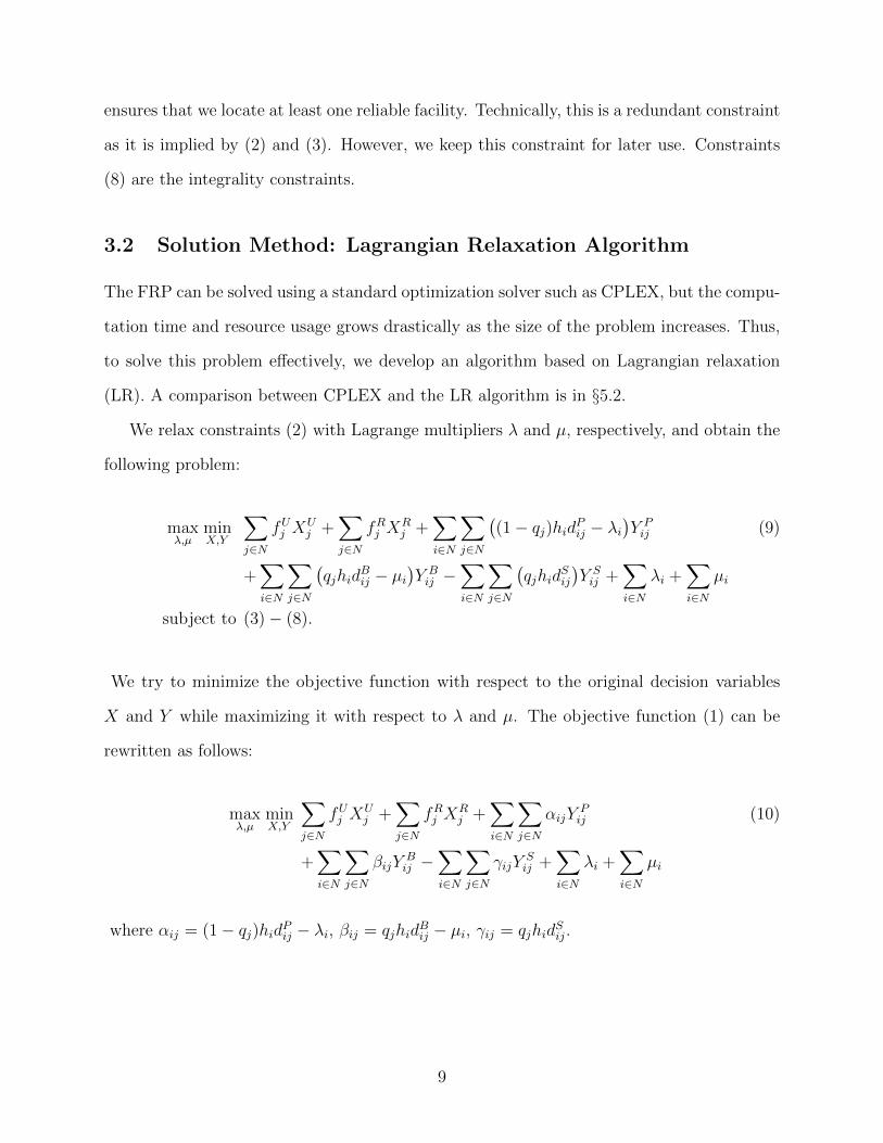
We relax constraints (2) with Lagrange multipliers � and �, respectively, and obtain the

following problem:

max�,�

minX,Y

∑j∈N

fUj XUj +

∑j∈N

fRj XRj +

∑i∈N

∑j∈N

((1− qj)ℎidPij − �i

)Y Pij (9)

+∑i∈N

∑j∈N

(qjℎid

Bij − �i

)Y Bij −

∑i∈N

∑j∈N

(qjℎid

Sij

)Y Sij +

∑i∈N

�i +∑i∈N

�i

subject to (3)− (8).

We try to minimize the objective function with respect to the original decision variables

X and Y while maximizing it with respect to � and �. The objective function (1) can be

rewritten as follows:

max�,�

minX,Y

∑j∈N

fUj XUj +

∑j∈N

fRj XRj +

∑i∈N

∑j∈N

�ijYPij (10)

+∑i∈N

∑j∈N

�ijYBij −

∑i∈N

∑j∈N

ijYSij +

∑i∈N

�i +∑i∈N

�i

where �ij = (1− qj)ℎidPij − �i, �ij = qjℎidBij − �i, ij = qjℎid

Sij.

9

3.2.1 Algorithm Outline

The Lagrangian relaxation algorithm improves the lower and upper bound by constantly

adjusting the Lagrange multipliers until either the gap between the lower and upper bound

goes below a prespecified level or another termination criterion is attained. Notice that

relaxing (2) allows the solution to be feasible even without having any reliable facility if (6)

did not exist. We incorporate these constraints into the procedure for solving the FRP by

using the algorithm below.

Initialize Lagrange multipliersWhile (Termination condition not met) Do{

Increment iteration counterCompute the lower boundCompute the upper bound(Optional) Local improvementCheck termination conditionUpdate Lagrange multipliers

}

Now we present each step of the algorithm in detail.

3.2.2 Computation of the Lower Bound

We compute the lower bound first. For fixed values of the Lagrange multipliers � and �, (10)

provides a lower bound on the objective function (1). We solve (10) by using the following procedure:

Step 0. Initialize all decision variables, XUj , X

Rj , Y

Pij , Y

Bij , Y

Sij , to 0.

Step 1. Determine the value of locating an unreliable facility (i.e., setting XUj = 1) at site j

for every such site. This will allow us to set Y Pij = 1 by the first constraint of (3) if doing so is

advantageous to the Lagrangian objective function (10), which is minimized with respect to the

original decision variables. We will want to set Y Pij = 1, if �ij = (1 − qj)ℎidPij − �i < 0. Thus,

the value of setting XPj = 1, exclusive of the fixed facility costs, is V U

j =∑

i∈N min(0, �ij) =∑i∈N min(0, (1− qj)ℎidPij − �i).

Step 2. Determine the value of locating a reliable facility at a node (i.e., setting XRj = 1) in a

similar manner. This is somewhat more complicated than step 1 since doing so impacts constraints,

(3), and by implication constraints (4). Once we set XRj = 1, we will want to set Y P

ij , Y Bij and Y S

ij

10

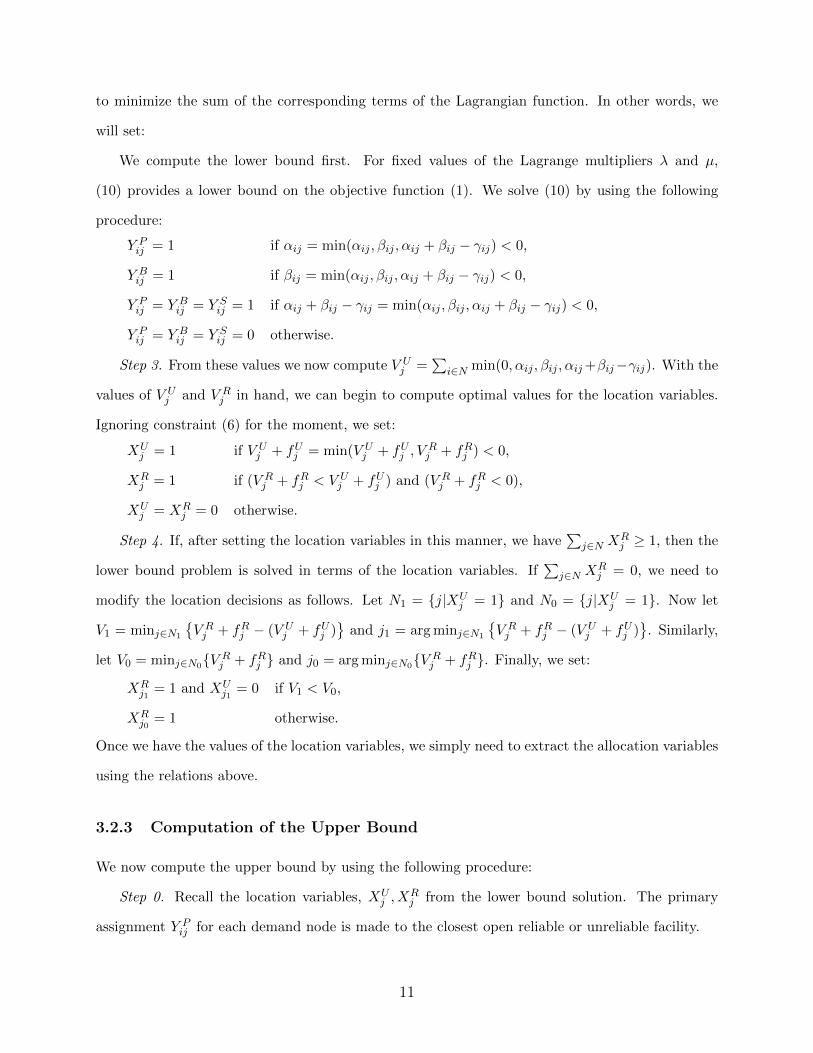
to minimize the sum of the corresponding terms of the Lagrangian function. In other words, we

will set:

We compute the lower bound first. For fixed values of the Lagrange multipliers � and �,

(10) provides a lower bound on the objective function (1). We solve (10) by using the following

procedure:

Y Pij = 1 if �ij = min(�ij , �ij , �ij + �ij − ij) < 0,

Y Bij = 1 if �ij = min(�ij , �ij , �ij + �ij − ij) < 0,

Y Pij = Y B

ij = Y Sij = 1 if �ij + �ij − ij = min(�ij , �ij , �ij + �ij − ij) < 0,

Y Pij = Y B

ij = Y Sij = 0 otherwise.

Step 3. From these values we now compute V Uj =

∑i∈N min(0, �ij , �ij , �ij+�ij− ij). With the

values of V Uj and V R

j in hand, we can begin to compute optimal values for the location variables.

Ignoring constraint (6) for the moment, we set:

XUj = 1 if V U

j + fUj = min(V Uj + fUj , V

Rj + fRj ) < 0,

XRj = 1 if (V R

j + fRj < V Uj + fUj ) and (V R

j + fRj < 0),

XUj = XR

j = 0 otherwise.

Step 4. If, after setting the location variables in this manner, we have∑

j∈N XRj ≥ 1, then the

lower bound problem is solved in terms of the location variables. If∑

j∈N XRj = 0, we need to

modify the location decisions as follows. Let N1 = {j∣XUj = 1} and N0 = {j∣XU

j = 1}. Now let

V1 = minj∈N1

{V Rj + fRj − (V U

j + fUj )}

and j1 = arg minj∈N1

{V Rj + fRj − (V U

j + fUj )}

. Similarly,

let V0 = minj∈N0{V Rj + fRj } and j0 = arg minj∈N0{V R

j + fRj }. Finally, we set:

XRj1

= 1 and XUj1

= 0 if V1 < V0,

XRj0

= 1 otherwise.

Once we have the values of the location variables, we simply need to extract the allocation variables

using the relations above.

3.2.3 Computation of the Upper Bound

We now compute the upper bound by using the following procedure:

Step 0. Recall the location variables, XUj , X

Rj from the lower bound solution. The primary

assignment Y Pij for each demand node is made to the closest open reliable or unreliable facility.

11

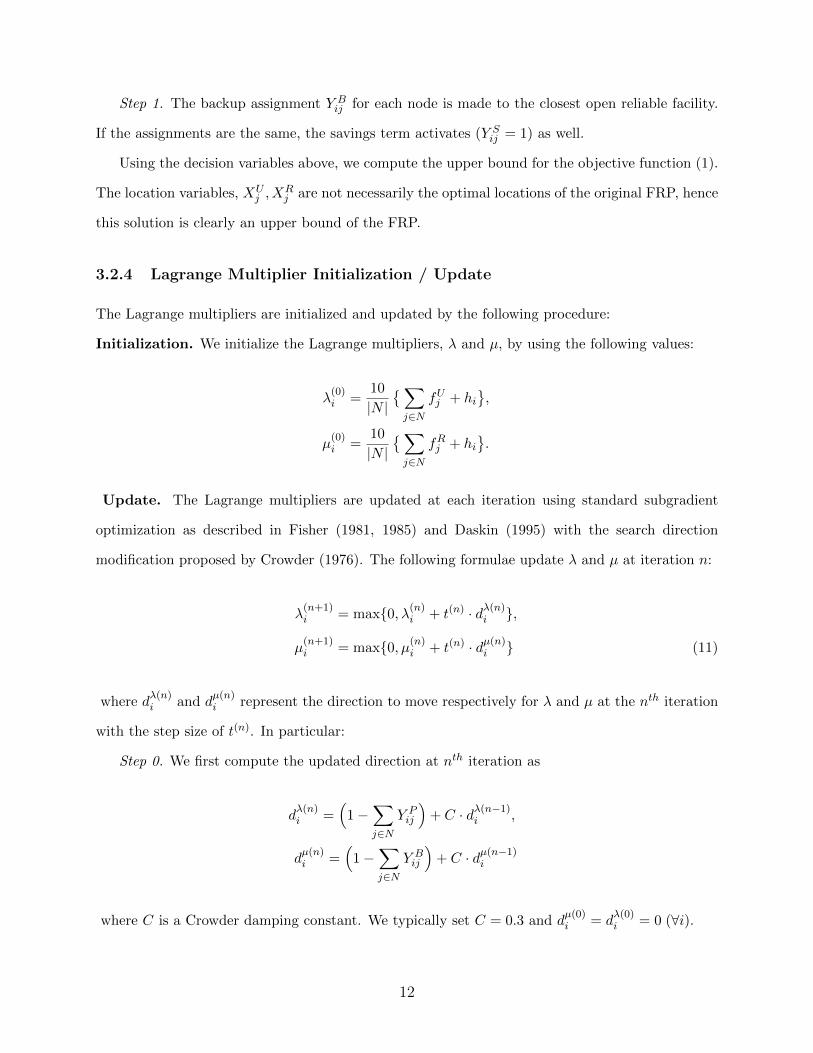
Step 1. The backup assignment Y Bij for each node is made to the closest open reliable facility.

If the assignments are the same, the savings term activates (Y Sij = 1) as well.

Using the decision variables above, we compute the upper bound for the objective function (1).

The location variables, XUj , X

Rj are not necessarily the optimal locations of the original FRP, hence

this solution is clearly an upper bound of the FRP.

3.2.4 Lagrange Multiplier Initialization / Update

The Lagrange multipliers are initialized and updated by the following procedure:

Initialization. We initialize the Lagrange multipliers, � and �, by using the following values:

�(0)i =

10

∣N ∣{∑j∈N

fUj + ℎi},

�(0)i =

10

∣N ∣{∑j∈N

fRj + ℎi}.

Update. The Lagrange multipliers are updated at each iteration using standard subgradient

optimization as described in Fisher (1981, 1985) and Daskin (1995) with the search direction

modification proposed by Crowder (1976). The following formulae update � and � at iteration n:

�(n+1)i = max{0, �(n)

i + t(n) ⋅ d�(n)i },

�(n+1)i = max{0, �(n)

i + t(n) ⋅ d�(n)i } (11)

where d�(n)i and d

�(n)i represent the direction to move respectively for � and � at the ntℎ iteration

with the step size of t(n). In particular:

Step 0. We first compute the updated direction at ntℎ iteration as

d�(n)i =

(1−

∑j∈N

Y Pij

)+ C ⋅ d�(n−1)

i ,

d�(n)i =

(1−

∑j∈N

Y Bij

)+ C ⋅ d�(n−1)

i

where C is a Crowder damping constant. We typically set C = 0.3 and d�(0)i = d

�(0)i = 0 (∀i).

12

Step 1. We next compute the stepsize t(n) as

t(n) = �(n) (UB − ℒ(n))∑i∈N

(d�(n)i

)2+∑

i∈N(d�(n)i

)2where �(n) is a constant at iteration n, initialized to 2.0 and halved when 24 consecutive iterations

fail to improve the lower bound. UB denotes the best (lowest) known upper bound through iteration

n and ℒ(n) denotes the value of the lower bound found at iteration n.

Step 2. Finally, we update � and � by using (11) above.

3.2.5 Termination Conditions

The algorithm terminates when any of the following conditions are met:

1. Optimality Gap: When the gap between the lower and upper bound gets close to zero; i.e.,

(UB−ℒ(n))

ℒ(n) < � where we typically prespecified the tolerance value � to 0.00001.

2. Maximum Iteration: When the iteration number reaches a prespecified number; i.e., n >

nmax where we typically set the iteration limit to 10,000.

3. Stepsize Constant: When the stepsize constant �(n) gets close to zero; i.e., �(n) < �min

where we typically set the stepsize constant limit to 0.0001.

3.2.6 (Optional) Local Improvements

Four local heuristic improvement (LHI) algorithms can be applied to the solution to enhance the

performance of the algorithm. These heuristics typically work well in the early iterations until the

solution becomes stable.

LHI 1. We consider changing an unreliable site to a reliable site. This incurs the incremental

hardening cost, but may reduce the transport costs to some nodes sufficiently since the customers

at those nodes no longer need to travel to a more remote backup or reliable facility in the event

that the facility at node j fails. Also, this hardened site may reduce the backup transportation cost

for some demand nodes which had been assigned to a more remote backup facility.

LHI 2. Similarly, we consider changing a reliable facility into an unreliable facility, provided

there is at least one other reliable facility in the system. These two improvement algorithms are

13

very fast since, for each facility, there is at most one other objective function evaluation.

LHI 3. We consider an exchange algorithm, in which each unreliable facility in turn is removed

and replaced by an unreliable facility at a node that does not have a facility.

LHI 4. Lastly, we consider an exchange algorithm for the reliable facilities. The last two

improvement algorithms are more intensive as they require O(∣J ∣) objective function evaluations

for every facility, where J is the set of candidate locations.

4. Structural Properties

In this section, we develop important structural properties of the facility reliability problem (FRP).

We show that for extreme values of the disruption probability, the FRP is reducible to the unca-

pacitated fixed charge location problem (UFLP). Consequently, we derive threshold bounds on the

disruption probability that satisfy such conditions. We begin with the case when the disruption

probabilities are large.

Theorem 1. There exists a threshold disruption probability qtℎ (< 1) for the FRP such that if all

qj ≥ qtℎ, then it is optimal to deploy only reliable facilities. Further, the optimal location of these

facilities coincides with the optimal solution to the UFLP with facility costs fRj and distances dPij.

Proof. Let q be the disruption probability vector. Consider a feasible solution S : (XU ,XR,YP ,YB,YS)

which contains at least one unreliable facility where vectors XU ,XR and YP ,YB,YS represent the

optimal locations and assignments for such a solution, respectively. Now consider another solution

S : (0,XR,YB,YB,YB). Denoting ZFRP(S) as the total cost of the FRP with the configuration

S, we know the following holds for any q:

ZFRP(XU ,XR,YP ,YB,YS)− ZFRP(0,XR,YB,YB,YB)

=∑j∈N

fUj XUj +

∑i∈N

∑j∈N

(1− qj)ℎidPijY Pij +

∑i∈N

∑j∈N

qjℎidBijY

Bij −

∑i∈N

∑j∈N

qjℎidSijY

Sij −

∑i∈N

∑j∈N

ℎidPijY

Bij

=∑j∈N

fUj XUj +

∑i∈N

∑j∈N

qjℎi(dBij − dPij)(Y B

ij − Y Sij )−

∑i∈N

∑j∈N

(1− qj)ℎidPij(Y Bij − Y P

ij )

≥∑j∈N

fUj XUj −

∑i∈N

∑j∈N

(1− qj)ℎidPij(Y Bij − Y P

ij ).

14

The inequality holds since Y Bij ≥ Y S

ij and dBij ≥ dPij . Since∑

j∈N fUj X

Uj > 0, we can find a q

that satisfies ZFRP(XU ,XR,YP ,YB,YS) ≥ ZFRP(0,XR,YB,YB,YB) for qj ’s that are sufficiently

close to 1. That is, for a given configuration S, there always exists a threshold probability q(S)

such that if qj ≥ q(S) ∀j, then it is optimal to use only reliable facilities. Then, we can find a

threshold probability qtℎ by taking the supremum over all possible q(S)’s; i.e., supS∈Ω

q(S) =: qtℎ where

Ω represents all possible configurations for a given network. There is only finite number of possible

configurations in Ω, thus we know that qtℎ < 1. Therefore, we conclude that if all qj ≥ qtℎ ∀j, then

it is optimal to deploy only reliable facilities.

Now, let ZUFLP(XR,YB) be the total cost for the UFLP with the facility cost of fRj and the

distance of dPij where XR,YB are the location and assignment vectors. Note that this is equivalent

to ZFRP(0,XR,YB,YB,YB). Then, it follows that

ZFRP(0,XR,YB,YB,YB) = ZUFLP(XR,YB)

≥ ZUFLP(X∗,Y∗) = ZFRP(0,X∗,Y∗,Y∗,Y∗) (12)

where X∗ and Y∗ is the optimal solution to the UFLP with the facility cost of fRj and the distance

of dPij . From the first statement, we know that all facilities should be hardened if qj ≥ qtℎ and

under this condition, (12) implies that the optimal solution of the FRP coincides with the optimal

solution to the UFLP with facility costs fRj and distances dPij . ■

In the proof of Theorem 1, we notice from (12) that q satisfies ZFRP(XU ,XR,YP ,YB,YS) ≥

ZFRP(0,XR,YB,YB,YB) if∑

j∈N fUj X

Uj −

∑i∈N

∑j∈N (1− qj)ℎidPij(Y B

ij − Y Pij ) ≥ 0. We can see

that the worst bound would correspond to the case where all qj ’s are equal. A q(S) = qj that

satisfies this relationship for configuration S can then be derived as

∑j∈N

fUj XUj − (1− q(S))

∑i∈N

∑j∈N

ℎidPij(Y

Bij − Y P

ij ) ≥ 0

=⇒ q(S) ≥ 1−∑

j∈N fUj X

Uj∑

i∈N∑

j∈N ℎidPij(Y

Bij − Y P

ij ). (13)

Since supS∈Ω

q(S) =: qtℎ, we construct an upper bound on qtℎ in the following corollary.

Corollary 1. The threshold disruption probability qtℎ is bounded above (upper bound) by the value

15

of max[

0, 1− fUmin∑i∈N ℎi(dPmax i−dPmin i)

], where dPmax i = max

j{dPij} and dPmin i = min

j{dPij}.

Proof. Note that Y Bij is the backup assignment to the closest reliable facility from demand i while

Y Pij is to the closest facility (of either type) to demand i. Thus, for every i, 0 ≤ ℎi

(∑j∈N d

Pij(Y

Bij −

Y Pij ))≤ ℎi

(dPmax i − dPmin i

)holds. Consequently, 0 ≤

∑i∈N

∑j∈N ℎid

Pij(Y

Bij − Y P

ij )

≤∑

i∈N ℎi(dPmax i − dPmin i

)holds. Hence, it follows that

1∑i∈N ℎi

(dPmax i − dPmin i

) ≤ 1∑i∈N

∑j∈N ℎid

Pij(Y

Bij − Y P

ij )

=⇒ fUmin∑i∈N ℎi

(dPmax i − dPmin i

) ≤ ∑j∈N f

Uj X

Uj∑

i∈N∑

j∈N ℎidPij(Y

Bij − Y P

ij )

=⇒ 1−∑

j∈N fUj X

Uj∑

i∈N∑

j∈N ℎidPij(Y

Bij − Y P

ij )≤ 1− fUmin∑

i∈N ℎi(dPmax i − dPmin i

) (14)

where fUmin represents the unreliable facility with the lowest fixed cost. By (13) and (14), we have

an upper bound on qtℎ in 1 − fUmin∑i∈N ℎi

(dPmax i−dPmin i

) . Note that this bound may become negative

when the fixed cost is much greater than transportation cost (since the FRP requires having at

least one reliable facility), hence we take the maximum between 0 and 1 − fUmin∑i∈N ℎi(dPmax i−dPmin i)

.

■

To summarize, the above theorem and corollary suggest that when the disruption probabilities

are larger than the threshold (qj ≥ qtℎ), it is optimal to have only reliable facilities. Once it

becomes advantageous to harden all the facilities, the FRP is solved in a risk-free environment,

thus its optimal facility location becomes identical to that of the UFLP.

Next, we consider the case when the disruption probabilities are very small.

Theorem 2. If the facility hardening costs are identical for all sites (fRj − fUj = � ∀j), there exists

a threshold disruption probability qtℎ

(> 0) for the FRP such that if all qj ≤ qtℎ, then it is optimal

to harden exactly one of the facilities. Further, the optimal locations of the facilities (including both

reliable and unreliable) coincide with the optimal locations to the UFLP with facility costs fUj and

distances dPij.

Proof. Consider a feasible solution S : (XU ,XR,YP ,YB,YS) which contains at least two reliable

facilities. Say∑

j∈N XRj is � (≥ 2). Also, consider another feasible solution which converts all the

16

reliable facilities from S into unreliable facilities except for one site. (Recall, the smallest number of

reliable facilities is one for the FRP.) More precisely, let S : (XU , XR, YP , YB, YS) be as follows:

XR

= a unit vector with ktℎ element being 1 where k ∈ {j ∣XRj = 1}

(convert all the facilities from XR to unreliable ones except for one)

XU

= XU + XR − XR

(existing unreliable facilities, XU , plus the converted facilities from

XU )

YP

= Each demand is assigned to its closest facility; i.e., YP

= YP

YB

= All demands are assigned to the ktℎ facility; i.e., Y Bij = 1 if j = k; 0 if not

YS

= Demands whose primary and backup assignments are identical; i.e., Y Sij = 1 if j =

k; 0 if not, hence YS

= YB.

Then, for any disruption probability q, we know the following:

ZFRP(XU,XR,YP,YB,YS)− ZFRP(XU, X

R, Y

P, Y

B, Y

S)

=∑j∈N

fUj (XUj −XU

j ) +∑j∈N

fRj (XRj −XR

j ) +∑i∈N

∑j∈N

qjℎidBij(Y

Bij − Y B

ij )−∑i∈N

∑j∈N

qjℎidSij (Y S

ij −Y Sij )

=(�− 1)� +∑i∈N

∑j∈N

qjℎidBij (Y B

ij −Y Bij )−

∑i∈N

∑j∈N

qjℎidSij(Y

Sij −Y S

ij ).

Since � > 0, we find a q that satisfies ZFRP(XU,XR,YP,YB,YS) ≥ ZFRP(XU, X

R, Y

P, Y

B, Y

S)

for qj ’s that are sufficiently close to 0. That is, for a given configuration S, there always exists a

threshold probability q1(S) such that if qj ≤ q

1(S) ∀j, then it is optimal to harden exactly one of

the facilities.

Now, let ZUFLP(X, Y) be the total cost of solving a UFLP with facility costs fUj and distances

dPij where X = XU

+ XR

and Y = YP

. Then, we can find a q that satisfies the following:

ZFRP(XU, X

R, Y

P, Y

B, Y

S)

= ZUFLP(X, Y) + � −∑i∈N

∑j∈N

qjℎi [ dPij YPij − dBij Y B

ij + dSij YSij ]

≥ ZUFLP(X∗, Y∗) + � −

∑i∈N

∑j∈N

qjℎi [ dPij YP∗ij − dBij Y B∗

ij + dSij YS∗ij ]

= ZFRP(XU∗, X

R∗, Y

P∗, Y

B∗, Y

S∗) (15)

17

where X∗

and Y∗

is the optimal solution to the UFLP with facility costs fUj and distances dPij .

The configuration (XU∗, X

R∗, Y

P∗, Y

B∗, Y

S∗) represents the optimal solution to the FRP with one

facility hardened from the configuration (X∗, Y∗) for the UFLP. Note that these configurations

have exactly the same facility locations. Hence, there exists a threshold probability q2(S) such that

if qj ≤ q2(S) ∀j, then the optimal location for the FRP coincides with the optimal location for the

UFLP.

From the first and second statements, let q(S) = q1(S) ∪ q

2(S). Then, we can find a threshold

probability qtℎ

as infS∈Ω

q(S) =: qtℎ

for any given configuration S ∈ Ω. There are only a finite number

of possible configurations in Ω, thus we know that qtℎ> 0. Therefore, if qj ≤ qtℎ, then it is optimal

to have only one reliable facility, and (15) implies that the optimal locations for the FRP coincide

with the optimal locations for the UFLP with facility costs fRj and distances dPij . ■

After solving the UFLP, we can decide which facility to harden by solving a suitably modified

1-median location problem. Since the facility hardening cost is constant, we find one facility to

harden from among the opened facilities which minimizes the total transportation cost for the case

when disruption occurs. Letting N ′ be the set which contains all the opened sites from Theorem

2, we summarize this in the following corollary.

Corollary 2. The one facility that should be hardened from the UFLP in Theorem 2 can be deter-

mined by solving the following 1-median location problem:

mininizeX,Y

∑i∈N

∑j∈N ′

ℎid′ijY

Bij (16)

where d′ij = qjdPij if facility j is the closest to demand i; qjd

Bij if not

subject to∑j∈N ′

Y Bij = 1 ∀i ∈ N

∑j∈N ′

XRj = 1

Y Bij ≤ XR

j ∀i ∈ N, ∀j ∈ N ′

Y Bij ∈ {0, 1} ∀i ∈ N, ∀j ∈ N ′, XR

j ∈ {0, 1} ∀j ∈ N ′.

Proof. Recall that the optimal solution of XU ,YP from Theorem 2 is a minimizer of the UFLP,∑j∈N f

Uj X

Uj +

∑i∈N

∑j∈N ℎid

PijY

Pij . This minimizes

∑j∈N f

Uj X

Uj +

∑i∈N

∑j∈N (1− qj)ℎidPijY P

ij

18

as well under qj ≤ qtℎ

. Also, the facility hardening cost,∑

j∈N ′ fRj XRj = �, is a constant. From

Theorem 2, we know qj ≤ qtℎ so that it is optimal to decide XU ,YP first and then decide XR,YB

(with fixed XU ,YP ). Hence, reducing the solution set of XR,YB from N to N ′ does not affect the

solution. With the definition of d′ij , the objective function∑

i∈N∑

j∈N ′ ℎid′ijY

Bij is equivalent to∑

i∈N∑

j∈N qjℎi(dBijY

Bij − dSijY S

ij ) and this is minimized by (16). Note that the objective function

of FRP, (1), is the sum of these terms, thus the solution of (16) provides the global optimum. ■

Finally, we note that deriving a simple lower bound on qtℎ

is difficult because of the condition on

q2(S). The second and third equation from (15) have different facility configurations and this makes

it analytically challenging to calculate a good closed form bound on the disruption probability.

5. Numerical Results

5.1 Case Example

Case Input. To analyze the problem and to gain insights from the model, we employ a data

set of 263 nodes representing the largest cities in the contiguous 48 states in the United States.

The disruption probability qj was assumed to occur independently and was randomly generated

from U ∼ [0.025, 0.075]. The cost of an unreliable facility fUj was determined by a fixed cost plus a

variable cost which was a function of the population in each node; specifically, fUj = 500, 000+1.7ℎj .

The hardening cost for each site was determined as a linear function of the disruption probability;

i.e., �j = (fRj − fUj ) = 5, 000, 000 qj . Thus, cities facing higher disruption probabilities will be

more costly to harden. In this setting, the hardening cost was roughly 25% of the fixed cost of

the unreliable facility on average. The distance between any two cities was calculated as the great

circle distance based on the longitude and latitude of the cities. Then, we multiplied the distance by

c = 0.002 to get the transportation cost per unit distance, dPij . For simplicity, the backup traveling

cost was set to dBij = 1.25 dPij .

Solution. The solution algorithm was coded in C++ and was run on an IBM workstation with

2.4GHz quad core processor and 9GB of virtual RAM (4GB of physical memory and 5GB of swap

space). A solution with 0.0006% optimality gap (the percentage difference between the upper bound

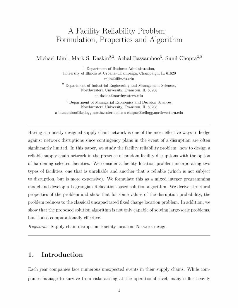
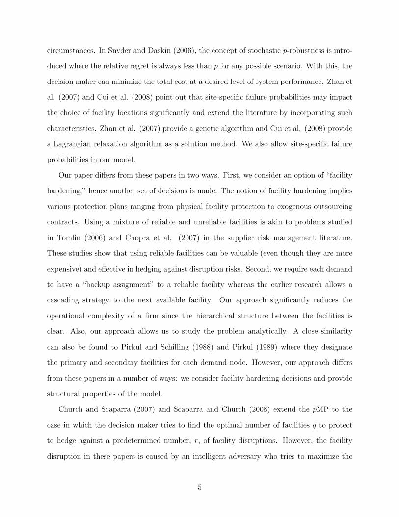
and lower bound) was found in 10.21 second after 304 iterations. Figure 2 shows the locations of the

19

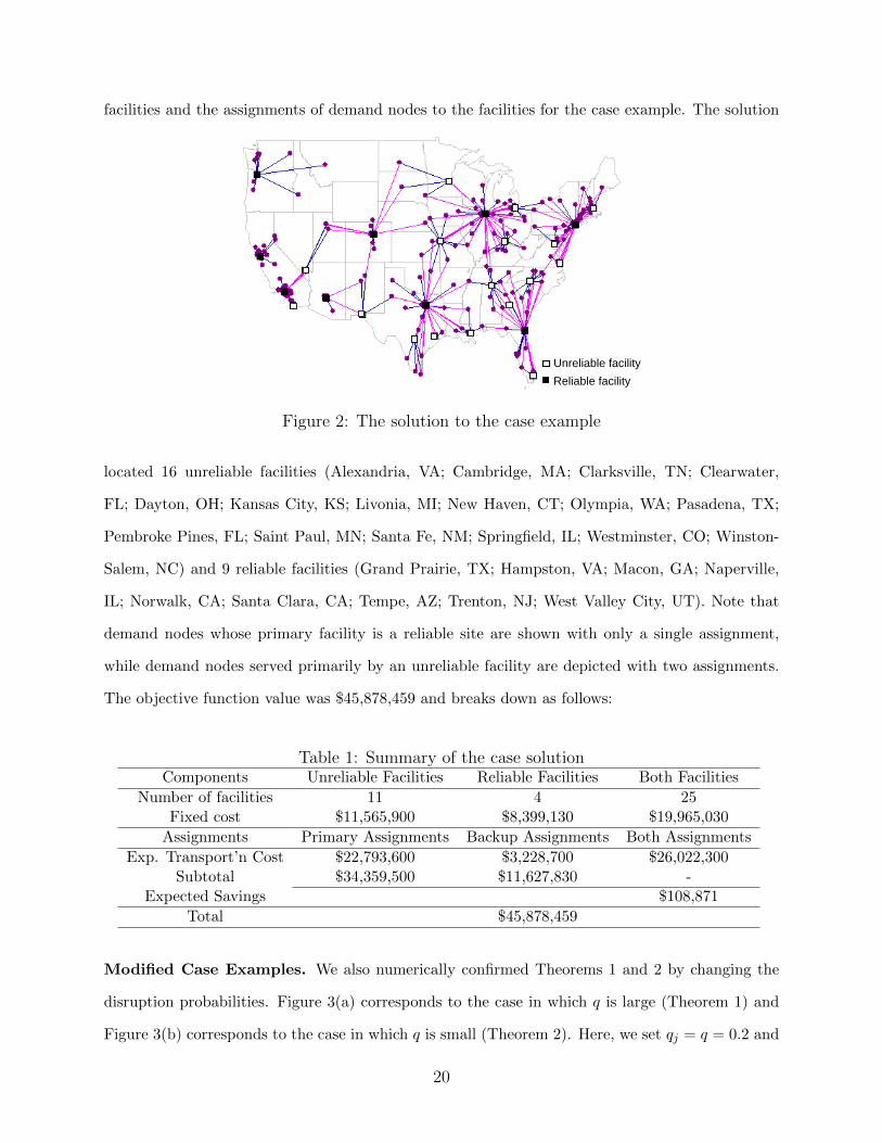
facilities and the assignments of demand nodes to the facilities for the case example. The solution

Unreliable facilityReliable facility

Figure 2: The solution to the case example

located 16 unreliable facilities (Alexandria, VA; Cambridge, MA; Clarksville, TN; Clearwater,

FL; Dayton, OH; Kansas City, KS; Livonia, MI; New Haven, CT; Olympia, WA; Pasadena, TX;

Pembroke Pines, FL; Saint Paul, MN; Santa Fe, NM; Springfield, IL; Westminster, CO; Winston-

Salem, NC) and 9 reliable facilities (Grand Prairie, TX; Hampston, VA; Macon, GA; Naperville,

IL; Norwalk, CA; Santa Clara, CA; Tempe, AZ; Trenton, NJ; West Valley City, UT). Note that

demand nodes whose primary facility is a reliable site are shown with only a single assignment,

while demand nodes served primarily by an unreliable facility are depicted with two assignments.

The objective function value was $45,878,459 and breaks down as follows:

Table 1: Summary of the case solutionComponents Unreliable Facilities Reliable Facilities Both Facilities

Number of facilities 11 4 25Fixed cost $11,565,900 $8,399,130 $19,965,030

Assignments Primary Assignments Backup Assignments Both Assignments

Exp. Transport’n Cost $22,793,600 $3,228,700 $26,022,300Subtotal $34,359,500 $11,627,830 -

Expected Savings $108,871

Total $45,878,459

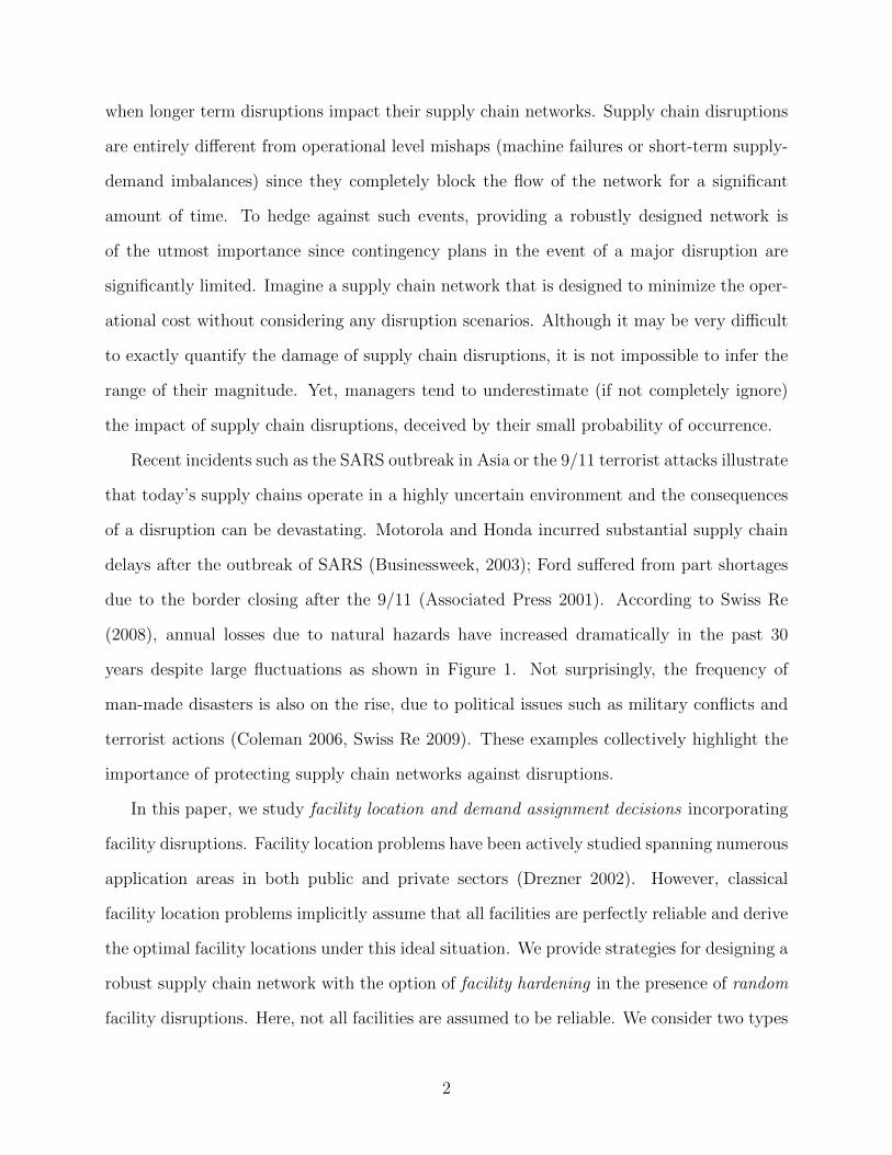
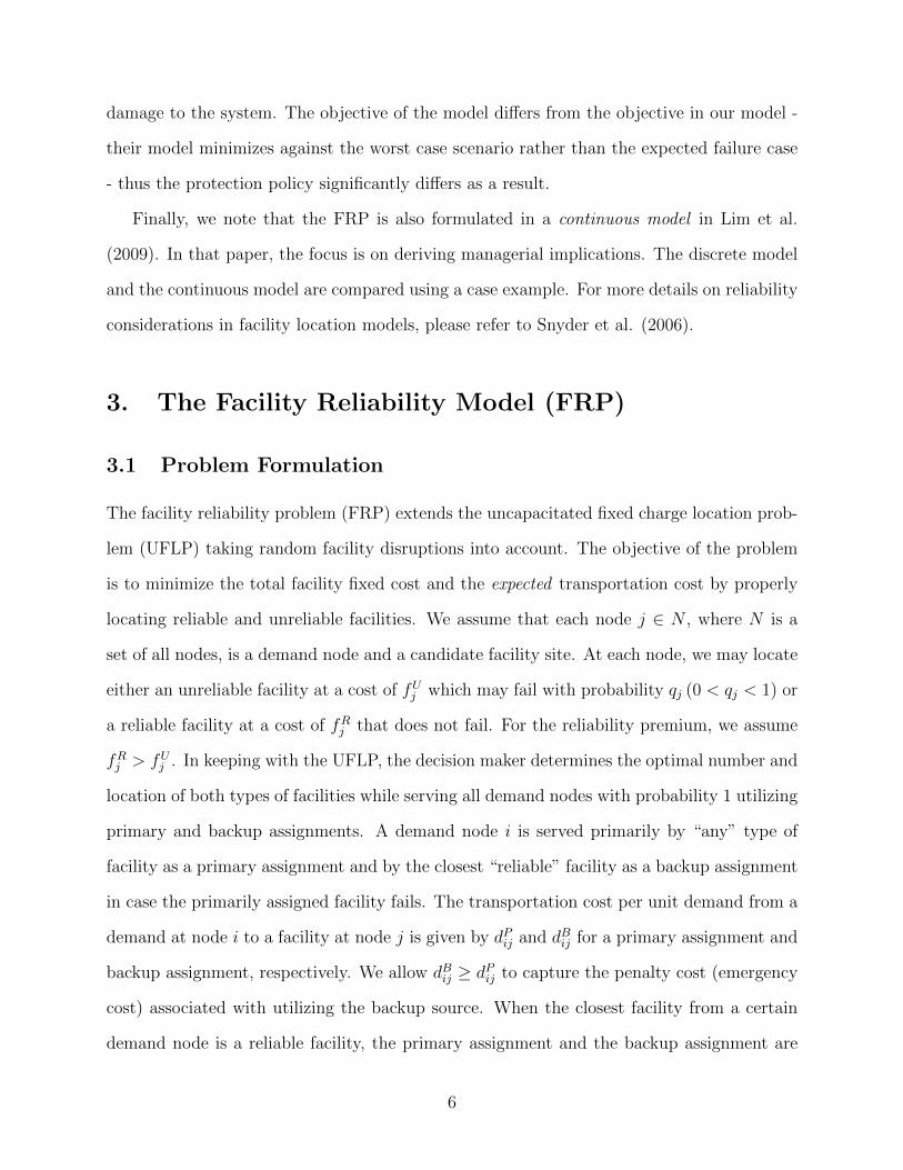
Modified Case Examples. We also numerically confirmed Theorems 1 and 2 by changing the

disruption probabilities. Figure 3(a) corresponds to the case in which q is large (Theorem 1) and

Figure 3(b) corresponds to the case in which q is small (Theorem 2). Here, we set qj = q = 0.2 and

20

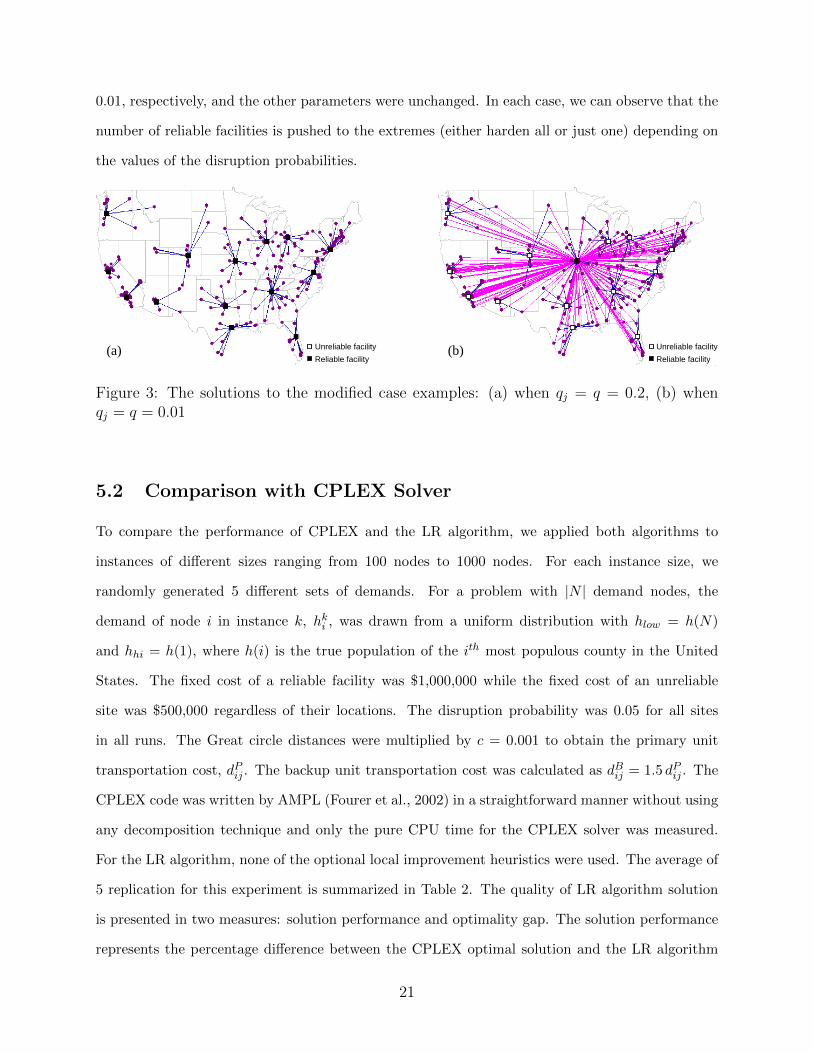
0.01, respectively, and the other parameters were unchanged. In each case, we can observe that the

number of reliable facilities is pushed to the extremes (either harden all or just one) depending on

the values of the disruption probabilities.

Unreliable facilityReliable facility

(a) Unreliable facilityReliable facility

(b)

Figure 3: The solutions to the modified case examples: (a) when qj = q = 0.2, (b) whenqj = q = 0.01

5.2 Comparison with CPLEX Solver

To compare the performance of CPLEX and the LR algorithm, we applied both algorithms to

instances of different sizes ranging from 100 nodes to 1000 nodes. For each instance size, we

randomly generated 5 different sets of demands. For a problem with ∣N ∣ demand nodes, the

demand of node i in instance k, ℎki , was drawn from a uniform distribution with ℎlow = ℎ(N)

and ℎℎi = ℎ(1), where ℎ(i) is the true population of the itℎ most populous county in the United

States. The fixed cost of a reliable facility was $1,000,000 while the fixed cost of an unreliable

site was $500,000 regardless of their locations. The disruption probability was 0.05 for all sites

in all runs. The Great circle distances were multiplied by c = 0.001 to obtain the primary unit

transportation cost, dPij . The backup unit transportation cost was calculated as dBij = 1.5 dPij . The

CPLEX code was written by AMPL (Fourer et al., 2002) in a straightforward manner without using

any decomposition technique and only the pure CPU time for the CPLEX solver was measured.

For the LR algorithm, none of the optional local improvement heuristics were used. The average of

5 replication for this experiment is summarized in Table 2. The quality of LR algorithm solution

is presented in two measures: solution performance and optimality gap. The solution performance

represents the percentage difference between the CPLEX optimal solution and the LR algorithm

21

solution. LR optimality gap represents the gap between the lower and upper bound of the LR

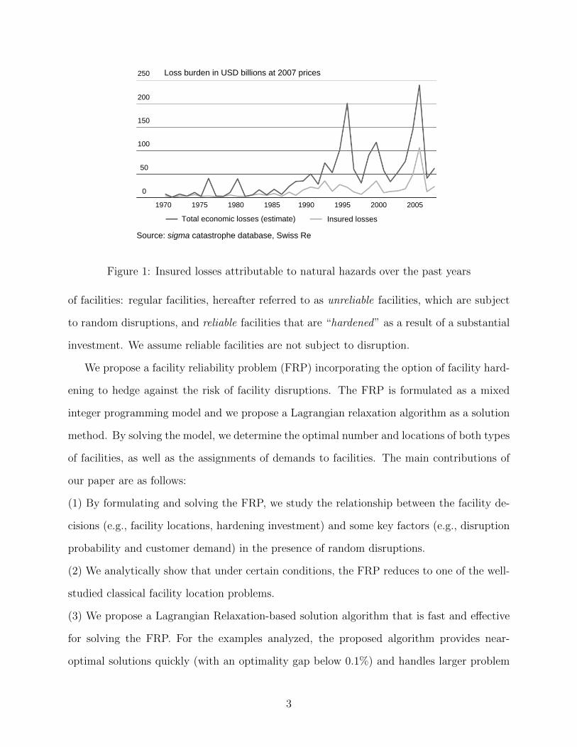
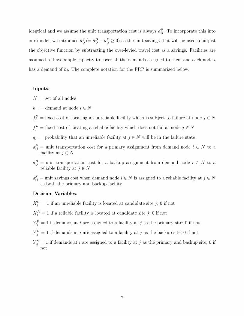
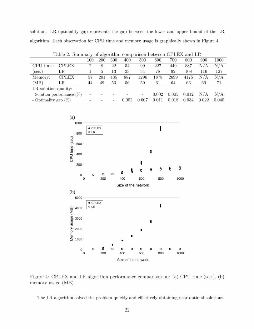
algorithm. Each observation for CPU time and memory usage is graphically shown in Figure 4.

Table 2: Summary of algorithm comparison between CPLEX and LR100 200 300 400 500 600 700 800 900 1000

CPU time: CPLEX 2 8 22 54 99 227 449 887 N/A N/A(sec.) LR 1 5 13 33 54 78 92 108 116 127

Memory: CPLEX 57 201 435 887 1296 1878 2699 4175 N/A N/A(MB) LR 44 49 53 56 59 61 64 66 69 71

LR solution quality:- Solution performance (%) - - - - - 0.002 0.005 0.012 N/A N/A- Optimality gap (%) - - - 0.002 0.007 0.011 0.018 0.034 0.022 0.040

0

200

400

600

800

1000

0 200 400 600 800 1000

Size of the network

CP

U ti

me

(sec

)

(a)

CPLEXLR

0 200 400 600 800 1000

1000

800

600

400

200

0

0

1000

2000

3000

4000

5000

0 200 400 600 800 1000Size of the network

Mem

ory

usag

e (M

B)

(b)

CPLEXLR

0 200 400 600 800 1000

5000

4000

3000

2000

1000

0

Figure 4: CPLEX and LR algorithm performance comparison on: (a) CPU time (sec.), (b)memory usage (MB)

The LR algorithm solved the problem quickly and effectively obtaining near-optimal solutions.

22

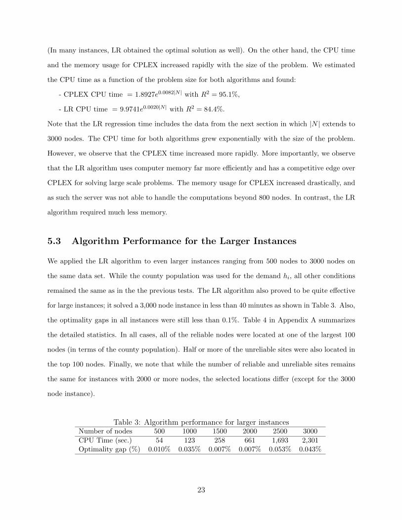
(In many instances, LR obtained the optimal solution as well). On the other hand, the CPU time

and the memory usage for CPLEX increased rapidly with the size of the problem. We estimated

the CPU time as a function of the problem size for both algorithms and found:

- CPLEX CPU time = 1.8927e0.0082∣N ∣ with R2 = 95.1%,

- LR CPU time = 9.9741e0.0020∣N ∣ with R2 = 84.4%.

Note that the LR regression time includes the data from the next section in which ∣N ∣ extends to

3000 nodes. The CPU time for both algorithms grew exponentially with the size of the problem.

However, we observe that the CPLEX time increased more rapidly. More importantly, we observe

that the LR algorithm uses computer memory far more efficiently and has a competitive edge over

CPLEX for solving large scale problems. The memory usage for CPLEX increased drastically, and

as such the server was not able to handle the computations beyond 800 nodes. In contrast, the LR

algorithm required much less memory.

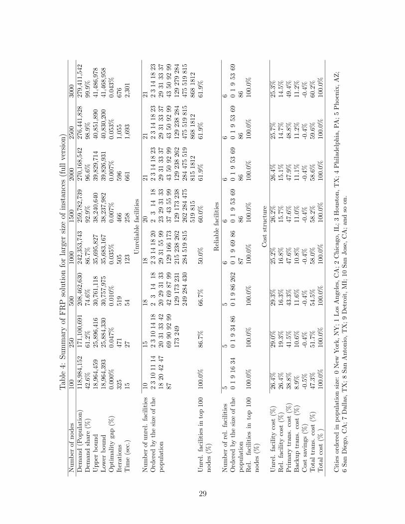
5.3 Algorithm Performance for the Larger Instances

We applied the LR algorithm to even larger instances ranging from 500 nodes to 3000 nodes on

the same data set. While the county population was used for the demand ℎi, all other conditions

remained the same as in the the previous tests. The LR algorithm also proved to be quite effective

for large instances; it solved a 3,000 node instance in less than 40 minutes as shown in Table 3. Also,

the optimality gaps in all instances were still less than 0.1%. Table 4 in Appendix A summarizes

the detailed statistics. In all cases, all of the reliable nodes were located at one of the largest 100

nodes (in terms of the county population). Half or more of the unreliable sites were also located in

the top 100 nodes. Finally, we note that while the number of reliable and unreliable sites remains

the same for instances with 2000 or more nodes, the selected locations differ (except for the 3000

node instance).

Table 3: Algorithm performance for larger instancesNumber of nodes 500 1000 1500 2000 2500 3000

CPU Time (sec.) 54 123 258 661 1,693 2,301Optimality gap (%) 0.010% 0.035% 0.007% 0.007% 0.053% 0.043%

23

6. Discussion and Conclusions

In this paper, we presented a facility reliability problem in the presence of random facility dis-

ruptions. We formulated the problem of determining how many hardened and non-hardened sites

to use as a mixed integer programming problem. We also outlined a solution algorithm based on

Lagrangian relaxation. Computational studies showed that the algorithm is fast (in terms of CPU

time) and efficient (in terms of memory usage) with a small optimality gap. We also showed that

this algorithm has a significant competitive edge over CPLEX particularly for solving large-scale

problems.

Our findings pose new questions and motivate additional future research. First, we have ignored

capacity issues in this study. While uncapacitated models provide valuable insights and guidelines

at the strategic level, exploring the effect of capacity issues would be interesting. We believe this

study provides a good starting point for research in this direction. Second, we do not account for

partial facility disruptions as well as partial hardening options (with less investment). While this

problem may be more realistic, some of the concepts in the problem have to be redefined such

as what backup assignments mean, how many backups are enough if no facility is totally reliable,

and so on. Lastly, it would be desirable to extend the model to cases in which the disruption

probabilities are not independent, but rather are correlated. This would enable us to construct a

network that is more robust against the worst case scenario.

Acknowledgments

The research was supported in part by the National Science Foundation (DMI-0457503) and the

Office of Naval Research (N00014-05-1-0190). This support is gratefully appreciated. Any opin-

ions, findings, and conclusions or recommendations expressed in this publication are those of the

author(s) and do not necessarily reflect the views of the National Science Foundation or the Office

of Naval Research.

24

References

[1] AP (Associated Press), Parts shortages cause Ford shutdown, Sep 14, 2001.

[2] R. Batta, J.M. Dolan, and N.N. Krishnamurthy, The maximal expected covering location problem

- revisited, Transport Sci 23(4) (1989), 277–287.

[3] R. Batta, and N.R. Mannur, Covering-location models for emergency situations that require mul-

tiple response units, Manage Sci 36(1) (1990), 16–23.

[4] O. Berman, D. Krass, and M. Menezes, Facility reliability issues in network p-Median problems:

Strategic centralization and co-location effects, Oper Res 55(2) (2007), 332–350.

[5] Businessweek, SARS: The Sequel? Oct 27, 2003.

[6] S. Chopra, G. Reinhardt, and U. Mohan, The importance of decoupling recurrent and disruption

risks in a supply chain, Nav Res Log 54(5) (2007), 544–555.

[7] R.L. Church, and M.P. Scaparra, Protecting critical assets: The r-interdiction median problem

with fortification, Geogr Anal 39(2) (2007), 129–146.

[8] L. Coleman, Frequency of man-made disasters in the 20th century, J Conting Crisis Manage 14(1)

(2006), 3–11.

[9] H. Crowder, “Computational improvements for subgradient optimization,” Symposia Mathematica

19, Academic Press, New York, 1976, pp. 357–371.

[10] T. Cui, Y. Ouyang, and Z.-J.M. Shen, Reliable facility location design under the risk of disruptions.

Working paper, Department of Industrial Engineering and Operations Research, University of

California at Berkeley, 2008.

[11] M.S. Daskin, A maximum expected covering location model: Formulation, properties and heuristic

solution, Transport Sci 17(1) (1983), 48–70.

[12] M.S. Daskin, Network and discrete location: Models, algorithms and applications, John Wiley and

Sons, Inc., New York, 1995.

[13] Z. Drezner, Heuristic solution methods for two location problems with unreliable facilities, J Oper

Res Soc 38(6) (1987), 509–514.

25

[14] Z. Drezner, and H.W. Hamacher, Facility location: Application and theory, Springer, Berlin, Ger-

many, 2002.

[15] M.L. Fisher, The Lagrangian relaxation method for solving integer programming problems, Manage

Sci 27(1) (1981), 1–18.

[16] M.L. Fisher, An applications oriented guide to Lagrangian relaxation, Interfaces 15(2) (1985), 10–

21.

[17] R. Fourer, D.M. Gay, and B.W. Kernighan, AMPL: A modeling language for mathematical pro-

gramming, Duxbury Press, California, 2002.

[18] K. Hogan, and C. ReVelle, Concepts and applications of backup coverage, Manage Sci 32(11)

(1986), 1434–1444.

[19] M. Lim, M.S. Daskin, A. Bassamboo, and S. Chopra, Facility location decisions in supply chain

networks with random disruption and imperfect information. Working paper, Department of

Industrial Engineering and Management Sciences, Northwestern University, 2009.

[20] H. Pirkul, The uncapacitated facility location problem with primary and secondary facility require-

ments, IIE Trans 21(4) (1989), 337–348.

[21] H. Pirkul, and D.A. Schilling, The siting of emergency service facilities with workload capacities

and backup service, Manage Sci 34(7) (1988), 896–908.

[22] C. ReVelle, and K. Hogan, The maximum availability location problem, Transport Sci 23(3) (1989),

192–200.

[23] M.P. Scaparra, and R.L. Church, A bilevel mixed integer program for critical infrastructure pro-

tection planning, Comput Oper Res 35(6) (2008), 1905–1923.

[24] L.V. Snyder, and M.S. Daskin, Reliability models for facility location: The expected failure cost

case, Transport Sci 39(3) (2005), 400–416.

[25] L.V. Snyder, and M.S. Daskin, Stochastic p-robust location problems, IIE Trans 38(11) (2006),

971–985.

[26] L.V. Snyder, P.M. Scaparra, M.S. Daskin, and R.L. Church, Planning for disruptions in supply

chain networks, TutORials in Operations Research, INFORMS, 2006.

26

[27] Swiss Re, Focus report: Disaster risk financing, 2008. Available online via

<http://www.preventionweb.net/files/3224 3224SwissRePubl08FRDisasterriskfinancing.pdf>.

[28] Swiss Re, Sigma report: Natural catastrophes and Man-made disasters, 2009. Available online via

<http://www.swissre.com/resources/dd6346004d4e9669ac76eecedd316cf3-sigma2 2009 e.pdf>.

[29] B. Tomlin, On the value of mitigation and contingency strategies for managing supply chain dis-

ruption risks, Manage Sci 52(5) (2006), 639–657.

[30] R.L. Zhan, Z.-J.M. Shen, and M.S. Daskin. System reliability with location-specific failure proba-

bilities. Working paper, Department of Industrial Engineering and Operations Research, Uni-

versity of California at Berkeley, 2007.

27

Appendix

Appendix A: Summary of FRP solution for larger instances

28

Tab

le4:

Sum

mar

yof

FR

Pso

luti

onfo

rla

rger

size

ofin

stan

ces

(full

vers

ion)

Nu

mb

erof

nod

es10

025

0500

1000

1500

2000

2500

3000

Dem

and

(Pop

ula

tion

)11

8,98

4,15

217

1,1

00,6

91

208,4

62,6

30

242,3

53,7

43

259,7

82,7

39

270,1

68,5

42

276,4

41,8

28

279,4

11,5

42

Dem

and

shar

e(%

)42

.6%

61.2

%74.6

%86.7

%92.9

%96.6

%98.9

%99.9

%U

pp

erb

oun

d18

,964

,459

25,8

96,4

16

30,7

61,1

18

35,6

95,8

27

38,2

40,6

40

39,8

29,7

14

40,8

51,8

90

41,4

86,9

78

Low

erb

oun

d18

,964

,393

25,8

84,3

30

30,7

57,9

75

35,6

83,1

67

38,2

37,9

82

39,8

26,9

31

40,8

30,2

00

41,4

68,9

58

Op

tim

alit

yga

p(%

)0.

000%

0.04

7%

0.0

10%

0.0

35%

0.0

07%

0.0

07%

0.0

53%

0.0

43%

Iter

atio

ns

325

471

519

505

466

596

1,0

55

676

Tim

e(s

ec.)

1527

54

123

258

661

1,6

93

2,3

01

Un

reli

ab

lefa

cili

ties

Nu

mb

erof

un

rel.

faci

liti

es10

1518

18

20

21

21

21

Ord

ered

by

the

size

ofth

ep

opu

lati

on2

310

1114

1820

4247

87

23

10

14

18

2031

33

42

6990

92

99

173

249

23

14

18

20

29

31

33

42

69

87

99

129

173

231

249

284

430

23

14

18

20

29

31

55

99

129

166

173

215

238

262

284

519

815

23

14

18

23

29

31

33

37

43

55

99

129

173

238

262

284

475

519

815

23

14

18

23

29

31

33

37

43

50

92

99

129

238

262

284

475

519

815

1812

23

14

18

23

29

31

33

37

43

50

92

99

129

238

284

475

519

815

868

1812

23

14

18

23

29

31

33

37

43

50

92

99

129

279

284

475

519

815

868

1812

Un

rel.

faci

liti

esin

top

100

nod

es(%

)10

0.0%

86.7

%66.7

%50.0

%60.0

%61.9

%61.9

%61.9

%

Rel

iab

lefa

cili

ties

Nu

mb

erof

rel.

faci

liti

es5

55

66

66

6O

rder

edby

the

size

ofth

ep

opu

lati

on0

19

1634

01

934

86

01

986

262

01

969

86

87

01

953

69

86

01

953

69

86

01

953

69

86

01

953

69

86

Rel

.fa

cili

ties

into

p10

0n

od

es(%

)10

0.0%

100.

0%

100.0

%100.0

%100.0

%100.0

%100.0

%100.0

%

Cost

stru

ctu

re

Un

rel.

faci

lity

cost

(%)

26.4

%29

.0%

29.3

%25.2

%26.2

%26.4

%25.7

%25.3

%R

el.

faci

lity

cost

(%)

26.4

%19

.3%

16.3

%16.8

%15.7

%15.1

%14.7

%14.5

%P

rim

ary

tran

s.co

st(%

)38

.8%

41.5

%43.3

%47.6

%47.6

%47.9

%48.8

%49.4

%B

acku

ptr

ans.

cost

(%)

8.9%

10.6

%11.6

%10.8

%11.0

%11.1

%11.2

%11.2

%C

ost

savin

gs(%

)-0

.5%

-0.4

%-0

.4%

-0.4

%-0

.4%

-0.4

%-0

.4%

-0.4

%T

otal

tran

s.co

st(%

)47

.3%

51.7

%54.5

%58.0

%58.2

%58.6

%59.6

%60.2

%T

otal

cost

(%)

100.

0%10

0.0

%100.0

%100.0

%100.0

%100.0

%100.0

%100.0

%

Cit

ies

ord

ered

inp

opu

lati

onsi

ze:

0N

ewY

ork,

NY

;1

Los

An

gel

es,

CA

;2

Ch

icago,

IL;

3H

ou

ston

,T

X;

4P

hil

ad

elp

hia

,P

A;

5P

hoen

ix,

AZ

;6

San

Die

go,

CA

;7

Dal

las,

TX

;8

San

Anto

nio

,T

X;

9D

etro

it,

MI;

10

San

Jose

,C

A;

an

dso

on.

29