Embed Size (px)
Citation preview
A Feasibility Study of Solar PV in Reducing
Peak Electrical Demand and Consumption
Costs in Commercial Buildings in
Melbourne
Joel Seagren
Dissertation for Master of Science in Renewable Energy
School of Engineering and Energy
Murdoch University
2013
_________________________________________________________________________ i
Declaration
This dissertation is an authentic account of original research conducted by me which
has not been submitted towards another degree.
Joel Seagren
March 2013
_________________________________________________________________________ ii
Abstract
A significant part of the electricity cost of commercial buildings in Melbourne is due to high
peak demand that usually occurs on hot summer afternoons. Installation of solar PV on
commercial facilities to reduce this cost is not as wide spread as it is in the residential
section, despite sharp increases in electricity prices and falling solar PV system costs.
Existing literature has identified peak demand on transformers servicing commercial
buildings in Melbourne as having a high coincidence in timing with high PV system output.
This thesis investigates the feasibility of using solar PV to reduce electricity consumption
and peak electricity demand in Melbourne commercial buildings to reduce electricity cost.
It also investigates the technical issues involved, and whether such a system would be
considered financially feasible by businesses in today’s market.
A case study was conducted on a commercial facility (a Coles supermarket) in Melbourne
to determine how well its peak demand profile matches PV output from a local array, the
reliability of such a system in offsetting peak demand, and the potential savings based on
the tariff in place.
The results show that only a maximum of 30% of PV system rated power output can be
reliably counted upon to offset peak demand in summer. The timing of high PV output,
whilst better than in residential applications, may still not coincide exactly with peak
demand periods when using a north facing array to maximise annual energy output. In the
case study and for other buildings with early afternoon demand peaks (typical of cooling
related demand), an array rotated approximately 50 degrees to the west of True North,
would provide an increase in demand offset, and a net increase in financial benefit. This
maximum PV penetration could reduce a commercial building’s annual grid electricity cost
by $144 per kW installed depending on the tariff structure in place.
_________________________________________________________________________ iii
PV synched demand management is an alternative that could improve the effectiveness
of such a system, by temporarily reducing building demand during periods of low PV
output, so that peak demand event is avoided.
In conclusion, commercial buildings with summer peak demand that is substantially higher
than winter, are better suited to PV offset due to tariff structures, and solar resource
availability. These typically include buildings that have high cooling demands, such as
office buildings, supermarkets, universities, and hospitals.

_________________________________________________________________________ iv
Acknowledgements
I would like to acknowledge the help of Dr Jonathan Whale and Dr Samuel Gyamfi for
their support in guiding and shaping this work. In addition a big thank you goes to Paul
Lang of Coles who generously supplied consumption and demand data, and answered
questions throughout this piece of work, and the Melbourne City Council who kindly
provided Solar PV data from their Queen Victoria Market site.
_________________________________________________________________________ v
Table of Contents
Declaration ............................................................................................................................... i
Abstract ................................................................................................................................... ii
Table of Contents .................................................................................................................... v
List of Figures ....................................................................................................................... vii
Definitions ............................................................................................................................ viii
Chapter 1 – Introduction ............................................................................................................. 1
1.1 Motivation for the research ............................................................................................... 1
1.2 Research Question ............................................................................................................ 3
1.3 Scope ................................................................................................................................. 4
Chapter 2 – Existing Literature ................................................................................................... 5
2.1 Peak Demand .................................................................................................................... 5
Chapter - 3 Methodology .......................................................................................................... 13
3.1 Research Methodology. .................................................................................................. 13
Chapter 4 – Case Study Background ....................................................................................... 15
4.1 Building Details ............................................................................................................... 15
4.2 PV System Details ........................................................................................................... 16
Chapter 5 – Technical Feasibility ............................................................................................. 18
5.1 Electricity Consumption and Demand ............................................................................ 18
5.2 Tariff Structure ................................................................................................................ 21
5.3 Solar PV data ................................................................................................................... 23
5.4 Coincidence between PV output and Demand ............................................................... 24
5.5 Sensitivity Analysis ......................................................................................................... 27
5.5.1 Sensitivity Analysis of Daily Demand Profile and PV Array Rotation ........................ 28
_________________________________________________________________________ vi
5.6 Alternative solutions ....................................................................................................... 29
Chapter 6 – Financial Feasibility .............................................................................................. 32
6.1 Ideal theoretical maximum potential savings ................................................................ 32
6.2 Practical potential savings.............................................................................................. 33
6.3 Available Government Rebates ...................................................................................... 33
6.4 PV System Costs ............................................................................................................. 34
6.5 Financial Feasibility Indicators ....................................................................................... 35
Chapter 7 – Discussion of results ............................................................................................ 38
7.1 Demand Observations ................................................................................................. 38
7.2 PV output observations .............................................................................................. 38
7.3 Sensitivity of results to varying demand profiles and PV array orientations ........... 39
7.4 Enhancements to PV system ...................................................................................... 40
7.5 Technical Feasibility Result ........................................................................................ 42
7.6 Financial Feasibility Result ......................................................................................... 42
7.7 Limitations of Results ................................................................................................. 44
Chapter 8 – Conclusion ............................................................................................................ 45
References ................................................................................................................................ 47
Appendix A ............................................................................................................................ 53
Appendix B ............................................................................................................................ 54
Appendix C ............................................................................................................................ 55
Appendix D ............................................................................................................................ 56
Appendix E ............................................................................................................................ 57
_________________________________________________________________________ vii
List of Figures
Figure 1. Summer Electricity Demand Makeup for NSW
Figure 2. Comparative Proportion of Commercial Building Consumption and
Demand Impact by Application
Figure 3. The Forecast Fall in PV Module Costs
Figure 4. Coincidence of transformer commercial load and PV
Figure 5. Coincidence of NEM Load and PV output
Figure 6. PV output from 30 localised sites
Figure 7. Aerial view of Sommerville Coles Store
Figure 8. 30 Minute peak electrical demand for case study building
Figure 9. Peak demand profiles curves for Feb 2012
Figure 10. Demand duration curve for Feb 2012
Figure 11. Retailer, Distributor, and Misc. tariffs
Figure 12. 15 min PV output Energy
Figure 13. Effect of PV output on Peak demand curve during peak demand.
Figure 14. Effect of PV output on Peak demand curve during peak demand.
_________________________________________________________________________ viii
Definitions
Consumption Electricity used (measured in kWh)
Demand Average value of electric load over a period of time (known as the
demand interval)
Demand Management The planning, implementation and monitoring of those utility
activities designed to influence customer use of electricity in ways
that will produce desired change in the utilities load shape. i.e.
changes in the time pattern and magnitude of a utility’s load
(Gellings, 1981)
Peak Demand The maximum demand that has occurred over a specified period of
time.
PV System Solar Photovoltaic System
Tariff Schedule of charges for supply, consumption and demand of
electricity levied by electricity retailers and distributors.
_________________________________________________________________________ 1
Chapter 1 – Introduction
1.1 Motivation for the research
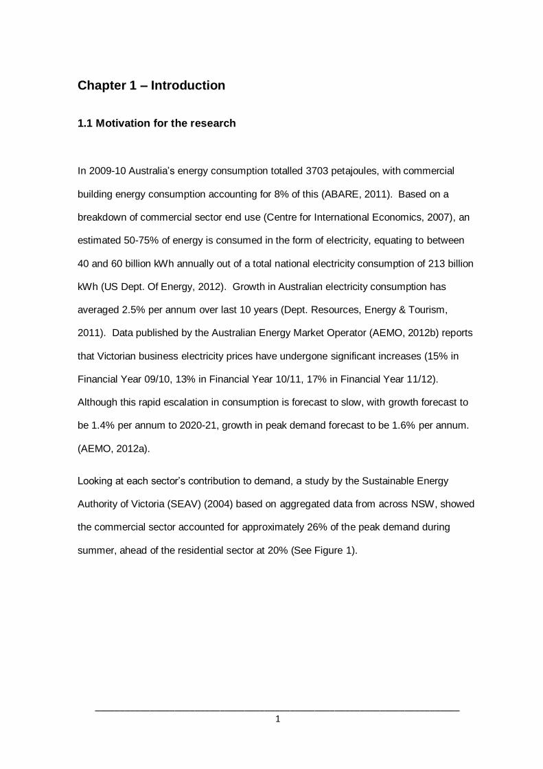
In 2009-10 Australia’s energy consumption totalled 3703 petajoules, with commercial
building energy consumption accounting for 8% of this (ABARE, 2011). Based on a
breakdown of commercial sector end use (Centre for International Economics, 2007), an
estimated 50-75% of energy is consumed in the form of electricity, equating to between
40 and 60 billion kWh annually out of a total national electricity consumption of 213 billion
kWh (US Dept. Of Energy, 2012). Growth in Australian electricity consumption has
averaged 2.5% per annum over last 10 years (Dept. Resources, Energy & Tourism,
2011). Data published by the Australian Energy Market Operator (AEMO, 2012b) reports
that Victorian business electricity prices have undergone significant increases (15% in
Financial Year 09/10, 13% in Financial Year 10/11, 17% in Financial Year 11/12).
Although this rapid escalation in consumption is forecast to slow, with growth forecast to
be 1.4% per annum to 2020-21, growth in peak demand forecast to be 1.6% per annum.
(AEMO, 2012a).
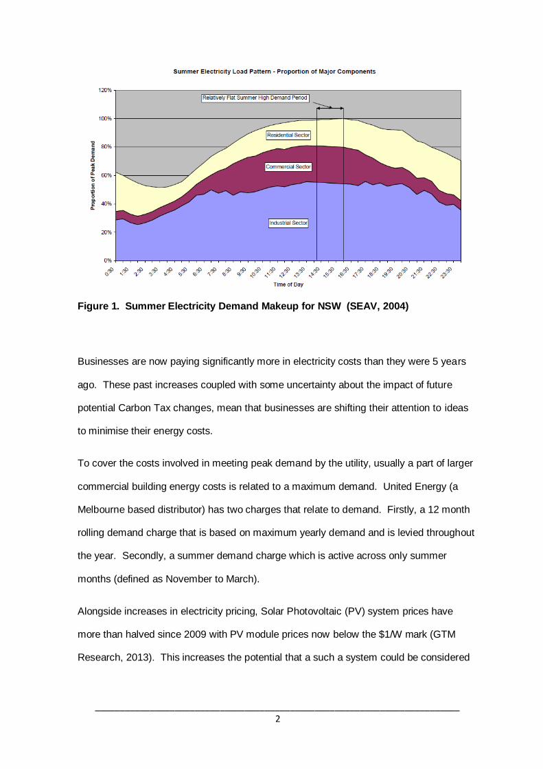
Looking at each sector’s contribution to demand, a study by the Sustainable Energy
Authority of Victoria (SEAV) (2004) based on aggregated data from across NSW, showed
the commercial sector accounted for approximately 26% of the peak demand during
summer, ahead of the residential sector at 20% (See Figure 1).
_________________________________________________________________________ 2
Figure 1. Summer Electricity Demand Makeup for NSW (SEAV, 2004)
Businesses are now paying significantly more in electricity costs than they were 5 years
ago. These past increases coupled with some uncertainty about the impact of future
potential Carbon Tax changes, mean that businesses are shifting their attention to ideas
to minimise their energy costs.
To cover the costs involved in meeting peak demand by the utility, usually a part of larger
commercial building energy costs is related to a maximum demand. United Energy (a
Melbourne based distributor) has two charges that relate to demand. Firstly, a 12 month
rolling demand charge that is based on maximum yearly demand and is levied throughout
the year. Secondly, a summer demand charge which is active across only summer
months (defined as November to March).
Alongside increases in electricity pricing, Solar Photovoltaic (PV) system prices have
more than halved since 2009 with PV module prices now below the $1/W mark (GTM
Research, 2013). This increases the potential that a such a system could be considered
_________________________________________________________________________ 3
financially feasible by commercial building tenants in reducing both electricity
consumption and peak demand costs.
This dissertation examines the potential of PV systems to offset peak demand events in
commercial buildings in Melbourne, and consequently reduce the costs associated with
both peak demand and consumption of electricity. A Coles Supermarket located near
Melbourne is used as a case study building to investigate the feasibility of such a system.
1.2 Research Question
The research question around which this thesis is based can be formulated as follows:
“Is Solar PV likely to be considered feasible in reducing peak electrical demand and
consumption costs in commercial buildings in Melbourne?”
This thesis aims to answer this research question using a set of specific objectives.
These objectives are:
To gauge the level of coincidence in timing of high PV system output and peak
electrical demand for the case study building, and therefore for other similar
commercial buildings in Melbourne.
To assess the reliability of a typical PV system output in Melbourne and assess to
what degree it is capable of reliably offsetting peak demand events.
To examine whether solar PV could currently be considered technically and
financially feasible in reducing electrical peak demand charges for the case study
building, and for other similar commercial buildings.
To investigate whether there are any enhancements that could improve the ability
of PV systems to offset peak demand events.
_________________________________________________________________________ 4
To identify some characteristics of commercial building peak demands that may
increase their suitability for PV system offset.
1.3 Scope
This study looks at the electrical demand and consumption characteristics of a case study
building, and assesses the feasibility of locally generated solar PV electricity in reducing
demand and consumption charges. It considers the correlation in timing between peak
demand events and peak PV output in Melbourne during summer periods, assesses the
reliability of PV output, and consequently the ability to offset a peak demand event. It then
offers some ideas to enhance a PV system output to improve the reliability.
The study focuses on commercial buildings as existing literature suggests higher
coincidence of high PV output and peak demand. No consideration of issues affecting
residential applications is given.
PV system data and tariff information used in the case study is from Melbourne and other
tariff structures and PV output characteristic that may exist in other states are not
considered.
Apart from some brief observations, it does not breakdown demand or consumption in
detail (e.g. cooling, lighting etc.). The accuracy of consumption and demand data
provided by Coles, and PV system data by the Melbourne City Council, has not been
verified, although data with obvious errors or omissions has not been used.
_________________________________________________________________________ 5
Chapter 2 – Existing Literature
2.1 Peak Demand
To understand a little more about peak demand it is first necessary to define what is
meant by this term. Demand can be defined as the average value of electric load over a
specified period of time, and consequently peak demand is the maximum demand that
occurs over a specified period. Why is peak demand of interest to both utility companies
and consumers, in particular commercial consumers? To answer this question it is
necessary to review the causes and costs associated with meeting peak electricity
demands on utilities’ networks.
Peak demand occurs as a result of coincidence in demand of many end-use appliances.
A sample of Sydney commercial office buildings analysed showed that an average of 15%
of demand capacity is required for just 1% of the time (Steinfeld et al.,2011). An earlier
study found that 10% of Energy Australia’s network capacity in New South Wales is used
for <1% of the time (Dunstan et al, 2008). This requires utilities to provide and maintain
generating equipment of up to 10-15% of total capacity that may only be used for 1% of
the year. Because of the low use and urgency with which it can sometimes be required,
this generating equipment typically needs to be of a type that can be brought online
quickly. As a result peak power plants usually run on natural gas or diesel, which have
high operating costs compared to base load supply equipment, and emit greenhouse
gases.
Increasing demand for electricity during periods of peak consumption not only requires
higher unit cost generation equipment to be brought online, but also significant investment
in network infrastructure. In the Sydney Metro area the network augmentation to meet
forecast peak demand for 2012/13 was in estimated to cost in excess of $200 million
_________________________________________________________________________ 6
(Energy Australia, 2007). These increased costs to electricity generators required to
service periods of peak demand (Australian Energy Regulator, 2009) mean that it is not
surprising that at least some of this cost is passed onto consumers. United Energy
passes on peak demand charges to all larger consumers (> 400 MWh) (United Energy,
2011)) with some smaller consumers given the choice of having demand charges in
exchange for lower consumption charges.
An alternative to the supply-side investments is to focus on managing the peak demand.
Demand-side management is the planning, implementation and monitoring of those utility
activities designed to influence customer use of electricity in ways that will produce
desired change in the utilities load shape, i.e. changes in the time pattern and magnitude
of a utility’s load (Gellings, 1981). Methods that can be used to manage peak demand
include the use of onsite generation and storage of electricity for use during peak times
(Shugar,1990) (Stadler, 2007) power system optimization algorithms that can prevent
blackout during peak time (Hope, 2007), energy efficiency improvements (York, 2005),
and demand response (Gyamfi,2012).
It has been estimated that reducing peak demand for the Sydney Metro area by around
75MVA by 2012/13, and 100MVA per year each year after would indefinitely defer the
requirement for network augmentation to meet peak demand (Energy Australia, 2007)
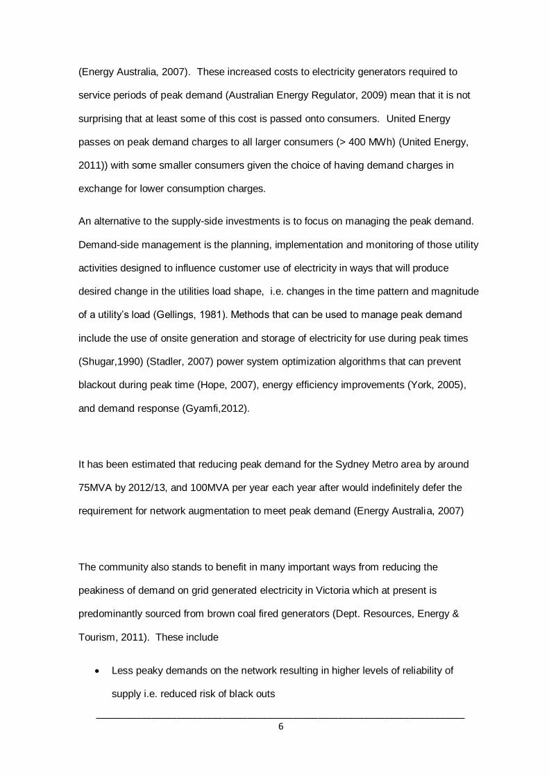
The community also stands to benefit in many important ways from reducing the
peakiness of demand on grid generated electricity in Victoria which at present is
predominantly sourced from brown coal fired generators (Dept. Resources, Energy &
Tourism, 2011). These include
Less peaky demands on the network resulting in higher levels of reliability of
supply i.e. reduced risk of black outs
_________________________________________________________________________ 7
Less investment in infrastructure to service peak demands is required, the cost of
which ultimately flows to most consumers either directly via utility charges or
indirectly in the form or taxes etc.
Potential for reduced greenhouse gas emissions associated with electricity
generation as peaking generation equipment can be less energy efficient
(compared to baseload)
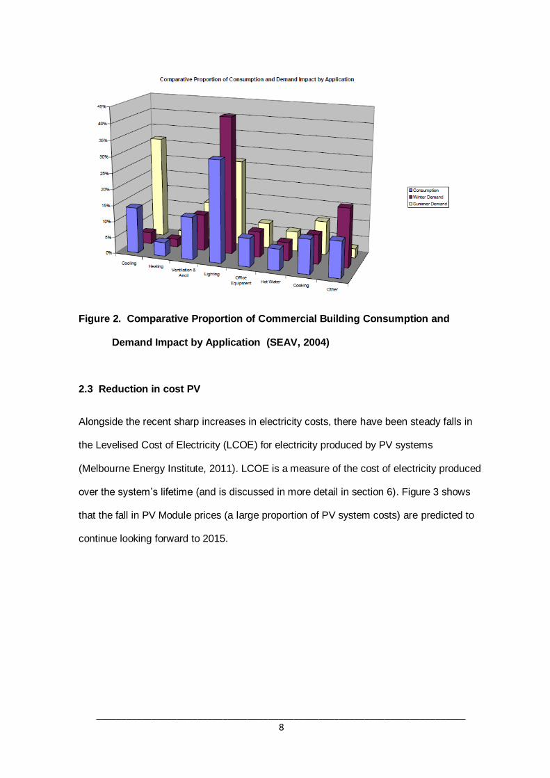
Whilst the peak demand was greatest during the summer period, it was only 10% greater
than for the winter period. The total was then broken into commercial sector applications,
to show which applications contributed the most to summer or winter demand relative to
their annual use. This was done by dividing the peak demand in Megawatts (MW) (for
summer & winter) by the annual electricity consumption in PetaJoules (PJ). Figure 2
shows that cooling during the summer period is (as expected) the largest contributor to
peak demand relative to average annual levels, whilst other applications (such as lighting,
ventilation, and office equipment) contributed very little to peak demand beyond their
average annual levels.
_________________________________________________________________________ 8
Figure 2. Comparative Proportion of Commercial Building Consumption and
Demand Impact by Application (SEAV, 2004)
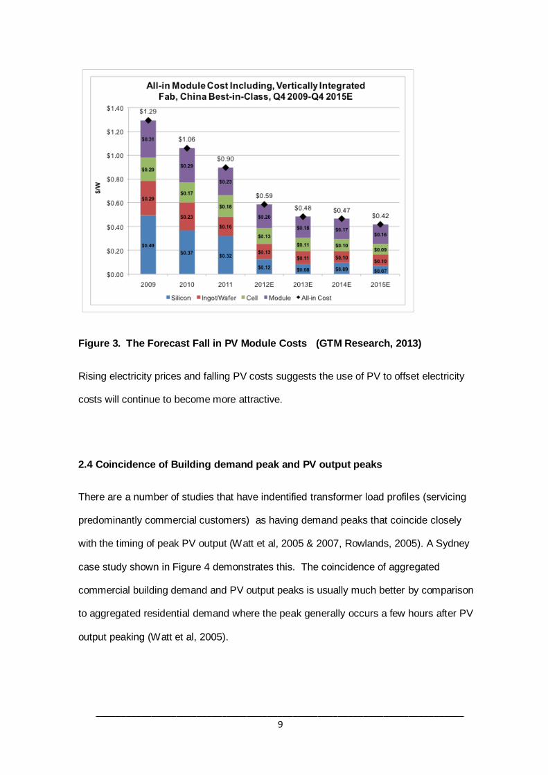
2.3 Reduction in cost PV
Alongside the recent sharp increases in electricity costs, there have been steady falls in
the Levelised Cost of Electricity (LCOE) for electricity produced by PV systems
(Melbourne Energy Institute, 2011). LCOE is a measure of the cost of electricity produced
over the system’s lifetime (and is discussed in more detail in section 6). Figure 3 shows
that the fall in PV Module prices (a large proportion of PV system costs) are predicted to
continue looking forward to 2015.
_________________________________________________________________________ 9
Figure 3. The Forecast Fall in PV Module Costs (GTM Research, 2013)
Rising electricity prices and falling PV costs suggests the use of PV to offset electricity
costs will continue to become more attractive.
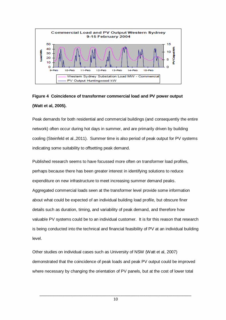
2.4 Coincidence of Building demand peak and PV output peaks
There are a number of studies that have indentified transformer load profiles (servicing
predominantly commercial customers) as having demand peaks that coincide closely
with the timing of peak PV output (Watt et al, 2005 & 2007, Rowlands, 2005). A Sydney
case study shown in Figure 4 demonstrates this. The coincidence of aggregated
commercial building demand and PV output peaks is usually much better by comparison
to aggregated residential demand where the peak generally occurs a few hours after PV
output peaking (Watt et al, 2005).
_________________________________________________________________________ 10
Figure 4 Coincidence of transformer commercial load and PV power output
(Watt et al, 2005).
Peak demands for both residential and commercial buildings (and consequently the entire
network) often occur during hot days in summer, and are primarily driven by building
cooling (Steinfeld et al.,2011). Summer time is also period of peak output for PV systems
indicating some suitability to offsetting peak demand.
Published research seems to have focussed more often on transformer load profiles,
perhaps because there has been greater interest in identifying solutions to reduce
expenditure on new infrastructure to meet increasing summer demand peaks.
Aggregated commercial loads seen at the transformer level provide some information
about what could be expected of an individual building load profile, but obscure finer
details such as duration, timing, and variability of peak demand, and therefore how
valuable PV systems could be to an individual customer. It is for this reason that research
is being conducted into the technical and financial feasibility of PV at an individual building
level.
Other studies on individual cases such as University of NSW (Watt et al, 2007)
demonstrated that the coincidence of peak loads and peak PV output could be improved
where necessary by changing the orientation of PV panels, but at the cost of lower total
_________________________________________________________________________ 11
output over the year. In these cases tariff structure and pricing would determine whether
trimming of peak demand is more valuable than maximising total energy production.
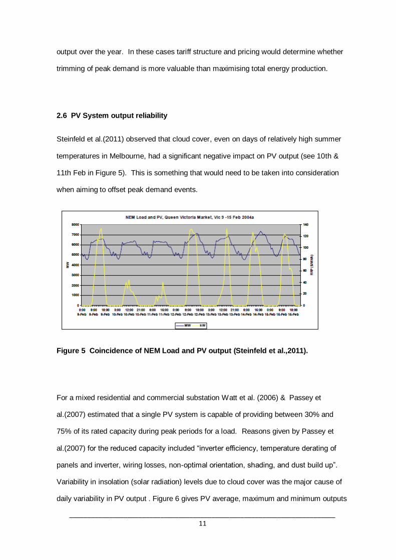
2.6 PV System output reliability
Steinfeld et al.(2011) observed that cloud cover, even on days of relatively high summer
temperatures in Melbourne, had a significant negative impact on PV output (see 10th &
11th Feb in Figure 5). This is something that would need to be taken into consideration
when aiming to offset peak demand events.
Figure 5 Coincidence of NEM Load and PV output (Steinfeld et al.,2011).
For a mixed residential and commercial substation Watt et al. (2006) & Passey et
al.(2007) estimated that a single PV system is capable of providing between 30% and
75% of its rated capacity during peak periods for a load. Reasons given by Passey et
al.(2007) for the reduced capacity included “inverter efficiency, temperature derating of
panels and inverter, wiring losses, non-optimal orientation, shading, and dust build up”.
Variability in insolation (solar radiation) levels due to cloud cover was the major cause of
daily variability in PV output . Figure 6 gives PV average, maximum and minimum outputs
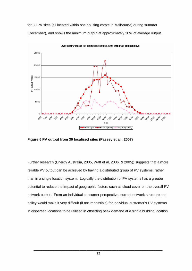
_________________________________________________________________________ 12
for 30 PV sites (all located within one housing estate in Melbourne) during summer
(December), and shows the minimum output at approximately 30% of average output.
Figure 6 PV output from 30 localised sites (Passey et al., 2007)
Further research (Energy Australia, 2005, Watt et al, 2006, & 2005)) suggests that a more
reliable PV output can be achieved by having a distributed group of PV systems, rather
than in a single location system. Logically the distribution of PV systems has a greater
potential to reduce the impact of geographic factors such as cloud cover on the overall PV
network output. From an individual consumer perspective, current network structure and
policy would make it very difficult (if not impossible) for individual customer’s PV systems
in dispersed locations to be utilised in offsetting peak demand at a single building location.
_________________________________________________________________________ 13
Chapter - 3 Methodology
3.1 Research Methodology.
The aim of the literature review was to understand where the best opportunities sat in
terms of utilizing a PV system for peak demand offset, and where the potential issues
may lie. This chapter focuses on the methodology that is applied to the case study, and to
the application of findings to other similar buildings.
The basic methodology was as follows.
Electricity demand and consumption data sourced for a case study commercial
building (Coles Supermarket located near Melbourne). This was provided by
Coles, who had sourced it from Origin Energy’s data logging facilities.
Solar PV system data sourced from Melbourne City Council’s (MCC) solar array
located on the roof of the Queen Victoria Market in Melbourne. This was recorded
by MCC data logging equipment.
30 minute demand data was then overlayed with PV output to assess the
coincidence in timing of peak demand events and high PV output.
Reliability of PV output was assessed using PV array data to determine the
likelihood of eliminating a peak demand event.
Consideration was given to other technical issues to determine whether a PV
system would be technically feasible in offsetting peak demand events
PV system costs evaluated
The potential avoided cost resulting from reduced peak demand and consumption
charges as a result of using a PV system was determined
Payback period calculated and compared to Coles investment criteria to determine
financial feasibility. LCOE calculated to provide an alternative measure.
_________________________________________________________________________ 14
Investigated technical alternatives that may enhance to capability of PV power to
offset peak demand events
Identified characteristics of the peak demand profile that improve the chance of
feasibility in other commercial buildings.
_________________________________________________________________________ 15
Chapter 4 – Case Study Background
4.1 Building Details
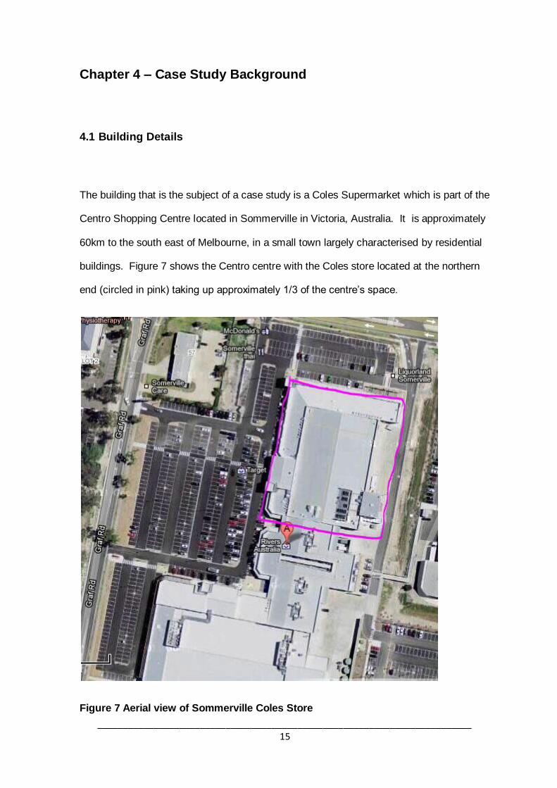
The building that is the subject of a case study is a Coles Supermarket which is part of the
Centro Shopping Centre located in Sommerville in Victoria, Australia. It is approximately
60km to the south east of Melbourne, in a small town largely characterised by residential
buildings. Figure 7 shows the Centro centre with the Coles store located at the northern
end (circled in pink) taking up approximately 1/3 of the centre’s space.
Figure 7 Aerial view of Sommerville Coles Store
_________________________________________________________________________ 16
The floor space occupied by the supermarket is in the order of 4000 m2, and its summer
time electrical demand arises from
space cooling
produce cooling (refrigeration and freezing)
ventilation
lighting
office and register equipment
food preparation equipment
Misc. equipment
This building was selected because of its suitability for a PV system on the roof, the
quantity and quality of electricity consumption data, and an interest by Coles in exploring
ways to reduce electricity costs and CO2 emissions.
In Australia supermarkets consume more than 7,000 GJ of electricity each year costing
around $200 million, and produce nearly three million tonnes of greenhouse gases.
Refrigeration accounts for the largest proportion of annual energy use at 55 per cent,
while air conditioning and lighting each account for 20 per cent. (Dept. of Industry,
Tourism, and Resources, 2004)
4.2 PV System Details
The PV system that has been selected to represent the potential of an average
Melbourne system is a large 200 kW array located on the roof of the Queen Victoria
market in inner Melbourne. It was selected again because of the quantity and quality of
data available, its good northerly orientation, and for being in relatively close proximity to
_________________________________________________________________________ 17
case study building. It is also in very close proximity to the large quantity of Melbourne
CBD buildings making it very representative of a system that could be applied to these
buildings. PV data is logged onsite and is kept by the Melbourne City Council.
Whilst not all buildings will have capacity to installing a 200 kW system, systems can be
easily scaled to appropriate size, and receive equally scaled benefits.
_________________________________________________________________________ 18
Chapter 5 – Technical Feasibility
5.1 Electricity Consumption and Demand
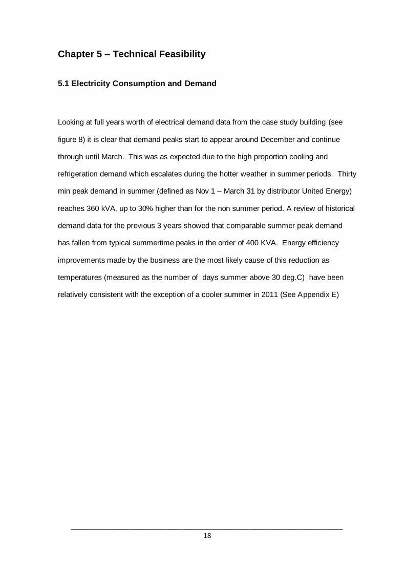
Looking at full years worth of electrical demand data from the case study building (see
figure 8) it is clear that demand peaks start to appear around December and continue
through until March. This was as expected due to the high proportion cooling and
refrigeration demand which escalates during the hotter weather in summer periods. Thirty
min peak demand in summer (defined as Nov 1 – March 31 by distributor United Energy)
reaches 360 kVA, up to 30% higher than for the non summer period. A review of historical
demand data for the previous 3 years showed that comparable summer peak demand
has fallen from typical summertime peaks in the order of 400 KVA. Energy efficiency
improvements made by the business are the most likely cause of this reduction as
temperatures (measured as the number of days summer above 30 deg.C) have been
relatively consistent with the exception of a cooler summer in 2011 (See Appendix E)
_________________________________________________________________________ 19
Figure 8. 30 Minute peak electrical demand for case study building
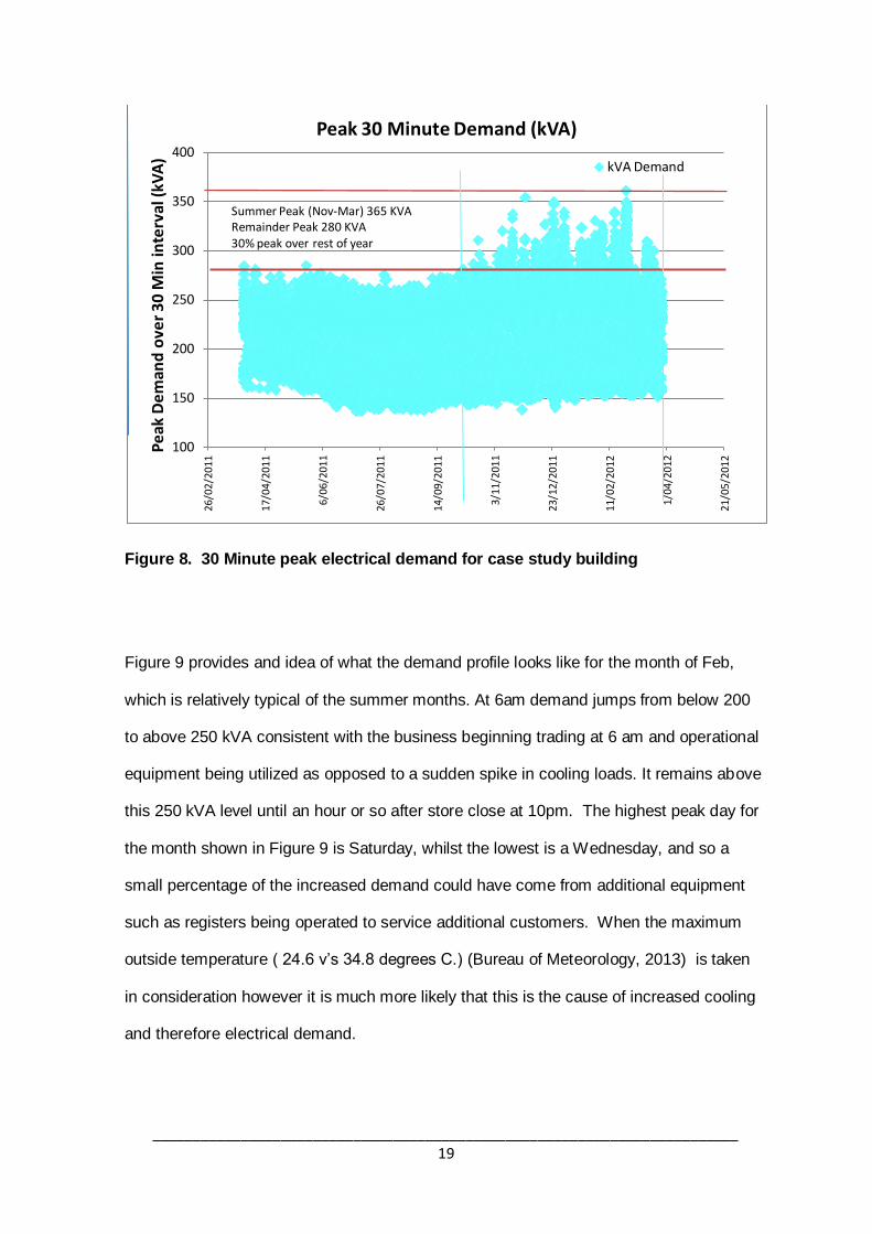
Figure 9 provides and idea of what the demand profile looks like for the month of Feb,
which is relatively typical of the summer months. At 6am demand jumps from below 200
to above 250 kVA consistent with the business beginning trading at 6 am and operational
equipment being utilized as opposed to a sudden spike in cooling loads. It remains above
this 250 kVA level until an hour or so after store close at 10pm. The highest peak day for
the month shown in Figure 9 is Saturday, whilst the lowest is a Wednesday, and so a
small percentage of the increased demand could have come from additional equipment
such as registers being operated to service additional customers. When the maximum
outside temperature ( 24.6 v’s 34.8 degrees C.) (Bureau of Meteorology, 2013) is taken
in consideration however it is much more likely that this is the cause of increased cooling
and therefore electrical demand.
100
150
200
250
300
350
400
26/0
2/2
01
1
17/0
4/2
01
1
6/06
/20
11
26/0
7/2
01
1
14/0
9/2
01
1
3/11
/201
1
23/1
2/20
11
11/0
2/20
12
1/04
/20
12
21/0
5/2
01
2 P
eak
De
man
d o
ver
30
Min
inte
rval
(kV
A)
Peak 30 Minute Demand (kVA)
kVA Demand
Summer Peak (Nov-Mar) 365 KVA Remainder Peak 280 KVA 30% peak over rest of year
_________________________________________________________________________ 20
Figure 9. Peak demand profile curves for Feb 2012
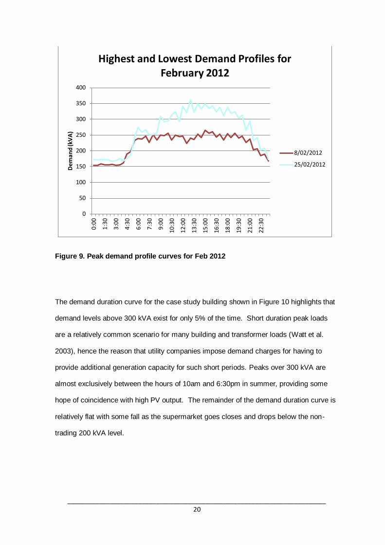
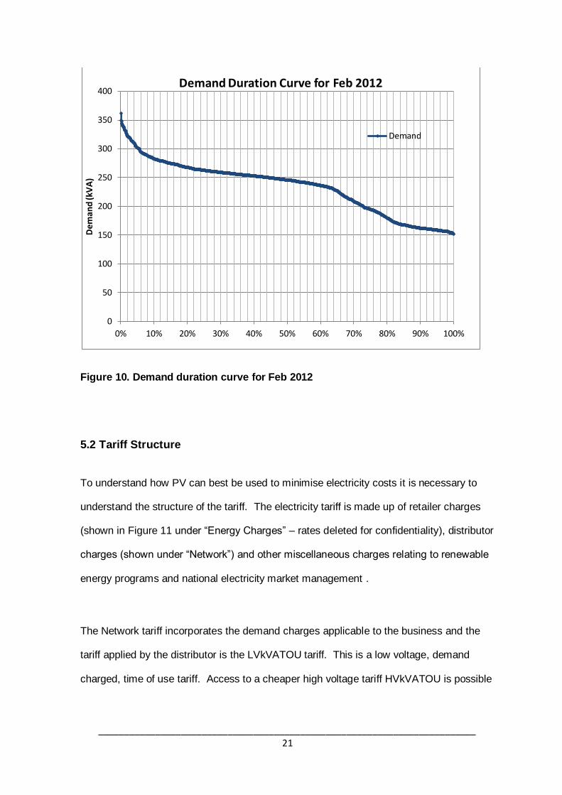
The demand duration curve for the case study building shown in Figure 10 highlights that
demand levels above 300 kVA exist for only 5% of the time. Short duration peak loads
are a relatively common scenario for many building and transformer loads (Watt et al.
2003), hence the reason that utility companies impose demand charges for having to
provide additional generation capacity for such short periods. Peaks over 300 kVA are
almost exclusively between the hours of 10am and 6:30pm in summer, providing some
hope of coincidence with high PV output. The remainder of the demand duration curve is
relatively flat with some fall as the supermarket goes closes and drops below the non-
trading 200 kVA level.
0
50
100
150
200
250
300
350
400 0:
00
1:30
3:00
4:30
6:00
7:30
9:00
10:3
0
12:0
0
13:3
0
15:0
0
16:3
0
18:0
0
19:3
0
21:0
0
22:3
0
De
man
d (k
VA
)
Highest and Lowest Demand Profiles for February 2012
8/02/2012
25/02/2012
_________________________________________________________________________ 21
Figure 10. Demand duration curve for Feb 2012
5.2 Tariff Structure
To understand how PV can best be used to minimise electricity costs it is necessary to
understand the structure of the tariff. The electricity tariff is made up of retailer charges
(shown in Figure 11 under “Energy Charges” – rates deleted for confidentiality), distributor
charges (shown under “Network”) and other miscellaneous charges relating to renewable
energy programs and national electricity market management .
The Network tariff incorporates the demand charges applicable to the business and the
tariff applied by the distributor is the LVkVATOU tariff. This is a low voltage, demand
charged, time of use tariff. Access to a cheaper high voltage tariff HVkVATOU is possible
0
50
100
150
200
250
300
350
400
0% 10% 20% 30% 40% 50% 60% 70% 80% 90% 100%
De
man
d (k
VA
) Demand Duration Curve for Feb 2012
Demand
_________________________________________________________________________ 22
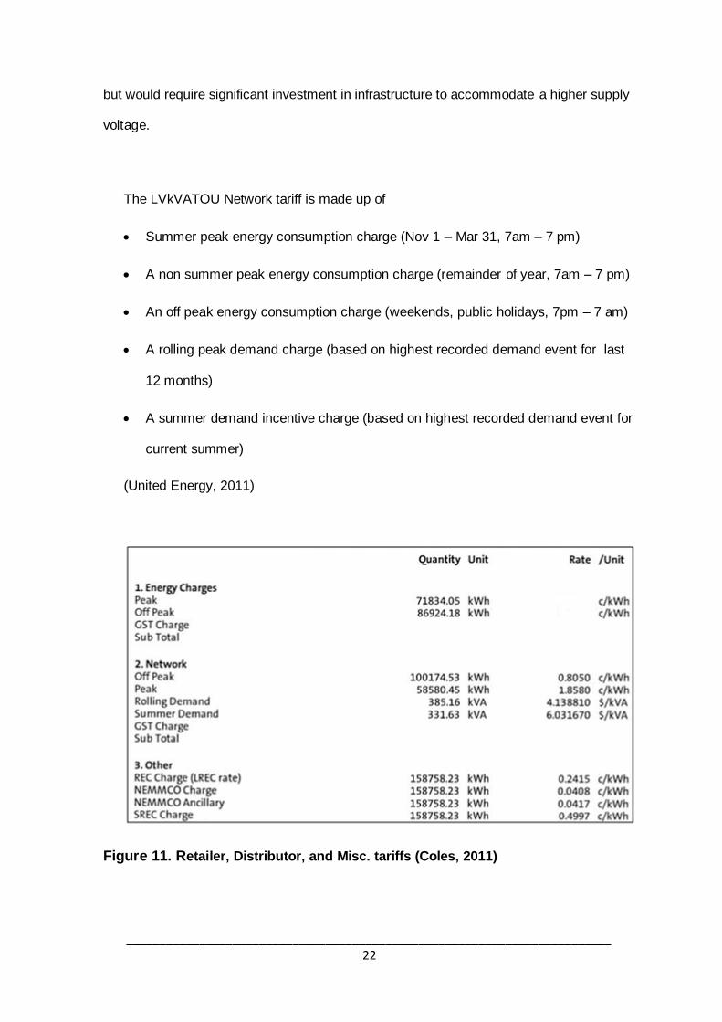
but would require significant investment in infrastructure to accommodate a higher supply
voltage.
The LVkVATOU Network tariff is made up of
Summer peak energy consumption charge (Nov 1 – Mar 31, 7am – 7 pm)
A non summer peak energy consumption charge (remainder of year, 7am – 7 pm)
An off peak energy consumption charge (weekends, public holidays, 7pm – 7 am)
A rolling peak demand charge (based on highest recorded demand event for last
12 months)
A summer demand incentive charge (based on highest recorded demand event for
current summer)
(United Energy, 2011)
Figure 11. Retailer, Distributor, and Misc. tariffs (Coles, 2011)
_________________________________________________________________________ 23
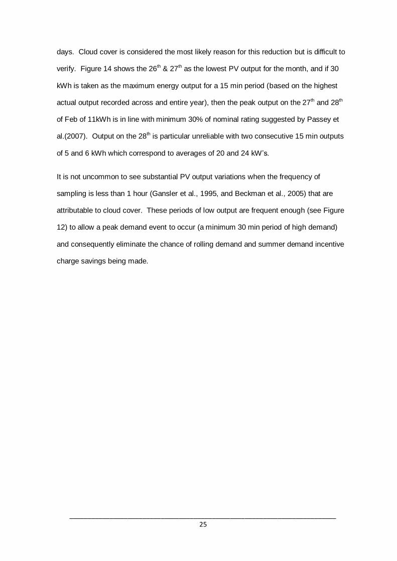
5.3 Solar PV data
The Queen Victoria Market PV system has a nominal size of 200 kW, although it is
suspected (based on conversations with the Melbourne City Council when sourcing the
data) that there are some faulty panels as there doesn’t seem to be a regular check of
system or individual panel output. Figure 12 below shows the energy output over 15 min
periods during February 2011 which corresponds with periods of high peak demand in the
case study building. Periods of zero output correspond with periods of darkness.
Fifteen minute energy output of approximately 30kWh corresponds to an average power
output of 120 kW which is significantly less than the 200 kW rated capacity. There are a
number of potential reasons for this loss, such as faulty panels, temperature effects, etc.
and it is something that would be worth investigating by Melbourne City Council given the
magnitude of the loss (estimates of losses for new systems are readily available from
suppliers). It is the reliability and timing of output however that is of interest in
determining the degree to which a PV system could offset peak demand. Figure 12
highlights some issues with the reliability of PV output (see 26th & 27th Feb) that are
discussed in more depth in the next section.
_________________________________________________________________________ 24
Figure 12. 15 min PV output Energy
5.4 Coincidence between PV output and Demand
For a PV system to be successful in offsetting peak demand it is important that there is a
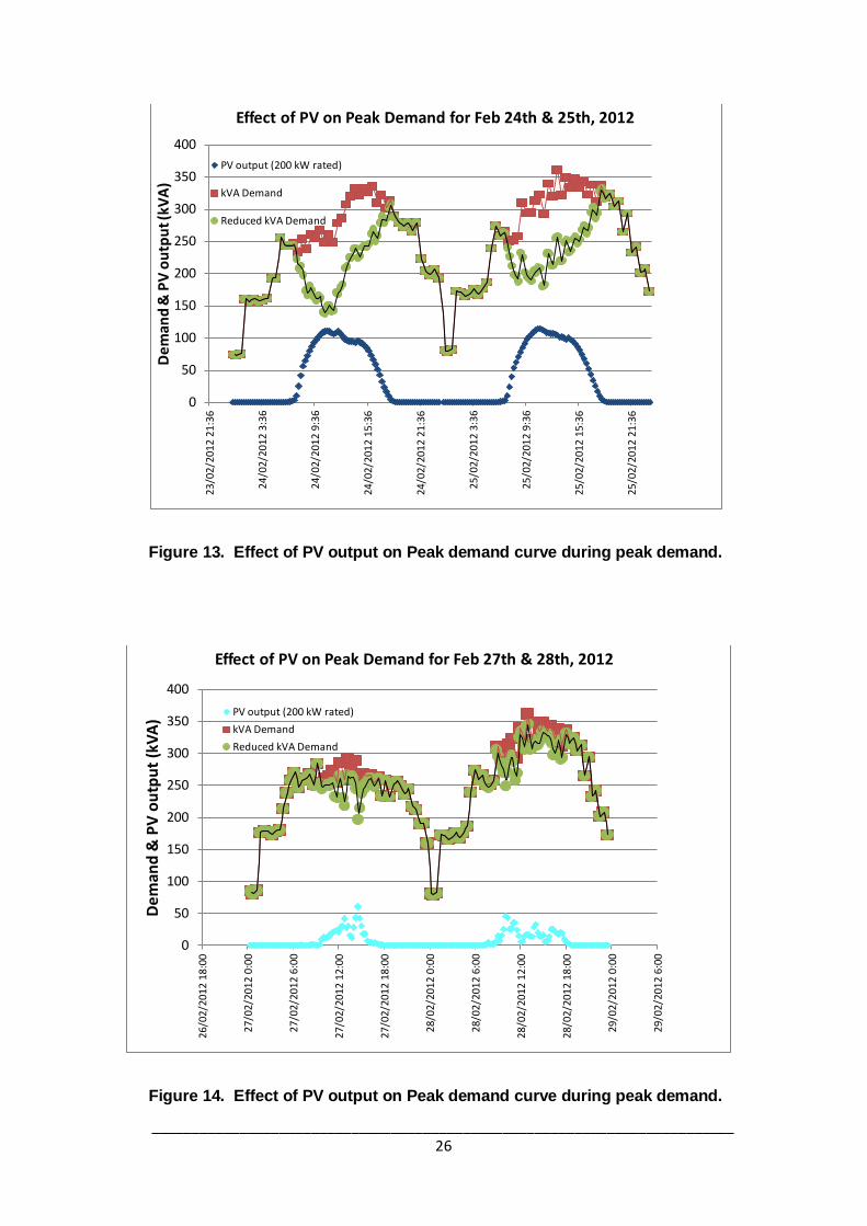
high degree coincidence in timing between the two events. Figure 13 shows that for the
24th & 25th of Feb, PV output peaks at approximately 11:00am (12 noon adjusting for
daylight savings) compared to demand peak levels between 1:00 and 4:00pm. The PV
peak could be delayed by rotating the array toward the west at the expense of annual
energy output (Watt et al, 1998).
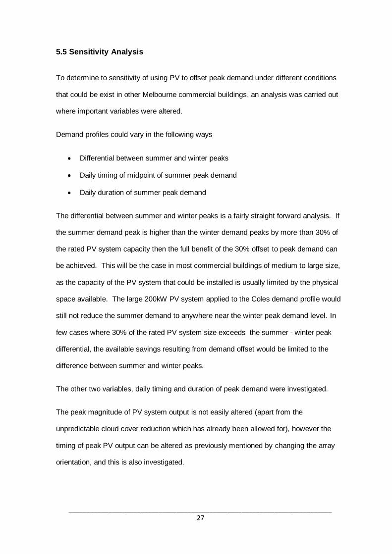
Figure 14 however shows that PV output can be dramatically different only a day later
with the system failing to produce a peak of more than about 50kW throughout either
0
5
10
15
20
25
30
35
1,-F
eb-1
1
1,-F
eb-1
1
2,-F
eb-1
1 3,
-Feb
-11
4,
-Feb
-11
5,
-Feb
-11
6,
-Feb
-11
7,
-Feb
-11
8,-F
eb-1
1
9,-F
eb-1
1
10-F
eb-1
1
11-F
eb-1
1
12-F
eb-1
1 13
-Feb
-11
14
-Feb
-11
15
-Feb
-11
16
-Feb
-11
17
-Feb
-11
18-F
eb-1
1
19-F
eb-1
1
20-F
eb-1
1
21-F
eb-1
1
22-F
eb-1
1 23
-Feb
-11
24
-Feb
-11
24
-Feb
-11
25
-Feb
-11
26
-Feb
-11
27-F
eb-1
1
15
min
PV
Ou
pu
t (k
Wh
)
Queen Vic PV System Output
Kwh
_________________________________________________________________________ 25
days. Cloud cover is considered the most likely reason for this reduction but is difficult to
verify. Figure 14 shows the 26th & 27th as the lowest PV output for the month, and if 30
kWh is taken as the maximum energy output for a 15 min period (based on the highest
actual output recorded across and entire year), then the peak output on the 27th and 28th
of Feb of 11kWh is in line with minimum 30% of nominal rating suggested by Passey et
al.(2007). Output on the 28th is particular unreliable with two consecutive 15 min outputs
of 5 and 6 kWh which correspond to averages of 20 and 24 kW’s.
It is not uncommon to see substantial PV output variations when the frequency of
sampling is less than 1 hour (Gansler et al., 1995, and Beckman et al., 2005) that are
attributable to cloud cover. These periods of low output are frequent enough (see Figure
12) to allow a peak demand event to occur (a minimum 30 min period of high demand)
and consequently eliminate the chance of rolling demand and summer demand incentive
charge savings being made.
_________________________________________________________________________ 26
Figure 13. Effect of PV output on Peak demand curve during peak demand.
Figure 14. Effect of PV output on Peak demand curve during peak demand.
0
50
100
150
200
250
300
350
400
23/0
2/2
01
2 2
1:3
6
24/0
2/2
01
2 3
:36
24/0
2/2
01
2 9
:36
24/0
2/2
01
2 1
5:3
6
24/0
2/2
01
2 2
1:3
6
25/0
2/2
01
2 3
:36
25/0
2/20
12 9
:36
25/0
2/20
12 1
5:36
25/0
2/20
12 2
1:36
De
man
d &
PV
ou
tpu
t (kV
A)
Effect of PV on Peak Demand for Feb 24th & 25th, 2012
PV output (200 kW rated)
kVA Demand
Reduced kVA Demand
0
50
100
150
200
250
300
350
400
26/0
2/20
12 1
8:00
27/0
2/20
12 0
:00
27/0
2/20
12 6
:00
27/0
2/20
12 1
2:00
27/0
2/20
12 1
8:00
28/0
2/20
12 0
:00
28/0
2/20
12 6
:00
28/0
2/20
12 1
2:00
28/0
2/20
12 1
8:00
29/0
2/20
12 0
:00
29/0
2/20
12 6
:00
De
man
d &
PV
ou
tpu
t (k
VA
)
Effect of PV on Peak Demand for Feb 27th & 28th, 2012
PV output (200 kW rated)
kVA Demand
Reduced kVA Demand
_________________________________________________________________________ 27
5.5 Sensitivity Analysis
To determine to sensitivity of using PV to offset peak demand under different conditions
that could be exist in other Melbourne commercial buildings, an analysis was carried out
where important variables were altered.
Demand profiles could vary in the following ways
Differential between summer and winter peaks
Daily timing of midpoint of summer peak demand
Daily duration of summer peak demand
The differential between summer and winter peaks is a fairly straight forward analysis. If
the summer demand peak is higher than the winter demand peaks by more than 30% of
the rated PV system capacity then the full benefit of the 30% offset to peak demand can
be achieved. This will be the case in most commercial buildings of medium to large size,
as the capacity of the PV system that could be installed is usually limited by the physical
space available. The large 200kW PV system applied to the Coles demand profile would
still not reduce the summer demand to anywhere near the winter peak demand level. In
few cases where 30% of the rated PV system size exceeds the summer - winter peak
differential, the available savings resulting from demand offset would be limited to the
difference between summer and winter peaks.
The other two variables, daily timing and duration of peak demand were investigated.
The peak magnitude of PV system output is not easily altered (apart from the
unpredictable cloud cover reduction which has already been allowed for), however the
timing of peak PV output can be altered as previously mentioned by changing the array
orientation, and this is also investigated.
_________________________________________________________________________ 28
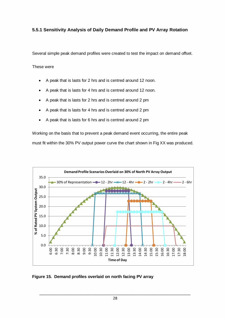
5.5.1 Sensitivity Analysis of Daily Demand Profile and PV Array Rotation
Several simple peak demand profiles were created to test the impact on demand offset.
These were
A peak that is lasts for 2 hrs and is centred around 12 noon.
A peak that is lasts for 4 hrs and is centred around 12 noon.
A peak that is lasts for 2 hrs and is centred around 2 pm
A peak that is lasts for 4 hrs and is centred around 2 pm
A peak that is lasts for 6 hrs and is centred around 2 pm
Working on the basis that to prevent a peak demand event occurring, the entire peak
must fit within the 30% PV output power curve the chart shown in Fig XX was produced.
Figure 15. Demand profiles overlaid on north facing PV array
0.0
5.0
10.0
15.0
20.0
25.0
30.0
35.0
6:0
0
6:3
0
7:0
0
7:3
0
8:0
0
8:3
0
9:00
9:3
0
10:0
0
10:3
0
11:0
0
11:3
0
12:0
0
12:3
0
13:0
0
13:3
0
14:0
0
14:3
0
15:0
0
15:3
0
16:0
0
16:3
0
17:0
0
17:3
0
18:0
0
% o
f R
ated
PV
Sys
tem
Ou
tpu
t
Time of Day
Demand Profile Scenarios Overlaid on 30% of North PV Array Output
30% of Representation 12 - 2hr 12 - 4hr 2 - 2hr 2 - 4hr 2 - 6hr
_________________________________________________________________________ 29
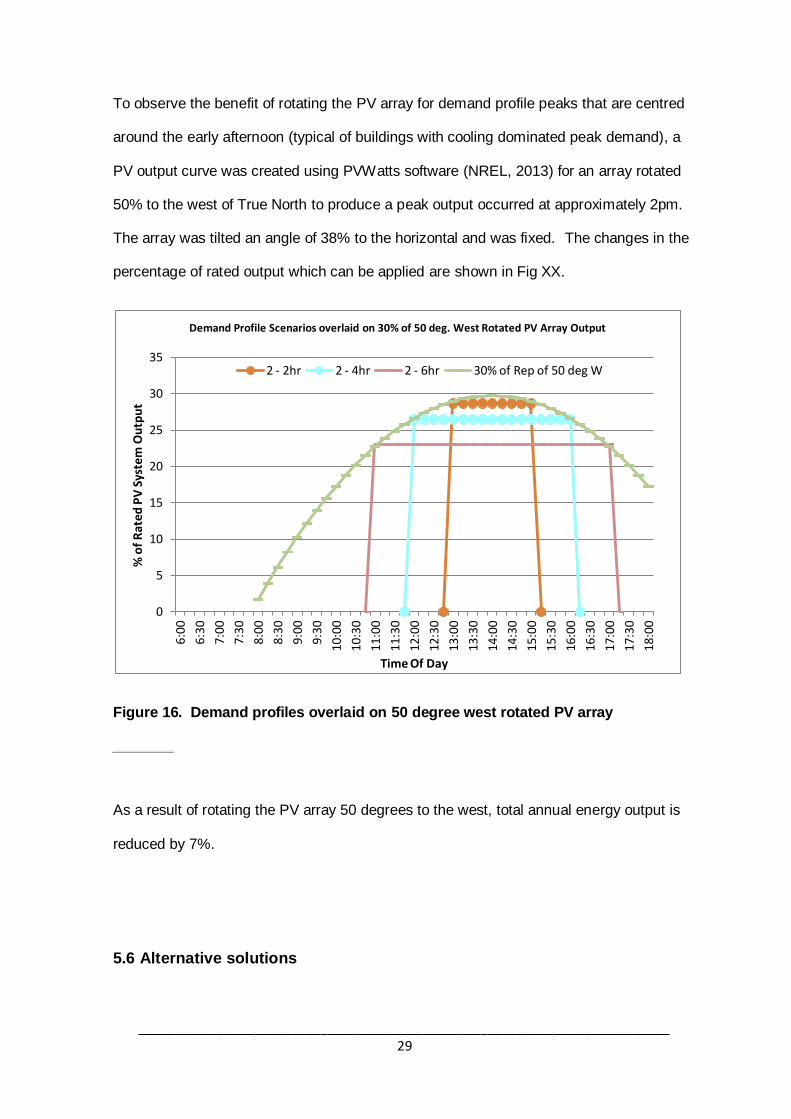
To observe the benefit of rotating the PV array for demand profile peaks that are centred
around the early afternoon (typical of buildings with cooling dominated peak demand), a
PV output curve was created using PVWatts software (NREL, 2013) for an array rotated
50% to the west of True North to produce a peak output occurred at approximately 2pm.
The array was tilted an angle of 38% to the horizontal and was fixed. The changes in the
percentage of rated output which can be applied are shown in Fig XX.
Figure 16. Demand profiles overlaid on 50 degree west rotated PV array
As a result of rotating the PV array 50 degrees to the west, total annual energy output is
reduced by 7%.
5.6 Alternative solutions
0
5
10
15
20
25
30
35
6:00
6:30
7:00
7:30
8:00
8:30
9:00
9:30
10:0
0
10:3
0
11:0
0
11:3
0
12:0
0
12:3
0
13:0
0
13:3
0
14:0
0
14:3
0
15:0
0
15:3
0
16:0
0
16:3
0
17:0
0
17:3
0
18:0
0
% o
f R
ated
PV
Sys
tem
Ou
tpu
t
Time Of Day
Demand Profile Scenarios overlaid on 30% of 50 deg. West Rotated PV Array Output
2 - 2hr 2 - 4hr 2 - 6hr 30% of Rep of 50 deg W
_________________________________________________________________________ 30
The following alternatives offer some potential solutions to the issue of unreliable PV
output.
5.6.1 Energy Storage
One potential solution is the use of some type of energy storage so that PV generated
energy can be stored for use when a peak demand event is about to occur. Onsite battery
storage is an obvious solution, but comes with cost, energy loss, space, and maintenance
considerations that will reduce the financial attractiveness of the total system. If we make
a few simple assumptions, the capacity of batteries required to ensure that 10 kVA could
be trimmed from peak demand for 3 consecutive days without any recharging is 4160 Ah
(at a system voltage of 48V). At a cost of approximately $0.20 / Wh (Batterystuff.com,
2013) the cost of batteries would be approximately $40,000 (see Appendix B for
calculations). Given the maximum achievable demand savings are $800 per annum (from
section 5.1) for a 10kVA reduction in peak demand, it is clear that such as storage system
is not going to be financially feasible in these circumstances.
Other forms of energy storage do exist (such as capacitors, flywheels, compressed air
systems etc) but factors such as cost, space and maintenance requirements generally
likely to make these alternatives less attractive than battery storage in most commercial
building environments.
5.6.2 PV Synched Demand Management.
Another alternative to maximise the available demand reduction available from PV is to
couple it with some demand management that is synchronised with PV output. In practice
this would involve throttling back systems such as air-conditioning or switching off
operating equipment for a period whilst PV output is reduced (e.g. due cloud cover).
Perez et al. (2003) found in a study of 3 buildings in the US, that the use of solar load
_________________________________________________________________________ 31
control (i.e. PV synched demand management) had the potential to be successfully
applied in commercial buildings most effectively through the reduction in building cooling
for a specified period of time. They found that a maximum allowance of 10 degree-hours
(eg 5 hrs at 2 degrees C above the normal cooling set point) per day above the standard
building temperature threshold, allowed combined synched cooling demand reduction and
PV to provide more than double the peak demand reduction of PV alone.
_________________________________________________________________________ 32
Chapter 6 – Financial Feasibility
6.1 Ideal theoretical maximum potential savings
To gain an idea of the maximum potential savings that could be made by offsetting
electricity consumption and demand charges a 12 month snapshot of data has been
selected to properly incorporate the effect of the 12 month rolling demand charges.
Tariff rates applicable at Dec 2011 were applied to the entire period.
For the purposes of simplification in this thesis, an approximation has been made in
equating the building electrical demand (measured in kVA) with real power (measured in
kW). The case study building has a high power factor (typically 0.92 to 0.96) meaning the
difference between the two quantities is relatively small, and allows for easier comparison
with PV system output.
As a starting point an ideal 10kW PV system was assumed to provide a full 10KVA
reduction to peak demand during the summer periods, and to provide a consumption
reduction of 1680 kWh per annum (based on an average of 4.6 Peak Sun Hours for
Melbourne).
This would provide total savings of approximately $2000 p.a. ($800 from demand
charges, and $1200 from consumption charges).
See Appendix A for calculations.
_________________________________________________________________________ 33
6.2 Practical potential savings
Despite occasional periods of low daily PV output during summer, the annual energy
output of a properly functioning PV system can be reasonably accurately predicted using
available software. Some organisations may consider a PV system financially feasible
based on energy savings alone. The intent of this research however is to determine
whether significant energy and peak demand savings can be made simultaneously.
To determine a practical level of demand charge savings, 30% of a rated PV system
output should be used in calculating an estimated demand charge saving. This would
reduce the estimated demand savings for the case study 10kW rated system from $800
p.a. to $240 p.a.
6.3 Available Government Rebates
There have been a number of programs created to provide incentives to both commercial
and residential customers to install PV and other renewable energy and energy saving
appliances. At present PV systems are currently eligible for Small Scale Technology
Certificates (STC’s) under the federal government’s Small Scale Renewable Energy
Scheme, when installed in accordance with the guidelines. The number of certificates is
dependent upon both the rated capacity of the system and the installed location (as this
will affect the total energy production expected from the system).
For example a 10kW system installed in the Melbourne region would attract around 177
STC’s (Clean Energy Regulator, 2013) which could be sold at the current price of
approximately $30 (totalling $5300) to offset the purchase cost of the system. These
schemes tend to undergo regular changes therefore current conditions should be verified.
_________________________________________________________________________ 34
6.4 PV System Costs
Outright purchase
The current cost of a mid range PV system (installed ) is approximately $2/watt (after the
benefit of STC’s) (Solar Choice, 2012) making the cost of a 10kW system approximately
$20,000 for outright purchase. An allowance of $5,000 has been made for cleaning and
inspection of the system over its lifetime, bring the total system cost to $25,000.
Alternatives exist to outright purchase, such as PV system lease plans, and Power
Purchase Agreements (PPA’s).
Leasing
PV system lease plans are very similar to the car lease plans that have been around for
many years. They involve an agreement to purchase PV generated electricity at set
prices (sometimes with inflation adjustments to price). They have the following benefits
Agreed purchase prices for electricity
No maintenance costs, ownership risks such as weather damage or performance
risk
Usually the option to purchase the system at the conclusion of the lease period for
a residual amount.
Power Purchase agreements
PPA’s are an agreement by a customer to purchase some or all of the power generated
by a PV system that is owned by a third party, for a specified period of time. They are
often used in large scale renewable energy projects but are now also available for small
scale PV systems. They have the following benefits:
No upfront capital investment
_________________________________________________________________________ 35
No maintenance costs, ownership risks such as weather damage or performance
risk
Allow businesses with insufficient space or inappropriate locations in which to
install PV panels to access the benefits of such systems.
Can lock in a fixed electricity purchase price for a number of years.
6.5 Financial Feasibility Indicators
There are a number of different measures for determining the financial feasibility of
projects, ranging from a simple Payback Periods and Return On Investment (ROI)
calculations, through to more detailed measures such as Levelised Cost. It has been
assumed that the customer has chosen to purchase a PV system outright.
Simple Payback period = Total cost of system / Annual savings
= $25,000 / $1845*
= 13.5 years
* A slightly adapted Annual Savings is used which is equal to the average yearly amount
saved across a 25 year lifespan with an assumed 2% increase in electricity costs per
annum. Assuming a 4% increase p.a. would give a simple payback period = 10.4 years
(See Appendix C). This method is used to provide some allowance for effect of
increasing electricity prices over 25 years.
A very rough guide to the Coles investment criteria for investment in energy efficiency
projects (provided in an email from Paul Lang of Coles on 23/08/12) is a payback period
of less than 4 years.
_________________________________________________________________________ 36
This means that using the metric of simple payback period, the use of a standalone PV
system to offset consumption and demand charges would not be considered feasible. It
would require forecast increase in annual electricity prices in the order of 10%, which is
well above current projections provided by AEMO (2012b) of 1-2% over the next 8 years.
A more sophisticated metric that takes into account factors such as the present value of
future costs and savings is the Levelised Cost of Electricity (LCOE). It is described in A
Manual for the Economic Evaluation of Energy Efficiency and Renewable Energy
Technologies, by Short et al. (1995) as
“a metric used to understand the per unit cost of the electricity generated by that system.
It is the cost that, if assigned to every unit of electricity produced by the system over its
lifetime will equal the net present value of the total lifetime system cost at the point of
implementation”
It is often used in renewable energy projects to determine whether over a certain duration
(such as 25 years in our case), the cost of the renewable energy is likely to be lower than
convention grid supplied electricity. It takes into account expenses such as capital,
maintenance and operating costs of the system over the selected duration, as well as the
discount rate (the amount by which future costs and income are adjusted to reflect their
value in today’s dollars) and the rate of increase of grid electricity prices. Whilst there is
some judgement involved in setting parameters such as the discount rate and electricity
price increases, it provides some guidance in comparing the cost of the different sources
of electricity. Using a discount rate of 4%, and a rate of increase of grid electricity prices
of 2% p.a. and a duration of 25 years (the remaining assumptions and calculator can be
seen in Appendix D) the following results are obtained.
Levelised cost of PV electricity = 11.3 cents / kWh
_________________________________________________________________________ 37
Levelised cost of Grid electricity = 13.2 cents / kWh
Whilst a detailed discussion of the calculation and implications of levelised cost
calculations are beyond the scope of this thesis, it suggests based on the provided
assumptions that a PV system would in fact be a cheaper way to meet some of the
consumption and demand requirements of the case study building over a 25 year period.
_________________________________________________________________________ 38
Chapter 7 – Discussion of results
7.1 Demand Observations
There is a high degree agreement between the reviewed literature and the results of
analysis of the case study data. Summer demand peaks are greater than in winter. Not
surprisingly however, supermarkets have a high proportion of cooling related demand
(55% refrigeration and 20% space cooling) (Department of Industry, Tourism, and
Resources, 2004) by comparison to the typical large office building average which is
around 40% (Australian Greenhouse Office, 2005) but can vary a bit depending on
climate. This helps explain the 30% differential in summer demand peaks compared to
winter, and why this differential is greater than the commercial sector average.
The demand duration curve for the case study was fairly consistent with other commercial
buildings (measured in literature via commercial transformer demand,) showing that for
February 2012 demand only exceeded 300 kVA (peaking at 350 kVA) for 5% of the time
(ie 14% of capacity is only required 5% of the time). What this curve doesn’t highlight is
that the peaks in demand (> 300 kVA) are usually sustained for several hours over a
limited number of summer days, as opposed to very short peaks experienced across a
number of days. This becomes evident when looking at daily demand profiles and is
consistent with demand being dominated by cooling loads in response to high
temperatures that begin around midday and last in the order of 4-8 hrs.
7.2 PV output observations
The coincidence in timing of peak demand and high PV output was reasonably good as
per previous commercial building case studies, with peak demand levels continuing for up
to a 2 or 3 hours after PV output had peaked. The timing of high PV output can be altered
_________________________________________________________________________ 39
to some degree by adjusting the orientation of the PV array toward the east or west , but
at the expense of total annual energy output.
When the case study PV output data was examined over a sub-daily period, it was
evident that the power output level which could be delivered with a high degree of
reliability was only in the order of 30% of system rated power. This was also in
agreeance with the literature, which attributed the low output primarily to cloud cover,
compounded in summer by further losses due to high PV module temperatures.
PV systems located north of Melbourne are typically going to deliver greater energy and
have less cloud cover annually, however unless there is a difference in the way peak
demand events are assessed by utility companies, the 30% estimate of high reliability PV
output would still be applicable as it only requires one cloudy day to potentially allow a
peak demand event to be recorded.
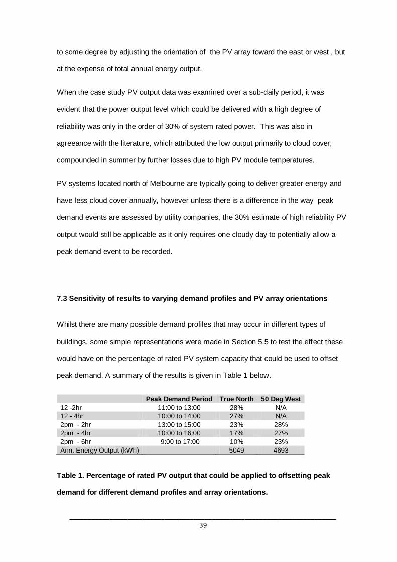
7.3 Sensitivity of results to varying demand profiles and PV array orientations
Whilst there are many possible demand profiles that may occur in different types of
buildings, some simple representations were made in Section 5.5 to test the effect these
would have on the percentage of rated PV system capacity that could be used to offset
peak demand. A summary of the results is given in Table 1 below.
Peak Demand Period True North 50 Deg West
12 -2hr 11:00 to 13:00 28% N/A
12 - 4hr 10:00 to 14:00 27% N/A
2pm - 2hr 13:00 to 15:00 23% 28%
2pm - 4hr 10:00 to 16:00 17% 27%
2pm - 6hr 9:00 to 17:00 10% 23%
Ann. Energy Output (kWh) 5049 4693
Table 1. Percentage of rated PV output that could be applied to offsetting peak
demand for different demand profiles and array orientations.
_________________________________________________________________________ 40
One finding is that there is significant benefit in rotating the PV array so that peak output
coincides approximately with the midpoint of peak demand. The benefit ranged from an
additional 20 - 130% increase in offsetable power, with forecast output in annual energy
output only falling by 7%. The biggest gain occurred where the demand peak was
prolonged (6 hr), as PV output falls away relatively quickly from its peak.
From a financial perspective the 7% fall in annual energy output ($87) would be
approximately equivalent to a 30% decrease in peak demand offset. This indicates that
an array rotation of 50 degrees to the west is warranted for both the 2pm midpoint – 4hr
duration and the 2pm midpoint – 6hr duration profile, for the tariff used in case study. An
easterly rotation was not modelled as it was considered unlikely that there would be many
buildings where the midpoint of summer demand occurred before midday, and
consequently a negative impact would occur on both demand and annual energy offset.
Further rotation to due west (90 degrees in total) shifts the peak PV output to closer to
3pm, with an annual energy output of 4017 kWh, a loss of approximately 20%. Given the
relatively small shift of 1 hour in the timing of peak output, compared to the additional 13%
decrease in annual energy output compared to the 50 degree rotation, it is considered
unlikely that the small saving in demand charges for profiles that peak late in the day,
would offset the rapidly declining annual energy loss.
7.4 Enhancements to PV system
Given 30% is a relatively low proportion of total PV rated power output, enhancement is
warranted to try and increase the feasibility of the system. Energy storage via batteries
was investigated and whilst it is well proven technically, it is a fair way from being
financially viable in a peak demand offset scenario. Other energy storage devices exist
but are generally likely to be less attractive due to one of more factors including cost,
physical space requirement, maintenance, and technical complexity.
_________________________________________________________________________ 41
PV synched demand management was identified from existing literature as a possible
solution with cooling related demand targeted as an area that could provide the required
reduction at critical times. This could be trialled in many commercial buildings such as
offices where the impact is a small change in the occupant comfort level, that is unlikely to
cause financial loss (at least for the trial duration). In the case of a supermarkets, further
investigation would be required to determine the impact of reduced cooling on product
quality and life, as there is potential for significant financial loss through spoilt product,
particularly in fruit and veg. sections where produce is often stored outside of refrigeration
bays, relying on building space cooling for preservation. Another factor to be taken into
consideration is that in an office building the occupants have no choice with regard to
relocating to another cooler building (at least in the short term) whereas supermarket
customers may display a preference to shop elsewhere in a cooler environment.
A feature that has already been identified as having the greatest potential for electricity
consumption ( and quite likely demand) reduction, are air locks at store entrances, to
prevent the escape of cooled air (Department of Industry, Tourism, and Resources,
2004). This feature stands to produce greater savings where customers enter from the
external environment versus from within a shopping complex. It could however be a
valuable exercise to estimate to what degree supermarket cooling, (which in the author’s
experience is generally to a lower temperature than the shopping complex because of
produce preservation requirements) supplements cooling in the remainder of the complex,
where the store has a large open frontage.
Another enhancement that could assist is demand management in buildings with high
cooling loads is thermal storage within the building’s cooling systems. There have already
been successful applications of chilled water and an ice storage unit within universities in
Australia (Bahnfleth et al., 2003), that effectively store cooling capacity during off peak
periods when the cost of energy is low, and there is no risk of creating a peak demand
event. The stored cooling capacity is then discharged during periods of peak electricity
_________________________________________________________________________ 42
demand, thereby reducing the peak demand, and minimising electricity consumption
during higher cost peak periods. The economics of scaling this system up or down in size
to suit individual building demand, maintenance, and physical space requirements would
need to be considered in each application.
7.5 Technical Feasibility Result
From a technical perspective there aren’t any show stopping issues that would prevent a
standalone PV system from being used in the case study to offset peak demand and
consumption charges. This can be extended generally to other commercial buildings
provided the physical space for the PV array is available in location such that an
unshaded northerly orientation can be achieved.
7.6 Financial Feasibility Result
One of the challenges immediately apparent when reviewing the case study tariff data is
that the unit cost of electricity (cents / kWh) (factoring in both demand and consumption
charges) is relatively low by comparison to the typical price that residential customers
pay. For the month of December 2011, the average unit cost of electricity for the case
study building, taking into account both consumption and demand charges, was around
10.5 cents / kWh, compared to a cost of 20-22 cents for residential customers(Ausgrid,
2012). Whilst January and February 2011 average electricity costs for the case study
were likely a little higher than 10.5 cents due to higher cooling demand, the yearly
average would not be expected to be any greater than this. Other commercial buildings
with similar annual consumption levels may in fact have lower average electricity costs, as
their demand across the year is usually a little more uniform than for supermarkets
(SEAV, 2004), and hence demand charges will add less to the annual average unit cost.
_________________________________________________________________________ 43
Looking at the simple metric that Coles have supplied where the Simple Payback Period
must be less than 4 years, it is obvious that the neither the standalone PV system or an
enhanced version with battery storage, are going to be considered financially feasible. An
assessment using the Levelised Cost of Electricity however gives a slightly different
perspective, one that suggests over the life of the PV system, that it may in fact deliver
cost savings. This metric is sensitive to the choice of discount rate (often a contentious
issue) and to the forecast increase in electricity prices, and therefore the decision on
financial feasibility may depend to a large degree on individual business preferences in
determining these values.
Looking at the range of tariffs imposed by the distributor (United Energy, 2011) there is
some evidence of an inverse relationship between the amount of consumption and the
unit cost of demand charges. This may mean that some of the strategies investigated to
reduced demand charges may perform better in buildings with lower annual energy
consumption (<400 MWh p.a.) but which still have demand charges as part of their tariff.
Further Information regarding consumption charges for smaller commercial consumers
would be required before drawing any further conclusions.
_________________________________________________________________________ 44
7.7 Limitations of Results
The applicability of some aspects of these results to other commercial buildings will be
dependent on the type of building and the nature of the business being carried out.
Commercial buildings with relatively low cooling demand may find that their peak demand
arises largely from other sources such as process equipment, and that this combined with
increased lighting requirements in winter could result in peak demand events occurring at
time when PV output is quite limited.
Different tariffs applied by other retailers and distributors in other locations will naturally
influence financial feasibility and these should be allowed for, however the majority of
findings are still applicable. Similarly geographic location will affect the annual energy
output of a PV system to a degree, and this should be adjusted for when estimating
savings.
_________________________________________________________________________ 45
Chapter 8 – Conclusion
An investigation into the feasibility of using solar PV to reduce demand and consumption
charges in commercial buildings in Melbourne has produced some interesting conclusions
that are generally in keeping with existing literature on the subject.
PV systems as a standalone option can only reliably provide a maximum of 30% of their
rated capacity toward offsetting peak demand events due largely to the risk of cloud cover
reducing their output during a peak demand period.
Whilst a higher coincidence exists between the timing of peak demand events and high
PV output in commercial buildings compared to residential, the timing is still not optimal
for a north facing array which would maximise annual energy consumption. If peak
demand occurs in the early afternoon as would be expected when demand is driven by
cooling and/or operating hours that extend past normal business hours, then an array
rotation to the west (up to approx. 70 degrees) is likely to provide an increase in peak
demand offset, and overall greater cost savings. The case study building demonstrated
high demand peaks that were centred around 2pm, and would therefore benefit from an
array rotation of approximately 50 degrees to the west.
Standalone PV systems whilst technically feasible in offsetting peak demand and
consumption charges (providing space and orientation requirements can be met), struggle
when it comes to financial feasibility. Relatively low demand and consumption charges (by
comparison to residential rates), and the low level of usable rated PV capacity in offsetting
peak demand events, mean PV systems at current prices have substantial payback
periods that will often be beyond the threshold for investment set by many businesses.
The Levelised Cost of Electricity provides a more sophisticated approach to determining
financial feasibility and it is recommend that this should be carried out to provide an
alternative perspective when assessing projects of this nature.
_________________________________________________________________________ 46
Enhancements to a standalone system in the form of energy storage via battery banks
was also not viable due to the cost of significant storage capacity required to prevent a
peak demand event occurring over a period of up to 3 days with cloud cover.
Where cooling represents a large proportion of summer peak demand, there is the
opportunity to reduce demand by raising cooling system set points for a short period
without significantly disrupting business activities in many types of buildings, to coincide
with short periods of reduced PV system output. Exceptions to this would include
buildings where internal temperature control has a material effect on business product,
processes, or persons who are more sensitive to the effects of high temperatures such as
those in hospitals or the elderly.
One area where further work could improve the value of a PV system in offsetting peak
demand, is in investigating the response to a small short term rise in internal building
temperatures as a result PV synched cooling demand reduction. Determining which types
of commercial buildings and businesses are suited to this and the degree to which it can
be implemented would be useful in assessing the benefits of this strategy.
In conclusion, commercial buildings that are best suited to PV demand offset are those
where
summer demand peaks that are greater than winter
demand peaks have their midpoint between midday and 3pm (and a suitable array
orientation is possible)
demand peaks have durations of 4hrs of less
the applicable tariff includes rolling (annual) and summer demand charges, and
cooling related demand exists and a small degree of demand management will not
significantly affect product or occupants
_________________________________________________________________________ 47
References
ABARE , 2011, Australian Energy Statistics - Energy update 2011, accessed online on 02/01/03 at
http://www.daff.gov.au/abares
Ausgrid, 2012, Residential electricity prices and energy bills 2011/12 – Sydney vs Melbourne,
accessed online 01/02/2013 at
http://www.ausgrid.com.au
Australian Energy Market Operator (AEMO) 2012a, “ECONOMIC OUTLOOK
INFORMATION PAPER, National Electricity Forecasting” accessed online 6/8/2012 at
http://www.aemo.com.au/Electricity/~/media/Files/Other/forecasting/Economic_Outlook_Informa
tion_%20Paper.ashx
Australian Energy Market Operator (AEMO) 2012b, National Electricity Forecasting Report (NEFR)
2012, accessed online 6/10/2012 at
http://www.aemo.com.au/Electricity/Planning/Forecasting/National-Electricity-Forecasting-
Report-2012
Australian Energy Regulator, 2009, State of the Energy Market 2009, accessed online at
http://www.aer.gov.au/sites/default/files/Chapter%201%20Electricity%20generation%202009.pd
f
Australian Greenhouse Office, 2005, Office Building Energy Use, accessed online 8/12/12
at http://yourbuilding.fusion.com.au/Article/NewsDetail.aspx?p=83&id=1596
Bahnfleth. W., Graeme. R., McLeod. S., Bowins, L., 2003, Chilled Water Storage in
Western Australia, ASHRAE Transactions: Symposia
_________________________________________________________________________ 48
Batterystuff.com, 2013. Solar Photovoltaic (PV) Batteries for Home, RV and Backup
Systems , accessed online on 4/01/13 at http://www.batterystuff.com
Beckman. W, Vijayakumar.G, Kummert.M, Klein, S, Analysis of short-term solar
radiation data,Solar Energy 79 (2005) 495–504
Bureau of Metrology, 2013, Historical Weather Data, accessed online on 12/9/12 at
www.bom.gov.au
Centre for International Economics, 2007, Capitalising on the building sector’s potential to
lessen the costs of a broad based GHG emissions cut, accessed online on 7/12/12 at
http://www.asbec.asn.au/files/Building-sector-potential_Sept13.pdf
Clean Energy Regulator, 2013. Small Generation Unit STC Calculator, accessed online
on 10/01/13 at https://www.rec-registry.gov.au/sguCalculatorInit.shtml
Coles, 2011, e-mail to author, May 2012
Department of Industry, Tourism, and Resources, 2004, Greening of Coles Case Study
Accessed online 6/10/2012 at
_________________________________________________________________________ 49
http://buildgreen.co.nz/projects/eebp-coles/Coles_case_study20040907111052.pdf
Dept. Resources, Energy & Tourism, 2011, Energy in Australia 2011, accessed online at
http://adl.brs.gov.au/data/warehouse/pe_abares99001789/Energy_in_Aust_2011_13f.pdf
Dunstan. C, 2008, Win, Win, Win: Regulating Electricity Distribution Networks for
Reliability, Consumers and the Environment – Review of the NSW D-Factor and
Alternative Mechanisms to encourage Demand Management, Institute for Sustainable
Futures, University of Technology Sydney for the Total Environment Centre
Energy Australia, 2005, Kogarah Town Square Photovoltaic Power System – Demand
Management Analysis, for the NSW Department of Planning
Gellings.C, 1981- A phrase coined by Clarke Gellings.
Gansler.R, Klein.S, and Beckman.W, Investigation of minute solar radiation data.
Solar Energy Vol. 55, No. 1, pp. 21-27, 1995
GTM Research, 2013. Solar module price forecasts lowered to 42c/watt, Renew
Economy, access online 4/01/2013 at
http://reneweconomy.com.au/2013/solar-module-price-forecasts-lowered-to-42cwatt-53901
Gyamfia, S. Krumdieck, S (2012). Scenario analysis of residential demand response at
network peak periods, Electric Power Systems Research 93 (2012) 32– 38
_________________________________________________________________________ 50
Hope, G., R. Schoettle, et al. 2000. "Operation Review of June 14, 2000 PG&E Bay area
system events using Aempfast Software: final report.” Benicia, CA
Melbourne Energy Institute, 2011 “Renewable Energy Technology Cost Review”, pg 2,
accessed online 6/8/2012 at
http://www.garnautreview.org.au/update-2011/commissioned-work/renewable-energy-
technology-cost-review.pdf
National Renewable Energy Laboratory (NREL), 2013, PVWatts Software, accessed
online 2/3/13 at http://rredc.nrel.gov/solar/calculators/pvwatts/version1/
Passey, R., Watt, M., Outhred, H., Spooner, T. and Snow, M., 2007, Study of Grid
connect Photovoltaic Systems - Benefits, Opportunities, Barriers and Strategies, for
The Office of Energy, Western Australian Government.
Rowlands, I.H.,2005 Solar PV Electricity and market characteristic: Two Canadian case
studies. Renewable Energy, 30 (6), pp. 815-834
Shugar, D. S., 1990. "Photovoltaics in the Utility Distribution System: The Evaluation of
System and Distribution Benefits. Proceedings of the 21st IEEE Photovoltaics
Specialists Conference." Kissimmee, Florida.
Solar Choice, 2012. 10kW solar power systems: Price, power output, and returns. .
_________________________________________________________________________ 51
Accessed 21/10/2012 online at http://www.solarchoice.net.au/
Stadler, I. 2007. "Power Grid Balancing of Energy Systems with High Renewable
Energy Penetration by Demand Response " Journal of Utilities Policy 16(2): 90-98.
Steinfeld.J, Bruce.A, Watt.M, Peak load characteristics of Sydney office buildings and
policy recommendations for peak load reduction, Energy and Buildings, Volume 43,
Issue 9, September 2011
Sustainable Energy Authority of Victoria (SEAV) 2004, The impact of Commercial and
Residential sectors’ EEIS on electricity demand, accessed on 02/01/13 at
http://www.ret.gov.au/Documents/mce/energy-eff/nfee/_documents/consreport_07_.pdf
United Energy 2011, UE Tariff Schedule 2011, Accessed 01/04/2012 at
http://www.unitedenergy.com.au/media/8325/2011_tariff_schedule.pdf
US Dept. Of Energy, 2012. US Energy Information Administration – Independent statistics
and analysis. Accessed 21/10/2012 at
http://www.eia.gov/cfapps/ipdbproject/iedindex3.cfm
Watt, M., Kaye, J., Travers, D., MacGill, I., Prasad, D., Thomas, P.C., Fox, E., Jansen, S.,
1998, Opportunities for the Use of Building Integrated Photovoltaics in NSW, Report to
SERDF,
Watt.M, Outhred.H, Spooner.T, MacGill.I, Oliphant.M, Partlin.S, 2005, Photovoltaics and
Peak Electricity Loads - Summer 2003-04, Centre for PV Engineering UNSW, for BP
Solar, Origin Energy and the Sustaiable Energy Authority of Victoria
_________________________________________________________________________ 52
Watt.M, Passey.R, Parker.F, Rivier.J, 2006, Newington Village, An Analysis of
Photovoltaic Output, Residential Load and PV’s Ability to Reduce Peak Demand,
Centre for Energy & Environmental Markets, for the NSW Department of Planning.
Watt.M, Passey.R, and Snow.M, (2007), “The Contribution of Photovoltaics to
Commercial Loads” , School of Photovoltaic and Renewable Energy Engineering,
University of New South Wales
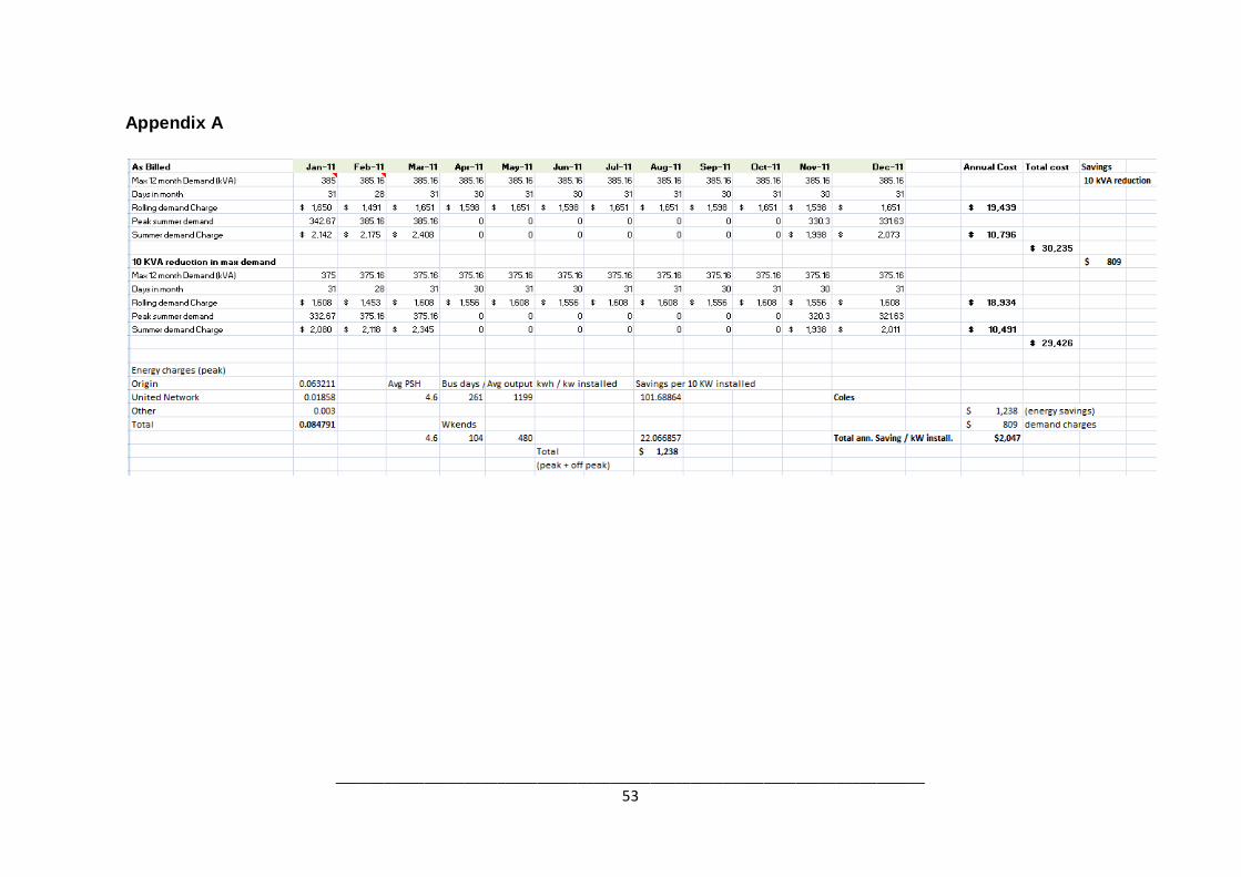
_________________________________________________________________________ 53
Appendix A
Coles
$ 1,238 (energy savings)
$ 809 demand charges
Total ann. Saving / kW install. $2,047
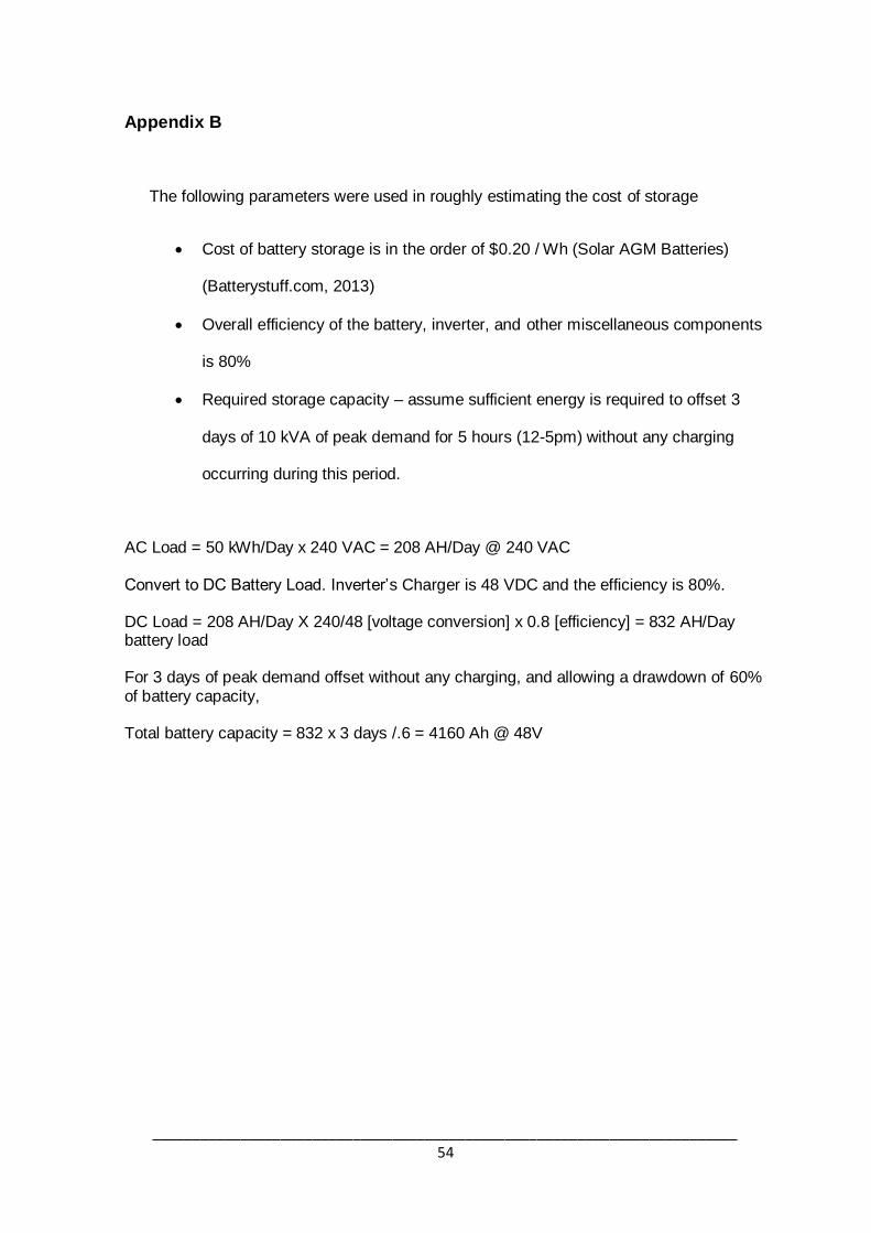
_________________________________________________________________________ 54
Appendix B
The following parameters were used in roughly estimating the cost of storage
Cost of battery storage is in the order of $0.20 / Wh (Solar AGM Batteries)
(Batterystuff.com, 2013)
Overall efficiency of the battery, inverter, and other miscellaneous components
is 80%
Required storage capacity – assume sufficient energy is required to offset 3
days of 10 kVA of peak demand for 5 hours (12-5pm) without any charging
occurring during this period.
AC Load = 50 kWh/Day x 240 VAC = 208 AH/Day @ 240 VAC Convert to DC Battery Load. Inverter’s Charger is 48 VDC and the efficiency is 80%. DC Load = 208 AH/Day X 240/48 [voltage conversion] x 0.8 [efficiency] = 832 AH/Day battery load For 3 days of peak demand offset without any charging, and allowing a drawdown of 60% of battery capacity, Total battery capacity = 832 x 3 days /.6 = 4160 Ah @ 48V
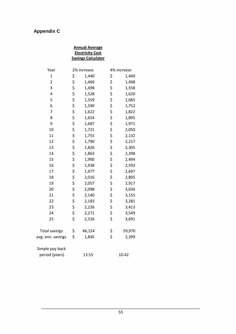
_________________________________________________________________________ 55
Appendix C
Annual Average Electricity Cost
Savings Calculator
Year 2% increase 4% increase 1 $ 1,440 $ 1,440 2 $ 1,469 $ 1,498 3 $ 1,498 $ 1,558 4 $ 1,528 $ 1,620 5 $ 1,559 $ 1,685 6 $ 1,590 $ 1,752 7 $ 1,622 $ 1,822 8 $ 1,654 $ 1,895 9 $ 1,687 $ 1,971 10 $ 1,721 $ 2,050 11 $ 1,755 $ 2,132 12 $ 1,790 $ 2,217 13 $ 1,826 $ 2,305 14 $ 1,863 $ 2,398 15 $ 1,900 $ 2,494 16 $ 1,938 $ 2,593 17 $ 1,977 $ 2,697 18 $ 2,016 $ 2,805 19 $ 2,057 $ 2,917 20 $ 2,098 $ 3,034 21 $ 2,140 $ 3,155 22 $ 2,183 $ 3,281 23 $ 2,226 $ 3,413 24 $ 2,271 $ 3,549 25 $ 2,316 $ 3,691
Total savings $ 46,124 $ 59,970 avg. ann. savings $ 1,845 $ 2,399
Simple pay back period (years) 13.55 10.42
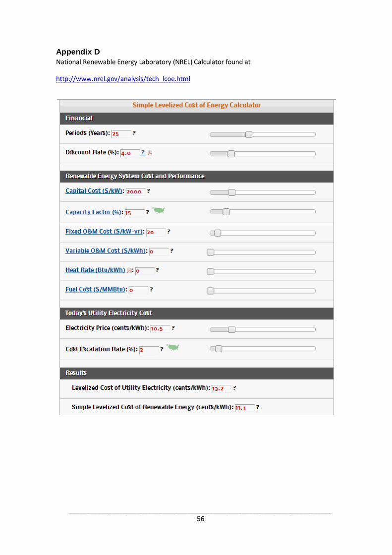
_________________________________________________________________________ 56
Appendix D
National Renewable Energy Laboratory (NREL) Calculator found at
http://www.nrel.gov/analysis/tech_lcoe.html
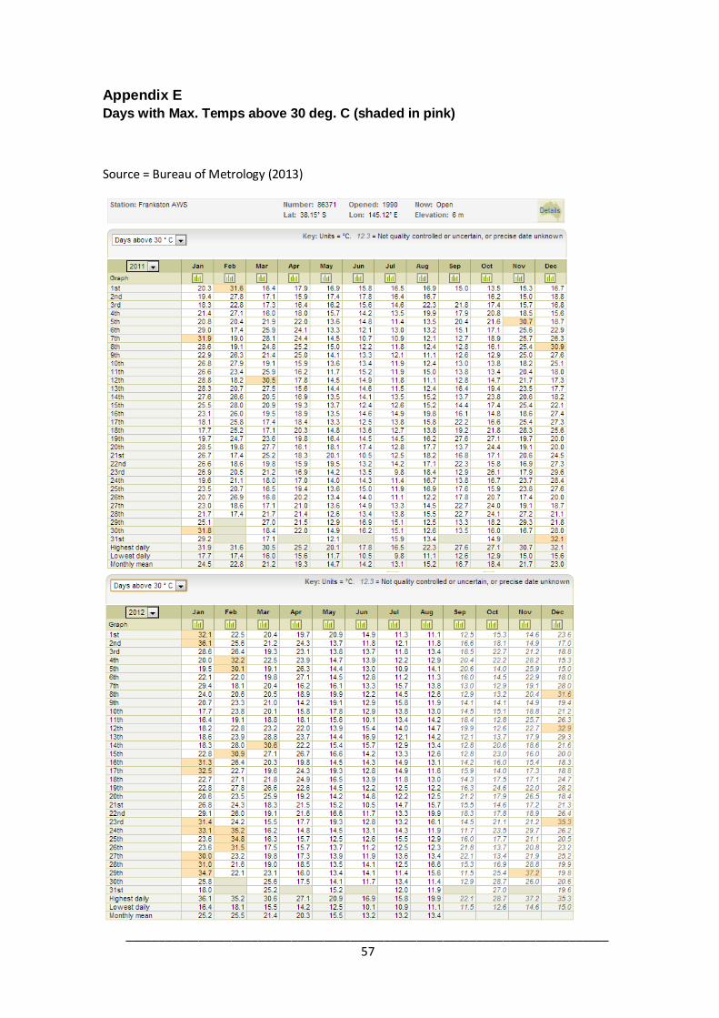
_________________________________________________________________________ 57
Appendix E
Days with Max. Temps above 30 deg. C (shaded in pink)
Source = Bureau of Metrology (2013)