Annual Report(2004) Kawahara Lab.

A Fictitious Domain Methodwith The Distributed Lagrange Multiplier

for Particulate Flow

M. Nagai and M. Kawahara

Department of Civil Engineering, Chuo University,

Kasuga 1-13-27, Bunkyou-ku, Tokyo 112-8511, JAPAN

E-mail:motoyuki@kc.chuo-u.ac.jp

Department of Civil Engineering, Chuo University,

Kasuga 1-13-27, Bunkyou-ku, Tokyo 112-8511, JAPAN

E-mail:kawa@kc.chuo-u.ac.jp

ABSTRACT

In this article the numerical simulation of incompressible viscous flow around a blow upparticle is discussed. The rigid particle motions in the fluid are caused by fluid forces andgravity. The incompressible Navier-Stokes equation and Newton law are introduced as thebasic equation showing fluid flow and action of a rigid body particle, respectively. To solvethis problem, the finite element method and the fictitious domain method with distributedlagrange multiplier are applied. In case of the fictitious domain method, the method is notnecessary to remeshing. Therefore, in case of the complicated and large-scaled computationalmodel, it can be solved quickly.

KEY WORDS

finite element method, fictitious domain method, distributed lagrange multiplier, Navier-Stokes equations, New-ton law

INTRODUCTION

The fluid-body coupled analysis exists in the field of engineering. Even if it restricts to the field of civilengineering, such as beach drifting, scouring around the pier and sedimentation of the sand at the river mouthexist. These problems are caused by the force which a particle receives from fluid (fluid force) or change of theeffective stress between the particles accompanying change to the pressure in fluid. These problems do a lotof damage to our life. Thus, the fluid-body coupled analysis is an important problem in the field of naturalenvironment and engineering. This research shows blow up particle model which exist in the fluid-body coupledanalysis.

In recent years, the finite element analysis carried out rapid development. As finite element analysis devel-oped rapidly, complicated and large-scaled model containing the moving boundary and body are increased. Butcomputation of such model arise many problems. The conventional finite element method had to be remeshto adjust the transformation of the computation domain in the moving boundary problem. Thus, computationof complicated and large-scaled model arise shortage of memory and increase of computational time since fornecessity of remeshing. On the other hand in case of the fictitious domain method, two kind of finite element

158

meshes are used. One is the small mesh for moving particle, the other is the large mesh for whole computationaldomain. In the moving particle problem, the small mesh can move on a large the mesh without fitting a node.In the conventional finite element method, node and moving boundary had to be fit and remeshing is neededin each time step. In each time step remeshing is needed. The fictitious domain method is not necessary toremesh. Therefore, we can save memory amount and computational time can become shorter.

In this research, to test of the efficiency of the fictitious domain method for particle flows, a two-dimensionalflow with blow up particle is simulated.

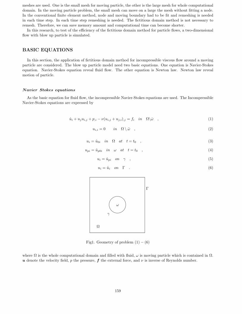
BASIC EQUATIONS

In this section, the application of fictitious domain method for incompressible viscous flow around a movingparticle are considered. The blow up particle model need two basic equations. One equation is Navier-Stokesequation. Navier-Stokes equation reveal fluid flow. The other equation is Newton law. Newton law revealmotion of particle.

Navier Stokes equations

As the basic equation for fluid flow, the incompressible Navier-Stokes equations are used. The IncompressibleNavier-Stokes equations are expressed by

ui + ujui,j + p,i − ν(ui,j + uj,i),j = fi in Ω\ω , (1)

ui,i = 0 in Ω \ ω , (2)

ui = u0i in Ω at t = t0 , (3)

upi = up0i in ω at t = t0 , (4)

ui = upi on γ , (5)

ui = ui on Γ . (6)

ω

γ

Ω

Γ

Fig1. Geometry of problem (1)− (6)

where Ω is the whole computational domain and filled with fluid, ω is moving particle which is contained in Ω.u denote the velocity field, p the pressure, f the external force, and ν is inverse of Reynolds number.

159

Newton law

The particle motions are caused by fluid force and gravity. then the motion of the particle follows themomentum equations given by the Newton law,

mpdvp

dt= (1− ρf

ρp)mpg + F p , (7)

Ipdωp

dt= T p , (8)

dGp

dt= vp . (9)

where vp is the translation velocity of the particle, ωp is the angular speed of the particle, mp is the mass of theparticle, Ip is the moment of inertia of the particle, Gp is the center of the particle, g is the gravity, ρp is thedensity of the particle, F p is the force imposed on the particle by the fluid, Tp is the moment imposed on theparticle by the fluid. The force and the moment imposed on the particle by the fluid are described as follows,

F p =∫

γ

σndx , (10)

T p =∫

γ

(x− Gp)× (σn)dx . (11)

where σ = −pI + ν(∇u + ∇uT ) is stress tensor, x is the generic point and n is the pointing outward unitnormal vector on γ.

The velocity of the particle and the center of the particle is computed as follows,

vpn+1 = vp

n +∆t(1− ρf

ρp)g +∆t

F np

mp, (12)

wpn+1 = wp

n +∆tTp

n

Ip, (13)

Gpn+1 = Gp

n +∆tvnp . (14)

From the above equations, total velocity of the particle is obtained as follows,

un+1 = vpn+1 + wp

n+1 × (xn+1 − Gpn+1) on γ . (15)

Collision

In this research, collision between particles and wall are also considered. Considering the collisions betweenparticles and wall, the following equation is used instead of the momentum equation(7).

mpdvp

dt= (1− ρf

ρp)mpg + F p + F c

p , (16)

160

where F cp is an impulsive force imposed on the particle by the other particles or the walls. The impulsive

force F cp is defined as follows,

F cp = F w

p + F pp , (17)

where F wp is impulsive force between the particle and the wall and F p

p is the impulsive force between particles.The impulsive force is hard to calculate directly. Therefore in order to calculate the impulsive force, threeequations are introduced as follow,

mp(va(t2) + vb(t2) ) = mp(va(t1) + vb(t1) ) , (18)

e = −va(t2)− vb(t2)va(t1)− vb(t1)

, (19)

∫ t2

t1

F cpdt = mp

∫ t2

t1

dv

dtdt = mpv(t2)−mpv(t1) . (20)

where e is repulsion coefficient.

In order to judge the touch between the particles and calculate the impulsive force, the short range is set betweenthe particles or the wall. Because mesh for particle is not allowed to overlap the each other and go through thewall.

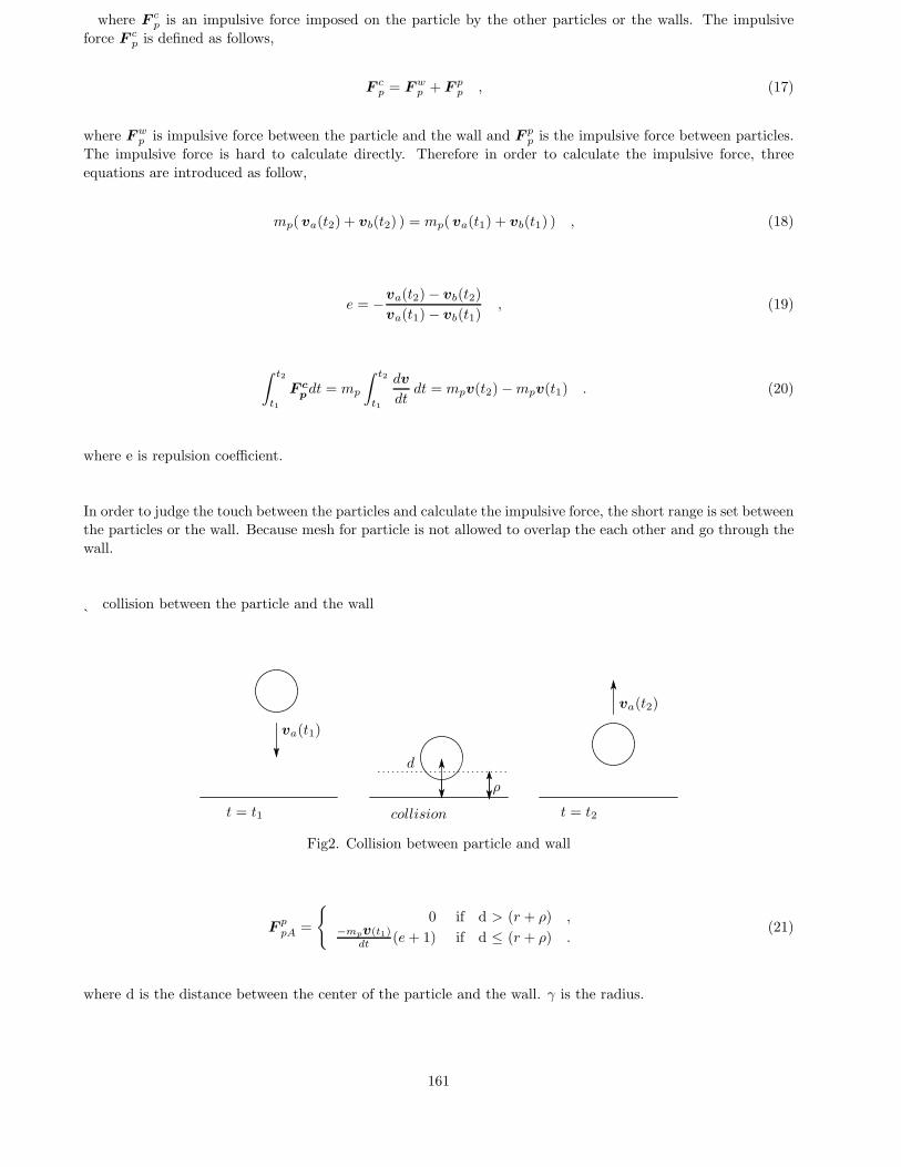
＊ collision between the particle and the wall

va(t1)

va(t2)

ρ

d

t = t1 collision t = t2

Fig2. Collision between particle and wall

F ppA =

0 if d > (r + ρ) ,

−mpv(t1)dt (e+ 1) if d ≤ (r + ρ) .

(21)

where d is the distance between the center of the particle and the wall. γ is the radius.

161

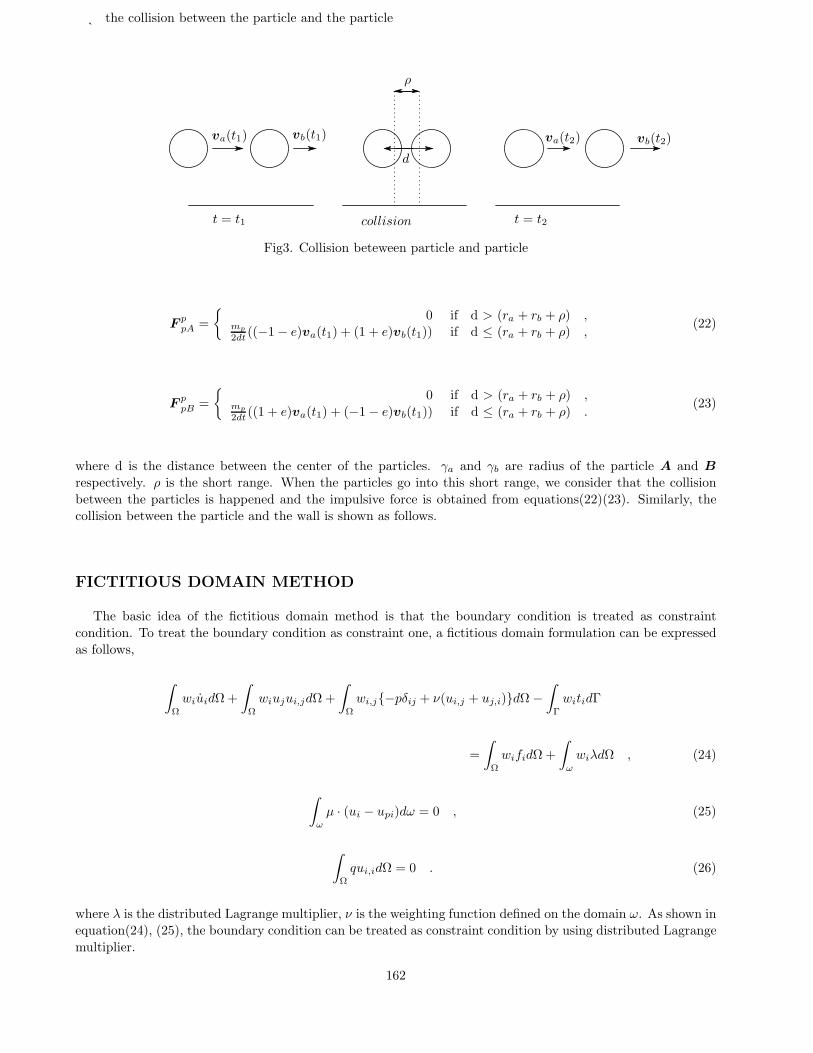
＊ the collision between the particle and the particle

va(t1) va(t2) vb(t2)vb(t1)

ρ

d

t = t1 collision t = t2

Fig3. Collision beteween particle and particle

F ppA =

0 if d > (ra + rb + ρ) ,

mp

2dt ((−1− e)va(t1) + (1 + e)vb(t1)) if d ≤ (ra + rb + ρ) ,(22)

F ppB =

0 if d > (ra + rb + ρ) ,

mp

2dt ((1 + e)va(t1) + (−1− e)vb(t1)) if d ≤ (ra + rb + ρ) .(23)

where d is the distance between the center of the particles. γa and γb are radius of the particle A and B

respectively. ρ is the short range. When the particles go into this short range, we consider that the collisionbetween the particles is happened and the impulsive force is obtained from equations(22)(23). Similarly, thecollision between the particle and the wall is shown as follows.

FICTITIOUS DOMAIN METHOD

The basic idea of the fictitious domain method is that the boundary condition is treated as constraintcondition. To treat the boundary condition as constraint one, a fictitious domain formulation can be expressedas follows,

∫Ω

wiuidΩ+∫

Ω

wiujui,jdΩ +∫

Ω

wi,j−pδij + ν(ui,j + uj,i)dΩ−∫

Γ

witidΓ

=∫

Ω

wifidΩ +∫

ω

wiλdΩ , (24)

∫ω

µ · (ui − upi)dω = 0 , (25)

∫Ω

qui,idΩ = 0 . (26)

where λ is the distributed Lagrange multiplier, ν is the weighting function defined on the domain ω. As shown inequation(24), (25), the boundary condition can be treated as constraint condition by using distributed Lagrangemultiplier.

162

DISCRETIZATION

For the temporal discretization, the Crank-Nicolson method is applied to the momentum equation(24).Pressure, Lagrange multiplier and equation(25) are implicitly expressed. The mixed interpolation is applied tothe spatial discretization. A bubble element adding a bubble function to a bilinear element is employed as aninterpolation for the flow field. A bilinear element is employed as an interpolation for the pressure field.

∫Ω

wiui

n+1 − uin

∆tdΩ+

12∫

Ω

wiujn(ui,j

n+1 + ui,jn)dΩ+ ν[

∫Ω

wi,j(ui,jn+1 − ui,j

n)dΩ

+∫

Ω

wi,j(uj,in+1 − uj,i

n)dΩ] −∫

Ω

wi,iPn+1dΩ−

∫Γ

witidΓ =∫

Ω

wifidΩ+∫

ω

wiλn+1dω , (27)

∫Ω

qui,in+1dΩ = 0 , (28)

∫ω

µhuin+1 − upi

n+1dω = 0 . (29)

In the fictitious domain method, the Dirac’s delta function is applied to the interpolation function of theLagrange multiplier λh and the weighting function µh, which are defined in the domain ω. Where the Dirac’sdelta function is used, it is not necessary to define integral space. Therefore it is possible to integrate on thedomain ω. The approximated Lagrange multiplier µh and the weighting function µh can be written as follows,

λh =Nd∑i=1

λiδ(X −Xi), µh =Nd∑i=1

µiδ(X −Xi). (30)

where Nd is the number of the nodes in the domain ω , δ(・) is the Dirac’s delta function at X=0 defined asfollows,

δ(X −Xi) = ∞ (X = Xi)

0 (X = Xi),(31)

∫ ∞

−∞δ(X −Xi) =

0 (X = Xi)1 (X = Xi).

(32)

Then, the integration on the domain ω can be written as follows,

∫Ω

λhwhdx =Nd∑i=1

λiwh(Xi), (33)

∫ω

µh(uh − up)dx =Nd∑i=1

µi(uh(X)− up(Xi)). (34)

163

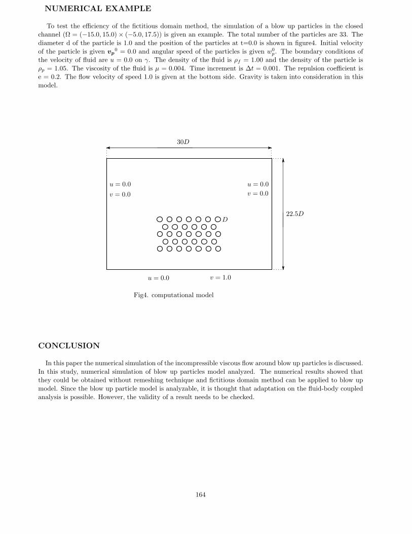
NUMERICAL EXAMPLE

To test the efficiency of the fictitious domain method, the simulation of a blow up particles in the closedchannel (Ω = (−15.0, 15.0)× (−5.0, 17.5)) is given an example. The total number of the particles are 33. Thediameter d of the particle is 1.0 and the position of the particles at t=0.0 is shown in figure4. Initial velocityof the particle is given vp

0 = 0.0 and angular speed of the particles is given w0p. The boundary conditions of

the velocity of fluid are u = 0.0 on γ. The density of the fluid is ρf = 1.00 and the density of the particle isρp = 1.05. The viscosity of the fluid is µ = 0.004. Time increment is ∆t = 0.001. The repulsion coefficient ise = 0.2. The flow velocity of speed 1.0 is given at the bottom side. Gravity is taken into consideration in thismodel.

D

30D

22.5D

u = 0.0v = 0.0

u = 0.0 v = 1.0

u = 0.0v = 0.0

Fig4. computational model

CONCLUSION

In this paper the numerical simulation of the incompressible viscous flow around blow up particles is discussed.In this study, numerical simulation of blow up particles model analyzed. The numerical results showed thatthey could be obtained without remeshing technique and fictitious domain method can be applied to blow upmodel. Since the blow up particle model is analyzable, it is thought that adaptation on the fluid-body coupledanalysis is possible. However, the validity of a result needs to be checked.

164

REFERENCE

1.N.Shimada, ’Fictitious Domain Method based on A Distributed Lagrange Multiplier for Particulate Flows’

2,N.Shimada, ’A Distributed Lagrange Multiplier / Fictitious Domain Method For Incompressible Viscous FlowModeled By Navier-Stokes Equations’

3,Takumi MORIWAKI, ’A Fictitious Domain Method with Distributed Lagrange Multiplier for the NumericalSimulations’

4.keiko KIMURA, ’Incompressible Flows Analysis using Fictitious Domain Method Based on Finite ElementMethod’

5,H.Naya, ’A Fictitious Domain Method for the Incompressible Viscous Flow around a Moving Riged Body’

6,R.Glowinski,T-W.pan and j-periaux, ’A fictitious domain method for Dilichlet problem and applications’,Compute.Methods Appl.Mech.Engrg.,Vol.111,pp.283-303,(1994).

7,R.Glowinski, T.W.pan and j-periaux, ’A fictitious domain method for external incompressible viscous flowmodeled by Navier-Stokes equation’, Comput.Methods Appl. Mech. Eng., 112, 133-148(1994).

165

NUMERICAL RESULT

X

Y

-10 -5 0 5 10 15-5

0

5

10

15

20

X

Y

-10 -5 0 5 10 15-5

0

5

10

15

20

Fig5 t = 0.30 Fig6 t = 3.0

X

Y

-10 -5 0 5 10 15-5

0

5

10

15

20

X

Y

-10 -5 0 5 10 15-5

0

5

10

15

20

Fig7 t = 6.0 Fig8 t = 9.0

X

Y

-10 -5 0 5 10 15-5

0

5

10

15

20

X

Y

-10 -5 0 5 10 15-5

0

5

10

15

20

Fig9 t = 12.0 Fig10 t = 15.0

166

X

Y

-10 -5 0 5 10 15-5

0

5

10

15

20

X

Y

-10 -5 0 5 10 15-5

0

5

10

15

20

Fig11 t = 18.0 Fig12 t = 21.0

X

Y

-10 -5 0 5 10 15-5

0

5

10

15

20

X

Y

-10 -5 0 5 10 15-5

0

5

10

15

20

Fig13 t = 24.0 Fig14 t = 25.0

Fig5.～Fig14. Position of pariticle and velocity of fluid.

167