SLL 79-051/PP

cy 1

L lJCRL-52071

TIME-DEPENDENT PROPAGATION OF HIGH-ENERGY LASER BEAMS THROUGH THE ATMOSPHERE: II

3. A. Fleck, Jr. J. R. Morris M. D. Feit

May 18, 1976 19980309 285 Prepared for U.S. Energy Research & Development Administration under contract No. W-7405-Eng-48

LAWRENCE LIVERMORE LABORATORY University of California/Livermore

PLEASE RETURN TO: DTIC QUALITYINSPECTED 4

-_JD TECHNICAL INFORMATION CENTFR Approved " »FUSTIC MISSILE DEFENSE ORGANIZAfION ApProv^forpub]icre T 7100 DEFENSE PENTAGON

^Ü^onUnJimited | WASHINGTOND.C. 20301-7100 IL HO^f

NOTICE

"This report was prepared as an account of work sponsored by the United States Government. Neither the United States nor the United States Energy Research & Development Administration, nor any of their employees, nor any of their contractors, subcontractors, or their employees, makes any warranty, express or implied, or assumes any legal liability or responsibility for the accuracy, completeness or usefulness of any information, apparatus, product or process disclosed, or represents that its use would not infringe privately-owned rights."

Printed in the United States of America Available from

National Technical Information Service U.S. Department of Commerce 5285 Port Royal Road Springfield, VA 22161 Price: Printed Copy $ ; Microfiche $2.25

Domestic Domestic Page Range Price Page Range

326-350

Price

001-025 $ 3.50 10.00 026-050 4.00 351-375 10.50 051-075 4.50 376-400 10.75 076-100 5.00 401-425 11.00 101-125 5.2,5 426-450 11.75 126-150 5.50 451-475 12.00 151-175 6.00 476-500 12.50 176-200 7.50 501-525 12.75 201-225 7.75 526-550 13.00 226-250 8.00 551-575 13.50 251-275 9.00 576-600 13.75 276-300 9.25 601-up *

301-325 9.75

Add $2.50 for each additional 100 page increment from 601 to 1,000 pages: add $4.50 for each additional 100 page increment over 1,000 pages.

Accession Number: 4029

Publication Date: May 18,1976

Title: Time-Dependent Propagation of High-Energy Laser Beams through the Atmosphere: II

Personal Author: Fleck, JA.; Morris, J.R.; Feit, M.D.

Corporate Author Or Publisher: Lawrence Livermore Laboratory, Livermore, CA 94550 Report Number: UCRL-52071; UC-34 Report Number Assigned by Contract Monitor: SLL 79-051

Comments on Document: Archive, RRI, DEW.

Descriptors, Keywords: Time Dependent Propagation High Energy Laser Beam Atmosphere Movement Stagnation Zone Coplanar Scenario Multipulse Transverse Wind Velocity Hydrodynamic Equation

Pages: 00064

Cataloged Date: Dec 07, 1992

Document Type: HC

Number of Copies In Library: 000001

Record ID: 25515

Source of Document: DEW

\

Distribution Category UC-34

m LAWRENCE LIVERMORE LABORATORY

University of California/Livermore, California/94550

UCRL-52071

TIME-DEPENDENT PROPAGATION OF HIGH-ENERGY LASER BEAMS THROUGH THE ATMOSPHERE: II

J. A. Fleck, Jr. J. R. Morris

■M. D. Feit

MS. date: May 18, 1976

Foreword

This work was done under contract to the U. S. Navy

the Army Missile Command, Huntsville, Alabama, and the

U.S. Energy Research and Development Administration.

-ii-

Contents

Abstract 1

1. Introduction 1

2. Treatment of Moving Stagnation Zones in Coplanar Scenarios ... 9

3. Propagation of Multipulse Laser Beams Through Stagnation Zones 10

4. Effect of Longitudinal Air Motion on Flow in the Neighborhood of a Stagnation Zone for Coplanar Scenarios 16

5. Calculation of Transverse Wind Velocities for Noncoplanar Scenarios 18

6. Steady-State Solutions of Hydrodynamic Equations for Arbitrary Transverse Wind Velocities: cw Steady State .... 20

7. Steady-State Solutions of Hydrodynamic Equations for Arbitrary Transverse Wind Velocities: Multipulse Steady State 22

8. Effect of Noncoplanarity on Propagation of cw Laser Beams Through Stagnation Zones 26

9. Effect of Noncoplanarity of Propagation of Multipulse Beams Through Stagnation Zones 29

10. Single-Pulse Thermal Blooming in the Triangular Pulse Approximation 31

11. Multipulse Thermal Blooming in the Triangular Pulse Approximation 37

Acknowledgment 43

References 44

Appendix A: Adaptive Lens Transformation 45

Appendix B: An Adaptive Algorithm for Selecting the Axial Space Increment 53

Appendix C: Treatment of Multiline Absorption 56

Appendix D: Characterization of Nondiffraction-Limited Beams .... 59

-iii-

TIME-DEPENDENT PROPAGATION OF HIGH-ENERGY LASER BEAMS THROUGH THE ATMOSPHERE: II

Abstract

Various factors that can affect

thermal blooming in stagnation zones

are examined, including stagnation-zone

motion, longitudinal air motion in

the neighborhood of the stagnation

zone, and the effects of scenario

noncoplanarity. Of these effects,

only the last offers any reasonable

hope of reducing the strong thermal

blooming that normally accompanies

stagnation zones; in particular, non-

coplanarity should benefit multi-

pulse more than cw beams. The methods

of treating nonhorizontal winds hydro-

dynamically for cw and multipulse

steady-state sources are discussed.

Pulse "self-blooming" in the triangu-

lar pulse approximation is discussed

in the context of both single and

multipulse propagation. It is shown

that self-blooming and multipulse

blooming cannot be treated independently.

1. Introduction

This is the second report in a

series dealing with the general

problem of time-dependent thermal

blooming of multipulse and cw laser

beams. Time dependence is essential

for describing the propagation of

laser beams through stagnation zones,

which are created whenever the motion

of the laser platform and the slewing

of the laser beam combine to create

a null effective transverse wind

velocity at some location along the

propagation path. The location of

vanishing transverse wind we shall

call the stagnation point, and the

term stagnation zone will refer to

the portion of the propagation path,

extending in both directions from the

stagnation point, where the trans-

verse wind has not yet had time to

blow completely across the beam. The

lack of wind at the stagnation point

creates a steadily decreasing density

and a thermal lens whose strength

grows with time. This report will

continue the study of stagnation

-1-

zones begun in Ref. 1, and discuss

contributions of self-blooming to

multipulse thermal blooming and new

models that have been added to the

Four-D code.

Both pivoted-absorption-cell 2 3

measurements ' and detailed numer-

ical calculations of the experimental 1 4

arrangements ' give evidence that

the blooming effects of stagnation

zones tend to saturate with time.

Thus the beam characteristics seem

to approach a kind of quasi-steady

state, which is possibly a result of

the steady reduction in length of the . , 3 stagnation zone wxth time. Despite

the existence of these quasi-steady

states, calculations for high-power

beams show that stagnation zones can

lead to severe beam degradation.

The notion of a stagnation zone re-

quires that the transverse wind veloc-

ity vanish at at least one position

along the propagation path. There

are always present, however, a number

of additional effects that will pre-

vent a completely stagnant wind con-

dition from occurring at any

position. These effects are:

1. Natural convection

2. Motion of the stagnation point

with time

3. Longitudinal air motion at

the stagnation point

4. Vertical air motion due to

noncoplanar scenario geometry

A realistic appraisal of the influ-

ence of stagnation zones on beam

propagation requires that each of

these effects be assessed and pos-

sibly incorporated into the computa-

tional model.

Natural convection flow at the

stagnation point should be negligible

for practical beam sizes. A 3.8-ym

wavelength and a 474-kW beam power,

for example, give a natural con-

vection velocity of the order of

10 cm/s. For this flow velocity

and a beam radius of 10 cm at the

stagnation point, approximately 2 s

is required for the beam to approach

a steady-state density distribution.

This time is excessive for preventing

or reducing stagnation-zone blooming

effects, which may develop in times

ranging from 1 ms to 0.1 s. At a

10.6-ym wavelength the laser heating

rate of the atmosphere is somewhat

greater for the same intensity, but

the natural convection velocity

scales only with the cube root of the

absorbed power, so flow velocities

would not be significantly above

those for the 3.8-ym case. There-

fore, we shall not consider the

effects of natural convection

further.

Under most conditions the stag-

nation point is not stationary but

moves in the same general direction

as the target with a velocity that

is little different from the

-2-

target's. The parcel of air that

sees a null wind speed changes with

time and thus does not heat up in

the manner of a stationary parcel.

The influence of this stagnation-

point motion on beam propagation was

found to be minimal for a cw wave-

form example treated in Ref. 1.

Stagnation-point motion also turns

out to be unimportant for a multi-

pulse scenario examined in this

report. The conclusion is that

stagnation-point motion is unlikely

to have much, if any, effect in

alleviating stagnation-zone blooming,

since, despite the motion, a sub-

stantial propagation path exists over

which wind velocities are negligible.

The existence of a null transverse

wind-velocity component at a stag-

nation point in no way guarantees a

vanishing magnitude of the wind vec-

tor, because a nonvanishing longi-

tudinal component almost always

exists there. Any air parcel found

within the beam at the stagnation

point will, as a result, exit from

the beam in a finite length of time.

Indeed, in coplanar geometries all

wind-flow trajectories should cross

the beam in two locations: one for

values of z (longitudinal position)

below the stagnation point z , and s the other for values above z . The

s wind flow may be in either the

positive- or negative-3 direction.

In the neighborhood of the stagnation

point, the wind-flow trajectories

will enter one side of the beam,

reverse direction with the beam, and

exit on the same side. The resi-

dence time in the beam for fluid

parcels passing through the beam

center at the stagnation point will,

of course, depend on scenario param-

eters, but for some typical beam

sizes and scenarios this time can be

of the order of 0.5 to 1 s. Longi-

tudinal flow should thus be as

effective as natural convection in

controlling density changes at the

stagnation point. One consequence

of these re-entrant wind-flow

trajectories is that air densities

for z values greater than z could

be influenced hydrodynamically by

densities for z values less than z ; s'

but, for any foreseeable practical

scenarios, the re-entrant times —

except perhaps in the immediate

neighborhood of the stagnation

point — would be considerably longer

than times of interest. Consequen-

tly, hydrodynamic coupling between

points above and below z can be s

safely neglected in cases of prac-

tical interest.

The existence of a position where

the transverse wind velocity vanishes

presupposes the extremely improbable

coplanarity of the laser beam and

the trajectories of its platform and

the target — a situation that is

clearly a limiting case of real-world

-3-

scenarios, which are invariably non-

coplanar. In the more general' case of

noncoplanar geometry, only the wind

component along a certain transverse

axis can be expected to vanish. The

wind vector in the transverse plane

will rotate and attain its minimum

magnitude at the stagnation point.

Since this minimum magnitude can

never vanish, except in a space of

measure zero, a steady state can

always be defined for the governing

hydrodynamic equations. The signif-

icance of this is that, in systems

analysis, steady-state numbers can

always be assigned to stagnation-zone

situations, at least for some nominal

degree of noncoplanarity, and these

numbers can be obtained from simple

and relatively cheap steady-state

calculations. Truly coplanar

stagnation-zone situations, in con-

trast, require time-dependent cal-

culations that are expensive and

require considerable care in

execution.

In the coplanar scenario described

in Ref. 1, for example, if the laser

is given an elevation of 10 m above

the plane containing the target and

the laser platform, the vertical

component of wind velocity at the

stagnation point takes on the value

of 1 m/s. This is sufficient to

establish a steady state in a time

of the order of 0.1 s, which is short

compared to times of interest. The

small vertical velocity component at

the stagnation point leads to sub-

stantial changes in isointensity con-

tours in the focal plane, but the

average intensity is remarkably close

to the quasi-steady-state value

obtained in a time-dependent calcu-

lation for the corresponding coplanar

case.

Thus, small amounts of non-

coplanarity should not be expected

to greatly improve cw laser perfor-

mance in stagnation-zone situations

but should contribute to ease in

understanding and predicting it.

The case of multipulse beams is

another matter. As pulse-repetition

frequencies are lowered, a small

vertical wind component at the stag-

nation point becomes more and more

effective in sweeping out the air

between pulses. The benefits of non-

coplanarity in stagnation-zone

situations should thus be greater for

multipulse beams than for cw beams.

The current status of the Four-D

code is summarized in Table 1, and

recent additions to the code are

described in the body of this report.

We have continued to adhere to the

philosophy that the best way to

approach all laser-propagation cal-

culations is through a single,

unified computer code that can be

applied to any problem. The advantages

of this are threefold. First, it

greatly simplifies bookkeeping (or,

-4-

more appropriately, code-keeping),

since a proliferation of limited

special-purpose codes is avoided.

Second, if each type of calculation

is made a subset of a larger calcu-

lational capability, new features

added to the code — such as data-

processing routines, adaptive-lens

transformations, scenario features,

etc. — are available to all types of

calculation at once. Third, real-

istic simulations are possible, since

a wide range of conditions can be

incorporated into any calculation.

Table 1. Basic outline of current Four-D propagation code.

Variables where x^ y are transverse coordinates and z is axial displacement.

Form of propagation equation Scalar wave equation in parabolic approxi- mation

2ik Z8 dz = vp+ TC(?f -1)8

Method of solving propagation equation

Symmetrized split operator, finite Fourier series, fast Fourier transform (FFT) algorithm

0n+l ( ihz V72\ / ihz 8 = exp (--^ Vj.) exp \- -^ X

e*P | " ~Tv Vj. )g kk

2 2 X = k (n - 1)

Hydrodynamics for steady-state cw problems

Transonic slewing

Uses exact solution to linear hydrodynamic equations. Fourier method for M < 1. Characteristic method for M > 1. Solves

V X dx

9p-, + V -r + pA V. • V. = 0,

y dy ^0 -1 -1

3v, 3t>, if 0\ X dx + V

y ty + viPl o,

i^x h + »y ^T)(PI - Vi) = <? - 1>ar-

Steady-state calculation valid for all Mach numbers except M = 1. Code can be used arbitrarily close to M = 1.

-5-

Table 1 (continued).

Treatment of stagnation-zone problems for cw beams

Time-dependent isobar,ic approximation. Transient succession of steady-state den- sity changes; i.e., solves

Sp-,

TF + v 9P]

dx Y - 1 aJ

Nonsteady treatment of multi- pulse density changes

Changes in density from previous pulses in train are calculated with isobaric approxi- mation using

apn + V

3Pn

3t x dx

_ Y - 1- £ Tln(x,y) 8(t t ) n

Method of calculating density change for individual pulse in train

where Tln(x,y) is nth pulse fluence. Den- sity changes resulting from the same pulse are calculated using acoustic equations and triangular pulse shape.

Takes two-dimensional Fourier transform of

alt .£_

sin 1 -

2e

1 2°e (k

2+k2)1/2t ]

h (k2+k2)1/2tl 2 s\ x y) p

where I is Fourier transform of intensity, and tp is the time duration of each pulse. Source aperture should be softened when using this code provision.

Treatment of steady-state multipulse blooming

Previous pulses in train are assumed to be periodic replications of current pulse. Solves

3P-, + v

X dx

3P, + v

y ty

Treatment of turbulence

Y - 1 J I n

&(t - t ) n

Pulse self-blooming is treated as in the nonsteady-state case.

Uses phase-screen method of Bradley and Brown with Von Karman spectrum. Phase screen determined by

-6-

Table 1 (continued).

Lens transformation and treatment of lens optics

00

r(a?,#) = /

—CO

6k e-x.v(ik ) x r x

0

/. y FV y

a/2 x a(k ,k ) ^"-(k ,k ) , x' y n K x' y '

where a is a complex random variable and $n is spectral density of index fluctuations.

Compensates for a portion of lens phase front with cylindrical Talanov lens trans- formation. Uses in spherical case

Treatment of nondiffraction limited beams

^ + L 'f

where Zf is focal length of lens, z<]> is focal length compensated for by Talanov transformation, and z^ is focal length of initial phase front.

Spherical-aberration phase determined by

,SA 2irA , 2 , 2.2 <J> = —~ (x + y ) ,

or phase-screen method of Hogge et at. Phase determined as in turbulence, only

a2l2 ( lV * = —* exp - -f- n 2TT

where l0 is correlation length and a phase variance.

Adaptive lens transformation Removes phase

2

It ai(xi ~ <**» + h(x<t ~ <\ ^=l

d through lens transformation and deflection of beam. Here xi = x, X2 = y, averages are intensity weighted, oi£ and 3-£ are calcu- lated to keep the intensity centroid at mesh center, and intensity weighted r.m.s. values of x and y are constant with z.

-7-

Table 1 (continued)

Selection of 2-step

Scenario capability

Adaptive s-step selection based on limiting gradients in nonlinear contribution to phase. Constant 2-step over any portion of range also possible.

General noncoplanar scenario geometry capa- bility involving moving laser platform, moving target, and arbitrary wind direction. In coplanar case, wind can be function of t and 3.

Treatment of multiline effects

Calculates average absorption coefficient based on assumption of identical field dis- tributions for all lines

2 — % a =

I

\fi exp(-cus)

fi exp(-ou<0

Treatment of beam jitter

Code output

where fa is fraction of energy in line i at s = 0.

Takes convolution of intensity in target plane with Gaussian distribution:

Vtfr-//■*(- »2 . ,2^ x' + .y'

2a2

x I(x - x\y - yx) da' dy' ,

2 . where a is variance introduced by jitter.

Isointensity, isodensity, isophase, and spectrum contours. Intensity averaged over contours. Plots of intensity, phase, den- sity, spatial spectrum along specific directions, etc., at specific times.

Plots of peak intensity and average inten- sity vs time.

Numerical capacity when used with CDC 7600 and restricted to internal memory (large and small core)

Spatial mesh, 64 x 64, 35 sampling times, no restriction on number of axial space increments.

Problem zoning features Number of space increments in x and y directions must be equal and expressible as a power of 2.

-8-

2. Treatment of Moving Stagnation Zones

in Coplanar Scenarios

The basic coplanar scenario

geometry is depicted in Fig. 1. It

is assumed that the target and laser

platform will collide on the x axis

after a time T has elapsed. The

point of impact is denoted by P and

the position of the laser by L. The

effective transverse wind speed V,

is given by the expression

VV*) = "Sin QT[VT - -§ (Jm - V + V cot 0 J ] R v T p n T

+ vu sin(9„ - ej,(l) w Jw T'

where Vp is the target (receiver)

velocity, 7_ is the laser-platform

(transmitter) velocity, F„ is the

background wind velocity, R is the

Wind vector

Transmitter motion

mpact point

Fig. 1. Diagram of coplanar scenario model.

-9-

range,

vp = vR cos eR , (2)

and

Vn - VR sin 6Ä. (3)

From simple trigonometry,

T co ■-'[

cos ea + <Ve - Z)/Vc

sxn a ]

i? = D sin tj)

sin T

(4a)

(4b)

where 9 is constant.

The transverse wind speed V,

depends on T and hence on time a through the dependence of the

scenario parameters 6_ and R on time

in Eqs. (4a) and (4b). The Four-D

code is programmed to calculate

V,(T .z) as a function of T and V O O

hence of time. The hydrodynamic

equations are solved numerically by

assuming that V. is stepwise constant

over each integration time interval

At.

The location of a stagnation point

is determined by setting the right-

hand side of Eq. (1) equal to zero.

Clearly, that point moves with time,

and, as a result, a different parcel

of air undergoes heating under con-

ditions of zero wind velocity at each

instant. In general the stagnation

point will move with a velocity

comparable to that of the target.

The determination of V, from

Eqs. (l)-(4) for use in the hydro-

dynamic equations permits an accurate

determination of the effect of motion

on the thermal lens in the stagnation

zone. It is more difficult to follow

the irradiance on a moving target,

however, since all equations are

solved in a retarded time frame. It

would be necessary to store the

irradiance history for the values of

s corresponding to the target motion.

Since the relative change of the

range R in a time of interest is

small, it is a good approximation to

assume the focal distance and the

range R at which the laser intensity

is monitored to be constants in time,

while the correct variable R is taken

into account in the hydrodynamic

portion of the calculation by means

of Eqs. (l)-(4).

3. Propagation of Multipulse Laser Beams Through Stagnation Zones

The particular scenario chosen

leads to the effective transverse

wind as a function of range for

T = 0, shown in Fig. 2, where x is

measured from the time the pulse

turns on. The pertinent physical

-10-

data are the following:

Power, P 53 kW

Range, R 2.5 km

Focal length, / 4.5 km

Absorption coefficient, a 0.25 km -1

Wavelength, X

Aperture diameter, 2a 2

(Gaussian at 1/e )

Slewing rate, Q

10.6 um

30 cm

7.44 mrad/s

Pulse-repetition rate, V 10, 25, 50, and 100 s_1

These data can be expressed in

terms of the following dimensionless

numbers:

NF = half = 2.96,

.-2 N = 2a/vQkt = 3.2 x 10 v,

Ns = Üf/VQ =3.6,

NA = af = 1.125,

NDm2 3p

1)E

2 3 a a s (?)

£_ = 100,

where N„3 N 3 N03 N.3 and N-. repre- c O o A U

sent respectively the Fresnel, over-

lap, slewing, absorption, and dis-

tortion numbers. Although the

chosen power, 53 kW, is rather low,

the value of the distortion number

Nn is quite high, and the resulting

thermal blooming is about the maxi-

mum that the code can accommodate.

In any case, the above parameters

>* o o 0) >

c

> c p

Fig. 2.

0.5 1.0 1.5 2.0 2.5 Axial distance — km

Transverse wind velocity as a function of axial distance.

are adequate for assessing the

sensitivity of typical multipulse

laser performance to stagnation-zone

motion.

In the present scenario, the

stagnation zone and target move with

a speed of 300 m/s. For a multi-

pulse beam with V = 100 s , the

stagnation zone moves 3 m between

pulses, whereas for V = 10 s , the

stagnation zone moves 30 m between

pulses. It would be hoped that, in

the case of the lower pulse-

repetition frequency, the greater

movement of the stagnation zone

would lead to a reduced buildup of

stagnant-air density changes. This

effect turns out to be minimal.

The time dependence of the average

intensity on target (averaged over

the minimum half-power area) is

shown for the case of no stagnation-

zone motion in Fig. 3(a) and for the

-11-

ü Vacuum, corrected for linear absorption a Absorbing atmosphere

0.6

Fig. 3. Area-averaged target intensity as a function of pulse time: six pulses at V = 10 s"l. (a) No stagnation-zone motion included, (b) Stagnation-zone motion included.

ft ■.>:■',„')

i!!":'..1';!)!);)

i

!:'. ill

\iwi;_,.v,,1!;: i

?T-=NX

)) ~) ^ \ \

IKiOlW/' '))

i.".:"■■■_■-'. ■-.■■■■■

UlKlK

/feS>

' / / I 1 'l (11 o V) i

1H(K'

Mil

its!)

0.1 0.2 0.3 0.4: 0.5 0.6 s

Fig. 4. Isointensity contours as a function of pulse time for V = 10 s_1.

-12-

Table 2. Comparison of multipulse intensities with and without stagnation- zone motion.

Time-averaged intensity (W/cm ) Time (s)

0.1

0.2

0.3

0.4

0.5

0.6

No motion Average Peak

168.5 234.0

78.9 117.3

60.7 100.7

53.7 92.5

49.6 88.7

47.3 84.1

Motion Average

168.5

78.7

60.8

55.3

52.4

50.2

Peak

234.0

117.3

103.3

96.8

92.7

87.5

Maximum increase resulting from stagnation-zone motion: av, 6.1%; peak, 4.0%.

case with stagnation-zone motion in

Fig. 3(b). The calculation is car-

ried out for six pulses. The isoin-

tensity contours for the six pulses

are shown in Fig. 4 for the moving

stagnation zone. The contours in

the nonmoving case are so similar

that they are not shown. The per-

formance in the two cases is sum-

marized pulse by pulse in Table 2,

where the intensity values have been

averaged over the interpulse

separation time, and the percent

improvements in intensity indicated

are for the last pulse in the train.

Surprisingly, the improvements

in peak and average fluence go in

the opposite direction. The peak

and average fluences are actually

slightly higher in the no-motion

case, as shown in Table 3.

This behavior is due to the large

contribution that the first pulse

in the train makes to the total

fluence. The isofluence contours

for the case with motion are dis-

played in Fig. 5. The central

fluence peak contains the maximum

value and makes the largest contri-

bution to the fluence averaged over

the minimum half-power area.

Apparently in the no-motion case

the subsequent pulses in the train

make a greater contribution in the

central region than do the corre-

sponding pulses in the case with

motion. This small difference in

peak and average fluences is of

Table 3. Comparison of fluences with and without stagnation-zone motion.

Fluence (J/cm2) No motion Motion

Average Peak Average Peak

30.61 42.1 30.1 40.7

Decrease resulting from stagnation- zone motion: av, 1.7%; peak, 3.3%.

-13-

E u I <D 4- o c

o o o

40

30

20

10

>* -10

-20

-30 -

-40

\V^7//!1 i ii, I iii'1' *' i i

7/^\\Y\ if iiüii'.!

i

'Mid!

l -20 -10 0 10 20

x coordinate— cm

Fig. 5. Fluence contours for case of V = 10 s--*-, motion included.

little or no practical importance,

and is indicative of the fact that

stagnation-zone motion plays no

vital role in determining thermal

blooming in stagnation zones.

Figure 6 shows the dependence of

average intensity on time at the

target range for different values

of pulse-repetition rate, V. Each

curve begins with the time of

arrival of the second pulse. (The

first pulse would create a time- 2

averaged intensity of 189 W/cm .)

It is clear that reducing V

diminishes the effect of the stag-

nation zone. The reason obviously

is that for smaller values of V the

air can be swept out by wind between

pulses over a greater proportion of

the propagation path.

Sample pulse-isointensity con-

tours for V = 100 s are displayed

in Fig. 7; these should be compared

with those for V = 10 s in Fig. 4.

At the lower repetition rate, the

beam has divided into two distinct

spots. At the higher rate, lateral

peaks are also formed but they are

much less distinct. The lateral

spreading of the contours as a

function of time is shown in Fig. 8.

The width perpendicular to the wind

0.2 0.4 Time — s

0.6

Fig. 6. Space-averaged intensity as a function of pulse time for various pulse-repetition rates.

-14-

! (i !!''■'O'!!!) I)!

0.01 s

iicnsii II! M

'V /

0.15s

({M ,_ j V

N V 1). ] ■ ' I u |

,i\ i 1

i

!ii

{((& y / // f'J

'/

0.05 s

\

MM! Ill l.'.A1.

/('Ml \ L

NX )

^ .'/>-' V/Mi i. \ I

N^Cw/'Si /

./

0.20 s

HUi) ^/ V \VC~V / / / \\>C1---^/ /

0.10s

III TN V V riss \ i \". ]

Ö i: l ' 'II ill!

Ill/; /- W) k

j

0.25 s

Fig. 7. Isointensity contours for pulses sampled from V = 100 s train.

Fig. 8. Width of beam in direction perpendicular to the wind at various pulse-repetition frequencies.

-15-

is determined by measuring the

maximum distance perpendicular to

the wind direction between 30% con-

tours .

In conclusion, the performance

of a multipulse laser under

stagnation-zone conditions can be

improved by lowering the pulse-

repetition frequency, but, with or

without motion of the stagnation

point, the thermal blooming is

likely to be substantial.

4. Effect of Longitudinal Air Motion on Flow in the Neighborhood of a Stagnation Zone

for Coplanar Scenarios

We wish to examine the air-flow

trajectories in a coordinate system

that moves with the laser beam.

Take the x axis along the direction

of motion of the laser platform and

the y axis perpendicular to it in

the scenario plane. The unit vector

s(t) is directed along the rotating

laser beam, and x1 it) is taken

normal to z(t) (see Fig. 9). At

any instant of time, z(t) and x1it)

can be expressed in the rest frame

of the laser platform by means of

the relations

g(*0 = [cos GyCtO.sin ey(t)], (5a)

£'(t) = [sin Gy(t),-cos er(t)],(5b)

where

JT = cos (£ • x), (6)

and the angle 0„ is calculated from

the scenario Eq. (4a) by substi-

tuting T - t for T . The common

origin for the rest frames of the

laser platform and the rotating

laser beam will be taken at the cen-

ter of the laser aperture.

The effective wind vector in the

moving coordinate system of the

laser can be expressed as

v « = v i —eff -rel Off - V AC*)

X'

x [z(t) £'(*) - x'(t) z(t)]. (7)

Fig. 9. Vector diagram in scenario plane; z(t) indicates instantaneous direction of slewing laser beam.

-16-

Here V„ is the target velocity rela- —TI

tive to the earth's surface, and

^rel = ^ " ^ • (8)

where V^, is the velocity of the

laser platform and V is the veloc-

ity of the wind. An air test par-

ticle will move in the rest frame

of the laser platform along trajec-

tories described by

r(t) = r(0) + V^j* (9)

These trajectories can be expressed

in the rotating frame of the laser

beam by means of the following

relations:

x1(£) = r(t) • £'(*), (10a)

a(t) = r(t) • g(t) . (10b)

Figure 10 shows sample air-

particle trajectories in the vicin-

ity of a stagnation point for four

different scenarios of practical

interest (of the type shown in

Fig. 1). The target range and stag-

nation point location at t = 0 are

indicated in Table 4. At time t = 0

the particles are assumed to be

located precisely at the stagnation

point. The origin of the transverse

coordinate is assumed to be at the

center of the beam. The ticks on

the trajectories indicate points

separated by 0.5 s in time. The

arrows indicate the direction of air

flow with increasing time. Also

shown in Table 4 are the times T

actually spent in the laser beam by

a particle that crosses the stag-

nation point at the center of a

10-cm-radius beam.

The longitudinal wind speed in

the neighborhood of the stagnation

point is roughly equal to V , , as

can be seen from Eq. (7). For the

scenarios described in Table 4,

V , is of the order of 10 m/s. For —rel these scenarios the longitudinal

wind component will be of limited value

in clearing the beam in the vicinity of

the stagnation point.

Table 4. Residence time in beam for air particles passing through stagnation point.

Scenario

Target position at it = 0

(km)

Stagnation at t = (km)

point 0

Res- idence time, T

Cs)

A 1.5 0.844 1.0

B 1.0 0.379 0.5

C 2.5 2.33 1.7

D 1.0 0.295 1.0

-17-

382 rr

6 8 10 0 10

Transverse coordinate (x) — m 30 40

Fig. 10. Air-flow trajectories in rest frame of slewing laser beam in the presence of a stagnation zone. Ticks on the curves denote 0.5-s intervals. (a) Range =1.5 km, stagnation point at z = 0.844 km. (b) Range =1.0 km, stagnation point at z = 0.379 km. (c) Range =2.5 km, stagnation point at z = 2.33 km. (d) Range = 1 km, stagnation point at z - 0.295 km.

5. Calculation of Transverse Wind Velocities for Noncoplanar Scenarios

We shall again assume the

scenario of Fig. 1, only now we

shall relax the»assumption that the

scenario or kinematic plane neces-

sarily coincides with the earth's,

or the horizontal, plane. The line

PLP and the wind vector, however,

will be assumed to lie in the earth's

plane (see Fig. 11). Again, the x

direction will be along the direction

-18-

mpact point

Fig. 11. Diagram of noncoplanar scenario. Laser is now situated at a height h above the platform.

of motion of the laser platform, the

y direction will be in the kinematic

plane, and the unit vector normal

to the kinematic plane will be

called C The laser aperture will

be situated at position L1, which

is at a height h above the line PLP.

The line LL* defines the vector h =

h = hh9 which is normal to the

horizontal plane and makes an

angle 9 with the vector £. The

scenario parameters D3 <J> . R3 8^ l3

and 9~ are now defined in a plane

tilted with respect to the horizontal

plane, but they are related exactly

the same as before. The distance R,

however, no longer has the signifi-

cance of range. The calculation of

the true range i?' is described below.

In order to follow the wind in a

frame of reference that moves with

the laser, it is necessary to intro-

duce an appropriate orthogonal

coordinate system. Clearly this

coordinate system will not be

unique, but a suitable one can be

defined as follows: z is directed

along the laser beam,

y = % x 1T

and

Ä* = $' x §

(11a)

(lib)

It is most convenient to express all

vectors used in the computation in

-19-

the kinematic coordinate system.

Hence we have

vT = (1, 0, 0) ,

VR = (cos 8^, sin 0 , 0),

R = (cos 0y, sin 9^, 0)

h = (0, sin 8 , cos 0 ), p' p' '

Vw = (cos W sxn ör7 cos W P'

(12a)

(12b)

(12c)

(12d)

- sin 0r7 sin 8 ) (12e)

R' R - h (12f)

where V~3 VR3 V^ are unit vectors

directed along V™, V„, and V„, and

the vectors R = RR and R' are directed

along lines extending from L and L',

respectively, to the receiver

(target).

The effective wind seen in the

frame of reference moving with the

laser beam is

W*,*) = % ~ V - w {[^R ~ <V*>»] [Vy - (Vy.g)^]^ (13)

The effective wind components along

X1 and z/' are then obtained from

effar' —eff

V effy' ^eff r (14a)

(14b)

The effective horizontal and ver-

tical wind components in Eqs. (14)

become inputs to the hydrodynamic

calculation which is described in

Sections 6 and 7.

6. Steady-State Solutions of Hydrodynamic Equations for Arbitrary Transverse Wind Velocities:

cw Steady State

Noncoplanar scenarios create

effective winds whose orientation

in the transverse plane vary with

propagation distance z. All

symmetry in the transverse plane

is lost, and the x axis can no

longer serve as the wind axis.

The linearized hydrodynamic

equations must be recast and

solved for a wind having an

arbitrary direction.

The linearized hydrodynamic

equations to be solved are

dP-,

At + P0 1 Zi - 0, (15a)

d v. - -vp, + a. -JL 0 At -1

3y

'■z. dx

'Zv li dx

^ - -I 6. .V dx. 3 "£j

Is

At (?1 ~ °0\) = (Y

-20-

where p.. , v. , and p.. represent the

density, velocity, and pressure per-

turbations induced by laser heating,

n is the viscosity, and the total

derivative -jr is defined by at

d 9 , 9 . 9 f-,r\ -TX = -TTT + v -TT- + v -T-. (16) dt dt x dx y dy

Elimination of p- and V, yields the

following equation for p^

dt\dtT pl"öS

V Pl"3^VplJ

= (Y - 1) av I . (17)

We are interested in the steady state

or the case in which Eq. (17) becomes

i_ + v L x 9cc z/ 3z/ *e V " I ^ v2 ^ - + ^ ^ p, = (Y - l)ari, (18)

where

9P-, 9p1

Pi = v- + V y %y

(19)

The solution for p. is carried out in

two steps: first Eq. (18) is solved

with Pj as dependent variable, and

then Eq. (19) is solved for p1.

We shall restrict our attention to 2 2 the subsonic case, where V + V

2 X V

< G . In that case Eq. (18) is ellip- ö

tic and can be expressed in terms of

a finite Fourier series representation:

P1(aJ»y)

= S P1(VV ^[Ukxx + kyy)] k ,k x* y

(20)

The coefficients p(k.k ) satisfy Xs zr J

\(k ,k ) = - lv x' y' (Y-l)

2 °s J„2 (X + fc )

^<*a»V<*£ + *y>

H „ ' (t; & + v k ) pne2 x x y yJ

lv k + v k V

(21)

where X(fe ,fe ) is the Fourier trans- means of the fast Fourier transform x> y' form of I(x,y). The inverse Fourier (FFT) algorithm. The function

transform of Eq. (21) is evaluated by p.. (x,y) thus obtained then becomes

-21-

3 =

^ =

V A y X

V A X y

V X

the source term for Eq. (19), which If we define

can be solved using the Carlson method

for integration along characteristics.

The solution of Eq. (19) is obtained

by a difference method in configura-

tion space in preference to a Fourier

transform method because the transform

of p^(x,y) will have poles whenever

Vxkx + VyK = °' The evaluation of

the inverse transform by the FFT

algorithm will be troublesome, since

these poles must be avoided.

x'

v JL

(22a)

(22b)

(22c)

the difference equation satisfied

by P-• = P1(iAx,jAy) can be written

PJJ = a" P. ij ß i-i1,3-j ;» + H) ^,j-j'

A. + -JL

2\v p. . + 1,3 3 Pi-i\0-j' + V1 " ßj pi,j-j'J for ß > 1: (23a)

Ptf-ßP*-*',^. + a-0) Pi-i'J

+ rng Yv + 3 pi-'^'+ (1"ß) pi-i',^for 3 <- !■ (23b)

7. Steady-State Solutions of Hydrodynamic Equations for Arbitrary Transverse Wind Velocities:

Multipulse Steady State

Isobaric density changes induced by multipulse heating are governed by

the equation

3p7 + v x dx + V

3pf Y y ty

la 2 y»0*'^ 6(i- v.» (24)

n

where T JM(E,Z/) represents the fluence of the nth pulse, and T represents

-22-

the pulse width. If "steady-state" pulse. Hence I (x,y) = I(x3y) n conditions prevail, it can be assumed Taking the Fourier transform of Eq. (24)

that I does not vary from pulse to with respect to x and y yields

3pf ~, + i{v k + v k )p?p dt xx y y 1

_ T - 1 2

o s °v(vy 26<*-v- (25>

n

Solving Eq. (25) for p p at a time t = mAt, where m is any integer and At

is the time interval between successive pulses, gives

217

pi<WmAlt) = Y - 1 a f(W I expt-i^C^ + y^)]. (26)

n=l

The exponentials in Eq. (26) corres-

pond to translations of the individual-

pulse fluence distributions in con-

figuration space by wind motion.

The summation begins with n = 1

because the isobaric density changes

created by a given pulse do not have

time to develop during the pulse

width, T . The upper limit 217 is

based on numerical considerations and

is determined by

217p = MIN ^inpuf L^rjä*] '

(27)

where 217 is the numerical length of the

mesh used for solving the wave

equation.

-23-

In Eq. (27) MIN signifies the min-

imum of the arguments, and the square

brackets represent the integer part

of the arguments inside them. An

input value of 217 is useful if a true

stagnation point is encountered along

the propagation path. In such cases

the total density change at the stag-

nation point can be kept bounded.

For example, ft. might be set equal

to the actual number of pulses in a

given train, in which case a true

lower bound could be assigned to the

intensities at the target.

The remaining arguments in Eq. (27)

prevent any pulse fluence distribution

from affecting the density calculation

if it has been translated by more

than the minimum (physical) dimension

of the computational mesh for the

wave equation, i.e. MIN(217Aa:J Nhy) .

The density calculation itself is

carried out on a IN x 2N mesh-, which

has a buffer of length N in both the

x and y directions. Thus if Np

satisfies condition (27), periodic

"wrap-around" or positional aliasing

of the density contributions by past

pulses in the train is avoided.

The summation in Eq. (26) may be

luated directly, ar

expressed in the form

evaluated directly, and p can be

wy= - :Lf1 a7( vy exp s

N + 1 "I is-2-^— At(fe v + k v )

a; a; z/

Ü7

sin -^ Ai(fe v ■ + k v ) 2 a: a? .y .y

sin —x- (fey + fe y ) 2 re ic 2/ y

(28)

The density p (a;,z/) is then obtainable

from Eq. (28) by an inverse transform

operation using the FFT algorithm.

Equation (28) has been used in a num-

ber of test examples with satisfactory

results. If the spectrum J(fe .fe ) is ar y'

particularly rich in high spatial fre-

quencies, Eq. (28) may give rise to a

ringing behavior in configuration space

due to the fact that the shift operators

exp (-inktkvj, exp {-inätk v ) (29) XX y y

may not correspond to lattice

translation operators on the compu-

tational mesh. In such a case

ringing can be suppressed by express-

ing the solution of Eq. (26) in

terms of the interpolations of lattice

shift operations.

By means of bilinear interpolation,

one can express any function T(x3y)

at positions intermediate to the lat-

tice by means of

TJ+fx.Wy = (1 - V 4 Vl.fe + (1 " 4> fy Tc,k+1

0 < f < 1 , 0 < f < 1 J x — ' y —

+ Wy W+l+(1- V(1-4)2V,fe> <30>

-24-

where f and / represent fractional may thus be represented in the fol- x y distances between lattice coordinates, lowing alternative form, which avoids

and where the numbers T. , represent the use of nonlattice shift operators

values of T(x3y) sampled at lattice (the notation [ ] signifies the

points. The summation in Eq. (26) integer part of the argument):

N

£ exp [-inM(kxVx + kv )]

n=l

N r V r

- I n=l

4<x /„) expli j -l nk (.[r\xn] + 1) + nv [n„n] y x y * »)

+ fya ~ V exp y £ \\[r]xn] + nk ([V] + 1} >»

+ Vy exp \ £ \\([V]'+ x) + nk ([V] + 1} ■})

TT + (1" V(1"^ eXP ^ {\[V1 + nfe [v]}) r = ^VV' (31)

where

y At

'a; ~ Aa; n„ =

u At ny Az/ »

4(n) = V [V]>

//«> - nyn - [ry,] . >*

(32)

The summation in Eq. (26) over n can

be evaluated as a 227 x 22V DFT with

the aid of the FFT algorithm. For a

given value of n, the numbers [r) n],

[T] n] + 1 can each be identified as

«-coordinates n and the numbers x [ri n] , fr) n] + 1 as y-coordinates n

y u y in the lattice space. Thus each

exponential in the summation in

Eq. (31) can be identified with a par-

As the

index n is incremented, the appro-

ticular lattice point n , n x* y

priate bilinear function of / (n) and tu

-25-

f in) is added to the contents of a a storage register corresponding to

coordinates n , n . On completion of x y this operation, a two-dimensional DFT

of the resultant array will yield the

desired sum (31).

The Fourier transform of the

density can then be expressed as

P±(kx,k mAt) (Y ~ 1) 2 o s

x arc^.y g(kx,ky)

Both the options (28) and (29) are

currently available in the Four-D

code, and the cases run have produced

results that are almost indistinguish-

able.

The shifts and interpolations

implied in Eq. (31) may, of course,

be carried out strictly in configura-

tion space. If N is small, this

procedure may be more economical.

As N becomes large, the Fourier

transform method becomes more

(33) economical.

8. Effect of Noncoplanarity on Propagation of cw Laser Beams Through Stagnation Zones

We shall focus attention on the

scenario discussed in Ref. 1, in

which the total propagation dis-

tance is 1.5 km and the stagnation

point occurs at z = 0.8439 km. The

initial diffraction-limited beam is 2

Gaussian, with 1/g -intensity

diameter of 70 cm, and is assumed

to be focused at the 1.5-km range.

The wavelength and absorption coef-

ficient are assumed to be 3.8 um

and 0.07 km , respectively. For

reference the results of the time

dependent calculations at t = 60 ms

are given in Table 5. For this

value of t, the beam properties are

changing very slowly, and the assump-

tion of a "quasi" steady state is a

reasonable one.

In the noncoplanar scenario, on

the other hand, a true steady state

is known to exist, and a time to

establish this steady state can be

estimated by dividing the beam

diameter by the magnitude of the

vertical wind component at the

stagnation point. The noncoplanar

results are naturally much cheaper

to obtain than the corresponding

coplanar results.

In Table 6, steady-state results

are given for the scenario corres-

ponding to Table 5 for a variety of

elevations of the laser aperture

-26-

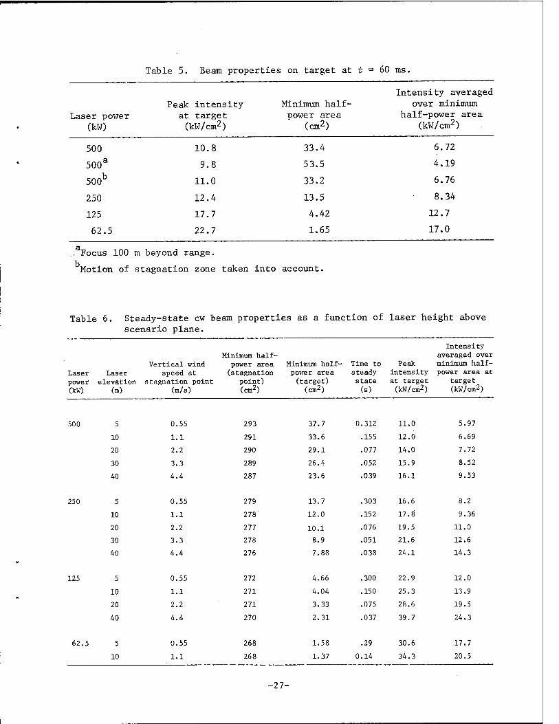
Table 5. Beam properties on target at t - 60 ms.

Laser power (kW)

Peak intensity Minimum half- at target power area

(kW/cm2) (cm2)

Intensity averaged over minimum

half-power area (kW/cm2)

500 10 8 33.4 6.72 * 500a 9. 8 53.5 4.19

500b 11. 0 33.2 6.76

250 12. 4 13.5 8.34

125 17. 7 4.42 12.7

62. 5 22, 7 1.65 17.0

. Focus 100 m beyond range.

Motion of i stagnation zone taken into account.

Table 6 Steady-state cw scenario plane.

beam properties as a funct ion of laser height above

Laser Laser power elevation (kW) (m)

Vertical wind speed at

stagnation point (m/s)

Minimum half- power area Minimum half-

(stagnation power area point) (target) (cm2) (cm2)

Time to steady state

(s)

Intensity averaged over

Peak minimum half- intensity power area at at target target

(kW/cm2) (kW/cm2)

500 5 0.55 293 37.7 0.312 11.0 5.97

10 1.1 291 33.6 .155 12.0 6.69

20 2.2 290 29.1 .077 14.0 7.72

30 3.3 289 26.4 .052 15.9 8.52

40 4.4 287 23.6 .039 16.1 9.53

250 5 0.55 279 13.7 .303 16.6 8.2

10 1.1 278 12.0 .152 17.8 9.36

20 2.2 277 10.1 .076 19.5 11.0

30 3.3 278 8.9 .051 21.6 12.6

V

40 4.4 276 7.88 .038 24.1 14.3

125 5 0.55 272 4.66 .300 22.9 12.0

10 1.1 271 4.04 .150 25.3 13.9

20 2.2 271 3.33 .075 28.6 19.5

40 4.4 270 2.31 .037 39.7 24.3

62.5 5 0.55 268 1.58 .29 30.6 17.7

10 1.1 268 1.37 0.14 34.3 20.5

-27-

0.5 1.0 Axial distance — km

1.5

Fig. 12. Transverse wind velocity as a function of axial distance for cw beam. (a) x com- ponent, (b) y component, (c) Magnitude.

above the scenario plane. Figure 12

shows the variations with z of the

horizontal and vertical components

and the magnitude of the transverse

wind.

From Tables 5 and 6, it is evi-

dent that the space-averaged inten-

sities in the focal plane for the

noncoplanar scenario at 5-m eleva-

tion agree with the corresponding

average steady-state intensities for

Time-dependent coplanar, quasi- steady state

Steady state, noncoplanar, h= 10 m

Fig. 13. Comparison of isointensity contours for stagnation- zone situations in coplanar and noncoplanar cases.

-28-

the coplanar scenarios to within

less than 10%. The peak intensities

for the noncoplanar scenario at 5 m,

on the other hand, are somewhat

higher than the corresponding values

for the coplanar case. There is

also a substantial difference in the

appearance of the isointensity con-

tours in the focal plane (Fig. 13).

As would be expected, performance

improves with height, although the

improvement is marginal for the

elevations considered. In all cases

a steady-state condition can be

reached in a time small compared with

times of interest.

In conclusion, average intensi-

ties for coplanar stagnation-zone

scenarios can be calculated by

adding nominal noncoplanar features

to the scenario and performing a

steady-state calculation. For

cw beams, however, rather

substantial laser elevations

must be provided to alleviate

stagnation-zone effects.

9. Effect of Noncoplanarity of Propagation of Multipulse Beams Through Stagnation Zones

We turn our attention again to

the scenario of Section 3. All

problem parameters are the same,

except that the laser is now assumed

to be elevated 10 m above the

scenario plane. Figure 14 shows the

vertical and horizontal components

of transverse wind velocity as

functions of propagation distance.

Figure 15 shows the isointensity

contours in the target plane for the

various repetition rates.

Table 7 compares laser perfor-

mance on target as a function of

pulse-repetition frequency for the

coplanar scenario and the noncoplanar

scenario with a laser elevation of

10 m. In the absence of complete

steady-state data for the coplanar

case, we have used in Table 7 inten-

sity values corresponding to the

final times exhibited in Fig. 6 for

a given value of V. Thus the

improvements due to noncoplanarity

shown in Table 7 are conservative

estimates.

It is seen from Table 7 that

improvements of at least a factor

of 2, conservatively estimated, are

possible for all values of V. In

the case of V = 10 s~ the laser

performance is even better than it

would be in a vacuum. The reason

is that for this pulse-repetition

frequency the overlap number at the

stagnation point is only 2, and for

-29-

10

5 -

c 0) c o Q_ E o o -5

-10

1 1 1 (a)

1

Stagnation / point —v /

-

'ill 1

Fig. 15. Changing shapes of isoin- tensity contours as a function of pulse-repetition rate for noncoplanar scenario; laser at 10-m elevation.

0.5 1.0 1.5 2.0

Axial distance —km 2.5

Fig. 14. Transverse wind velocity as a function of axial distance for multipulse beam. (a) x component. (b) y component.

overlap numbers in the range 1-2

such enhancement effects for mult

pulse beams are well known.

To summarize: there is clearly

some hope of minimizing stagnation-

zone blooming for multipulse beams

by a combination of elevating the

laser aperture above the scenario

plane and lowering the pulse-

repetition frequency.

-30-

Table 7. Comparison of multipluse beam properties for coplanar and non- coplanar scenarios. Power = 53 kW, range = 2.5 km, A = 10.6 \im, elevation h = 10 m, and vertical wind speed at stagnation point =0.61 m/s.

Intensity Intensity Minimum averaged averaged

half-power Time to Peak over over area steady Overlap Peak intensity minimum minimum

Pulse (stagnation state number at intensity at target half-power half-power repetition point, (non- stagnation at target (non- area area (non-

frequency, noncoplanar coplanar point (non- (coplanar coplanar (coplanar coplanar

V scenario) scenario) coplanar scenario) scenario) scenario) scenario)

(s"1) (cm-2) (s) scenario) (W/cm2) (W/cm2) (W/cm2) (W/cm2)

10 131 0.19 1.9 85.5° 287a 52.0C 181b

25 116 0.18 4.49 59.5C 116 32.5C 65.6

50 104 0.17 8.49 28.7d 70.9 17.8d 42.3

100 140 0.19 19.0 30.4d 49.0 13.2e 30.3

vacuum beam has value 238.

Vacuum beam has value 170. C£ = 0.6 s, steady state has not been reached.

£ = 0.32 s, steady state has not been reached. e-£ = 0.2 s, steady state has not been reached.

10. Single-Pulse Thermal Blooming in the Triangular Pulse Approximation

The isobaric approximation for

changes in air density is invalid

for a single laser pulse whose dura-

tion is comparable to or less than

the transit time of sound across the

beam. In this time regime — referred 3

to as the t -regime because of the

time dependence of density changes

arising from an applied constant

laser-energy absorption rate — the

air-density changes must be deter-

mined from the complete set of time-

dependent hydrodynamic equations,

Eqs. (15).1'7

At late times in the pulse, t

thermal blooming tends to reduce the

on-axis intensity relative to what

it would be if the beam were propa-

gating in vacuum. This reduction

increases with time, and for suf-

ficiently late times a depression

appears in the center of the beam.

Energy added to the pulse at later

times will contribute only margin-

ally to the on-axis fluence. Thus,

for a specific peak pulse

intensity, the on-axis fluence

appears to saturate as the pulse

-31-

duration is stretched out more

and more.

These properties are best illus-

trated by a numerical example. Let

us consider a beam that is Gaussian 2

at z = 0 with I/o -intensity radius

25 cm. The beam, which is focused

at 2.5 km, is assumed to be 2x dif-

fraction limited (A-scaled) with

X = 10.59 ym and a = 0.3 x io~5 cm"1.

The pulse is square-shaped in time

and lasts 100 ys. The choice of a

square-shaped pulse is convenient

because a single calculation con-

tains the complete information for

all square pulses of duration

shorter than the one chosen.

Figure 16 shows the on-axis

intensity at z = 2.0 km, obtained

25 50 75 Time — jus

Fig. 16. On-axis intensity as a function of time. The pulse is taken to be square-shaped in time. Thermal blooming reduces on-axis intensity to a negligible value after a sufficiently long time.

by detailed numerical solution of

Eqs. (15). The on-axis intensity

clearly drops to a negligible value

before the end of the pulse, and,

as a consequence, the on-axis

fluence saturates as the pulse width

increases, as can be seen in Fig. 17.

The detailed temporal evolution of

the spatial shape of the beam is

shown in Figs. 18 and 19. Figure 18

is a three-dimensional plot of the

laser intensity as a function of

time and radius. Figure 19 shows

the radial intensity profiles for

increasing values of time. The

opening up of a hole in the back of

the pulse is clear from both

Figs. 18 and 19.

Calculations of the type repre-

sented in Figs. 17-19 become

impractical if one is treating a

25 50 Time — ^s

75 100

Fig. 17, Saturation of on-axis fluence due to strong pulse thermal blooming.

-32-

CN E o

o o

c (Ü

3 0.

0 10 20 30

Radius — cm

CN E u

c

I I

10 20 30

Radius — cm

Fig. 18. Three-dimensional plot of intensity as a function of time and radius corresponding to Figs. 16 and 17.

Fig. 19. Intensity as a function of radius for increasing time in pulse corresponding to Figs. 16 and 17.

multipulse beam. The determination

of nonisobaric contributions to the

density is greatly simplified by the 1 . triangular pulse approximation, in

which the dependence of the laser

intensity on time is represented as

an isosceles triangle with base

equal to 2T . The density is

required only at time t = T , since

*SP _ PlH = -(Y " 1) OJT

2c 1 -

the laser intensity is assumed to

vanish for t = 0 and t ^ 2x .

The density change at t = T can J p

be evaluated analytically in terms

of a finite Fourier series represen-

tation of the laser intensity. The

Fourier transform of the noniso-

barically induced density change is

-\

(34)

. 2 sin

1/2"

— G x \k + k } 2 s p\ x y 1

where I is the spatial Fourier transform of the intensity. The corresponding

density changes at the grid points are given by the discrete Fourier transform

(DFT) expression

N

pj-wi«.**) - <»r2 I pf (f • f) -p (*&£*) • (35)

-33-

where the basis functions are

periodic on a square of side 2D.

This allows for a buffer region that

extends an additional distance L in

both the x and y directions from the

region of interest.

Comparison of the triangular

pulse approximation and detailed

pulse thermal-blooming calculations

for Gaussian-shaped pulses in time

have shown good agreement between

the calculated fluences for weak or

moderate thermal blooming.

250

CNJ

§ 200

g 150 c CD D

X o c o

100 -

50 -

1 i n

1

7

S3 —

S3 —

/ 1 1 0 25 50 75

Pulse length — ps

100

Fig. 20. On-axis fluence as a function of pulse length, as calcu- lated with triangular pulse approximation (x's) and by detailed numerical solution of hydrodynamic equations for a square pulse in time (solid curve). The tri- angular pulse approximation breaks down as saturated- fluence condition sets in at T = 1.5t . Erratic behavior is due to develop- ment of spikes in the intensity pattern as a function of transverse position.

25 50 75 100

Pulse length — fxs

Fig. 21. Fluence averaged over minimum area containing one half of total beam energy, as a function of pulse length. Solid curve is detailed calculation for square pulse, x's represent triangular pulse approxi- mation.

Figure 20 shows the on-axis fluence

calculated for the previous example

with the triangular pulse approx-

imation (x's) and the detailed

solution of Eqs. (15) for square

pulses in time (solid line).

Despite the difference in assumed

pulse shapes, the agreement between

the two types of calculation is very

good up until time t 52 50 us, which

is well above the saturation time

t = 38 us predicted by the pertur- S 8

bation theory of Ulrich and Hayes 9

based on the work of Aitken et at.

Above 55 Us, or approximately 1.5£ , s

the beam abruptly develops spikes

in its transverse spatial dependence;

-34-

this clearly signals the breakdown

of the triangular pulse approxima-

tion, which must obviously fail when

strong saturation behavior sets in.

Figure 21 shows the fluence

averaged over the minimum half-

energy area (the area within the

one-half peak energy contour) cal-

culated with the triangular pulse

approximation and with the detailed

solution of Eqs. (15) for square

pulses. Both calculations increase

initially, reach a maximum, and then

turn over with increasing time.

This is in part due to the increase

of the area within the one-half peak

energy contour with time. There is,

however, no point in believing the

triangular pulse approximation

beyond the time when the average

fluence curve has reached a maximum,

which also coincides with the onset

of erratic behavior in the on-axis

fluence (Fig. 20).

The perturbation theory alluded

to earlier ' describes the on-axis

fluence saturation for a beam that

is initially Gaussian in shape and

for a pulse shape that is square in

time. In this theory, the expression

for the on-axis intensity is

lit) = «< s '

(36)

where ^n(s) is the on-axis intensity

for a Gaussian beam propagating in

vacuum, or

■T0(0) e

V3) = ~HT)

-as

(37)

Here a is the absorption coefficient

and

D(*) = H)2+(^) . . (38)

where f is the focal distance and a

is the radius of the original

Gaussian beam. The saturation time

t at on-axial position z is given s

by

t = s

2N(y - 1) az2E e aB

3na6D2(z) T

-1/3

(39)

t > t

where N is the refractivity, E is

the pulse energy, and T is the

pulse duration. Since the fluence

cannot be increased for pulses

longer than t , it can be argued s

that nothing is accomplished by

making the pulse longer than t . s The fluence must be maximized

instead by maximizing the product

J (s) t or, equivalently, by u s

maximizing Xn(s). The maximum

allowable value of !()(%) at point z

is normally determined by the con-

dition that it not exceed the break-

down intensity, or

-35-

max JQO) = Ißr) (40)

This maximum allowable intensity in

turn determines a critical input

pulse energy at s = 0 given by

E . = va2t I^D(z)eaZ

crxt s BD (41)

where Eq. (37) has been made use of,

and where t is calculated from s

t = s

2N(y - 1) as J. BD

3a4£(s)

-1/3

(42)

If one is dealing with a multipulse

laser with pulse-repetition fre-

quency V, Eq. (41) can be used to

define a critical input power with

P . = V# .. crxt crxt

= ira vtsIBDP(s)e (43)

The self-consistency of the

triangular pulse approximation, on

the other hand, prevents the on-axis

intensity from ever becoming

negative, but, as previously

remarked, the triangular pulse

approximation breaks down for pulse

energies greater than the value that

maximizes the space-averaged target

fluence. For this pulse energy, the

average and on-axis fluences should

be saturated, and further increases

in pulse energy would give no return.

Figures 22 and 23 have been calcu-

lated with the data on which

1.00

0.75

Jl - b0.50

£15 i c

O 0.25

0 0 0.5 1.0 1.5 2.0 2.5 Normalized input-pulse energy

Fig. 22. On-target fluence from tri- angular pulse approximation averaged over area contain- ing (1 - 1/e) fraction of total beam energy. Range = 1.5 km, J-n-p. = 1.6

106 w/ BD

cm'

0 0.5 1.0 1.5 2.0 2.5 Normalized input - pulse energy

Fig. 23. On-target space-averaged fluence and intensity as functions of input pulse energy for triangular pulse approximation. Range = 2 km, JBD = 3 x 10

6 W/cm2.

-36-

Figs. 16-21 are based, but with the

following differences: the ranges

for Figs. 22 and 23 are 1.5 km and

2.0 km respectively; the values

assigned (somewhat arbitrarily) to 6 , 2

JÜT- at these ranges are 3 x 10 W/cm fi 2

and 1.5 x 10 W/cm .

Both the on-target space-averaged

fluence and intensity (Fig. 23) are

plotted as functions of the input

pulse energy normalized to E .

given in Eq. (42). The space

averaging is over the area contained

within the 1/e energy contour. The

indicated maxima of the average

fluences in both Figs. 22 and 23

occur at an input pulse energy equal

to 1.7Ä . . The space-averaged crit

fluence curves in Figs. 22 and 23

are smoother than those displayed

in Fig. 20 because the former are

averaged over larger areas. The

scaling implications of the pertur-

bation theory described in

Eqs. (36)-(42) are apparently valid

for the triangular pulse approx-

imation, although the maximum useful

pulse energy predicted by the latter

is about 50% greater than that

predicted by the perturbation

theory.

In summary: the triangular pulse

approximation should provide reason-

ably accurate fluence results for

pulse energies up to the values

where strong thermal blooming

saturates the on-axis fluence. The

breakdown of the approximation will

be indicated by the development of

spikes in the transverse spatial

dependence of the beam intensity as

well as by a sharp falloff in the

fluence averaged over some area as

a function of pulse energy.

11. Multipulse Thermal Blooming in the Triangular Pulse Approximation

The propagation of a given pulse

in a train is influenced by both the

nonisobaric density changes

discussed in the previous section

and by the isobaric density changes

due to heating by previous pulses

in the train. But can the self-

blooming and multipulse blooming

effects be treated independently?

If so, the results and discussion

of the previous section suggest

that, as time-averaged laser power

is increased by lengthening the

duration of the constituent pulses

in the train, the time-averaged

intensity on target should saturate

at a value that is predictable from

the saturation fluence for a single

-37-

pulse. If <T> represents the time-

averaged intensity, the maximum

achievable value of <J> for a given

pulse-repetition rate should be

expressible as

<J> = vF ^ , (44) max sat ' v '

where F is the single-pulse Sau

saturation fluence.

In order to test the hypothesis

of the independence of self and

multipulse blooming, a set of cal-

culations has been carried out with

the following set of parameters:

Start beam shape Gaussian, truncated 2

at 1/e radius

Range, R 2.5 km

Focal length/

range, F/R 1.0 and 1.2

Wavelength, X 10.6 ym

Absorption

coefficient, a 0.25 km

Aperture diameter,

2a (Gaussian at

1/e2) 21.2 cm

Wind velocity, y_ 10 m/s

Pulse-repetition

rate, V 33-1/3 and 50 s

Maximum pulse

intensity at

-1

-1

receiver, I 4.9 MW/cm" max

Overlap number,

NQ = 2av/vQ 1.0, 1.5

Figure 24 shows the space-

averaged single-pulse intensity I

for V = 33-1/3 s_1 and NQ = 1, with

F/R = 1.0 and 1.2, calculated as a

function of input time-averaged power

<P> = VEp. The curves have been cal-

culated with and without the effects

of pulse self-blooming. The curve

without self-blooming for F/R =1.2

rises slightly with input power

because of a very slight amount of

pulse overlap. It is clear from

Fig. 24, in any case, that thermal

blooming is due almost entirely to

self-blooming effects. The corres-

ponding curves for space- and time-

averaged target intensities <J> are

displayed in Fig. 25, where

<I> = Jxv (44)

It is seen that <J> with self-blooming

rises initially, reaches a peak, and

then falls. From the analysis of the

previous section, we interpret the

peak values of <I> as the saturated

values.

Figure 26 shows I as a function

of <P> for V = 50 s-1 and NQ = 1.5,

with F/R =1.0 and 1.2. Above <P> =

=0.5 MW, and an enhancement effect

sets in that is greater in the case

of the defocused beam. The corres-

ponding curves for space- and time-

averaged target intensities are shown

in Fig. 27.

A comparison of Figs. 25 and 27

is summarized in Table 8. It is seen

that at V = 50 s~ the power <P> sat

at which saturation of <J> occurs is

-38-

CN E o

I

c

•1 0 •4- V E>8 o

(a) Without self-blooming

With self-blooming

With self-blooming

_L

Without self-blooming

0.5 1.0 1.5

Time-averaged transmitter power - MW

2.0

Fig. 24. Space^averaged intensity on target as a function of time-averaged power at transmitter: V = 33-1/3 s_1, NQ = 1. (a) F/R =1.0. (b) F/R = 1.2.

-39-

CN E u

c

<D

O K-

0) >

(U E

-o c o

0) o a

to

(a)

Without self-blooming

With self-blooming

(b)

Without self-blooming-

With self-blooming

0.5_ 1.0 1.5 Time-averaged transmitter power —MW

2.0

Fig. 25. Space- and time-averaged intensity on target as a function of time- averaged power at transmitter: V = 33-1/3 s-1 Nn = 1. (a) F/R =10 (b) F/R = 1.2. ' °

-40-

(a)

6-

<N E u

h I

.*- "Ü5 c

tJ 0 P> o 8

With self-blooming

Without self-blooming _

With self-blooming

1 0.5 1.0 1.5

Time-averaged transmitter power — MW 2.0

Fig. 26. Space-averaged intensity on target as a function of time-averaged power at transmitter: V = 50 s~l, ^o = 1*5. (a) F/R = 1.0. (b) F/R = 1.2.

-41-

C o I

(U u o a

to

2-

Fig. 27.

Without self-blooming

With self-blooming

0.5 1.0 1

Time-averaged transmitter power —MW 2.0

Space- and time-averaged intensity on target as a function of time- averaged power at transmitter: V = 50 s~l iWi = 1 5 (a) F/R = 1.0. (b) F/R = 1.2.

-42-

Table 8. Saturation of time- and space-averaged target intensity due to self- blooming.

V

(a"1) F/R

<P> sat

(MW)

<J> «- sat (kW/cm2)

33 1/3 1.0 1.0 2.4

33 1/3 1.2 1.2 2.5

50 1.0 1.75 2.7

50 1.2 2.0 3.5

higher for both values of F/R than

it is at V = 33-1/3 s~ . The cor-

responding saturation intensity

values <J> ^ are also greater at -lSat -1

V = 50 s than at V = 33-1/3 s .

If effects of self-blooming are not

included, on the other hand, values

of <J> are always greater at a given

value of <P> in the case of

V = 33-1/3 s"1.

Unfortunately, we have no guide

to the accuracy of the triangular

pulse approximation in the overlap

case as we do in the nonoverlap case.

But the above results strongly sug-

gest that the contributions of iso-

baric and nonisobaric density changes

to thermal blooming of multipulse

beams are interrelated, and that

time-averaged saturation intensities

based on single saturation fluences

may not be applicable for overlap

numbers somewhat above 1. In fact,

overlapping isobaric density patterns

may in certain situations actually

override the effects of single-pulse

nonisobaric density changes.

Acknowledgment

The authors are indebted to C. H.

Woods for the calculations of the ef-

fects of laser elevation on cw laser

performance in Section 9 and for the

effects of pulse thermal blooming on

multipulse propagation in Section 11.

-43-

References

1. J. A. Fleck, Jr., J. R. Morris, and M. Feit, Time-Dependent Propagation

of High Energy Laser Beams Through the Atmosphere, Lawrence Livermore

Laboratory, Rept. UCRL-51826 (1975); UCRL-77719 (1976) to be published

in Applied Physios.

2. R. T. Brown, P. J. Berger, F. G. Gebhardt, and H. C. Smith, Influence

of Dead Zones and Transonic Slewing on Thermal Blooming, United Aircraft

Research Laboratory, East Hartford, Conn., Rept. N921724-7 (1974).

3. P. J. Berger, F. G. Gebhardt, and D. C. Smith, Thermal Blooming Due to

a Stagnation Zone in a Slewed Beam, United Aircraft Research Laboratory,

East Hartford, Conn., Rept. N921724-12 (1974).

4. P. J. Berger, P. B. Ulrich, J. T. Ulrich, and F. G. Gebhardt, "Transient

Thermal Blooming of a Slewed Laser Beam Containing a Regime of Stagnant

Absorber," submitted to Applied Optics.

5. The possibility of such curved flow trajectories in the neighborhood of

the stagnation point was pointed out to one of the authors by B. Hogge,

private communication.

6. J. Wallace and J. R. Lilly, "Thermal Blooming of Repetitively Pulsed

Laser Beams," J. Opt. Soc. Am. 64, 1651 (1974).

7. P. B. Ulrich and J. Wallace, J. Opt. Soc. Am. 63, 8 (1973).

8. P. B. Ulrich and J. N. Hayes, U.S. Naval Research Laboratory,

Washington, D.C., unpublished internal report (1974).

9. A. H. Aitken, J. N. Hayes, and P. B. Ulrich, "Thermal Blooming of Pulsed

Focused Gaussian Laser Beams," Appl. Opt. 1_2, 193 (1973).

_44-

Appendix A: Adaptive Lens Transformation

One key to the successful implementation of a laser-propagation code

is finding a coordinate transformation that keeps the laser beam away from

the calculational mesh boundary and at the same time prevents the beam from

contracting to an unreasonably small fraction of the total mesh area at the

focus. If one is solving the Fresnel equation by the finite Fourier trans-

form method, one may alternatively view the problem in terms of comple-

mentarity: one wishes to find a transformation that simultaneously keeps

the beam intensity small on the mesh boundaries in configuration space and

keeps the Fourier spectrum small on the mesh boundaries in fe-space. If

these two conditions are met, one knows from sampling theory that the

numerical solution is highly accurate.

The Four-D code uses an automated procedure that is designed to keep

the intensity centroid at the center of the mesh and the intensity-weighted

r.m.s. values of x and y constant with propagation distance z. These con-

ditions can be written

!i <Xi>I = °- <Ma>

|j <xi - <xi>)1> = 0 , i = 1, 2 , (Alb)

where

X-. x, Xj y >

/dx dy Iix3ylu

<u>1 = -1 dx dy T(x3y)

(Ale)

/■

Hereafter, all averages will be assumed to be intensity-weighted, and the

subscript I will be dropped.

Conditions (Al) also apply to the adaptive coordinate transformation Al

of Bradley and Hermann, which differs from the one employed in the Four-D

Al. L. C. Bradley and J. Hermann, "Change of Reference Wavefront," Massachusetts Institute of Technology, Lincoln Laboratory, Lexington, Mass., unpublished internal report.

-45-

code only in that it is preceded by a transformation to the coordinates of

an arbitrary Gaussian beam propagating in vacuum. It should be evident, in

any case, that such adaptive transformations are restricted to steady-state

problems, since for time-dependent problems no single transformation will

apply to all time values. To solve time-dependent problems one must employ

a Talanov transformation that is optimized to all time values. This

optimization is accomplished by a combination of trial and error and

intuition.

The splitting algorithm employed in the Four-D code can be written

formally as

g - exp (- w- VjJ exp (- w- x) exp (- J** VJ g^ (A2)

X k2(n2 - 1)

where the middle exponential on the right-hand side of Eq. (A2) contains the

changes in phase resulting from hydrodynamic changes in density, turbulence,

etc. Immediately after this step in the calculation, a quadratic reference

phase front is determined and is removed from 8 by means of a Talanov

transformation and a deflection of the beam coordinates. These operations

are carried out as part of the vacuum propagation step. During vacuum

propagation the solution is advanced by solving

UK. ff = v\g (A3)

Equation (Al) can be written

<xi>

2 <x. > i

= p I dx± dx2 ^1^(^,^2,3)1 ,

= p I &c1 da?2 x±\S{x1,x2,z)\ ,

(A4a)

i = 1, 2 (A4b)

where "P is the beam power given by

P = / dx± dx2 \${x±,x2)| 2

46-

(A5)

By differentiating Eqs. (A4a) and (A4b) with respect to z and making

use of the Fresnel equation (A3), one obtains the following relations:

h<xi>=-WJ ^1 te2\£(xvx2,z)\2 xi^Hxvx2ts)l (A6a)

= - -^p / <&! dx2\s(cc1,x2,z) | -^- <$>(x1,x2,2) , (A6b) •J Is

te<xi>

where the phase cb(a?.. , x^, z) is defined by

4>(.xltx2,z) = Im[lng(x1,x2,z)] . (A6c)

In fc-space one can similarly derive

3 .. T— <X ■> = dz -V

8^2^ 2 _ te<xi >= " W ^

*P JJ dKl dK2 <i\&KvK2>*> \2 =HT- > (A7a)

/ / dKx dK2 K^lJ'^.Kj.a)!

x g^- ip(KrK2,z) , (A7b) i

where «§'(K1 ,K„,<J) is the Fourier transform of &(x^,x~,z) , and

IKK15K2,3) = Im[ln^'(K1,K2,s)] . (A8)

We now wish to determine a phase front that will preserve the following

conditions:

t-<x.> = 0 , (A9a) öz ^

|j<(a? -<xi>)2>= 0 , £=1,2. (A9b)

-47-

Equation (A9b) is equivalent to

WZ<X. > - 2<X.> ir-<X.> = 0. oz ^ % az % (A9c)

From Eqs. (A9) and (A6) one obtains

-Ö— <x •> ds ^ i(w.^ = ° > (AlOa)

7T— <« •> = 02 ?. K** sir V - ° • (AlOb)

Thus the reference phase front must satisfy

dx. i

= 0 (Alia)

<**-<**» -gi-+>- ° • (Al lb)

Let us define a new phase variable:

r (xrx2,zn+li) = V'WW

+ 2 [ai(^ - <xi>)2 + h(xi - <xi>)] > 1.-1

(A12)

where ^Q^l'^'Vf^ rePresents the Phase <Ka1>a?2>JVf}^ at z^ before the

vacuum propagation operator has been applied, and where a,, and ß. are

determined so as to make conditions (Alia) and (Allb) hold for the phase

front ^ {x1,x2,zn^). From Eq, (Alia) we obtain

(■gir^r^'W) = 2ai <*i ~ ^i» + h

(Al 3)

-48-

or

From (Allb) we obtain

(<*i ~ <xi» ir *' <*i> V w) = 2ai({xi - <xi>)2 >

or

a.

\ 9*G

((x. - <^>)2)

+ ß .<rc. - <ic •» = 0

i = 1, 2 (A14)

Equations (A13) and (A14), which determine the desired reference

phase-front parameters (A12), can be shown to be completely equivalent to Al

the relations used by Bradley and Hermann.

If the optimal phase front ((>' is now substituted for the original

phase front <j>0 at zn^, the phase increment

4>0 - *' - S \.*i<*i - <xi»2 + h^i - <xi>)] (A15)

i=l

must be compensated for in some way in order to preserve the original field.

The quadratic contribution in (A15) is compensated for by a generalized

Talanov transformation, which involves a rescaling of <f,the mesh, and As,

according to

£(x,y,z) =

■«('

As1

xl

x Si X Ä2 ' _ As '

x y

z \ exp k I x * Tl s - As

+ s - As

2/ (A16a)

-49-

where

^(lV VS) = ^Kx'Ky*8 " As) exp 2 2

2k (Al6b)

S-, = '1 1 - (As/s )

s^ = 2 1 - (As/a )

(A16c)

(A16d)

The generalized focal lengths z^ and a are determined by combining the

reciprocals of the current focal lengths,

zx = 2a±/k , (A17a)

Zy = 2a2/fe > (A17b)

with those remaining from previous propagation steps (see argument of expo-

nential in Eq, (A16a)).

The linear term in (A15) corresponds to solving Eq. (A3) in a coor-

dinate system that has been rotated in x-y-z space. If this rotation is

assumed to be small, it can be represented by a net deflection in the x and

y coordinates given by

6x = -(ßj/fc)* , (A18a)

Sy = -(ß2/fc)a . (Al8b)

The contribution 2^ ß^(a^ - <a^>) must also be added to <|>0 before the vacuum

propagation calculation, but this operation may correspond to a translation

of the Fourier transform &(<x,Ky) by a nonintegral number of steps on the

-50-

/c-space mesh. In order to avoid this, ß- /AK and 39/AK are both rounded

off to the nearest integer, and &(K 3K ) is then translated on its mesh in x y the x and z/ directions by the corresponding number of steps.

The numerical implementation of Eqs. (A13) and (A14) requires the

following computations, where j and k represent the numerical coordinates

of the mesh points:

3,k

3,k

((x - <x»2) = | £ ^I^'fel2 " * 2 ' (M9)

3>k

I g = «? > ^

2

J K'' \*jk

x V i~ 12

Ä l*7fc'

((* - <x>) H^- (2AZ27)"1

x Im £ ^ (<^ - ^lffc)Mjk + ^_lffe) -<-><|) J,fc

-51-

The computations involving the variable y are carried out in an

analogous manner. In the calculation of the average phase derivative, the

phase derivative is monitored at each point and limited in magnitude to a

fraction of ir. This prevents rapid phase fluctuations near the mesh

boundary, where intensities may be weak, from contributing disproportionately

to the average.

-52-

Appendix B: An Adaptive Algorithm for Selecting the Axial Space Increment

It is desirable to have the code select the next axial space increment

As at a given axial position on the basis of requirements for numerical

accuracy in the solution of the wave equation. The numerical acquracy of

the vacuum propagators in the symmetrically split solution operator,

S = exp (- 4£- Vx 1 exp I- ^- XJ exp I- -^- Vj_. I<?,(B1)

is independent of As if the solution is based on a discrete Fourier trans-

form. The imposition of the phase front,

A* = - |f* , (B2)

at 8 = 3M, which is equivalent to passing the beam through a lens, will

make the solution meaningless if any of the transverse zone-to-zone phase

differences violate

\& (A<j>)| <Jv , (B3)

|S (A(j>)| < /TT , y

0 < f <1 .

It will always be necessary then to restrict the value of As so that con-

ditions (B3) are met. While violating conditions (B3) destroys the numerical

integrity of the solution, satisfying them does not completely guarantee 2

accuracy, sxnce errors can also result from the noncommutation of V_j_ and

X, and from upgrading x to° infrequently. These errors must be controlled

externally by inputting a maximum allowable value of As.

In practice, part of the effect of the phase front (B2) is removed by

the adaptive lens transformation. It would therefore be too restrictive to

limit As on the basis of conditions (B3). As an alternative one can restrict

the value of As so as to control transverse gradients in the phase variable

-53-

0= 1 «i<*i - <*i*/ - ? Jf **\ > CB4)

which is that part of the nonlinear phase front at s ,, that cannot be

removed by the adaptive lens transformation. The next spacial increment W+l n

As is then chosen in terms of the current value As by means of the

relation

A n+1 = __^ fkz\

3k— max

The arguments of the maximum function in the denominator of expression (B5)

are restricted to those mesh points where the intensity is greater than a

certain fraction /' of the maximum intensity. The final value of Asn ,

however, must satisfy the additional constraints:

0.8AsTC < AsW+1 < 1.2 AsW , (B6)

As . < As < As , (B7) mxn — max ' v '

,42f" Az"^1 < —± , (B8)

4^B %rp

k[ ((x - <*»2).+ ((z/ - <y>)2)]

with (B6) taking precedence over (B5), (B7) over (B6), and (B8) over (B7).

In Eq. (B8), / « 0.005 is an input fraction and a_ = min(|s |, \z |).

Condition (B8) is designed to reduce As near a focus, where the geometric-

optics scaling of the mesh by the Talanov transformation may result in an

excessive shrinkage of the mesh. By updating the Talanov transformation

sufficiently often, one can usually avoid a geometric-optics catastrophe.

The adaptive s-step algorithm just described adds greatly to the con-

venience of running problems; it often improves problem running time, and

avoids large nonlinear phase changes that can invalidate the calculation.

It should not, however, be regarded as a panacea. For sufficiently high

beam power and strong enough thermal blooming, the criteria (B5)-(B8) can

-54-

be satisfied and yet the problem still goes bad. In such cases, large non-

quadratic transverse zone-to-zone .phase differences can accumulate over many

s-steps.

-55-

Appendix C: Treatment of Multiline Absorption

The treatment of multiline absorption in the Four-D code follows the Cl

method of Hogge. The basic assumptions are that all lines operate with

the same transverse mode structure in the laser and that the line frequen-

cies are near enough to each other so that the field for each line will be

affected in the same way by the atmospheric density distribution. Thus at

each position g, for the ith line <^.(s) = S{z) , and the field will be com-

pletely characterized by the fractions f.(g) of the total power P(z) that Is

are found in each line.

At g = 0 one has

^(0) = /\(0) P(0) , (cl)

and at position z

P^z) = P^(0) e~alz ,

P(z) = £ P^z) = P(o) £jf\(0) e °^2, (C2)

-a .g fAO) e ^

fA*) = •z- v -a.3" I ^

#0) s

Thus,

Vs) = fiiz) Iiz)> CC31

and the energy-deposition rate per unit volume is given by

Cl. C. B. Hogge, "A Comparison of Several High Energy Laser Systems with Emphasis on Propagation Aspects," in Laser Digest, AFWL-TR-75-140 (May 1975).

-56-

Iw>= J(s) 2<W2) (C4)

in which

I aiVz^ = "^ (C5)

can be interpreted as an average cross section throughout the calculation.

Tables Cl and C2 show values for a(z) as a function of z for the DF

line data found in Ref. C2. Clearly, for DF the effect of including all

line absorption details leads to a very small correction even at 10 km.

Table Cl. Line-by- -line absorption- coefficient data.

Absorption Line frequency Fraction of total power coefficient

Line ID (cm-1) z = 0 z = 10 km (km-1 )

4-3,7 — 0.01040 0.01006 0.06000 3-2,10 2496.77 .00590 .00636 .04920 4-3,6 — .02130 .02060 .06000 3-2,9 2521.81 .01330 .01632 .03620 4-3,5 — .01040 .01006 .06000 3-2,8 2546.42 .04750 .05401 .04380 3-2,7 2570.51 .06380 .06108 .06100 2-1,10 2580.10 .00910 .00813 .06790 3-2,6 2594.25 .08970 .11944 .02800 2-1,9 2605.80 .03180 .03786 .03920 3-2,5 2617.44 .05630 .07960 .02200 2-1,8 2631.06 .08450 .10460 .03530 2-1,7 2655.85 .09040 .05918 .09900 2-1,6 2680.17 .13040 .12864 .05800 1-0,9 2691.61 .03230 .02557 .08000 2-1,5 2703.99 .04000 .05300 .02850 1-0,8 2717.54 .06440 .03629 .11400 1-0,7 2743.00 .08740 .08434 .06020 1-0,6 2767.97 .08370 .06178 .08700 1-0,5 2792.43 0.02740 0.02310 0.07370

C2. R. K. Long, F. S. Mills, and G. L. Trusty, Calculated Absorption Coefficients for DF Laser Frequencies, Ohio State University Electro- Science Laboratory, Rept. RADC-TR-73-389.

-57-

Table C2. Mean absorption coefficient as a function of distance.

Propagation distance

(km)

0 1 2 3 4 5 6 7 8 9

10

Mean absorption

coefficient (km-1)

0.06001 0.05931 0.05862 0.05793 0.05726 0.05660 0.05594 0.05530 0.05467 0.05404 0.05343

Remaining power

fraction in beam

1.00000 0.94209 0.88815 0.83787 0.79097 0.74720 0.70632 0.66811 0.63236 0.59891 0.56758

-58-

Appendix D: Characterization of Nondiffraction-Limited Beams

In the absence of detailed a priori information regarding the exact mode

content of a beam, several models of nondiffraction-limited beam behavior can

be applied with the Four-D code.

The simplest of these, which requires no special coding, is wavelength

scaling, wherein the laser wavelength is multiplied by a number equal to the

beam quality factor. Wavelength scaling gives the correct vacuum peak

intensity, although it may incorrectly represent the vacuum focal-spot size.

It represents, in any case, a prescription whose accuracy needs to be evaluated

ad hoc for each specific application. While it has been useful in a variety

of applications, it does not properly account for discrepancies between cal-

culations and stagnation .blooming experiments in vertical absorption cells.

Agreement between measured data and calculations for these experiments

is improved, on the other hand, by adding spherical aberration to the initial

beam in such a way that the vacuum focal-spot size is correctly reproduced

(see Fig. Dl). The spherical aberration contribution to the initial phase can

be represented as

,SA 2TL4 , 2 _, 2N2 <i> = —2 ^x y'

a x

(Dl)

where A represents the number of waves of aberration at radius 0 . X D2 A third model of nondiffraction-limited behavior is due to Hogge et at.

This model is based on the assumption that the initial beam can be represented

80e,y.,0) = gQ(x,y) e^(x*y) , (D2)

where the phase aberration§(x,y) is a Gaussian random variable, arising from

laser-medium inhomogeneities, mirror imperfections, etc. If it is assumed

that the correlation function for phase fluctuations is

Dl. J. A. Fleck, Jr;, J. R. Morris, and M. D. Feit, Time-Dependent Propagation of High Energy Laser Beams Through the Atmosphere, Lawrence Livermore Laboratory, Rept. UCRL-51826 (1975).

D2. C. B. Hogge, R. R. Butts, and M. Burlakoff, Appl. Opt. 13, 1065 (1974)

-59-

C.(r) = a. exp . 21

(D3)

0,

2 2 2 2 where r = x + y , a^ is the variance of <j>, and Z.Q is the phase coherence

length, then the spectrum of the phase fluctuations is given by

<j> -^ 2TT exp I-

I1 klS

(D4)

l.Ot

^ 0.6 c

>

cS 0.4

-" — —— Unbloomed

■■ Calculated

——- — Calculated with A/25 spherical aberration

Experiment

0 =0.178 rad/s

x = 0.48

.0.06 0.08 0.10 Time — s

Fig. Dl. Intensity on target after passing through stagnation zone. Com- parison between experiment and calculation with and without spherical aberration. (Data from P. J. Berger, F. G. Gebhardt, and D. Smith, Thermal Blooming Due to a Stagnation Zone in a Slewed Beam, United Aircraft Research Laboratory, East Hartford, Conn., Rept. N921724-12 (1974).)

-60-

Using the method of phase screens, one can obtain the Fourier transform of

the phase §(x3y) to be used in Eq. (Dl) in the following form:

/a'(k.) + ia"(k.)\ ^ (D5)

where a' and a" are Gaussian random variables with variance 1, and where

a'O^) = a'C-k^) ,

a»^) - -a"(-k^)

(D6)

Equations (D5) and (D6) were originally included in the Four-D code for

simulating turbulence, The phase-screen model of nondiffraction-limited

beams utilizes the same subroutines.

The following parameters were the basis of an example for comparing the

difference between the wavelength-scaling and the phase-screen models of non-

diffraction-limited behavior:

Beam shape

Aperture size, 2a

Range

Absorption coefficient, a

Transverse wind speed, V

Focal distance, /

Beam is 2* diffraction limited

Wavelength, X

Scaled wavelength, X

Phase correlation length, I

Phase standard deviation, 0,

Number of phase-screen calculations

for ensemble average 10

Gaussian

80 cm

2.5 km

0.07 km"1

10 m/s

2.5 km

5.7 ym

11.4 urn

5.0 cm

1.177 (rad)

-61-

Table Dl gives a comparison of peak intensities in the focal plane for propa-

gation in vacuum and air. Also included are results for a uniformly illumina-

ted aperture of radius aQ = 2a, which can likewise be used as a model of a 2x

diffraction-limited beam.

Table Dl. Comparison of peak intensities in the focal plane. Beam propagates in vacuum (linear) and air (nonlinear). Case: Gaussian diffraction- limited beam, a uniformly illuminated aperture (top hat), Gaussian wavelength scaled (2x diffraction limited), and a Gaussian beam with a phase screen adjusted to 2x diffraction limited.

Peak intensity in Model focal plane (kW/cm2)

Linear

Gaussian, A 63.8

Gaussian, 2A 15.9

Top hat 17_4

Phase screen 17.7

Nonlinear

Gaussian, 2A 5.94

Top hat 5#47

Phase screen 3.03

The nondiffraction-limited beams all give roughly one quarter of the

focal-plane intensity of the diffraction-limited beam when propagated in

vacuum. For propagation in a real absorbing atmosphere both the scaled wave-

length and the top-hat beam calculations result in twice the peak intensity

of the phase-screen model calculation, which is based on an ensemble average

taken over 10 independent phase screens. Figures D2 and D3 show respectively

the beam intensity as a function of position along the a;-axis and along a line

parallel to the y-axls passing through the point of maximum intensity along the

ar-axis for the wavelength-scaled beam. Figures D4 and D5 show the same plots

-62-

I4 1 3

4-

C 2.2 c

1 i i r

J L -10

i—i—i—i—f-

J_J I L

10

Fig. D2. Wavelength scaling for 2x diffraction-limited beam. Intensity on target as a function of s along x-axis.

CM E u

c

Fig. D4. Phase-screen model of 2x diffraction-limited beam averaged over 10 independ- ent realizations. Inten- sity on target as a function of x along 37-axis.

Fig. D3. Wavelength scaling for 2x diffraction-limited beam. Intensity on target as a function of y along a line parallel to ?/-axis and passing through point of maximum intensity along the a;-axis.

for the ensemble averaged phase-

screen calculation. In the case of

the wavelength-scaled calculation,

thermal blooming leads primarily to

a broadening of the beam. In the

phase-screen calculation, thermal

blooming is accompanied by con-

siderable scattering of energy to the

far reaches of the mesh.

From these calculations it can

be concluded that different models

of nondiffraction-limited beam

behavior can lead to qualitatively

as well as quantitatively different

thermal-blooming behavior. Which

-63-

-20 -10

y — cm

model is best must be determined for

each specific situation. In the last

analysis there is no substitute for an

accurate experimental characterization

of the beam for each specific laser.

Fig. D5. Phase-screen model of 2x diffraction-limited beam averaged over 10 independ- ent realizations. Inten- sity on target as a function of y along a line parallel to y-$xls and passing through point of maximum intensity along the x-axis.

GS/11/mm/edas/la

-64-