A fully coupled 3-D ice-sheet–sea-level model: algorithm and

Geosci. Model Dev., 7, 2141–2156, 2014www.geosci-model-dev.net/7/2141/2014/doi:10.5194/gmd-7-2141-2014© Author(s) 2014. CC Attribution 3.0 License.

A fully coupled 3-D ice-sheet–sea-level model:algorithm and applications

B. de Boer1,2,*, P. Stocchi3, and R. S. W. van de Wal2

1Department of Earth Sciences, Faculty of Geosciences, Utrecht University, Utrecht, the Netherlands2Institute for Marine and Atmospheric research Utrecht, Utrecht University, Utrecht, the Netherlands3NIOZ, Royal Netherlands Institute for Sea Research, Den Burg, Texel, the Netherlands

* Invited contribution by B. de Boer, recipient of the EGU Outstanding Student Poster Award 2013.

Correspondence to:B. de Boer ([email protected]) and P. Stocchi ([email protected])

Received: 7 May 2014 – Published in Geosci. Model Dev. Discuss.: 23 May 2014Revised: 19 August 2014 – Accepted: 24 August 2014 – Published: 23 September 2014

Abstract. Relative sea-level variations during the late Pleis-tocene can only be reconstructed with the knowledge of ice-sheet history. On the other hand, the knowledge of regionaland global relative sea-level variations is necessary to learnabout the changes in ice volume. Overcoming this prob-lem of circularity demands a fully coupled system where icesheets and sea level vary consistently in space and time anddynamically affect each other. Here we present results forthe past 410 000 years (410 kyr) from the coupling of a setof 3-D ice-sheet-shelf models to a global sea-level model,which is based on the solution of the gravitationally self-consistent sea-level equation. The sea-level model incorpo-rates the glacial isostatic adjustment feedbacks for a Maxwellviscoelastic and rotating Earth model with coastal migra-tion. Ice volume is computed with four 3-D ice-sheet-shelfmodels for North America, Eurasia, Greenland and Antarc-tica. Using an inverse approach, ice volume and temperatureare derived from a benthicδ18O stacked record. The derivedsurface-air temperature anomaly is added to the present-dayclimatology to simulate glacial–interglacial changes in tem-perature and hence ice volume. The ice-sheet thickness vari-ations are then forwarded to the sea-level model to computethe bedrock deformation, the change in sea-surface heightand thus the relative sea-level change. The latter is then for-warded to the ice-sheet models. To quantify the impact of rel-ative sea-level variations on ice-volume evolution, we haveperformed coupled and uncoupled simulations. The largestdifferences of ice-sheet thickness change occur at the edgesof the ice sheets, where relative sea-level change significantlydeparts from the ocean-averaged sea-level variations.

1 Introduction

Periodical expansion and retreat of continental ice sheets hasbeen the main driver of global sea-level fluctuations duringthe Pleistocene (Fairbridge, 1961). Similarly, deep-sea ben-thic δ18O records, a proxy for deep-water temperature andice volume, indicate that the volume of the oceans oscil-lated throughout the Pleistocene in response to global cli-mate changes (Chappell and Shackleton, 1986; Lisiecki andRaymo, 2005). The separation of the benthicδ18O signal intodeep-water temperature and ice volume can be deduced byusing a combination of ice-sheet models and an air-to-oceantemperature coupling function (de Boer et al., 2013). How-ever, the exact contribution of the different ice sheets to thespatially varying relative sea level (RSL), i.e. the change ofthe sea surface relative to the solid Earth, is unknown.

One of the best studied intervals in the past is the lastglacial maximum (LGM,∼21.0 kyr ago), for which a wealthof observational data has been collected, for example RSLand extent of the ice sheet. The LGM was a glacial eventduring which continental ice sheets covered large portionsof North America and Eurasia, and when the ice sheets onAntarctica and Greenland extended towards the continentalshelf edge (e.g.Ehlers and Gibbard, 2007; Denton et al.,2010). Several well-dated surface geological features of de-positional and/or erosive origin constrain the maximum ex-tent of these LGM ice sheets (Ehlers and Gibbard, 2007).The estimated total volume of ice inferred from the RSL datacorrelates well with the ice-sheet volume increase inferredfrom the benthicδ18O data (Lisiecki and Raymo, 2005). Both

Published by Copernicus Publications on behalf of the European Geosciences Union.

2142 B. de Boer et al.: Global coupled 3-D ice-sheet–sea-level model

benthicδ18O records and surface glacial geological featuresshow the−120 to−130 m relative sea-level low stand thatwas recorded by submerged fossil coral terraces at Barba-dos (Peltier and Fairbanks, 2006; Austermann et al., 2013),Tahiti (Bard et al., 1996, 2010; Deschamps et al., 2012) andBonaparte Gulf (Yokoyama et al., 2000). The sea-level riserecorded at these far-field sites during the last∼ 19 kyr fol-lowing the melting of the LGM ice sheets is consistent witha decrease of benthicδ18O. This marks the transition to thecurrent warmer interglacial (Fairbridge, 1961).

However, several coeval post LGM paleo-sea-level indica-tors from different regions are found at present at very dif-ferent elevations above and below the current mean sea level(Pirazzoli, 1991). In particular, a long-term sea-level fall isobserved in the proximity of the former LGM ice sheets(Lambeck et al., 1990). Moving slightly away from the for-merly glaciated areas, the sea-level trend first switches to-wards a steep rise (Engelhart et al., 2011), reaching a mid-Holocene high stand (Basset et al., 2005) and then smoothlychanges towards a eustatic-like sea-level fall that is observedat the far-field sites like Barbados and Tahiti (Fairbanks,1989; Peltier and Fairbanks, 2006; Bard et al., 1996, 2010;Deschamps et al., 2012). This illustrates that the regionallyvarying sea-level changes resulting from the melting of theLGM ice sheets shows that the spatial variability of sea-levelchange strongly depends on the distance from the former icesheets and also on the shape of the ocean basins (Pirazzoli,1991; Milne and Mitrovica, 2008).

Following the deglaciation of an ice sheet, the solid Earthrebounds upwards beneath the former glaciated area, whilethe far-field ocean basins experience subsidence as a conse-quence of the increasing ocean water loading. Therefore, ifthe ice-sheet thickness variation is the forcing function forthe sea-level change, the solid Earth response plays an im-portant role as a modulator of sea-level change. Global sea-level changes during the Holocene and in particular the last6000 years (Pirazzoli, 1991) show that the solid Earth con-tinued to deform after the North American ice sheet (NaIS)and the Eurasian ice sheet (EuIS) were completely melted.This delayed response implies that the solid Earth behaveslike a highly viscous fluid on geological timescales (Ranalli,1985; Turcotte and Schubert, 2002). Additionally, the currentvertical land uplift shown by GPS observations over the for-merly glaciated areas of Scandinavia and Hudson Bay alsoimplies that the solid Earth is not in isostatic equilibrium(Milne et al., 2001).

The mean sea surface is also affected by the gravitationalpull exerted by the continental ice sheets on the ocean wa-ter. During the melting of an ice sheet, the ocean volumeand thus the hypothetical eustatic sea level, i.e. the globalmean change in sea level, are increasing. However, due tothe smaller ice mass there is a reduction in the gravitationalpull exerted on the ocean water, which causes a sea-level fallat the ice-sheet margins and a rise, more than it would do eu-statically, far away from the ice sheet. This effect is known

as self-gravitation (Woodward, 1888), and combined withthe solid Earth deformation it attributes a large proportionof the spatial variability of the sea-level change (Farrell andClark, 1976). Furthermore, due to the rotation of the Eartharound its axis, any surface mass displacement together withthe solid Earth and geoidal deformations triggers a perturba-tion of the polar motion that in turn affects the redistributionof melt water in the oceans and ,hence, the mean sea-surfaceheight (Milne and Mitrovica, 1996; Kendall et al., 2005).

All the feedbacks described above make up the complexprocess known as glacial-hydro isostatic adjustment (GIA),which includes deformation of the Earth and changes of thegeoid, and describe any sea-level change that is dictated byice-sheet fluctuations (Farrell and Clark, 1976). According tothe GIA theory, the sea-level change recorded at any locationrepresents the combined response of the solid Earth and ofthe geoid to the ice-sheet fluctuations; it cannot be directlyused as representative of the eustatic sea-level change. GIAfeedbacks produce mutual motion of the solid Earth and ofthe geoid, and hence any land-based sea-level indicator is es-sentially a RSL indicator as it records the local variation inthe vertical distance between the geoid and the bottom of theocean.

The GIA feedbacks are usually accounted for by solvingthe gravitationally self-consistent sea-level equation (SLE),which was initially developed byFarrell and Clark(1976),and subsequently updated to include all the GIA feedbacks(Mitrovica and Peltier, 1991). The SLE describes the globalRSL change for a prescribed ice-sheet chronology and solidEarth rheological model (Spada and Stocchi, 2007). The SLEhas been widely employed to improve and refine our knowl-edge of the LGM ice-sheet’s volume, thickness and extentand their subsequent deglaciation until the present day (e.g.Peltier, 2004; Spada and Stocchi, 2007; Whitehouse et al.,2012a; Stocchi et al., 2013; Gomez et al., 2013).

To explain the observed RSL changes over the past glacialcycles, a global ice-sheet model is needed to calibrate thecorresponding ice volume. At the same time, the observedRSL changes are needed to verify the simulated ice volumewith the global ice-sheet models. This problem of circularityfollows from the fact that the evolution of the ice sheets iscoupled to the RSL changes. Most importantly the ice-sheet-induced RSL changes affect the growth and retreat of marineice sheets, which are in direct contact with the ocean. Forexample, due to the self-gravitational pull of the ice sheet, theRSL close to the ice sheets actually rises when an ice sheetgrows, this will then counteract the advance of the (marine)ice sheet into the ocean.

Thus far most transient simulations of ice sheets have beencarried out using a global average sea level (Huybrechts,2002; Zweck and Huybrechts, 2005; Bintanja and Van deWal, 2008; Pollard and DeConto, 2009, 2012; de Boer et al.,2013). There have been no studies that simulate a mutu-ally consistent solution of ice volume and regional sea levelthat include multiple ice-sheet models over longer timescales

Geosci. Model Dev., 7, 2141–2156, 2014 www.geosci-model-dev.net/7/2141/2014/

B. de Boer et al.: Global coupled 3-D ice-sheet–sea-level model 2143

(Clark et al., 2002; Weber et al., 2011; Raymo and Mitrovica,2012). During the mid-1970s the importance of including theeffect of relative sea-level change on the instability of ma-rine terminating ice sheet was recognised (Weertman, 1974;Farrell and Clark, 1976). This is important because sea-levelchange has a strong influence on the dynamical behaviour ofmarine ice sheets (e.g.Gomez et al., 2010a, 2013) such as theWest Antarctic ice sheet (Pollard and DeConto, 2009). Onlyrecently,Gomez et al.(2013) have succeeded in coupling asingle 3-D ice sheet with a sea-level model for simulating theAntarctic ice sheet from the LGM to the present. Henceforth,it is of vital importance to incorporate regional sea-level vari-ations when modelling ice sheets over 103–106 years.

In this paper, we present a system of four regional 3-Dice-sheet-shelf models (de Boer et al., 2013) that is fully dy-namically coupled to a global GIA model based on the SLE.WhereGomez et al.(2013) employed a similar system forthe Antarctic ice sheet, our algorithm represents a method formodelling ice-sheet fluctuations and the related GIA-inducedrelative sea-level changes on a global scale. In addition, itis dynamically coupled to a deformable Earth model wherecrustal and geoidal deformations account for self-gravitation,Earth rotation and an adequate treatment of the migration ofcoastlines. Our new model offers the opportunity to modelany ice-sheet and sea-level fluctuation, from the past to thepresent day as well as into the future. Here, we include atemporal discretisation of past ice-sheet fluctuations with amoving time window that allows us to calculate RSL as afunction of the total ice-sheet volume change over the globeover four glacial cycles, starting 410 kyr ago. This allows acomparison with any local record of RSL during this period.

2 Methods

In this study we present a new system that is based on the dy-namical coupling between (i) ANICE, a fully coupled systemof four 3-D regional ice-sheet-shelf models (de Boer et al.,2013) and (ii) SELEN, a global scale SLE model that ac-counts for all the GIA feedbacks (Spada and Stocchi, 2007).In the following, we first describe separately the ANICE andSELEN sub-systems and subsequently introduce the cou-pling method/algorithm with particular emphasis on spatial(see Appendix A) and temporal discretisation.

2.1 The ANICE regional ice-sheet-shelf model

ANICE is a 3-D coupled ice-sheet-shelf model (Bintanja andVan de Wal, 2008; de Boer et al., 2013, 2014). It is a shallow-ice model, for which we use approximate equations for sheetand shelf flow. These approximations are based on the shal-lowness of a large ice body, with horizontal scales far largerthan the thickness of the ice. In ANICE, we apply two ap-proximations, the shallow-ice approximation (SIA) (Hutter,1983) that is used as the basis for land based ice flow, and

Table 1.Separate model parameters for the four ice-sheet models.

Parameter Description EuIS NaIS GrIS AIS

nx ANICE x grid points 171 181 141 141ny ANICE y grid points 105 121 77 1411x grid scale (km) 40 40 20 40Eice SELEN elements 8766 7549 750 8947

the shallow-shelf approximation (SSA) (Morland, 1987) thatis used for floating ice and sliding velocities (de Boer et al.,2013). The latter is computed for both grounded and floatingice; thus, incorporating the transition zone from sheet to shelf(Winkelmann et al., 2011; de Boer et al., 2013).

Within this framework we incorporate four separate ice-sheet models for the regions with major ice sheets during thePleistocene: the Antarctic ice sheet (AIS), the Greenland icesheet (GrIS), the NaIS and the EuIS. The models are solvedseparately on a rectangularx–y grid (see Table1). Ice tem-peratures and velocities are solved in three dimensions with15 grid points in the vertical, which are scaled with ice thick-ness and have a higher resolution at the bottom, starting with1 % and increasing to 10 % at the top.

We adopt the initial basal and surface topographies forAntarctica from the ALBMAP data set (Le Brocq et al.,2010) and for Greenland fromBamber et al.(2001). Theinitial topography for Eurasia and North America is basedon a high-resolution present-day (PD) topography data set(SRTM30_PLUS;Becker et al., 2009). For the initial cli-mate forcing, we use the PD meteorological conditions fromthe ERA-40 Re-analysis data set (Uppala et al.,2005). Wecalculate monthly averages from 1971 to 2000 for precipita-tion (in m w.e. yr−1), 2 m surface-air temperature (◦C), and850 hPa wind fields (in m s−1). The surface topography forthe EuIS and NaIS and the ERA-40 climate fields are in-terpolated on the rectangular ANICE grids with an obliquestereographic projection using the OBLIMAP programme(Reerink et al., 2010). The AIS, EuIS and NaIS models in-corporate grounded and floating ice and a sub-shelf meltingparameterisation, whereas for the GrIS we only consider iceon land (de Boer et al., 2013). All four models are solved withtheir own internal time step varying between 1 and 5 years,depending on the stability criterion, i.e. the ice velocity can-not exceed the grid scale (Table1) divided by the time step.

The uncoupled ice-sheet model ANICE accounts for theregional bedrock deformation that is calculated from varia-tions in ice thickness and ocean water by means of a twolayer flexural Earth model, a flat elastic lithosphere (EL)resting over a viscous relaxed asthenosphere (RA), i.e. theELRA model (Le Meur and Huybrechts, 1996). The upperlayer mimics the elastic lithosphere and therefore accountsfor the shape of the deformation. The time response of thebedrock deformation is controlled by the lower viscous as-thenosphere, with a constant response time of 3 kyr. Therate of the vertical bedrock movement is proportional to the

www.geosci-model-dev.net/7/2141/2014/ Geosci. Model Dev., 7, 2141–2156, 2014


deviation of the profile from the initial equilibrium state andinversely proportional to the relaxation time (Le Meur andHuybrechts, 1996; de Boer et al., 2013). Within the uncou-pled ANICE system, eustatic sea-level change is internallycalculated from ice-volume changes relative to PD (de Boeret al., 2013, 2014).

2.2 Model forcing

To simulate the evolution of the ice volume through time, weuse benthic oxygen isotopeδ18O data as an input, which is aproxy for changes in ice volume and deep-water temperature(Chappell and Shackleton, 1986). Here, we used the LR04benthicδ18O stack of 57 deep-sea sediment records (Lisieckiand Raymo, 2005) with an inverse procedure to separate thebenthicδ18O data into an ice volume and deep-water tem-perature component (de Boer et al., 2013). Since this dataset uses globally distributed records of benthicδ18O data,we assume the record represents a global average climatesignal (de Boer et al., 2013). From the benthicδ18O data,a surface-air temperature anomaly relative to PD is derivedusing an inverse procedure (Bintanja and Van de Wal, 2008;de Boer et al., 2013, 2014). The method is based on the as-sumption that both ice volume and deep-water temperatureare strongly related to the mid-latitude-to-subpolar NorthernHemisphere (NH) surface-air temperature. This continentalmean (40 to 80◦ N) temperature anomaly (hereafter NH tem-perature anomaly) controls the waxing and waning of theEuIS and NaIS (Bintanja et al., 2005). The procedure lin-early relates the NH temperature anomaly to the differencebetween the modelled and observed benthicδ18O 100 yearslater given by

1TNH = 1TNH + 20[δ18O(t) − δ18Oobs(t + 100 yrs)

]. (1)

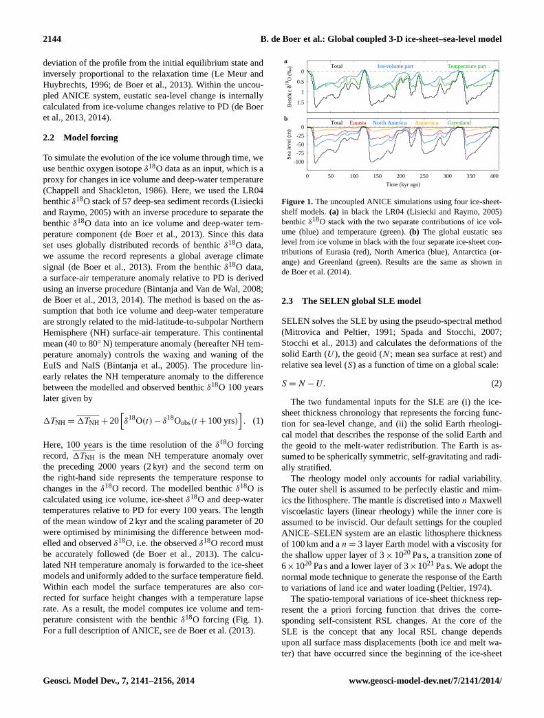
Here, 100 years is the time resolution of theδ18O forcingrecord,1TNH is the mean NH temperature anomaly overthe preceding 2000 years (2 kyr) and the second term onthe right-hand side represents the temperature response tochanges in theδ18O record. The modelled benthicδ18O iscalculated using ice volume, ice-sheetδ18O and deep-watertemperatures relative to PD for every 100 years. The lengthof the mean window of 2 kyr and the scaling parameter of 20were optimised by minimising the difference between mod-elled and observedδ18O, i.e. the observedδ18O record mustbe accurately followed (de Boer et al., 2013). The calcu-lated NH temperature anomaly is forwarded to the ice-sheetmodels and uniformly added to the surface temperature field.Within each model the surface temperatures are also cor-rected for surface height changes with a temperature lapserate. As a result, the model computes ice volume and tem-perature consistent with the benthicδ18O forcing (Fig.1).For a full description of ANICE, seede Boer et al.(2013).

0

0.5

1

1.5Ben

thic

δ18

O (

‰) Total Ice-volume part Temperature part

a

-100

-75

-50

-25

0

400350300250200150100500

Sea

leve

l (m

)

Time (kyr ago)

Total Eurasia North America Antarctica Greenlandb

Figure 1. The uncoupled ANICE simulations using four ice-sheet-shelf models.(a) in black the LR04 (Lisiecki and Raymo, 2005)benthicδ18O stack with the two separate contributions of ice vol-ume (blue) and temperature (green).(b) The global eustatic sealevel from ice volume in black with the four separate ice-sheet con-tributions of Eurasia (red), North America (blue), Antarctica (or-ange) and Greenland (green). Results are the same as shown inde Boer et al.(2014).

2.3 The SELEN global SLE model

SELEN solves the SLE by using the pseudo-spectral method(Mitrovica and Peltier, 1991; Spada and Stocchi, 2007;Stocchi et al., 2013) and calculates the deformations of thesolid Earth (U ), the geoid (N ; mean sea surface at rest) andrelative sea level (S) as a function of time on a global scale:

S = N − U. (2)

The two fundamental inputs for the SLE are (i) the ice-sheet thickness chronology that represents the forcing func-tion for sea-level change, and (ii) the solid Earth rheologi-cal model that describes the response of the solid Earth andthe geoid to the melt-water redistribution. The Earth is as-sumed to be spherically symmetric, self-gravitating and radi-ally stratified.

The rheology model only accounts for radial variability.The outer shell is assumed to be perfectly elastic and mim-ics the lithosphere. The mantle is discretised inton Maxwellviscoelastic layers (linear rheology) while the inner core isassumed to be inviscid. Our default settings for the coupledANICE–SELEN system are an elastic lithosphere thicknessof 100 km and an = 3 layer Earth model with a viscosity forthe shallow upper layer of 3× 1020 Pa s, a transition zone of6×1020 Pa s and a lower layer of 3×1021 Pa s. We adopt thenormal mode technique to generate the response of the Earthto variations of land ice and water loading (Peltier, 1974).

The spatio-temporal variations of ice-sheet thickness rep-resent the a priori forcing function that drives the corre-sponding self-consistent RSL changes. At the core of theSLE is the concept that any local RSL change dependsupon all surface mass displacements (both ice and melt wa-ter) that have occurred since the beginning of the ice-sheet



Figure 2. Scheme of the modelling framework. A coupling interval of 100 years is indicated by the black arrows, red arrows indicate acoupling every1tC = 1000 years. The model is forced with benthicδ18O data, from which a NH temperature anomaly1TNH is computedand forwarded to ANICE and the deep-water temperature module. ANICE computes the separate contributions of ice volume and deep-watertemperature to benthicδ18O, which are sent back to the inverse routine every 100 years (de Boer et al., 2013). Every 1000 years ANICEforwards grounded ice thickness, the Iceload given in the input array (IA), to SELEN, which computes the gravitationally self-consistent sealevel and bedrock topography adjustment that are coupled back to ANICE; in terms of the RSL,S is given in the output array (OA).

chronology anywhere on the Earth. Recent improvements ac-count for the dynamical feedback from the solid Earth rota-tion and the lateral migration of coastlines, also known as thetime-dependent ocean function (Milne and Mitrovica, 1996;Mitrovica and Milne, 2003; Kendall et al., 2005). We solvethe SLE with a pseudo-spectral numerical scheme (Spadaand Stocchi, 2007) that we truncate at a spherical harmonicdegree of order 128 to save computation time. Moreover, theSLE is solved by means of an iterative procedure where, atthe first iteration, the RSL changeS is assumed to be eu-static. After 3 iterations, the solution has converged andS isregionally varying (non-eustatic, non-globally uniform) ac-cording to GIA feedback (Farrell and Clark, 1976; Mitrovicaand Peltier, 1991; Spada and Stocchi, 2007),

3 The fully coupled system of ANICE–SELEN

In the following, we describe the dynamical interaction be-tween the four regional 3-D ice-sheet-shelf models, whichdefine the ANICE sub-system (see Sect.2.1), and the grav-itationally self-consistent SLE, which is solved by means ofSELEN (see Sect.2.3) as illustrated in Fig.2. In the cou-pled ANICE–SELEN system, the RSL change that is pro-vided to ANICE includes bedrock deformation and changesin the sea surface and thus replaces the regional ELRA modelthat is used for the stand-alone ANICE simulations. Accord-ing to the SLE, solid Earth and geoid deformation at eachpoint in space and time linearly depend on all the ice-sheetthickness variations and on the corresponding changes inthe ocean loading that have occurred until that time. Hav-ing ANICE–SELEN fully and dynamically coupled impliesthat information is exchanged between the two sub-systems

through time. ANICE provides SELEN with ice-sheet thick-ness variation in space and time, while SELEN returns thecorresponding RSL change (representing both variations inU and N , see Eq.2) to ANICE. The two means of com-munication between ANICE and SELEN are the input arrayIA(λ,θ), which carries information about ice-sheet thicknessvariation in space, and the output array OA(λ,θ), which re-trieves the RSL change at each element of the four ANICEsub-domains. Both are a function of latitude (λ) and longi-tude (θ). The output array, containing RSL change, is usedwithin ANICE to update the topography for the next timestep. This procedure is repeated with a coupling interval1tC= 1 kyr (Fig.2 and Table2). Before the coupling starts, AN-ICE is spun up for 1 glacial cycle in the uncoupled modewithout SELEN. In the uncoupled ANICE sub-system, eachregional ice-sheet model deforms its own regional topogra-phy independently from the other three ice sheets. Together,the four regional ice-sheet models contribute and respond tothe global eustatic sea-level change. The latter is internallycalculated from the changes in ice volume and is the onlymeans of connection among the four ice sheets. When thecoupling starts at 410 kyr ago, the ELRA model is switchedoff and all four regions use the spatially varying RSL as pro-vided by SELEN, which implicitly includes the deformationof the Earth.

3.1 Spatial discretisation

The execution of the algorithm starts with the discretisa-tion of the Earth surface into almost equal-area hexagonalelements. The number of hexagons, i.e. the spatial resolu-tion of the global mesh used within SELEN, depends on theparameter RES (Spada and Stocchi, 2007) (see AppendixA).



Table 2.Model parameters for time discretisation.

Parameter Description Value

1tC The coupling time interval 1 kyrNT Number of time steps of the moving time window 15L Total length of the moving time window 80 kyr1tS (NT) The time steps of the moving time window 10× 1, 2× 5, 3× 20 kyr

A RES value of 60 was adopted, which results in 141 612hexagonal elements, and each element approximately corre-sponds to a disc with a half amplitude ofα = 0.304 angulardegrees (see AppendixA). We employ the surface interpo-lation routine grdtrack from GMT (Wessel and Smith, 1991)to project ETOPO1 topography on the global mesh (Amanteand Eakins, 2009). For each element the grdtrack routine pro-vides a value for the bedrock topography as well as a valuefor the ice elevation that is non-zero wherever ice is cur-rently present. Wherever the bedrock height is negative andthe ice elevation is non-zero, we evaluate whether the ice isgrounded or floating. This is essential for defining the oceanfunction (OF), which describes if an element belongs to theocean (OF= 1) or to the land (OF= 0) (Milne et al., 2002).

Once the initial global topography file is generated, we up-date this field by projecting the four initial ANICE topogra-phies and ice-sheet thickness on the SELEN grid. However,the three Northern Hemisphere regional ice-sheets models(NaIS, EuIS and the GrIS) share overlapping regions. Wetherefore define a hierarchical procedure where the topogra-phy and ice-sheet thickness values to be interpolated on theelements of the global mesh are, firstly, those from the NaIS,secondly, the EuIS and, finally, the GrIS and AIS (see Sup-plement). The ANICE grid points and SELEN ice elementsare shown in Fig.3 and the specific number ofx andy gridpoints and SELEN elements of each ice-sheet model grid areprovided in Table1.

The geographical coordinates of the elements that areinitially updated with the four separate ANICE topogra-phies and ice-sheet thickness are stored in the input array.These are the elements that could potentially be affected byice-thickness variation through time, and consequently arerecognised by SELEN as ice-sheet elements (Fig.3b, d). Theice-sheet thickness is initially zero in ice free areas and non-zero wherever there is currently grounded ice, i.e. on Green-land and Antarctica. This initial array is the projection of to-pography and ice thickness of the four ANICE sub-domainson the global hexagonal mesh and represents an interglacialstage from which all of our simulations start. At each cou-pling time step1tC of the simulation, the array is updatedwith new ice-sheet thickness values according to ANICE,and the information is passed to SELEN for the computa-tion of the GIA-induced RSL changes. The latter are re-turned to ANICE by means of the output array that stores the

Figure 3. The four separate ANICE rectangular grid points for(a)the NH and(c) for Antarctica. The corresponding SELEN hexag-onal elements for(b) the NH and(d) Antarctica. The colours cor-respond to each ice sheet: blue – NaIS, red – EuIS, green – GrISand orange – AIS. The numbers of ANICE grid points and SELENelements are shown in Table1.

geographical coordinates of the centroids of the equal-areaelements of the four ice-sheet regions.

3.2 Temporal discretisation

In SELEN, the temporal discretisation is performed assum-ing that the variables vary stepwise in time (Spada and Stoc-chi, 2007). Usually, the late Pleistocene ice-sheet time histo-ries that are available from literature (e.g.Peltier, 2004) arediscretised into time steps of 500 or 1000 years. Providedthat the solid Earth behaves like a Maxwell viscoelastic body(see Sect.2.3), the RSL change induced by the ice thicknessvariation between two consecutive times accounts for (i) animmediate elastic part that occurs as soon as the second ice-sheet thickness is loaded and (ii) a viscous part that dependson the mantle viscosity profile and on the length of the timestep1tS, the time step at which the viscous response is dis-cretised.



When using SELEN for a prescribed a priori ice-sheetchronology, the spatio-temporal discretisation of ice-sheetthickness is assimilated at once (Spada and Stocchi, 2007).Consequently, given the time step1tS, the total number oftime steps and the load Love numbers (Peltier, 1974), theRSL change is computed by means of spatio-temporal convo-lutions over the surface of the Earth. Accordingly, the changein RSL at any location on the Earth and at any time sincethe beginning of the ice-sheet chronology is determined byall the ice and ocean load variations that have occurred untilthat time step (see Sect.2.3). This implies that, by assuminga predefined mantle viscosity profile, it is possible to com-pute RSL changes at any timet after the end of the ice-sheetchronology as a consequence of the mantle viscous relax-ation, which is an exponentially decaying function of time(Peltier, 1974).

When coupling ANICE–SELEN, a problem arises becausethe ice thickness variation through time is not known a priori.The ice-sheet thickness variation is only known until the timeSELEN is called by ANICE, which is done with an intervalof 1tC = 1 kyr. This implies that any time ANICE calls SE-LEN to compute the bedrock deformation and the sea-surfacevariation for a specific timet > −410 kyr (the first time thatANICE calls SELEN), all the deformations triggered by theprevious time steps are required. Hence, any timet SE-LEN is called, the SLE must be solved starting again fromt = −410 kyr (the first ice thickness change). As a conse-quence, the arrays carrying the SLE results grow throughoutthe simulations. This is not a big problem when simulatingshort ice-sheet fluctuations like the post LGM melting, butit is definitely a limitation when simulating multiple glacialcycles.

To avoid this problem, we take advantage of the linearityof both the SLE and of the rheological model. In particular,we use the fact that the viscous response of the bedrock de-formation exponentially decays with time and ceases onceisostatic equilibrium has been reached. At any timet whenANICE calls SELEN, the bedrock deformationU(t) and thegeoid changeN(t), due to the ice-thickness changeI (t) =

H(t) − H(t − 1tS), are computed betweent = t + 1tS anda predefinedt = L, whereL is the total length (in kyr) ofa moving time window (see Table2). Here,H(t) is the icethickness at timet , andI (t) is the change in ice thicknessrelative to the previous time step.

We call this temporal discretisation scheme the “movingtime window”. The length of the moving time windowL, i.e.how far into the future SELEN solves for the RSL change,is a free parameter. The longer the moving time window, themore accurate the results will be, because more informationfrom the past is taken into account. In order to maintain along enough moving time window and to save CPU time, itis important to consider how many time steps NT (Number oftime steps of the moving time window) of1tS are used to de-fine the moving window. If the length of the moving window

Figure 4. Bedrock deformation according to a sequential increaseof ice thickness on the south pole (Fig.5) at a colatitude of 18◦. Ev-ery 1 kyr the ice thickness is increased with 20 m, any 20 m increaseof ice thickness contributes to 80 kyr of viscoelastic crustal defor-mation.(a) At t = 1 kyr the predicted bedrock deformation at the15 time steps of the moving time window.(b) Light grey markersindicate the fully discretised solution that is stored at1tC =1 kyrresolution.(c) The predicted deformation for five consecutive timesteps. The total solution, including past deformations and the elasticresponse is shown in red. Insets for panels(a)–(c) show the impliedice thickness variations, steps of 20 m per 1 kyr.

allows for a longer memory, the number of time steps allowfor an accurate discretisation of the RSL change.

Figure4 illustrates this process for a 20 m thick ice sheetthat is added at timet = 0 (inset of Fig.4a; using a schematicset-up as shown in Fig.5). SELEN computes the bedrockdeformation fromt = 0 to t = L, the length of the movingtime window that is set toL = 80 kyr. The bedrock deforma-tion is computed at NT= 15 time points in the future, withNT the number of time steps1tS of the moving time win-dow (see Table2). The time steps are heterogeneous, i.e. 10steps of 1 kyr, 2 steps of 5 kyr and 3 steps of 20 kyr. The dis-cretisation time step1tS is thus an array of length NT= 15.The black squares show the predicted bedrock deformationat each time step. Then, the bedrock deformation is interpo-lated within the total window of 80 kyr to have a discretisedsolution at the resolution of the coupling interval1tC = 1 kyr(Fig. 4b). At the following timet = t +1tC, another 20 m ofice is added above the initial ice layer, and the bedrock defor-mation due to this extra mass is computed again in the sameway. The new array is summed to the previous one to incor-porate the viscous deformations of the initial ice-thicknessvariation (Fig.4c). This process is carried on throughout the



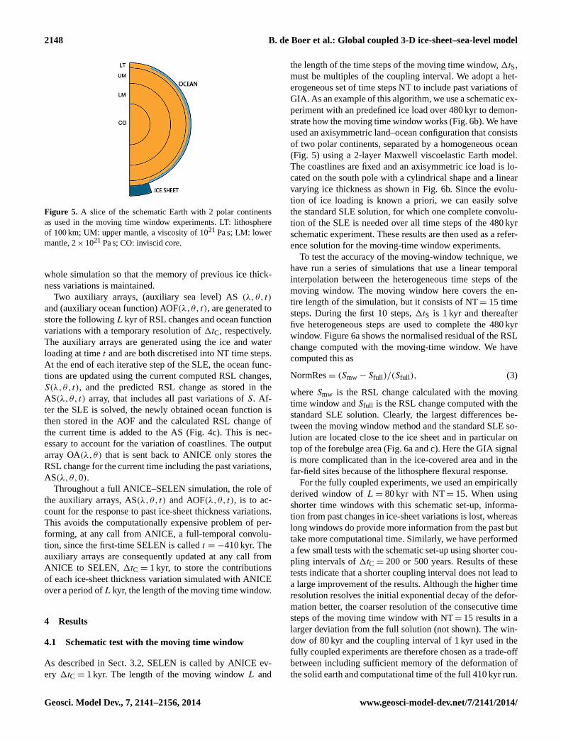
Figure 5. A slice of the schematic Earth with 2 polar continentsas used in the moving time window experiments. LT: lithosphereof 100 km; UM: upper mantle, a viscosity of 1021Pa s; LM: lowermantle, 2× 1021Pa s; CO: inviscid core.

whole simulation so that the memory of previous ice thick-ness variations is maintained.

Two auxiliary arrays, (auxiliary sea level) AS(λ,θ, t)

and (auxiliary ocean function) AOF(λ,θ, t), are generated tostore the followingL kyr of RSL changes and ocean functionvariations with a temporary resolution of1tC, respectively.The auxiliary arrays are generated using the ice and waterloading at timet and are both discretised into NT time steps.At the end of each iterative step of the SLE, the ocean func-tions are updated using the current computed RSL changes,S(λ,θ, t), and the predicted RSL change as stored in theAS(λ,θ, t) array, that includes all past variations ofS. Af-ter the SLE is solved, the newly obtained ocean function isthen stored in the AOF and the calculated RSL change ofthe current time is added to the AS (Fig.4c). This is nec-essary to account for the variation of coastlines. The outputarray OA(λ,θ) that is sent back to ANICE only stores theRSL change for the current time including the past variations,AS(λ,θ,0).

Throughout a full ANICE–SELEN simulation, the role ofthe auxiliary arrays, AS(λ,θ, t) and AOF(λ,θ, t), is to ac-count for the response to past ice-sheet thickness variations.This avoids the computationally expensive problem of per-forming, at any call from ANICE, a full-temporal convolu-tion, since the first-time SELEN is calledt = −410 kyr. Theauxiliary arrays are consequently updated at any call fromANICE to SELEN,1tC = 1 kyr, to store the contributionsof each ice-sheet thickness variation simulated with ANICEover a period ofL kyr, the length of the moving time window.

4 Results

4.1 Schematic test with the moving time window

As described in Sect.3.2, SELEN is called by ANICE ev-ery 1tC = 1 kyr. The length of the moving windowL and

the length of the time steps of the moving time window,1tS,must be multiples of the coupling interval. We adopt a het-erogeneous set of time steps NT to include past variations ofGIA. As an example of this algorithm, we use a schematic ex-periment with an predefined ice load over 480 kyr to demon-strate how the moving time window works (Fig.6b). We haveused an axisymmetric land–ocean configuration that consistsof two polar continents, separated by a homogeneous ocean(Fig. 5) using a 2-layer Maxwell viscoelastic Earth model.The coastlines are fixed and an axisymmetric ice load is lo-cated on the south pole with a cylindrical shape and a linearvarying ice thickness as shown in Fig.6b. Since the evolu-tion of ice loading is known a priori, we can easily solvethe standard SLE solution, for which one complete convolu-tion of the SLE is needed over all time steps of the 480 kyrschematic experiment. These results are then used as a refer-ence solution for the moving-time window experiments.

To test the accuracy of the moving-window technique, wehave run a series of simulations that use a linear temporalinterpolation between the heterogeneous time steps of themoving window. The moving window here covers the en-tire length of the simulation, but it consists of NT= 15 timesteps. During the first 10 steps,1tS is 1 kyr and thereafterfive heterogeneous steps are used to complete the 480 kyrwindow. Figure6a shows the normalised residual of the RSLchange computed with the moving-time window. We havecomputed this as

NormRes= (Smw − Sfull )/(Sfull ), (3)

whereSmw is the RSL change calculated with the movingtime window andSfull is the RSL change computed with thestandard SLE solution. Clearly, the largest differences be-tween the moving window method and the standard SLE so-lution are located close to the ice sheet and in particular ontop of the forebulge area (Fig.6a and c). Here the GIA signalis more complicated than in the ice-covered area and in thefar-field sites because of the lithosphere flexural response.

For the fully coupled experiments, we used an empiricallyderived window ofL = 80 kyr with NT= 15. When usingshorter time windows with this schematic set-up, informa-tion from past changes in ice-sheet variations is lost, whereaslong windows do provide more information from the past buttake more computational time. Similarly, we have performeda few small tests with the schematic set-up using shorter cou-pling intervals of1tC = 200 or 500 years. Results of thesetests indicate that a shorter coupling interval does not lead toa large improvement of the results. Although the higher timeresolution resolves the initial exponential decay of the defor-mation better, the coarser resolution of the consecutive timesteps of the moving time window with NT= 15 results in alarger deviation from the full solution (not shown). The win-dow of 80 kyr and the coupling interval of 1 kyr used in thefully coupled experiments are therefore chosen as a trade-offbetween including sufficient memory of the deformation ofthe solid earth and computational time of the full 410 kyr run.



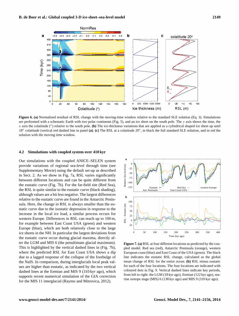
Figure 6. (a) Normalised residual of RSL change with the moving-time window relative to the standard SLE solution (Eq.3). Simulationsare performed with a schematic Earth with two polar continents (Fig.5), and an ice sheet on the south pole. They axis shows the time, thex axis the colatitude (◦) relative to the south pole.(b) The ice-thickness variations that are applied as a cylindrical shaped ice sheet up until18◦ colatitude (vertical red dashed line in panel(a). (c) The RSL at a colatitude 20◦, in black the full standard SLE solution, and in red thesolution with the moving time window.

4.2 Simulations with coupled system over 410 kyr

Our simulations with the coupled ANICE–SELEN systemprovide variations of regional sea-level through time (seeSupplementary Movie) using the default set-up as describedin Sect.2. As we show in Fig.7a, RSL varies significantlybetween different locations and can be quite different fromthe eustatic curve (Fig.7b). For the far-field site (Red Sea),the RSL is quite similar to the eustatic curve (black shading),although values are a bit less negative. The largest differencesrelative to the eustatic curve are found in the Antarctic Penin-sula. Here, the change in RSL is always smaller than the eu-static curve due to the isostatic depression in response to theincrease in the local ice load, a similar process occurs forwestern Europe. Differences in RSL can reach up to 100 m,for example between East Coast USA (green) and westernEurope (blue), which are both relatively close to the largeice sheets in the NH. In particular the largest deviations fromthe eustatic curve occur during glacial maxima, directly af-ter the LGM and MIS 6 (the penultimate glacial maximum).This is highlighted by the vertical dashed lines in (Fig.7b),where the predicted RSL for East Coast USA shows a dipdue to a lagged response of the collapse of the forebulge ofthe NaIS. In comparison, during interglacials local peak val-ues are higher than eustatic, as indicated by the two verticaldashed lines at the Eemian and MIS 9 (310 kyr ago), whichsupports recent numerical simulation of the GIA correctionfor the MIS 11 interglacial (Raymo and Mitrovica, 2012).

-125

-100

-75

-50

-25

0

Rel

ativ

e Se

a le

vel (

m)

a

EustaticAnt. Peninsula

Red SeaEast Coast USA

western Europe

-25

0

25

50

75

100

400350300250200150100500

RSL

- E

usta

tic (

m)

Time (kyr ago)

b

Figure 7. (a)RSL at four different locations as predicted by the cou-pled model. Red sea (red), Antarctic Peninsula (orange), westernEuropean coast (blue) and East Coast of the USA (green). The blackline indicates the eustatic RSL change, calculated as the globalmean change of RSL for the entire ocean.(b) RSL minus eustaticfor each of the four locations. The four locations are indicated withcoloured dots in Fig.9. Vertical dashed lines indicate key periods,from left to right: the LGM (18 kyr ago), Eemian (122 kyr ago), ma-rine isotope stage (MIS) 6 (138 kyr ago) and MIS 9 (310 kyr ago).



4.3 Comparison with the eustatic solution

The initial set-up of the ANICE model as described inde Boer et al.(2013) calculates the change in sea level fromthe eustatic contributions of the four ice sheets relative toPD. In Fig.1b, the four contributions of the ice sheets areshown over the 410 kyr time period. Clearly, the largest con-tributions arise from the NH ice sheets on Eurasia and NorthAmerica. When we include the regional sea-level variations,the local evolution of ice thickness will obviously change dueto the self-gravitation effect, especially for the marine partsof the ice sheets.

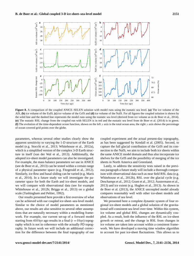
In Fig. 8a–d, we compare the modelled ice volume of thecoupled ANICE–SELEN simulation with a simulation thatis not coupled to SELEN (ice volume fromde Boer et al.,2014). The largest differences occur during the glacial peri-ods, especially for the AIS (Fig.8a). For Antarctica, thesedifferences are mainly observed in the marine sectors of theice sheet, i.e. West Antarctica. Here, including the gravita-tionally self-consistent sea-level change reduces the growthof the ice sheet relative to the non-coupled run. As a result,with only eustatic variations (dashed line in Fig.8a), the icesheet grows significantly larger during a glacial period. Thusby including the self-gravitation effects and RSL changes,the growth of the West Antarctic ice sheet results in a localincrease of sea level rather than a eustatic fall, which inducesa slower advance of the ice sheet and thus a smaller ice vol-ume. This self-stabilisation mechanism has been identifiedpreviously in coupled model simulations for Antarctica byGomez et al.(2013).

The gravitationally self-consistent solution of the SLEprovides a much more realistic behaviour of the response ofthe solid Earth to changes in ice and water loading. The vis-coelastic Earth model accounts for the response on multipletimescales and provides a global solution, whereas a singleresponse timescale of 3 kyr is used in the uncoupled solutionof ANICE. For all four ice sheets (Fig.8a–d), our currentset-up of SELEN provides a lower response of the bedrockrelative to the flexural Earth model used in the uncoupledANICE simulation (dashed lines). This results in a lower to-tal ice volume for the coupled solution, especially for theNaIS (Fig.8d). Because the coupled simulation takes intoaccount the change of the coastline over the globe (i.e. thetime-dependent ocean function), the area of the total oceanis reduced by about 5 % of the global surface area duringglacial maxima (Fig.8f). Consequently, the total eustatic sea-level change of the two simulations (Fig.8e) is coincidentallyquite similar over the whole 410 kyr period.

4.4 Rotational feedback

An important aspect of the gravitationally self-consistent so-lution of the SLE is the rotational feedback, which is a newfeature in SELEN. The changes in the mass distribution of iceand water induce a shift in the position of the rotational axis

(polar wander) that has an ellipsoidal form (e.g.Gomez et al.,2010b). The difference as shown in Fig.9b is described bythe spherical harmonics of degree 2 (e.g.Mound and Mitro-vica, 1998) (see also the Supplement Movie). As is shownin Fig. 9b, the positive contribution of the degree 2 signalis centred in the North Atlantic ocean and is related to thelarge increase in ice volume in the NH, which thus adds sev-eral metres to the fall in sea level during the LGM. These re-gional differences result in differences in the local ice thick-ness (Fig.9d), but a minimal change in total ice volume. Theaddition of the rotation feedback, which is a significant con-tribution to the RSL change reaching up to 5 m or higher(Fig. 9b), is required for the correct interpretation of RSLdata. In addition, there is a clear dynamical response of theice sheets (Fig.9d) to the differences in RSL, which resultsin large and significant changes in local RSL values close tothe ice sheets.

5 Discussion and conclusions

In this paper we have presented a fully and dynamicallycoupled system of four 3-D ice-sheet-shelf models (de Boeret al., 2013, 2014) and a glacial isostatic adjustment modelbased on the SLE (Spada and Stocchi, 2007). The two key as-pects of the coupling algorithm are the spatial discretisationand related interpolation of the ice volume from the four dif-ferent regional ice-sheet-shelf models, and the temporal dis-cretisation scheme with the related time interpolation. Thissystem is the first fully coupled global ice-sheet–sea-levelmodel available. Here, we have provided a simulation of theglobal solution of ice volume and relative sea-level variationsover the past four glacial cycles.

The key aspect of our results is the dynamical responseof the ice sheets to changes in RSL, which includes boththe deformation of the bedrock in response to ice and wa-ter loading and the geoidal deformations. When an ice sheetgrows, due to the self-gravitational pull of the ice sheet theRSL close to the ice sheets actually rises, whereas the globalmean sea level falls. The self-gravitational pull thus acts tostabilise the ice sheets, as has also been shown byGomezet al. (2013) with a coupled ice-sheet–sea-level model forAntarctica. Henceforth, ice volume is lower during glacialperiods. Overall the coupled model results in lower ice vol-ume relative to an uncoupled simulation that uses eustaticsea level derived from ice-volume changes only. We alsoinclude a time-dependent ocean function that accounts forthe changes in the coastlines over the globe. This leads toa significant reduction in the ocean area during the glacialmaxima and hence results in a nearly equal eustatic sea-levelchange compared to the uncoupled simulations.

The use of the 3-layer Maxwell viscoelastic Earth modelgives a lower response in bedrock deformation due to the iceloading relative to the simplified model used in earlier stud-ies (de Boer et al., 2013). We use one set of Earth model



24

26

28

30

AIS

ice

volu

me

(106 k

m3 ) a

2.3

2.6

2.9

3.2

GrI

S ic

e vo

lum

e (1

06 km

3 ) c

-100

-75

-50

-25

0

400350300250200150100500

Eus

tatic

RSL

cha

nge

(m)

Time (kyr ago)

e

4

8

12

16

EuI

S ic

e vo

lum

e (1

06 km

3 ) b

6

12

18

24

NaI

S ic

e vo

lum

e (1

06 km

3 ) d

340

345

350

355

360

400350300250200150100500

66

67.5

69

70.5

72

Oce

an a

rea

(106 k

m2 )

Oce

an a

rea

(%)

Time (kyr ago)

f

Figure 8. A comparison of the coupled ANICE–SELEN solution with model runs using the eustatic sea level.(a) The ice volume of theAIS, (b) ice volume of the EuIS,(c) ice volume of the GrIS and(d) ice volume of the NaIS. For all figures the coupled solution is shown bythe solid line and the dashed line represents the model runs using the eustatic sea level (derived from ice volume as inde Boer et al., 2014).(e) The eustatic RSL change from the coupled run with SELEN is in red and the eustatic sea level fromde Boer et al.(2014) is in green.(f) The evolution of the time-dependent ocean function, shown on the lefty axis is the total ocean area, the righty axis shows the percentageof ocean covered grid points over the globe.

parameters, whereas several other studies clearly show theapparent sensitivity to varying the 1-D structure of the Earthmodel (e.g.Stocchi et al., 2013; Whitehouse et al., 2012a),which is a simplified version of the complex 3-D Earth struc-ture in itself (van der Wal et al., 2013). Additionally, theadopted ice-sheet model parameters can also be investigated.For example, the mass balance parameters we use in ANICE(seede Boer et al., 2013) can be tested within a certain rangeof a physical parameter space (e.g.Fitzgerald et al., 2012).Similarly, ice flow and basal sliding can be varied (e.g.Mariset al., 2014). In a future study we will investigate the pa-rameter space for both the Earth and ice-sheet models, andwe will compare with observational data (see for exampleWhitehouse et al., 2012b; Briggs et al., 2013) on a globalscale (Tushingham and Peltier, 1992).

Our results presented here provide a first overview of whatcan be achieved with our coupled ice-sheet–sea-level model.Similar to the choice of model parameters as mentionedabove, our results are also sensitive to several other assump-tions that are naturally necessary within a modelling frame-work. For example, our current set-up of a forward modelstarting from 410 kyr ago results in a final (t = 0 kyr) topog-raphy which is not in coherence with the actually PD topog-raphy. In future work we will include an additional correc-tion for the difference between the final topography of our

coupled experiment and the actual present-day topography,as has been suggested byKendall et al.(2005). Second, tocapture the full glacial contribution of the GrIS and its con-nection to the NaIS, we aim to include both ice sheets withinthe same ANICE model domain and thus also incorporate iceshelves for the GrIS and the possibility of merging of the icesheets in North America and Greenland.

Lastly, to address the sensitivity tests raised in the previ-ous paragraph a future study will include a thorough compar-ison with observational data such as near field RSL data (e.g.Whitehouse et al., 2012b), RSL over the glacial cycle (e.g.Deschamps et al., 2012; Grant et al., 2012; Austermann et al.,2013) and ice extent (e.g.Hughes et al., 2013). As shown inde Boer et al.(2013), the ANICE uncoupled model alreadycompares reasonably well with other ice-sheet models andobservations of sea level.

We presented here a complete dynamic system of four re-gional ice-sheet models and a global solution of the gravita-tional self-consistent sea level over time. Within this system,ice volume and global RSL changes are dynamically cou-pled. As a result, both the influence of the RSL on ice-sheetgrowth or retreat, and the change in RSL from changes inice volume are taken into account within a consistent frame-work. We have developed a moving time window algorithmto account for past ice-sheet fluctuations. This allows us to



Figure 9.Results of a coupled ANICE–SELEN run at the last glacial maximum (here 18 kyr ago).(a) RSL change with respect to the eustatic(= 111.3 m below PD) including rotational feedback.(b) The difference in RSL of a run using rotational feedback (as ina) with a run withoutrotational feedback.(c) The total ice loading from ANICE (= 112.8 m s.e.) including rotational feedback.(d) The difference in ice loading ofa run using rotational feedback (as inc) with a run without rotational feedback. In panela the coloured dots indicate the locations illustratedin Fig. 7. A full time evolution of the 410 kyr long simulation of these maps is shown in the Supplement Movie.

calculate RSL and ice volume over the globe over four glacialcycles, starting 410 kyr ago. Our simulations show that espe-cially during periods of rapid changes of sea level relativeto PD, differences between regions can be very large; thus,showing the importance of this coupled system for model–data comparison on a regional scale.



Appendix A: Spatial discretisation of SELEN

The SLE requires a global discretisation of both the surfaceice loads (and consequently of the oceanic counterpart, i.e.melt water loading), topography and bathymetry. Therefore,it is necessary to merge the four sub-domains of ANICE intoa global field. FollowingSpada and Stocchi(2007), we firstgenerate an initial global mask discretised into equal-areahexagonal elements (i.e. pixels). The number of pixels (NP),which defines the resolution of the mask, depends on the pa-rameter RES (Spada and Stocchi, 2007):

NP= 2× RES× (RES− 1) × 20+ 12. (A1)

In this paper we set RES= 60, which results in141 612 pixels. We plot on this mask the values of topog-raphy (both for bedrock and ice elevation) from the high-resolution ETOPO1 model (Amante and Eakins, 2009). Forthis purpose the ETOPO1 topographic values are first inter-polated on a global 0.1◦

× 0.1◦ rectangular grid. Each ele-ment is then transformed to an equivalent-area spherical capof radiusα:

α(λ,θ) = arccos

[1− sin(90− λ) × sin

β

2×

β

180

], (A2)

whereβ = 0.1◦. Similarly, the NP pixels of the global meshare converted into equal-area spherical caps of radius:

αsle = (180/π) ×√

4/NP. (A3)

With RES= 60, the radius for the global mesh isαsle =

0.3. To assign at each pixel a value that corresponds to theETOPO1 topography, we evaluate the intersections betweenthe pixels and the disk elements from the ETOPO1 conver-sion. For this purpose we employ the method described byTovchigrechko and Vakser(2001). For each pixel, we sumpositive (above mean sea level, i.e. land) and negative (belowmean sea level, i.e. sea bottom) volumes, using a weightedaverage. The same is done for the grounded ice. To check ifthe ice point is still grounded, we evaluate whether the topog-raphy is positive or negative. At first, despite the thickness ofthe ice, the pixel is considered land, and a value of 0 is as-signed to the OF. If the topography is negative, we compare

Table A1. Example of pixels of the global mesh with the assigned values of the functions. OF: ocean function, FGI: floating or grounded ice,AOF: auxiliary ocean function (i.e. the time-dependent ocean function), m.s.l.: mean sea level.

Long Lat Topo OF Ice FGI AOF(◦ E) (◦ N) (m) (m) OF× FGI

(1) above m.s.l., ice free 50.0 40.0 +250.0 0 0.0 1 0(2) above m.s.l., ice covered 320.0 70.0 +500.0 0 750.0 0 0(3) below m.s.l., ice free 50.0 40.0 −850.0 1 0.0 1 1(4) below m.s.l., grounded ice 50.0 40.0 −100.0 1 550.0 0 0(5) below m.s.l., floating ice 50.0 40.0 −350.0 1 50.0 1 1

the thickness of the ice with the absolute value of bathymetry,considering the density ratio between ice and water, we eval-uate if the ice is grounded or floating. As a result, we gen-erate a global topography/bathymetry file based on the origi-nal ETOPO1 (Amante and Eakins, 2009). For each pixel thefollowing values are assigned: longitude, latitude, longitudeanchor, latitude anchor, OF label, topography, ice thicknesslabel and ice thickness (see TableA1). Furthermore, it is im-portant to keep in mind that according to our discretisation,lakes, ponds and enclosed basins are considered as part of the(global) ocean function.

The global topography must now be updated for the fourregions considered by ANICE (North America, Eurasia,Greenland and Antarctica). Of course there are overlappingregions. This is done in a sequential order, starting fromNorth America, then Eurasia, then Greenland and finallyAntarctica (see Supplement). For converting the ice thicknesson the rectangular grid points of ANICE on to the SELENpixels, we account for conservation of ice volume for eachgrid point. Similar to the initial topography from ETOPO1,the rectangular grid points are first converted into discs withradius:

αice =1x

RE√

π, (A4)

with the radius of the EarthRE = 6371.221 km. First, the to-tal overlapping area of each ANICE grid point is calculatedfor all SELEN elements. Second, the total volume for eachice covered SELEN element is corrected for the correspond-ing volume on the (original) ANICE rectangular grid point.Lastly, the interpolated ice thickness is calculated from thevolume divided by the area of the SELEN element. This rou-tine is included as Supplement.



Author contributions.The model code was developed by B. deBoer and P. Stocchi, coupled simulations were performed by B.de Boer. P. Stocchi performed the time window tests. R. S. W. vande Wal initiated the project, B. de Boer and P. Stocchi contributedequally to the writing of this manuscript. All authors contributed tothe discussion of the results and implications and commented on themanuscript at all stages.

The Supplement related to this article is available online atdoi:10.5194/gmd-7-2141-2014-supplement.

Acknowledgements.Part of this work was supported by COST Ac-tion ES0701 “Improved constraints on models of Glacial IsostaticAdjustment”. DynaQlim. NWO. Financial support for B. de Boerwas provided through the Royal Netherlands Academy of Artsand Sciences (KNAW) professorship of J. Oerlemans and NWOVICI grant of L. J. Lourens. Model runs were performed on theLISA Computer Cluster, we would like to acknowledge SurfSARAComputing and Networking Services for their support. The authorswould like to thank Pippa Whitehouse and an anonymous reviewerfor two very constructive reviews that significantly improved themanuscript. Sarah Bradley is thanked for her helpful comments.

Edited by: A. Le Brocq

References

Amante, C. and Eakins, B. W.: ETOPO1 1 Arc-Minute GlobalRelief Model: Procedures, Data Sources and Analysis, NOAATechnical Memorandum NESDIS NGDC-24, p. 19, 2009.

Austermann, J., Mitrovica, J. X., Latychev, K., and Milne, G. A.:Barbados-based estimate of ice volume at Last Glacial Maximumaffected by subducted plate, Mat. Geosci., 7, 553–557, 2013.

Bamber, J. L., Layberry, R. L. and Gogineni, S. P.: A new ice thick-ness and bed data set for the Greenland ice sheet 1. Measure-ments, data reduction, and errors, J. Geophys. Res., 106, 33733–33780, 2001.

Bard, E., Hamelin, B., and Fairbanks, R.: Deglacial sea-level recordfrom Tahiti corals and the timing of global meltwater discharge,Nature, 382, 241–244, 1996.

Bard, E., Hamelin, B., and Delanghe-Sabatier, D.: Meltwater pulse1B and Younger Dryas sea levels revisited with boreholes atTahiti, Deglacial, 327, 1235–1237, 2010.

Bassett, S. E., Milne, G. A., and Mitrovica, J. X., and Clark, P. U.:Ice Sheet and Solid Earth Influences on Far-Field Sea-Level His-tories, Science, 309, 925–928, 2005.

Becker, J. J., Sandwell, D. T., Smith, W. H. F., Braud, J., Binder, B.,Depner, J., Fabre, D., Factor, J., Ingalls, S., Kim, S.-H., Ladner,R., Marks, K., Nelson, S., Pharaoh, A., Trimmer, R., Von Rosen-berg, J., Wallace, G., and Weatherall, P.: Global Bathymetry andElevation Data at 30 Arc Seconds Resolution: SRTM30_PLUS,Marine Geodesy, 32, 355–371, 2009.

Bintanja, R. and Van de Wal, R. S. W.: North American ice-sheetdynamics and the onset of 100,000-year glacial cycles, Nature,454, 869–872, 2008.

Bintanja, R., Van de Wal, R. S. W., and Oerlemans, J.: Modelled at-mospheric temperatures and global sea level over the past millionyears, Nature, 437, 125–128, 2005.

Briggs, R., Pollard, D., and Tarasov, L.: A glacial systems modelconfigured for large ensemble analysis of Antarctic deglacia-tion, The Cryosphere, 7, 1949–1970, doi:10.5194/tc-7-1949-2013, 2013.

Chappell, J. and Shackleton, N. J.: Oxygen isotopes and sea level,Nature, 324, 137–140, 1986.

Clark, P. U., Mitrovica, J. X., Milne, G. A., and Tamisiea, M. E.:Sea-Level Fingerprinting as a Direct Test for the Source ofGlobal Meltwater Pulse IA, Science, 295, 2438–2441, 2002.

de Boer, B., van de Wal, R. S. W., Lourens, L. J., and Bintanja,R.: A continuous simulation of global ice volume over the past1 million years with 3-D ice-sheet models, Clim. Dynam., 41,1365–1384, 2013.

de Boer, B., Lourens, L. J., and van de Wal, R. S. W.: Persistent400,000-year variability of Antarctic ice volume and the carbon-cycle is revealed throughout the Plio-Pleistocene, Nat. Commun.,5, 2999, doi:10.1038/ncomms3999, 2014.

Denton, G. H., Anderson, R. F., Toggweiler, J. R., Edwards, R. L.,Schaefer, J. M., and Putnam, A. E.: The Last Glacial Termina-tion, Science, 328, 1652–1656, 2010.

Deschamps, P., Durand, N., Bard, E., Hamelin, B., Camoin, G.,Thomas, A. L., Henderson, G. M., Okuno, J., and Yokoyama,Y.: Ice-sheet collapse and sea-level rise at the Bolling warming14,600 years ago, Nature, 483, 559–564, 2012.

Ehlers, J. and Gibbard, P. L.: The extent and chronology of Ceno-zoic global glaciation, Quaternary International, 164–165, 6–20,2007.

Engelhart, S., Peltier, W., and Horton, B.: Holocene relative sea–level changes and glacial isostatic adjustment of the US Atlanticcoast, Geology, 39, 751–754, 2011.

Fairbanks, R. G.: A 17,000 year glacio–eustatic sea–level record:Influence of glacial melting rates on the Younger Dryas eventand deep ocean circulation, Nature, 342, 637–642, 1989.

Fairbridge, R. W.: Eustatic changes in sea level, Phys. Chem. Earth,5, 99–185, 1961.

Farrell, W. E. and Clark, J. A.: On postglacial sea level, Geophys. J.Roy. Astronom. Soc., 46, 647–667, 1976.

Fitzgerald, P. W., Bamber, J. L., Ridley, J. K., and Rougier, J. C.:Exploration of parametric uncertainty in a surface mass balancemodel applied to the Greenland ice sheet, J. Geophys. Res., 117,F01021, doi:10.1029/2011JF002067, 2012.

Gomez, N., Mitrovica, J. X., Huybers, P., and Clark, P. U.: Sea levelas a stabilizing factor for marine-ice-sheet grounding lines, Nat.Geosci., 3, 850–853, 2010a.

Gomez, N., Mitrovica, J. X., Tamisiea, M. E., and Clark, P. U.: Anew projection of sea level change in response to collapse of ma-rine sectors of the Antarctic Ice Sheet, Geophys. J. Int., 180, 623–634, 2010b.

Gomez, N., Pollard, D., and Mitrovica, J. X.: A 3-D coupled icesheet –sea level model applied to Antarctica through the last 40ky, Earth Planet. Sci. Lett., 384, 88–99, 2013.

Grant, K. M., Rohling, E. J., Bar-Matthews, M., Ayalon, A.,Medina-Elizalde, M., Bronk Ramsey, C., Satow, C., and Roberts,A. P.: Rapid coupling between ice volume and polar temperatureover the past 150,000 years, Nature, 491, 744–747, 2012.


http://dx.doi.org/10.5194/gmd-7-2141-2014-supplement

http://dx.doi.org/10.5194/tc-7-1949-2013

http://dx.doi.org/10.5194/tc-7-1949-2013

http://dx.doi.org/10.1038/ncomms3999

http://dx.doi.org/10.1029/2011JF002067


Hughes, P. D., Gibbard, P. L., and Ehlers, J.: Timing of glaciationduring the last glacial cycle: evaluating the concept of global“Last Glacial Maximum” (LGM), Earth-Sci. Rev., 125, 171–198,2013.

Hutter, L.: Theoretical Glaciology, D. Reidel, Dordrecht, 1983.Huybrechts, P.: Sea-level changes at the LGM from ice-dynamic

reconstructions of the Greenland and Antarctic ice sheets duringthe glacial cycles, Quaternary Sci. Rev., 21, 203–231, 2002.

Kendall, R. A., Mitrovica, J. X., and Milne, G. A.: On post-glacialsea level – II. Numerical formulation and comparative results onspherically symmetric models, Geophys. J. Int., 161, 679–706,2005.

Lambeck, K., Johnston, P., and Nakada, M.: Holocene glacial re-bound and sea-level change in NW Europe, Geophys. J. Int., 103,451–468, 1990.

Le Brocq, A. M., Payne, A. J., and Vieli, A.: An improvedAntarctic dataset for high resolution numerical ice sheet mod-els (ALBMAP v1), Earth Syst. Sci. Data, 2, 247–260, 2010,http://www.earth-syst-sci-data.net/2/247/2010/.

Le Meur, E. and Huybrechts, P.: A comparision of different waysof dealing with isostacy: examples from modelling the Antarcticice sheet during the last glacial cycle, Ann. Glaciol., 23, 309–317, 1996.

Lisiecki, L. and Raymo, M.: A Pliocene-Pleistocene stack of 57globally distributed benthicδ18O records, Paleoceanography, 20,PA1003, doi:10.1029/2004PA001071, 2005.

Maris, M. N. A., de Boer, B., Ligtenberg, S. R. M., Crucifix, M., vande Berg, W. J., and Oerlemans, J.: Modelling the evolution of theAntarctic ice sheet since the last interglacial, The Cryosphere, 8,1347–1360, doi:10.5194/tc-8-1347-2014, 2014.

Milne, G. and Mitrovica, J.: Postglacial sea-level change ona rotating Earth: first results from a gravitationally self-consistent sea-level equation, Geophys. J. Int., 126, F13–F20,doi:10.1111/j.1365-246X.1996.tb04691.x, 1996.

Milne, G. and Mitrovica, J.: Searching for eustasy in deglacial sea-level histories, Quaternary Sci. Rev., 25–26, 2292–2302, 2008.

Milne, G., Davis, J., Mitrovica, J., Scherneck, H., Johansson, J.,Vermeer, M., and Koivula, H.: Space-Geodetic Constraints onGlacial Isostatic Adjustment in Fennoscandia, Science, 291,2381–2385, 2001.

Milne, G. A., Mitrovica, J. X., and Schrag, D. P.: Estimating pastcontinental ice volume from sea-level data, Quaternary Sci. Rev.,21, 361–376, 2002.

Mitrovica, J. and Milne, G.: On post-glacial sea level: I. Generaltheory, Geophys. J. Int., 154, 253–267, 2003.

Mitrovica, J. X. and Peltier, W. R.: On post–glacial geoid subsi-dence over the equatorial ocean, J. Geophys. Res., 96, 20053–20071, 1991.

Morland, L. W.: Unconfined ice-shelf flow, in: Dynamics of theWest Antarctic Ice Sheet, edited by: de Veen, C. J. V. and Oerle-mans, J., 99–116, D. Reidel, 1987.

Mound, J. E. and Mitrovica, J. X.: True Polar Wander as a Mecha-nism for Second-Order Sea-Level Variations, Science, 279, 534–537, 1998.

Peltier, W. R.: The impulse response of a Maxwell Earth, Rev. Geo-phys. Space Phys., 12, 649–669, 1974.

Peltier, W. R.: Global Glacial Isostasy and the Surface of the Ice-Age Earth: The ICE-5G (VM2) model and GRACE, Annu. Rev.Earth Planet Sci., 32, 111–149, 2004.

Peltier, W. R. and Fairbanks, R. G.: Global glacial ice volume andLast Glacial Maximum duration from an extended Barbados sealevel record, Quaternary Sci. Rev., 25, 3322–3337, 2006.

Pirazzoli, P. A.: World atlas of Holocene sea level changes, Elsevier,Amsterdam, 300 pp., 1991.

Pollard, D. and DeConto, R. M.: Modelling West Antarctic ice sheetgrowth and collapse through the past five million years, Nature,458, 329–332, 2009.

Pollard, D. and DeConto, R. M.: Description of a hybrid ice sheet-shelf model, and application to Antarctica, Geosci. Model Dev.,5, 1273–1295, doi:10.5194/gmd-5-1273-2012, 2012.

Ranalli, G.: Rheology of the Earth, Chapman & Hall, London, 413pp., 1985.

Raymo, M. E. and Mitrovica, J. X.: Collapse of polar ice sheetsduring the stage 11 interglacial, Nature, 483, 453–456, 2012.

Reerink, T. J., Kliphuis, M. A., and van de Wal, R. S. W.: Map-ping technique of climate fields between GCM’s and ice mod-els, Geosci. Model Dev., 3, 13–41, doi:10.5194/gmd-3-13-2010,2010.

Spada, G. and Stocchi, P.: SELEN: A Fortran 90 program for solv-ing the “sea-level equation”, Comput. Geosci., 33, 538–562,2007.

Stocchi, P., Escutia, C., Houben, A. J. P., Vermeersen, B. L. A., Bijl,P. K., Brinkhuis, H., DeConto, R. M., Galeotti, S., Passchier, S.,Pollard, D., Klaus, A., Fehr, A., Williams, T., Bendle, J. A. P.,Bijl, P. K., Bohaty, S. M., Carr, S. A., Dunbar, R. B., Flores,J. A., Gonzàlez, J. J., Hayden, T. G., Iwai, M., Jimenez-Espejo,F. J., Katsuki, K., Kong, G. S., McKay, R. M., Nakai, M., Olney,M. P., Pekar, S. F., Pross, J., Riesselman, C., Röhl, U., Sakai,T., Shrivastava, P. K., Stickley, C. E., Sugisaki, S., Tauxe, L.,Tuo, S., van de Flierdt, T., Welsh, K., and Yamane, M.: Relativesea-level rise around East Antarctica during Oligocene glacia-tion, Nat. Geosci., 6, 380–384, 2013.

Tovchigrechko, A. and Vakser, I. A.: How common is the funnel–like energy landscape in protein–protein interactions?, ProteinSci., 10, 1572–1583, 2001.

Turcotte, D. L. and Schubert, G.: Geodynamics, Cambridge Univer-sity Press, 456 pp., 2002.

Tushingham, A. M. and Peltier, W. R.: Validation of the ICE-3GModel of Würm-Wisconsin Deglaciation using a global data baseof relative sea level histories, J. Geophys. Res., 97, 3285–3304,1992.

Uppala, S. M., KÅllberg, P. W., Simmons, A. J., Andrae, U., daCosta Bechtold, V., Fiorino, M., Gibson, J. K., Haseler, J., Her-nandez, A., Kelly, G. A., Li, X., Onogi, K., Saarinen, S., Sokka,N., Allan, R. P., Andersson, E., Arpe, K., Balmaseda, M. A.,Beljaars, A. C. M., van de Berg, L., Bidlot, J., Bormann, N.,Caires, S., Chevallier, F., Dethof, A., Dragosavac, M., Fisher, M.,Fuentes, M., Hagemann, S., Hólm, E., Hoskins, B. J., Isaksen, L.,Janssen, P. A. E. M., Jenne, R., McNally, A. P., Mahfouf, J.-F.,Morcrette, J.-J., Rayner, N. A., Saunders, R. W., Simon, P., Sterl,A., Trenberth, K. E., Untch, A., Vasiljevic, D., Viterbo, P., andWoollen, J.: The ERA-40 re-analysis, Q. J. Roy. Meteorol. Soc.,131, 2961–3012, 2005.

van der Wal, W., Barnhoorn, A., Stocchi, P., Gradmann, S., Wu,P., Drury, M., and Vermeersen, B.: Glacial isostatic adjustmentmodel with composite 3-D Earth rheology for Fennoscandia,Geophys. J. Int., 194, 61–77, 2013.


http://www.earth-syst-sci-data.net/2/247/2010/

http://dx.doi.org/10.1029/2004PA001071

http://dx.doi.org/10.5194/tc-8-1347-2014

http://dx.doi.org/10.1111/j.1365-246X.1996.tb04691.x

http://dx.doi.org/10.5194/gmd-5-1273-2012

http://dx.doi.org/10.5194/gmd-3-13-2010


Weber, M. E., Clark, P. U., Ricken, W., Mitrovica, J. X., Hostetler,S. W., and Kuhn, G.: Interhemispheric Ice-Sheet SynchronicityDuring the Last Glacial Maximum, Science, 334, 1265–1269,2011.

Weertman, J.: Stability of the junction of an ice sheet and an iceshelf, J. Glaciol., 13, 3–11, 1974.

Wessel, P. and Smith, W. H. F.: Free software helps map and displaydata, EOS, Transact. Am. Geophys. Union, 72, 441–441, 1991.

Whitehouse, P. L., Bentley, M. J., and Le Brocq, A. M.: A deglacialmodel for Antarctica: geological constraints and glaciologicalmodelling as a basis for a new model of Antarctic glacial iso-static adjustment, Quaternary Sci. Rev., 32, 1–24, 2012a.

Whitehouse, P. L., Bentley, M. J., Milne, G. A., King, M. A., andThomas, I. D.: A new glacial isostatic adjustment model forAntarctica: calibrated and tested using observations of relativesea-level change and present-day uplift rates, Geophys. J. Int.,190, 1464–1482, 2012b.

Winkelmann, R., Martin, M. A., Haseloff, M., Albrecht, T., Bueler,E., Khroulev, C., and Levermann, A.: The Potsdam ParallelIce Sheet Model (PISM-PIK) – Part 1: Model description, TheCryosphere, 5, 715–726, doi:10.5194/tc-5-715-2011, 2011.

Woodward, R.: On the form and position of mean sea level, UnitedStates Geological Survey Bulletin, 48, 87–170, 1888.

Yokoyama, Y., Lambeck, K., De Deckker, P., Johnston, P., and Fi-field, L. K.: Timing of the Last Glacial Maximum from observedsea-level minima, Nature, 406, 713–716, 2000.

Zweck, C. and Huybrechts, P.: Modeling of the northern hemisphereice sheets during the last glacial cycle and glaciological sensitiv-ity, J. Geophys. Res., 110, D07103, doi:10.1029/2004JD005489,2005.


http://dx.doi.org/10.5194/tc-5-715-2011

http://dx.doi.org/10.1029/2004JD005489

Documents

A fully coupled 3-D ice-sheet–sea-level model: algorithm and