Embed Size (px)
Citation preview
Research in Economics 65 (2011) 5–35
Contents lists available at ScienceDirect
Research in Economics
journal homepage: www.elsevier.com/locate/rie
A general equilibrium evaluation of the sustainability of the newpension reforms in ItalyRiccardo Magnani ∗CEPII, 9, rue Georges Pitard, 75015 Paris, FranceCEPN, Université Paris 13, 99, Avenue Jean-Baptiste Clément, 93430 Villetaneuse, France
a r t i c l e i n f o
Article history:Received 8 October 2008Accepted 5 February 2010
Keywords:Pension reformsApplied OLG modelsImmigrationHuman capitalEndogenous growth
a b s t r a c t
Most European countries have recently introduced pension system reforms to face thefinancial problem related to population ageing. Italy is not an exception. The reformsintroduced during the Nineties (Amato Reform in 1992 and Dini Reform in 1995), evenif they will produce a strong reduction in pension benefits, are generally considered notsufficient to adequately face the population ageing problem. For this reason, in 2004, theBerlusconi government introduced a new reform that increases the retirement age to60 years from January 2008 onwards, to 61 years from 2010 and to 62 from 2014. In 2007,the left-wing government replaced this reform with a softer one that fixes the minimumretirement age at 58 from 2008.
Using an applied overlapping-generations general equilibriummodel with endogenousgrowth due to human capital accumulation, we analyse the impact of the new reforms onthe macroeconomic system and in particular on the long-run sustainability of the pensionsystem. We show that the increase in the retirement age would permit to reduce pensiondeficits in the short and medium run, while in the long run these reforms would becomecompletely ineffective.
© 2010 Published by Elsevier Ltd on behalf of University of Venice.
1. Introduction
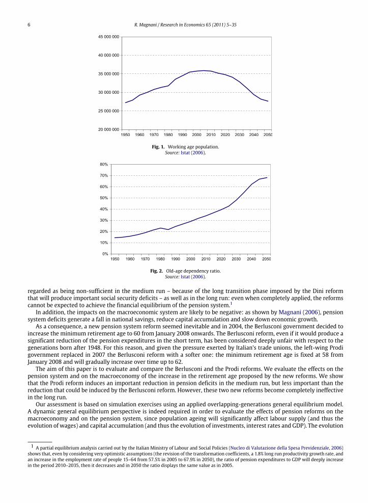
Industrialised countries will know a phase of significant demographic changes over the next 50 years. The increase inlife expectancy, the reduction of fertility rates and, most of all, the baby-boom produced during the Fifties and Sixties haveinduced a population ageing that will put the financing of the social security systems under considerable stress. Italiandemographics are quite representative of this largely European phenomenon. The demographic projections based on thecentral hypothesis presented by Istat (2006) show that the working age population – the number of people between 20 and64 – will drop by 23% between 2000 and 2050 (Fig. 1) and the old-age dependency ratio – the ratio of the number of peopleaged 65 and more to the working age population – will increase from 28.9% in 2000 to 68.1% in 2050 (Fig. 2).
To face this problem, most European countries have recently introduced pension system reforms. Even if Europeanpension systems remain essentially different, some similar measures have been introduced in order to reduce the pensionexpenditure burden: the indexation of pension benefits to prices, the increase in the retirement age and the increase of therole of private funding. However, the Pay-As-You-Go system is still largely the most important pillar of European pensionsystems.
During theNineties, two reforms of the pension systemwere implemented in Italy, the Amato reform (1992), and theDinireform (1995). Even if these reforms would induce a significant reduction in future pension benefits, they are unanimously
∗ Corresponding address: CEPII, 9, rue Georges Pitard, 75015 Paris, France.E-mail addresses: [email protected], [email protected].
1090-9443/$ – see front matter© 2010 Published by Elsevier Ltd on behalf of University of Venice.doi:10.1016/j.rie.2010.02.001
6 R. Magnani / Research in Economics 65 (2011) 5–35
Fig. 1. Working age population.Source: Istat (2006).
Fig. 2. Old-age dependency ratio.Source: Istat (2006).
regarded as being non-sufficient in the medium run – because of the long transition phase imposed by the Dini reformthat will produce important social security deficits – as well as in the long run: even when completely applied, the reformscannot be expected to achieve the financial equilibrium of the pension system.1
In addition, the impacts on the macroeconomic system are likely to be negative: as shown by Magnani (2006), pensionsystem deficits generate a fall in national savings, reduce capital accumulation and slow down economic growth.
As a consequence, a new pension system reform seemed inevitable and in 2004, the Berlusconi government decided toincrease the minimum retirement age to 60 from January 2008 onwards. The Berlusconi reform, even if it would produce asignificant reduction of the pension expenditures in the short term, has been considered deeply unfair with respect to thegenerations born after 1948. For this reason, and given the pressure exerted by Italian’s trade unions, the left-wing Prodigovernment replaced in 2007 the Berlusconi reform with a softer one: the minimum retirement age is fixed at 58 fromJanuary 2008 and will gradually increase over time up to 62.
The aim of this paper is to evaluate and compare the Berlusconi and the Prodi reforms. We evaluate the effects on thepension system and on the macroeconomy of the increase in the retirement age proposed by the new reforms. We showthat the Prodi reform induces an important reduction in pension deficits in the medium run, but less important than thereduction that could be induced by the Berlusconi reform. However, these two new reforms become completely ineffectivein the long run.
Our assessment is based on simulation exercises using an applied overlapping-generations general equilibrium model.A dynamic general equilibrium perspective is indeed required in order to evaluate the effects of pension reforms on themacroeconomy and on the pension system, since population ageing will significantly affect labour supply (and thus theevolution of wages) and capital accumulation (and thus the evolution of investments, interest rates and GDP). The evolution
1 A partial equilibrium analysis carried out by the Italian Ministry of Labour and Social Policies (Nucleo di Valutazione della Spesa Previdenziale, 2006)shows that, even by considering very optimistic assumptions (the revision of the transformation coefficients, a 1.8% long run productivity growth rate, andan increase in the employment rate of people 15–64 from 57.5% in 2005 to 67.9% in 2050), the ratio of pension expenditures to GDP will deeply increasein the period 2010–2035, then it decreases and in 2050 the ratio displays the same value as in 2005.

R. Magnani / Research in Economics 65 (2011) 5–35 7
of wages directly affects the evolution of social security contributions, whereas the evolution of GDP growth rates, with theapplication of the Dini reform, affects the evolution of pension benefits.
The model used in this paper is of the type pioneered by Auerbach and Kotlikoff (1987), though with significantdifferences: we introduce mortality, immigration, human capital accumulation, and endogenous growth. The introductionof mortality and immigration makes it possible to accurately reproduce the demographic projections and to simulate theeffects of changes in immigration flows. The introduction of human capital makes it possible to introduce a mechanismof endogenous growth based on the average level of knowledge present in the economy à la Lucas (1988). Human capitalaccumulation results from explicit decisions made by young people to invest time in education.
An important aspect related to population ageing is the effects of demographic change and pension reforms on educationdecisions and consequently on economic growth.2 Indeed, relative factor prices are likely to vary significantly in the nextdecades hence affecting the decision to invest or not in human capital. One can expect that the impact of population ageingon human capital formationwill be positive, since ageingwould boost wages and reduce interest rates, and that the increasein retirement age would encourage individuals to devote more time to schooling. The positive impact on economic growthcould be important3 and, as a consequence, produce positive effects on the financial situation of the pension system.
Our model treats Italy as a closed economy. The degree of the financial openness is a very important aspect (see Börsh-Supan et al. (2006); Agliettaet al. (2007), and Chateau et al. (2008)) since it affects the determination of the interest ratethat influences the evolution of the public debt, the evolution of capital accumulation, the economic growth, and so on.The choice to not consider Italy as an open economy is related to the fact that all developed countries are faced (even withdifferent degrees) to an important ageing phenomenon that will deeply affect the world interest rate. So, we think that anopen economy scenario, which implies that the interest rate is fixed at a constant world level, is not a plausible assumptionin our ageing context.
The paper is organised as follows: in the next section, we describe the characteristics of the Italian pension system andthe reforms recently introduced. In Sections 3 and 4, we describe the structure of the OLGmodel and its calibration. Section 5presents the simulation results concerning the Berlusconi and the Prodi reforms. Section 6 presents some sensitivity analysisconcerning the immigration and the value of pension benefits. We draw our conclusions in the last section.
2. The Italian pension system
The Italian pension system is almost entirely composed of a compulsory public Pay-As-You-Go system. An importantanomaly of the Italian pension system is that there is no clear separation between the pension system in its strict senseand the system of social aids in which benefits are not related to contributions. In particular, the Italian pension systemincludes pensions related to work (old-age pensions, disability pensions, pensions paid in the case of occupational diseasesand industrial injuries), and other pensions (survival pensions and welfare benefits for people aged 65 and more lackingadequate means of support). In particular, in 20054:– IVS pensions, including old-age pensions, pensions to survivors and disability benefits, accounted for 13.64% of GDPwith
18.383 millions pensions paid. The average pension benefit was 10557 euros.– Pensions paid in the case of occupational diseases and industrial injuries accounted for 0.30% of GDP with one million
pensions paid. The average pension benefit was 4132 euros.– Social assistance pensions (for people aged 65 and more lacking adequate means of support) accounted for 1.16% of GDP
with 3.841 millions pensions paid. The average pension benefit was 4306 euros.– Total pensions then accounted for 15.10% of GDP with 23.257 millions pensions paid. The average pension benefit was
9239 euros.
During the Nineties two reforms were introduced in order to reduce future total pension expenditures and to harmonisethe different pension regimes5: the Amato reform in 1992 and the Dini reform in 1995.
The most important innovations of the Amato reform (Law 421/1992) were (i) the indexation of pension benefits oninflation, and not on real wages; (ii) the increase of the age requirement to be entitled to an old-age pension from 60 formen and 55 for women with at least 15 years of contributions to 65 for men and 60 for women with at least 20 years ofcontributions.
The Dini reform (Law 335/1995) introduced the following rules for the computation of the pension benefits:– For people who started working after 1995, the pension benefits are computed according to a new rule: the contribution
based method. In this case, the contributions paid during the whole working life are virtually capitalised at the average
2 Other OLG models including an endogenous growth mechanism based on human capital are provided by Fougère and Mérette (1999), Sadahiro andShimasawa (2003) and Bouzahzaha et al. (2002).3 Barro (2001) estimates that an additional year of schooling by people aged 25 and more induces an increase in the economic growth rate of 0.44% per
year.4 Istat (2007a), Statistiche della previdenza e dell’assistenza sociale. I trattamenti pensionistici. Anno 2005.5 Until 1992 the Italian pension system was characterised by a very large number of funds and schemes, in which contributions and benefit rules varied
according to the sector (private or public sector, or self-employment). The harmonisation process of the different pension regimes, in particular concerningpublic and private employees, was accelerated by the Law 449/1997.
8 R. Magnani / Research in Economics 65 (2011) 5–35
rate of growth of nominal GDP; the value of the pension is equal to the capitalised value of the contributions multipliedby a transformation coefficient depending on the retirement age.
– For people who hadmore than 18 years of contributions in 1995, the pension benefits remain computed according to theearning based method, i.e. on the basis of the average of the labour incomes earned during the 10 last years for salariedworkers and the 15 last years for self-employed workers.
– For people who in 1995 had less than 18 years of contributions, the pension benefits are computed according to the pro-rata method. In this case, the pension benefits are given by a weighted average of the pension computed with the earningbased method and the contribution based method.
With the Dini reform, the eligibility requirements to be entitled to a seniority pensionwere set as follows:
– For salaried workers aged more than 57, 35 years of contributions are required;– For self-employed workers, 40 years of contributions are required; and it is reduced to 35 years of contributions if the
person is aged more than 58.
Workers can thus decide to retire at 57, with at least 35 years of contributions. The main goal of the Dini reform wasto penalise early retirement. In fact, with the contribution based method, if an individual works less, the value of pensionbenefits will be lower since he/she accumulates a lower amount of contributions and the transformation coefficient appliedwill also be lower.
In 2004, the Berlusconi government introduced a new reform (Law 243/2004) that increased the minimum retirementage. According to this reform, the eligibility requirements would become 40 years of contributions or 35 years ofcontributions at the age of 60 for salaried workers and 61 for self-employed workers starting from 2008. The minimumretirement age would be increased by one year in 2010 and by another year in 2014.
The Berlusconi reform was replaced by the one introduced by the Prodi government in 2007 (Law 247/2007). Withthe new reform, the increase of the minimum retirement age is more gradual: in 2008, the minimum retirement age forsalaried workers is 58 with at least 35 years of contributions. From 2009 onwards, the eligibility requirements are relatedto the sum of the retirement age and the number of years of contributions. In 2009, salaried workers aged no less then 59can retire if the sum is equal to 95. In 2011, salaried workers aged no less then 60 can retire if the sum is equal to 96. From2013 onwards, salaried workers aged no less than 61 can retire if the sum is equal to 97. For self-employed workers, theminimum retirement age is given by the minimum retirement age for salaried workers plus one year.
The reforms introduced until now harmonised the pension schemes for public and private salaried workers. In contrast,the rules applied to self-employed workers remain different, not only in terms of the eligibility requirements, but also interms of social contribution rates. For instance, the contribution rate of salaried workers in the public and private sectors isequal to 33%, while for self-employed workers it is quite lower and equal to 20%.
Finally, the Amato and theDini reforms have introduced and improved the legislation on supplementary funded schemes.Nevertheless, the number of workers enrolled in private pension funds remains very low.
3. The model
3.1. General characteristics
Themodel presented in this paper is an applied overlapping-generationsmodel of the type Auerbach and Kotlikoff (1987)with endogenous growth and immigration. We consider 15 age groups, indicated by g = 1, . . . , 15, that coexist at eachperiod t . The first age group considered is 20–24, the last one is 90–94. Each period consists of 5 years and all the variablesare supposed to be constant during each period.
For each age group, individuals are characterised by their origin and the professional status. Concerning the origin, wedistinguish two groups, indicated by z: those born in Italy (nat) and immigrants (imm).6 Concerning the professional status,we distinguish two groups, indicated by prof , the salaried workers (empl) and the self-employed workers (self ).
We assume the existence of a representative agent of people born in Italy and a representative agent of immigrants(intra-generation’s heterogeneity). We also assume that agents have perfect foresight and there is no liquidity constraint.
At the end of each period, people belonging to the last age group (g = 15) die, a fraction of people belonging to the otherclasses dies, and a new generation enters the active population.
Individuals maximise an intertemporal utility function subject to an intertemporal budget constraint. Immigrants andpeople born in Italy have the same structure of preferences. They decide the intertemporal profile of consumption and leisureas well as the value of the voluntary bequests that will be left at the end of the last period of life. On the other hand, onlypeople born in Italy decide the fraction of time to devote to studying. This decision allows the individual to constitute a stockof human capital that affects his/her productivity level and then his/her future earning profile. We introduce an endogenous
6 We assume that immigration only concerns the age group 30–34. This assumption, that allows us an important simplification of the model, is justifiedby the fact that data concerning resident permits (Istat, 2004) are normally distributed with a peak for the age group 30–34. In any case, the introductioninto the model of immigration at different age does not significantly change the results.
R. Magnani / Research in Economics 65 (2011) 5–35 9
growthmechanism à la Lucas (1988)where the productivity growth rate is related to the average level of knowledge presentin the economy.
Intra-generation’s heterogeneity is given by the assumption that immigrants differ from people born in Italy by a lowerlevel of productivity and that they enter Italy with no capital. On the other hand, the children of immigrants are consideredidentical to the children of people born in Italy. Consequently, they decide the fraction of time to devote to studying andthey display the same productivity as the children of natives.
Peoplewho die in the last period of life (95 years old) decide to leave bequests to the other generations, on the basis of themaximisation of their utility function. These voluntary bequests are uniformly distributed among the other generations. Onthe other hand, the presence of involuntary bequests is avoided by introducing an insurance mechanism à la Yaari (1965).
Concerning the production side of the model, in our economy, only one good is produced by using labour and capital inorder to maximise profits and given the following Cobb–Douglas technology:
Yt = Kαt · L1−α
t (1)
where Yt represents the production level of the period, Kt the physical capital demand, and Lt the per unit of effective labourdemand. Labour and capital markets are assumed to be perfectly competitive. This implies that real wages and real interestrates adjust to equilibrate aggregate demand and aggregate supply.
Aggregate capital supply depends on the individual’s capital accumulation, while aggregate labour supply depends onthe demographic evolution and on the individual’s labour market choices. Labour is supplied by salaried workers and self-employed workers aged between 20 and 64. Labour supply is endogenous for people aged between 20 and 54. In particular,people belonging to the first age group (20–24 years old) decide the fraction of time to devote to the accumulation of humancapital and to work. The following age groups, until the class 50–54, decide the fraction of time to devote to working and toleisure.With regard to the two last age groupswhowork (55–59 and 60–64), the fraction of peoplewhowork is exogenouslyfixed, according to the 2005 data. This permits us to simulate the impact of an exogenous increase in the retirement age.
The distinction between (private and public) salaried workers and self-employed is introduced into the model becausethe social contribution rates, the computation rule of pension benefits and the eligibility criteria are different. Thus, it isimportant to distinguish individuals according to their professional status in order to model the pension system accurately.We do not explicitly model the choice of the professional status, and we simply assume that the proportion of salariedworkers and self-employed workers is the same for each group and remains constant over time.
In the next paragraphs, we describe in more detail the demographic aspects of the model (i.e. the procedure adopted inorder to reproduce thedemographic projections by selecting the fertility rates, the survival probabilities and the immigrationflows), the generations’ behaviour and the government budget, focusing in particular on the pension system.
3.2. The demographic evolution
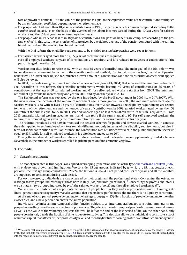
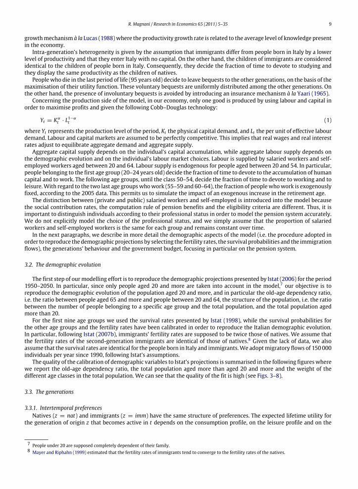
The first step of ourmodelling effort is to reproduce the demographic projections presented by Istat (2006) for the period1950–2050. In particular, since only people aged 20 and more are taken into account in the model,7 our objective is toreproduce the demographic evolution of the population aged 20 and more, and in particular the old-age dependency ratio,i.e. the ratio between people aged 65 and more and people between 20 and 64, the structure of the population, i.e. the ratiobetween the number of people belonging to a specific age group and the total population, and the total population agedmore than 20.
For the first nine age groups we used the survival rates presented by Istat (1998), while the survival probabilities forthe other age groups and the fertility rates have been calibrated in order to reproduce the Italian demographic evolution.In particular, following Istat (2007b), immigrants’ fertility rates are supposed to be twice those of natives. We assume thatthe fertility rates of the second-generation immigrants are identical of those of natives.8 Given the lack of data, we alsoassume that the survival rates are identical for the people born in Italy and immigrants.We adoptmigratory flows of 150000individuals per year since 1990, following Istat’s assumptions.
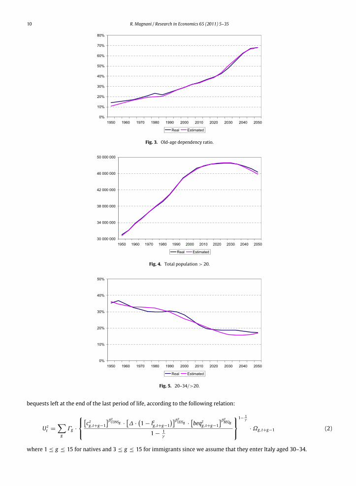
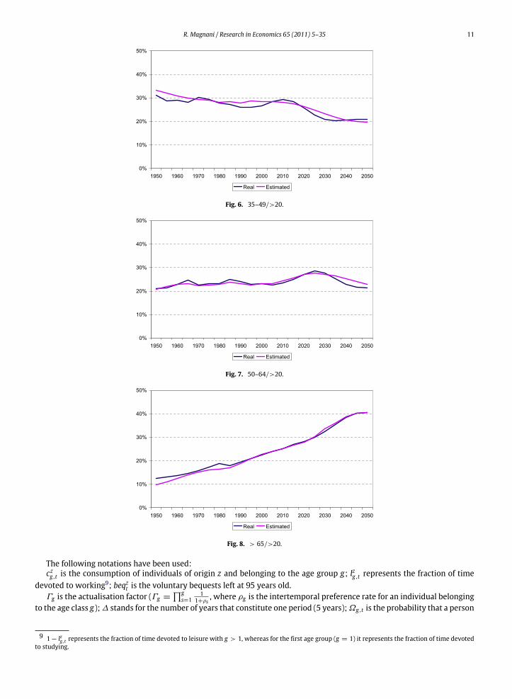
The quality of the calibration of demographic variables to Istat’s projections is summarised in the following figureswherewe report the old-age dependency ratio, the total population aged more than aged 20 and more and the weight of thedifferent age classes in the total population. We can see that the quality of the fit is high (see Figs. 3–8).
3.3. The generations
3.3.1. Intertemporal preferencesNatives (z = nat) and immigrants (z = imm) have the same structure of preferences. The expected lifetime utility for
the generation of origin z that becomes active in t depends on the consumption profile, on the leisure profile and on the
7 People under 20 are supposed completely dependent of their family.8 Mayer and Riphahn (1999) estimated that the fertility rates of immigrants tend to converge to the fertility rates of the natives.
10 R. Magnani / Research in Economics 65 (2011) 5–35
Fig. 3. Old-age dependency ratio.
Fig. 4. Total population > 20.
Fig. 5. 20–34/>20.
bequests left at the end of the last period of life, according to the following relation:
U zt =
−g
Γg ·
czg,t+g−1
βzCONSg ·
∆ ·
1 − lzg,t+g−1
βzLEISg ·
beqzg,t+g−1
βzBEQg
1 −1γ
1− 1
γ
· Ωg,t+g−1 (2)
where 1 ≤ g ≤ 15 for natives and 3 ≤ g ≤ 15 for immigrants since we assume that they enter Italy aged 30–34.
R. Magnani / Research in Economics 65 (2011) 5–35 11
Fig. 6. 35–49/>20.
Fig. 7. 50–64/>20.
Fig. 8. > 65/>20.
The following notations have been used:czg,t is the consumption of individuals of origin z and belonging to the age group g; lzg,t represents the fraction of time
devoted to working9; beqzt is the voluntary bequests left at 95 years old.Γg is the actualisation factor (Γg =
∏gs=1
11+ρs
, where ρg is the intertemporal preference rate for an individual belongingto the age class g);∆ stands for the number of years that constitute one period (5 years);Ωg,t is the probability that a person
9 1− lzg,t represents the fraction of time devoted to leisure with g > 1, whereas for the first age group (g = 1) it represents the fraction of time devotedto studying.
12 R. Magnani / Research in Economics 65 (2011) 5–35
that belongs to the age group g is alive in t; γ is the intertemporal elasticity, while the intra-temporal elasticity is assumedto be equal to 1.
βzCONSg , β
zLEISg and βz
BEQgmeasure respectively the intensity of the preference for consumption, for leisure and for bequests.
In particular:βzCONSg = 1, βz
LEISg = 0, βzBEQg
= 0 if g = 1βzCONSg = 1 − βz
LEISg , βzLEISg > 0, βz
BEQg= 0 if 2 ≤ g ≤ 7
βzCONSg = 1, βz
LEISg = 0, βzBEQg
= 0 if 8 ≤ g ≤ 14βzCONSg = 1 − βz
BEQg, βz
LEISg = 0, βzBEQg
> 0 if g = 15.
3.3.2. Individual productivity and human capital accumulationThe labour income for an individual of origin z, belonging to the age group g and working in the professional activity
prof , is given by the product between the wage per unit of effective labour (wt ) and the total productivity level specific tothe individual (Az
g,prof ,t ).In particular, the wage per unit of effective labour, identical for each individual, is endogenously determined in order to
guarantee the labour market equilibrium, see Eq. (23).The individual productivity level depends on five elements:
(i) The individual’s age, measured by EPg . This component exerts a standard quadratic form:
EPg = θ0 + θ1g + θ2g2 (3)
with 1 ≤ g ≤ 9 since only people in the first nine age groups work, and θ1 > 0, θ2 < 0.(ii) The individual’s education level, measured by HC z
g,t . The stock of human capital accumulated by natives (z = nat)belonging to the first age group (20–24) depends on the number of years devoted to studying according to the followingincreasing and concave relation:
HCnat1,t =
∆ ·
1 − lnat1,t
αHC (4)
where∆ ·
1 − lnat1,t
is the number of years devoted to studying and αHC > 0. Afterwards, the individual human
capital depreciates at a constant rate δHC :
HCnatg,t = (1 − δHC ) · HCnat
g−1,t−1.
Given that immigrants enter Italy aged 30–34, they are not concerned by the choice of the education level, then theirhuman capital stock (HC imm
g,t ) is considered exogenous.(iii) An externality component,measured byHt , related to the average level of knowledge present in the economy, indicated
by H t . This latter component is given by the weighted average of the stocks of human capital of each age class thatworks at the same period: H t =
∑z∑
g HCzg,t ·l
zg,t ·Pop
zg,t∑
z∑
g lzg,t ·Popzg,t
. Moreover, we introduce an endogenous growth mechanism à laLucas (1988) in the following way: the productivity growth rate (gHt ), which represents the steady state growth rate ofvariables in per capita terms, is endogenous and supposed to be related to the average level of knowledge as follows:
gHt =Ht+1 − Ht
Ht= χ · H
1αHCt (5)
where χ > 0. As no individual could influence, by his/her decision to study, the value of this index, this stands as apositive externality.
(iv) The individual’s professional status, measured by Ψprof , that represents the (exogenous and constant) difference inproductivity between salaried workers and self-employed workers.
(v) The individual’s origins, measured by θ z , that represents the difference in productivity between natives and immigrantsin the base year. However, note that the difference in productivity between natives and immigrants may change overtime since the human capital stock of natives is endogenous.
Finally, the individual’s total productivity (Azg,prof ,t ) is given by the product of the previous elements:
Azg,prof ,t = EPg · HC z
g,t · Ht · Ψprof · θ z . (6)
Given that the productivity difference between salaried workers and self-employed workers is assumed to be constantand that the individual choice between these two options is not modelled, we can define an average productivity, indicatedby Az
g,t . This element is computed as the average of Azg,prof ,t weighted by the proportion (assumed to be the same for each
age group and constant over time) of salaried workers and self-employed workers.
R. Magnani / Research in Economics 65 (2011) 5–35 13
3.3.3. Pension benefitsPension benefits are computed according to the rules introduced by the Amato and Dini reforms. In our analysis, we
consider three types of pensions, indicated by type: direct pensions (dir), disability benefits (dis) and pensions to survivors(surv). These pensions are paid to the retirees according to their professional status prof , i.e. to salaried workers (empl) andself-employed workers (self ). We begin with the description of the computation of direct pensions.
The value of direct pension benefits is computed in themodel by applying the earning based method for the pensions paiduntil 2015, the pro-rata method for the pensions paid between 2015 and 2030, and the contribution based method for thepensions paid from 2030.
First of all, it is necessary to distinguish pension benefits paid to individuals belonging to the age group 55–59 and toindividuals belonging to the age group 60–64. For the latter, only a fraction of people retires between 60 and 64, while thecomplement fraction retires during the previous period (55–59).
For the retirees belonging to the age group 55–59 (g = 8), pension benefits are computed in the following way:
– Earning based method (t < 2015): the annual pension benefit is computed on the basis of the average income earnedduring the last 10 years (the last two periods in our model) for salaried workers (empl) and during the last 15 years (thelast three periods in our model) for self-employed workers (self ):
Pensz8,empl,dir,t = nz8 · 0.02 ·
wt · Az
8,empl,t + wt−1 · Az7,empl,t−1
2
(7)
Pensz8,self ,dir,t = nz8 · 0.02 ·
wt · Az
8,self ,t + wt−1 · Az7,self ,t−1 + wt−2 · Az
6,self ,t−2
3
. (8)
The replacement ratio is then proportional to the number of years worked by the class 55–59, indicated by nz8.
– Contribution based method (t > 2030): the annual pension benefit for each professional status (salaried workers and self-employed) is computed bymultiplying the transformation coefficient β8 by the value of the contributions paid during thewhole working life and capitalised on the basis of the average GDP growth rate (gGDPt ):
Pensz8,prof ,dir,t = β8 ·
−g
τ c· wt+g−8 · Az
g,prof ,t+g−8 ·
t∏s=t+g−8
1 + gGDPs
(9)
with 1 ≤ g ≤ 8 for people born in Italy and 3 ≤ g ≤ 8 for immigrants.– Pro-rata method (2015 ≤ t ≤ 2030): the annual pension benefit is equal to a weighted average between the pension
benefit computed with the earning based method and the contribution based method, where the weight depends on thenumber of years worked before and after 1995.
For the retirees belonging to the age group 60–64 (g = 9), we have to consider that only a fraction (noted by λ) of theseindividuals retires between 60 and 64 and that the complement fraction (1− λ) retires during the previous period (55–59).On average, the pension benefit obtained by the representative individual aged 60–64 is computed in the following way:
– Earning based method (t < 2015): the annual pension benefit for salaried workers and self-employed workers is givenby:
Pensz9,empl,dir,t = λ ·
[nz9 · 0.02 ·
wt · Az
9,empl,t + wt−1 · Az8,empl,t−1
2
]+ (1 − λ) · Pensz8,empl,dir,t−1 (10)
Pensz9,self ,dir,t = λ ·
[nz9 · 0.02 ·
wt · Az
9,self ,t + wt−1 · Az8,self ,t−1 + wt−2 · Az
7,self ,t−2
3
]+ (1 − λ) · Pensz8,self ,dir,t−1. (11)
– Contribution based method (t > 2030):
Pensz9,prof ,dir,t = λ ·
β9 ·
−g
τ c· wt+g−9 · Az
g,prof ,t+g−9 ·
t∏s=t+g−9
1 + gGDPs
+ (1 − λ) · Pensz8,prof ,dir,t−1. (12)
– Pro-rata method (2015 ≤ t ≤ 2030): with regard to the fraction λ of individuals who retire between 60 and 64, pensionbenefits are given by a weighted average between the pension benefits computed with the earning based method andthe contribution based method, whereas the fraction (1 − λ) of workers who retire in the previous period, receivesPensz8,prof ,dir,t−1.
Concerning the indexation of pension benefits, from 1992 onwards, pension benefits are not indexed to real wages, butto prices, and therefore remain constant over time in real terms:
Penszg,prof ,dir,t+g−9 = Pensz9,prof ,dir,t (13)
with 10 ≤ g ≤ 15.
14 R. Magnani / Research in Economics 65 (2011) 5–35
The transformation coefficients β are defined by Law 335/1995 and vary according to the retirement age of theindividual: they lie between 4.72% for people who retire at 57 and 6.136% for people who retire at 65. According to Law335/1995, these coefficients must be updated every ten years according to the evolution of the life expectancy. In themodel, the transformation coefficients used in the model for the age groups 55–59 and 60–64 (respectively β8 and β9)are endogenously determined by considering the average retirement age within the two age groups.
Concerning disability benefits and pension benefits to survivors we assume that they are proportional to the directpension benefits. Disability benefits and pension benefits to survivors are then computed in the model by applying acoefficient that permits to reproduce the data concerning the average pension benefits (see below Tables 1a and 1b inSection 4.1).
3.3.4. Intertemporal budget constraintEach agent maximises his/her intertemporal utility function conditional on his/her intertemporal budget constraint. For
people who live until the last age group (95 years old), the end of life wealth is left as voluntary bequests. In the caseof premature death, in order to avoid the presence of involuntary bequests, we assume the existence of a life insurancesector which offers actuarially fair annuities, where the actuarial rate of interest exceeds the market rate of interest by theconditional mortality probability (Yaari, 1965).
The present value of the final wealth is given by the difference between the present value of future incomes and thepresent value of future consumption. In particular, incomes are given by net labour incomes, net pensions and inheritances.
Thus, for each period, the budget constraint for an individual of origin z and belonging to the age group g is as follows:
wealthzg+1,t+1 = [1 + (1 − τt) · rt ] · wealthz
g,t + (1 − ωg,t) · wealthzg+1,t+1 + (1 − τt − τ c) · wt · Az
g,t · lzg,t
+
−prof
−type
(1 − τt) · Penszg,prof ,type,t · npensg,prof ,type,t + inhzg · beqz15,t ·
Popz15,tPopzg,t
− czg,t (14)
where:wealthz
g,t is the wealth owned by individuals of origin z and belonging to the age group g;rt is the interest rate;τt is the income tax rate;τ c is the social contribution rate (computed as the average between the social contribution rate applied to salaried
workers and to self-employed workers);npensg,prof ,type,t is the fraction of individuals belonging to the age group g who receives pension benefits, according to the
professional status and the type of benefits10;ωg,t is the survival probability for an individual belonging to the class age g in t;inhz
g is a parameter computed in order to distribute the voluntary bequests uniformly among the generations.
3.3.5. Optimal individual choicesBy maximising utility, each individual chooses simultaneously the fraction of time to devote to schooling, his/her
intertemporal profile of leisure and consumption, and the amount of bequest to leave if he/she survives until 95 years old.The first order conditions are the following:
(i) Decision of studying, which only concerns natives (z = nat) belonging to the age group g = 1:1 − τt − τ c
·wt · Anat
1,t
∆
=
9−g=1
Rt+g−1 ·1 − τt+g−1 − τ c
· wt+g−1 · lnatg,t+g−1 ·∂Anat
g,t+g−1
∂∆ ·
1 − lnat1,t
· Ωg,t+g−1 (15)
where Rt represents the discount factor, with Rt+g−1 =∏t+g−1
s=t+11
1+(1−τs)·rs.
This conditionmeans that if an individual decides at t to study onemore year,11 he gives up to one year of wage (the LHS)that, at the optimum, must be equal to the expected present value of all additional incomes earned thanks to the increasein the productivity related to human capital (the RHS).
Ceteris paribus, individuals decide to devote more time to human capital accumulation when future wages are expectedto increase or future interest rates are expected to decrease, and when the survival probabilities increase.
10 The parameter npensg,prof ,type,t is related to lzg,t . In fact lzg,t represents not only the fraction of time devoted to working by the representative agent, butalso the fraction of individuals that belong to an age class who work.11 Note that ∆ ·
1 − lnat1,t
indicates the number of years devoted to studying by people belonging to the first age group.
R. Magnani / Research in Economics 65 (2011) 5–35 15
(ii) Decision concerning the leisure (for age groups 2 ≤ g ≤ 7):
1 − lzg,t =
βzLEISg
1 − βzLEISg
·czg,t
(1 − τt − τ c) · wt · Azg,t
. (16)
Ceteris paribus, an increase in the net wage induces an increase in the individual’s labour supply.(iii) Intertemporal profile of consumption:
czg+1,t+1
czg,t=
[1 + (1 − τt+1) · rt+1
1 + ρg+1
]γ
·
1 − βz
LEISg+1
1 − βzLEISg
γ
×
(1 − τt+1 − τ c) · Az
g+1,t+1 · wt+1βz
LEISg+1(1 − τt − τ c) · Ag,t · wt
βzLEISg
βzLEISg
1−βzLEISg
βzLEISg
βzLEISg+1
1−βzLEISg+1
βzLEISg+1
1−γ
. (17)
(iv) Voluntary bequests (for the age group g = 15):
beqz15,t+14 =βzBEQ15
1 − βzBEQ15
· cz15,t+14. (18)
The individual’s optimal bequests are then proportional to his/her consumption in the last period of life.
3.4. The government
3.4.1. The pension systemThe Italian pension system is a Pay-As-You-Go system in which workers pay social security contributions (33% of wages
for the public and private salaried workers and 20% of wages for self-employed workers) and the pension benefits arecomputed according to the rules introduced by the Amato and Dini reforms as described in Section 3.3.3.
The deficit of the pension system is computed as follows:
DefPSt =
−z
−g
−prof
−type
Popzg,t · Penszg,prof ,type,t · npensg,prof ,type,t −
−z
−g
Popzg,t · τ c· wt · Az
g,t · lzg,t . (19)
3.4.2. Public expenditures and government savingsIn the model, we consider three types of public expenditures: expenditures on the education of young people aged from
5 to 24, health care expenditures, and others public expenditures (public defence, public administration, etc.).Public spending on education (Gedut ) is assumed to be proportional to the number of people attending school, while
health care expenditure (Gmedt ) is proportional to the number of people agedmore than 60.We also assume that the averageexpenditure per student and the average health expenditure per old person vary over time according to the evolution of theGDP. Concerning the other public expenditures (Gt ), we assume they grow at the same rate as the GDP.
Government savings (Sgovt ) are given by the difference between revenues (taxes on labour and capital incomes and onpension benefits) and expenditures (expenditures on education, on health and public expenditures, the deficit of the pensionsystem, and the interests paid on the public debt):
Sgovt =
−z
−g
Popzg,t · τt ·
wt · Az
g,t · lzg,t + rt · wealthzg,t +
−prof
−type
Penszg,prof ,type,t · npensg,prof ,type,t
−Gedut + Gmedt + Gt + DefPSt + rt · Bt
. (20)
We fix the ratio of the public debt (Bt ) to GDP and we determine, for each period, the income tax rate (τt ) that permitsto respect this budget constraint.
3.5. Equilibrium conditions
There are three markets in the model: the market of goods and services, the capital market and the labour market. Thesemarkets are supposed to be perfectly competitive, so prices adjust in order to guarantee themarket clearing. The equilibrium
16 R. Magnani / Research in Economics 65 (2011) 5–35
conditions are the following:
Yt =
−z
−g
Popzg,t · czg,t + Gedut + Gmedt + Gt + It (21)
Kt + Bt =
−z
−g
Popzg,t · wealthzg,t (22)
Lt =
−z
−g
Popzg,t · lzg,t · Azg,t . (23)
Eq. (21) represents the equilibrium in the market of goods and services: production must be equal to aggregate demand,given by the private and public consumption and by the investments.
Eq. (22) represents the equilibrium in the capital market. In our model we consider two assets, physical capital andgovernment bonds, that are supposed perfectly substitutes, so their remuneration must be the same. The equilibriumcondition is that assets demanded by firms and government (LHS) should equal the aggregate household wealth, wherewealthz
g,t is the individual wealth depending on his/her life-cycle saving profile defined in Eq. (14).Eq. (23) indicates that the total labour supply expressed in per unit of effective labour (RHS) is entirely used in the
production activity.One of the previous equations is redundant by the Walras Law and we consider the domestic good as the numeraire.
3.6. Dynamics of the economy
The dynamics of the economy concern the evolution of labour supply, capital, government bonds and productivity. Theevolution of labour supply depends on the individual labour choices (i.e. the choices concerning the fraction of time devotedto schooling and leisure) and on the demographic evolution (i.e. the evolution of fertility rates, survival probabilities andimmigration flows). The labour productivity evolves over time according to the endogenous growth mechanism describedin Eq. (5). Finally, the evolution of the capital stock depends on investments and on capital depreciation, while public debtdepends on government savings, as follows:
Kt+1 = Kt · (1 − δ) + It (24)Bt+1 = Bt − Sgovt . (25)
4. Calibration of the model
The aim of our calibration is two-fold: reproduce the 2005 Italian macroeconomic data (in particular, the value of theGDP, the ratio between aggregate consumption and GDP, the ratio between investments and GDP, and the ratio betweenpublic expenditures and GDP) and replicate the most important ingredients of the pension system (the ratio of the numberof retirees to the number ofworkers, the average pension benefits for each type of pensions, and the ratio of the total pensionexpenditure to GDP).
4.1. The calibration of the pension system
Given that our objective is to evaluate the impacts of pension reforms in the context of population ageing, we focus onthe IVS pensions (including old-age direct pensions, pensions to survivors and disability benefits). IVS pensions account for13.64% of GDP in 2005 (Istat, 2007a).
However, in our analysis, we do not consider:
– IVS pensions paid by private institutions that account for 0.16% of GDP.– Supplementary pensions12 that account for 0.33% of GDP.– Pensions paid to people aged less than 55.
Then, the pension system analysed in our paper accounts for 12.89% of GDP in 2005.In particular, pensions to public and private salariedworkers account for 10.50% of GDP, while pensions to self-employed
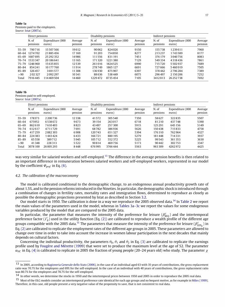
account for 2.39%. Direct pensions account for 9.87% of GDP, disability benefits for 0.88% and pensions to survivors for 2.14%.Tables 1a and 1b present the main characteristics of the pension system analysed in our paper. Data show that, concerningdirect pensions, the average pension benefits earned by self-employed are 40% lower than those earned by salariedworkers.This relevant difference is not related to a different calculation rule of pensions: in fact, in 2005, the gross replacement ratio
12 Supplementary pension systems, recently introduced in the Italian system, are mostly funded and voluntary. They include closed-end funds andcollective pension funds.
R. Magnani / Research in Economics 65 (2011) 5–35 17
Table 1aPensions paid to the employees.Source: Istat (2007a).
Direct pensions Disability pensions Indirect pensionsN. ofpensions
Expenditure (000euros)
Averagepension
N. ofpensions
Expenditure (000euros)
Averagepension
N. ofpensions
Expenditure (000euros)
Averagepension
55–59 790716 15507566 19612 90062 824026 9150 155738 1239611 796060–64 1274702 21885456 17169 91203 754850 8277 213237 1743589 817765–69 1687695 25292352 14986 111556 831191 7451 376179 3040756 808370–74 1533347 20186641 13165 171320 1221380 7129 549334 4318436 786175–79 1246960 15635855 12539 261016 1824525 6990 715720 5502937 768980–84 854241 10177760 11914 278749 1865127 6691 727666 5460919 750585–89 326457 3691577 11308 136930 875907 6397 378442 2796284 7389>90 202327 2092297 10341 88636 538449 6075 296497 2150206 7252Total 7916445 114469504 14460 1229472 8735454 7105 3412813 26252738 7692
Table 1bPensions paid to self-employed.Source: Istat (2007a).
Direct pensions Disability pensions Indirect pensionsN. ofpensions
Expenditure (000euros)
Averagepension
N. ofpensions
Expenditure (000euros)
Averagepension
N. ofpensions
Expenditure (000euros)
Averagepension
55–59 178373 2200736 12338 41572 305540 7350 58627 322835 550760–64 675952 6538672 9673 39154 263017 6718 81210 437748 539065–69 862610 7610403 8823 43497 257300 5915 125291 645156 514970–74 612617 4711729 7691 68782 386936 5626 150438 715833 475875–79 417259 2882303 6908 120743 651327 5394 176310 762964 432780–84 224383 1443424 6433 166721 880195 5279 181448 714331 393785–89 65558 389712 5945 105712 552372 5225 99543 361353 3630>90 41348 228313 5522 90814 469756 5173 90442 302753 3347Total 3078100 26005293 8448 676995 3766444 5563 963309 4262972 4425
was very similar for salaried workers and self-employed.13 The difference in the average pension benefits is then related toan important difference in remuneration between salaried workers and self-employed workers, represented in our modelby the coefficient Ψprof in Eq. (6).
4.2. The calibration of the macroeconomy
The model is calibrated conditional to the demographic change, to an endogenous annual productivity growth rate ofabout 1.5%, and to thepension reforms introduced in theNineties. In particular, the demographic shock is introduced througha combination of changes in fertility rates, mortality rates and immigration flows, determined to reproduce as closely aspossible the demographic projections presented by Istat as described in Section 3.2.
Our model starts in 1950. The calibration is done in a way we reproduce the 2005 observed data.14 In Table 2 we reportthe main values of the parameters used in the model, whereas in Tables 3a–3c we report the values for some endogenousvariables produced by the model that are compared to the 2005 data.
In particular, the parameter that measures the intensity of the preference for leisure (βzBEQ ) and the intertemporal
preference factor (Γg ) used in the utility function (Eq. (2)) are calibrated to reproduce a wealth profile of the different agegroups compatible with the 2005 data.15 The parameters that measure the intensity of the preference for leisure (βz
LEISg ) inEq. (2) are calibrated to replicate the employment rates of the different age groups in 2005. These parameters are allowed tochange over time in order to take into account the increase in women labour participation in the next decades that mainlydepends on cultural factors.
Concerning the individual productivity, the parameters θ0, θ1 and θ2 in Eq. (3) are calibrated to replicate the earningsprofile used by Fougère and Mérette (1999) that were set to produce the maximum level at the age of 52. The parameterαHC in Eq. (4) is calibrated to replicate in 2005 the fraction of young people (20–24 years old) who study. The parameter χ
13 In 2005, according to Ragioneria Generale dello Stato (2006), in the case of an individual aged 63 with 35 years of contributions, the gross replacementratio was 70.7% for the employees and 69% for the self-employed. In the case of an individual with 40 years of contributions, the gross replacement ratiowas 80.7% for the employees and 78.7% for the self-employed.14 In other words, we determine the stocks in 1950 and the intertemporal prices between 1950 and 2005 in order to reproduce the 2005 real data.15 Most of the OLGmodels consider an intertemporal preference rate identical for each age groups and no bequest motive, as for example inMiles (1999).Therefore, in this case, old people present a very negative value of the propensity to save, that is not consistent to real data.
18 R. Magnani / Research in Economics 65 (2011) 5–35
Table 2Some parameters used in the model.
Households
θ0 0.675Productivity related to the age θ1 0.350
θ2 −0.025Productivity related to the education αHC 0.339Productivity related to the average level of knowledge χ 0.089Intertemporal elasticity of substitution γ 0.75
βLEIS2 0.597βLEIS3 0.713
Index of preference for leisure βLEIS4 0.744βLEIS5 0.754βLEIS6 0.761βLEIS7 0.735
Index of preference for bequests βBEQ 1.098
Firms
Annual depreciation rate of physical capital δ 5%Capital remuneration in the added value α 0.412
Government
Contribution rate applied to salaried workers 33%Contribution rate applied to self-employed workers 20%Average contribution rate τ c 23.3%Public debt/GDP 106.4%Total public expenditure/GDP 20.4%
Table 3aVariables concerning the macroeconomy, year 2005.
Generated values of main endogenous variables compared with real data
Simulated value Real data
GDP (in milliards of euros) 1423.022 1423.049Consumption/GDP 59.00% 58.63%Investments/GDP 20.50% 20.42%Gedu/GDP 4.58% 4.62%Gmed/GDP 6.95% 6.93%G/GDP 8.96% 8.87%Income tax rate 14.8%K/GDP 2.65
in Eq. (5) is calibrated to obtain a productivity growth rate in 2005 close to 1.5%. The parameter θ z is chosen such that thetotal productivity of immigrants is lower by 13% of the total productivity of natives.16
Both the calibration and simulations were made by using numerical algorithms provided by GAMS (General AlgebraicModelling System).
5. Effects of the recent reforms: Berlusconi and Prodi reforms
We now use the model to simulate and compare the pension reforms recently introduced: the Berlusconi reform (2004)and the Prodi reform (2007). Whereas with the Dini reform workers can decide to retire between 57 and 65, the two newreforms increase the minimum retirement age.
In particular, with the Berlusconi reform, the minimum retirement age is increased to:
– 60 (61 for self-employed workers), after January 2008.– 61 (62 for self-employed workers), after 2010.– 62 (63 for self-employed workers), after 2014.
16 Storesletten (2000) finds, for the United States, that the productivity of immigrants aged 37 is lower by 13% with respect to that of natives. In ourcase, this assumption implies that immigrants have a level of productivity related to education lower by 13% compared to natives. In fact, we can supposethat an immigrant and a native, with the same age, have the same productivity related to the experience (EP) and that they profit in the same way ofthe knowledge present in the economy (H). By considering Eq. (4), this assumption implies that immigrants have a stock of human capital lower by 10%relatively to natives.
R. Magnani / Research in Economics 65 (2011) 5–35 19
Table 3bVariables concerning the labour market, year 2005.
Simulated value Real data
20–24 41.16% 41.11%25–29 63.24% 63.26%30–34 74.06% 74.36%35–39 76.01% 76.22%
Employment rates 40–44 76.23% 76.40%45–49 74.03% 74.06%50–54 66.71% 66.87%55–59 43.07% 43.07%60–64 17.99% 17.99%
National employment rate 61.29% 61.48%Employment rate for natives 60.76% 61.12%Employment rate for immigrants 69.85% 70.05%Retirees/Workers 0.784 0.786
Table 3cPension system expenditures with respect to GDP, year 2005.
Simulated value Real data
All pensions 12.97% 12.89%
Direct pensions 8.09% 8.04%Salaried workers disability benefits 0.61% 0.61%
Indirect pensions 1.82% 1.84%
Direct pensions 1.89% 1.83%Self-employed workers disability benefits 0.26% 0.26%
Indirect pensions 0.30% 0.30%
The Berlusconi reform was replaced in 2007 by a new reform introduced by the Prodi government where the increase ofthe minimum retirement age is more gradual:
– 58 (59 for self-employed workers) with at least 35 years of contributions, after 2008.– 59 (60 for self-employed workers) with at least 36 years of contributions, or 60 (61 for self-employed workers) with at
least 35 years of contributions, after 2009.– 60 (61 for self-employed workers) with at least 36 years of contributions, or 61 (62 for self-employed workers) with at
least 35 years of contributions, after 2011.– 61 (62 for self-employed workers) with at least 36 years of contributions, or 62 (63 for self-employed workers) with at
least 35 years of contributions, after 2013.
These two reforms are compared with our base scenario in which the increase in the retirement age is not taken intoaccount.
5.1. Macroeconomic impacts
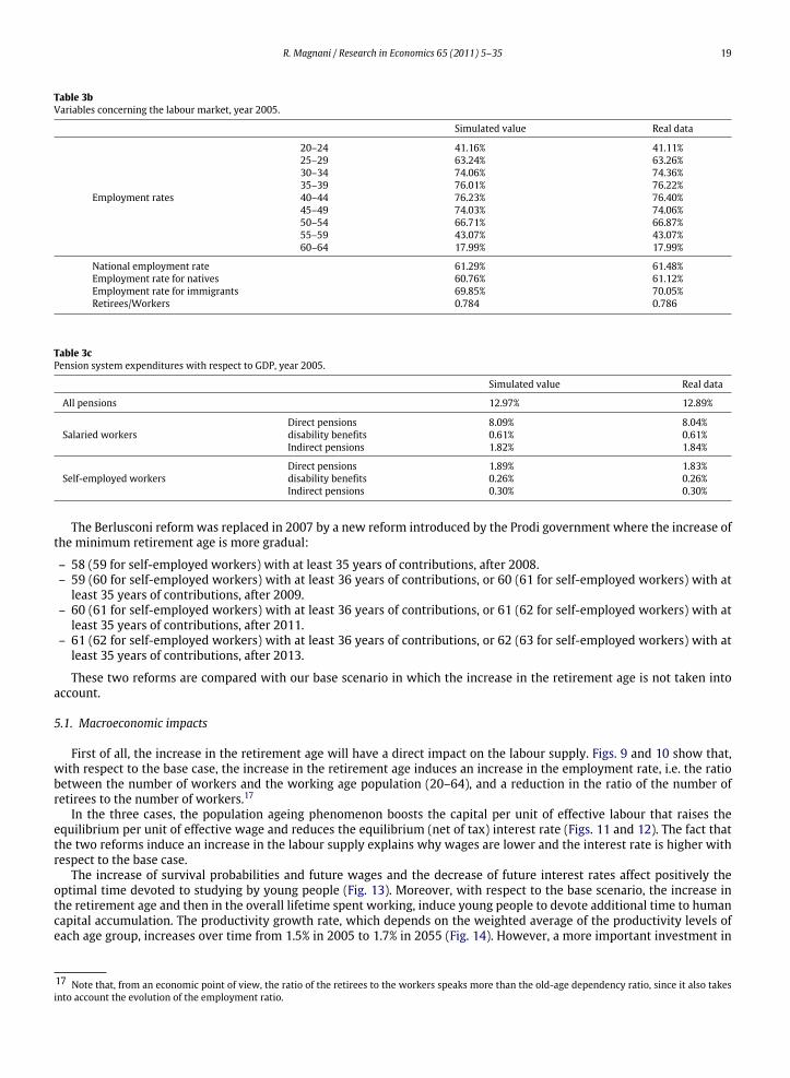
First of all, the increase in the retirement age will have a direct impact on the labour supply. Figs. 9 and 10 show that,with respect to the base case, the increase in the retirement age induces an increase in the employment rate, i.e. the ratiobetween the number of workers and the working age population (20–64), and a reduction in the ratio of the number ofretirees to the number of workers.17
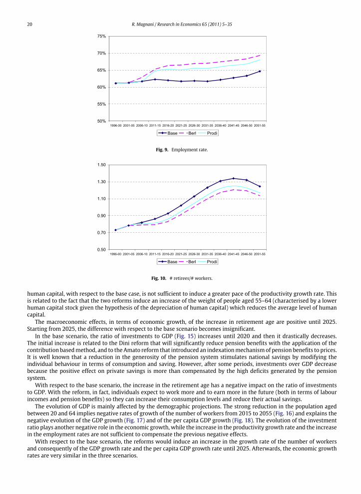
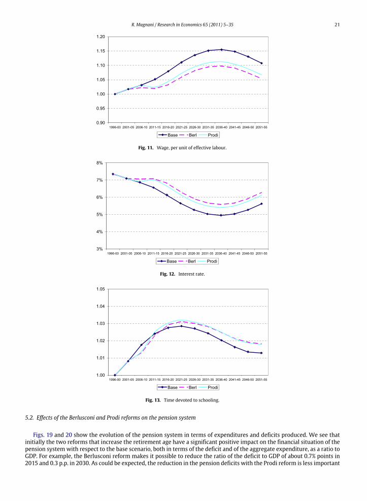
In the three cases, the population ageing phenomenon boosts the capital per unit of effective labour that raises theequilibrium per unit of effective wage and reduces the equilibrium (net of tax) interest rate (Figs. 11 and 12). The fact thatthe two reforms induce an increase in the labour supply explains why wages are lower and the interest rate is higher withrespect to the base case.
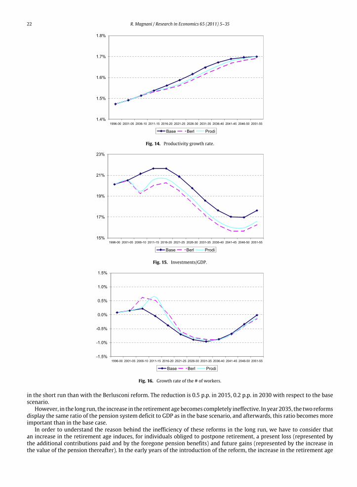
The increase of survival probabilities and future wages and the decrease of future interest rates affect positively theoptimal time devoted to studying by young people (Fig. 13). Moreover, with respect to the base scenario, the increase inthe retirement age and then in the overall lifetime spent working, induce young people to devote additional time to humancapital accumulation. The productivity growth rate, which depends on the weighted average of the productivity levels ofeach age group, increases over time from 1.5% in 2005 to 1.7% in 2055 (Fig. 14). However, a more important investment in
17 Note that, from an economic point of view, the ratio of the retirees to the workers speaks more than the old-age dependency ratio, since it also takesinto account the evolution of the employment ratio.
20 R. Magnani / Research in Economics 65 (2011) 5–35
Fig. 9. Employment rate.
Fig. 10. # retirees/# workers.
human capital, with respect to the base case, is not sufficient to induce a greater pace of the productivity growth rate. Thisis related to the fact that the two reforms induce an increase of the weight of people aged 55–64 (characterised by a lowerhuman capital stock given the hypothesis of the depreciation of human capital) which reduces the average level of humancapital.
The macroeconomic effects, in terms of economic growth, of the increase in retirement age are positive until 2025.Starting from 2025, the difference with respect to the base scenario becomes insignificant.
In the base scenario, the ratio of investments to GDP (Fig. 15) increases until 2020 and then it drastically decreases.The initial increase is related to the Dini reform that will significantly reduce pension benefits with the application of thecontribution basedmethod, and to the Amato reform that introduced an indexationmechanismof pension benefits to prices.It is well known that a reduction in the generosity of the pension system stimulates national savings by modifying theindividual behaviour in terms of consumption and saving. However, after some periods, investments over GDP decreasebecause the positive effect on private savings is more than compensated by the high deficits generated by the pensionsystem.
With respect to the base scenario, the increase in the retirement age has a negative impact on the ratio of investmentsto GDP. With the reform, in fact, individuals expect to work more and to earn more in the future (both in terms of labourincomes and pension benefits) so they can increase their consumption levels and reduce their actual savings.
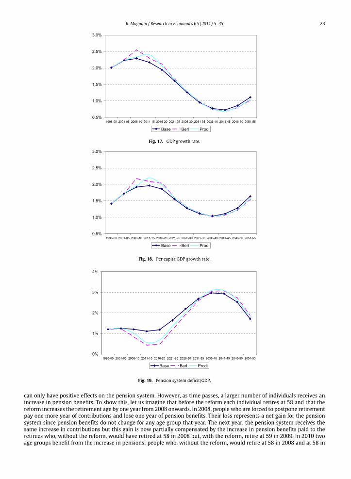
The evolution of GDP is mainly affected by the demographic projections. The strong reduction in the population agedbetween 20 and 64 implies negative rates of growth of the number of workers from 2015 to 2055 (Fig. 16) and explains thenegative evolution of the GDP growth (Fig. 17) and of the per capita GDP growth (Fig. 18). The evolution of the investmentratio plays another negative role in the economic growth, while the increase in the productivity growth rate and the increasein the employment rates are not sufficient to compensate the previous negative effects.
With respect to the base scenario, the reforms would induce an increase in the growth rate of the number of workersand consequently of the GDP growth rate and the per capita GDP growth rate until 2025. Afterwards, the economic growthrates are very similar in the three scenarios.
R. Magnani / Research in Economics 65 (2011) 5–35 21
Fig. 11. Wage, per unit of effective labour.
Fig. 12. Interest rate.
Fig. 13. Time devoted to schooling.
5.2. Effects of the Berlusconi and Prodi reforms on the pension system
Figs. 19 and 20 show the evolution of the pension system in terms of expenditures and deficits produced. We see thatinitially the two reforms that increase the retirement age have a significant positive impact on the financial situation of thepension system with respect to the base scenario, both in terms of the deficit and of the aggregate expenditure, as a ratio toGDP. For example, the Berlusconi reform makes it possible to reduce the ratio of the deficit to GDP of about 0.7% points in2015 and 0.3 p.p. in 2030. As could be expected, the reduction in the pension deficits with the Prodi reform is less important
22 R. Magnani / Research in Economics 65 (2011) 5–35
Fig. 14. Productivity growth rate.
Fig. 15. Investments/GDP.
Fig. 16. Growth rate of the # of workers.
in the short run than with the Berlusconi reform. The reduction is 0.5 p.p. in 2015, 0.2 p.p. in 2030 with respect to the basescenario.
However, in the long run, the increase in the retirement age becomes completely ineffective. In year 2035, the two reformsdisplay the same ratio of the pension system deficit to GDP as in the base scenario, and afterwards, this ratio becomes moreimportant than in the base case.
In order to understand the reason behind the inefficiency of these reforms in the long run, we have to consider thatan increase in the retirement age induces, for individuals obliged to postpone retirement, a present loss (represented bythe additional contributions paid and by the foregone pension benefits) and future gains (represented by the increase inthe value of the pension thereafter). In the early years of the introduction of the reform, the increase in the retirement age
R. Magnani / Research in Economics 65 (2011) 5–35 23
Fig. 17. GDP growth rate.
Fig. 18. Per capita GDP growth rate.
Fig. 19. Pension system deficit/GDP.
can only have positive effects on the pension system. However, as time passes, a larger number of individuals receives anincrease in pension benefits. To show this, let us imagine that before the reform each individual retires at 58 and that thereform increases the retirement age by one year from 2008 onwards. In 2008, people who are forced to postpone retirementpay one more year of contributions and lose one year of pension benefits. Their loss represents a net gain for the pensionsystem since pension benefits do not change for any age group that year. The next year, the pension system receives thesame increase in contributions but this gain is now partially compensated by the increase in pension benefits paid to theretirees who, without the reform, would have retired at 58 in 2008 but, with the reform, retire at 59 in 2009. In 2010 twoage groups benefit from the increase in pensions: people who, without the reform, would retire at 58 in 2008 and at 58 in
24 R. Magnani / Research in Economics 65 (2011) 5–35
Fig. 20. Pension expenditure/GDP.
Table 4aRate of return on contributions; native employees; base scenario.Source: Author’s calculations.
Retirement age 57 58 59 60 61 62 63 64 65Years of contributions 35 36 37 38 39 40 41 42 43
2001–05 3.20% 3.05% 2.89% 2.73% 2.45% 2.30% 2.14% 1.98% 1.81%2006–10 3.29% 3.14% 2.98% 2.82% 2.51% 2.36% 2.20% 2.04% 1.86%2011–15 3.33% 3.18% 3.01% 2.84% 2.52% 2.36% 2.19% 2.01% 1.83%2016–20 2.90% 2.78% 2.66% 2.53% 2.34% 2.24% 2.13% 2.03% 1.92%2021–25 2.77% 2.66% 2.56% 2.45% 2.29% 2.21% 2.12% 2.03% 1.93%2026–30 2.57% 2.49% 2.40% 2.31% 2.20% 2.13% 2.06% 1.98% 1.90%2031–35 2.21% 2.16% 2.10% 2.05% 2.01% 1.97% 1.92% 1.87% 1.82%2036–40 2.06% 2.01% 1.97% 1.91% 1.88% 1.85% 1.80% 1.76% 1.71%2041–45 1.91% 1.88% 1.83% 1.79% 1.76% 1.73% 1.69% 1.64% 1.60%2046–50 1.80% 1.77% 1.73% 1.69% 1.66% 1.63% 1.59% 1.55% 1.51%2051–55 1.75% 1.72% 1.68% 1.64% 1.62% 1.59% 1.55% 1.51% 1.47%
2009 but, with the reform, are constrained to work one additional year. And so on. So, as time passes by, the number ofindividuals who earn a greater level of pension benefits increases and the increase in the pension expenditure compensatesthe increase in the social contributions paid by the workers obliged to work more, and the reform ceases to be effective.
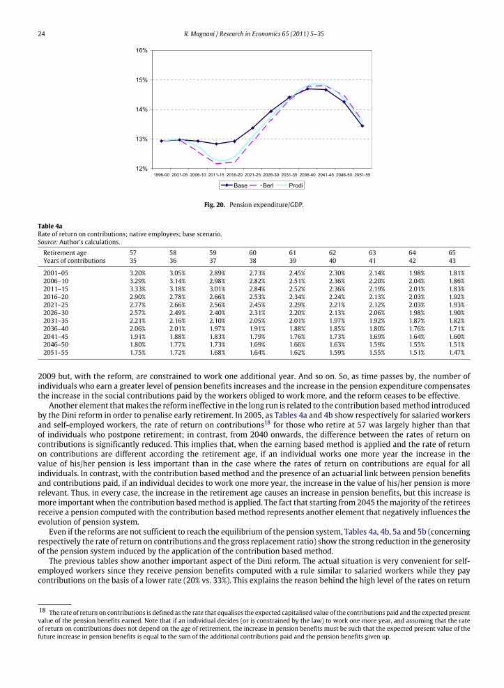
Another element thatmakes the reform ineffective in the long run is related to the contribution basedmethod introducedby the Dini reform in order to penalise early retirement. In 2005, as Tables 4a and 4b show respectively for salaried workersand self-employed workers, the rate of return on contributions18 for those who retire at 57 was largely higher than thatof individuals who postpone retirement; in contrast, from 2040 onwards, the difference between the rates of return oncontributions is significantly reduced. This implies that, when the earning based method is applied and the rate of returnon contributions are different according the retirement age, if an individual works one more year the increase in thevalue of his/her pension is less important than in the case where the rates of return on contributions are equal for allindividuals. In contrast, with the contribution based method and the presence of an actuarial link between pension benefitsand contributions paid, if an individual decides to work one more year, the increase in the value of his/her pension is morerelevant. Thus, in every case, the increase in the retirement age causes an increase in pension benefits, but this increase ismore important when the contribution basedmethod is applied. The fact that starting from 2045 themajority of the retireesreceive a pension computed with the contribution basedmethod represents another element that negatively influences theevolution of pension system.
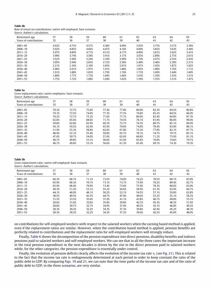
Even if the reforms are not sufficient to reach the equilibrium of the pension system, Tables 4a, 4b, 5a and 5b (concerningrespectively the rate of return on contributions and the gross replacement ratio) show the strong reduction in the generosityof the pension system induced by the application of the contribution based method.
The previous tables show another important aspect of the Dini reform. The actual situation is very convenient for self-employed workers since they receive pension benefits computed with a rule similar to salaried workers while they paycontributions on the basis of a lower rate (20% vs. 33%). This explains the reason behind the high level of the rates on return
18 The rate of return on contributions is defined as the rate that equalises the expected capitalised value of the contributions paid and the expected presentvalue of the pension benefits earned. Note that if an individual decides (or is constrained by the law) to work one more year, and assuming that the rateof return on contributions does not depend on the age of retirement, the increase in pension benefits must be such that the expected present value of thefuture increase in pension benefits is equal to the sum of the additional contributions paid and the pension benefits given up.
R. Magnani / Research in Economics 65 (2011) 5–35 25
Table 4bRate of return on contributions; native self-employed; base scenario.Source: Author’s calculations.
Retirement age 57 58 59 60 61 62 63 64 65Years of contributions 35 36 37 38 39 40 41 42 43
2001–05 4.92% 4.75% 4.57% 4.38% 4.09% 3.93% 3.75% 3.57% 3.38%2006–10 5.02% 4.85% 4.66% 4.47% 4.16% 4.00% 3.82% 3.63% 3.44%2011–15 5.07% 4.89% 4.71% 4.51% 4.17% 4.00% 3.81% 3.62% 3.41%2016–20 3.90% 3.74% 3.58% 3.41% 3.17% 3.03% 2.89% 2.75% 2.61%2021–25 3.52% 3.38% 3.24% 3.10% 2.90% 2.79% 2.67% 2.55% 2.43%2026–30 3.05% 2.94% 2.83% 2.72% 2.58% 2.49% 2.40% 2.30% 2.21%2031–35 2.21% 2.16% 2.10% 2.05% 2.01% 1.97% 1.92% 1.87% 1.82%2036–40 2.06% 2.01% 1.97% 1.91% 1.88% 1.85% 1.80% 1.76% 1.71%2041–45 1.91% 1.88% 1.83% 1.79% 1.76% 1.73% 1.69% 1.64% 1.60%2046–50 1.80% 1.77% 1.73% 1.69% 1.66% 1.63% 1.59% 1.55% 1.51%2051–55 1.75% 1.72% 1.68% 1.64% 1.62% 1.59% 1.55% 1.51% 1.47%
Table 5aGross replacement ratio; native employees; base scenario.Source: Author’s calculations.
Retirement age 57 58 59 60 61 62 63 64 65Years of contributions 35 36 37 38 39 40 41 42 43
2001–05 70.3% 72.7% 75.0% 77.4% 77.8% 80.0% 82.3% 84.5% 86.8%2006–10 70.1% 72.5% 74.9% 77.3% 77.5% 79.8% 82.2% 84.5% 86.9%2011–15 70.2% 72.7% 75.2% 77.6% 77.7% 80.0% 82.4% 84.8% 87.3%2016–20 62.8% 65.6% 68.6% 71.7% 74.5% 78.1% 81.9% 86.0% 90.4%2021–25 59.8% 62.8% 65.9% 69.3% 72.7% 76.5% 80.7% 85.1% 89.9%2026–30 56.1% 59.2% 62.4% 65.9% 70.0% 74.0% 78.4% 83.0% 88.1%2031–35 51.9% 55.3% 58.8% 62.6% 67.8% 72.3% 77.0% 82.1% 87.7%2036–40 48.9% 52.1% 55.4% 59.0% 65.7% 70.1% 74.7% 79.7% 85.1%2041–45 47.6% 50.7% 54.0% 57.6% 62.6% 66.8% 71.2% 75.9% 81.1%2046–50 46.7% 49.8% 53.1% 56.6% 61.6% 65.6% 70.0% 74.6% 79.7%2051–55 46.7% 49.8% 53.1% 56.6% 61.3% 65.4% 69.7% 74.3% 79.3%
Table 5bGross replacement ratio; native self-employed; base scenario.Source: Author’s calculations.
Retirement age 57 58 59 60 61 62 63 64 65Years of contributions 35 36 37 38 39 40 41 42 43
2001–05 66.3% 68.7% 71.1% 73.5% 74.0% 76.2% 78.5% 80.7% 83.0%2006–10 65.9% 68.3% 70.7% 73.1% 73.7% 75.9% 78.2% 80.4% 82.7%2011–15 65.9% 68.4% 70.9% 73.4% 73.6% 75.9% 78.3% 80.6% 83.0%2016–20 49.3% 51.2% 53.1% 55.2% 56.6% 58.9% 61.3% 63.9% 66.7%2021–25 44.1% 46.0% 48.1% 50.2% 52.1% 54.5% 57.1% 59.8% 62.8%2026–30 38.5% 40.5% 42.5% 44.7% 47.0% 49.6% 52.2% 55.1% 58.2%2031–35 31.5% 33.5% 35.6% 37.9% 41.1% 43.8% 46.7% 49.8% 53.1%2036–40 29.6% 31.6% 33.6% 35.8% 39.8% 42.5% 45.3% 48.3% 51.6%2041–45 28.8% 30.7% 32.7% 34.9% 37.9% 40.5% 43.1% 46.0% 49.2%2046–50 28.3% 30.2% 32.2% 34.3% 37.3% 39.8% 42.4% 45.2% 48.3%2051–55 28.3% 30.2% 32.2% 34.3% 37.2% 39.6% 42.2% 45.0% 48.0%
on contributions for self-employedworkers with respect to the salaried workers when the earning basedmethod is applied,even if the replacement ratios are similar. However, when the contribution based method is applied, pension benefits areperfectly related to contributions and the replacement ratio for self-employed workers will strongly reduce.
Finally, Table 6 shows the decomposition of the pension expenditure into direct pensions, disability benefits and indirectpensions paid to salaried workers and self-employed workers. We can see that in all the three cases the important increasein the total pension expenditure in the next decades is driven by the rise in the direct pensions paid to salaried workerswhile, for the other categories, the pension expenditure is essentially under control.
Finally, the evolution of pension deficits clearly affects the evolution of the income tax rate τt (see Fig. 21). This is relatedto the fact that the income tax rate is endogenously determined at each period in order to keep constant the ratio of thepublic debt to GDP. By comparing Figs. 19 and 21, we can note that the time paths of the income tax rate and of the ratio ofpublic debt to GDP, in the three scenarios, are very similar.

26 R. Magnani / Research in Economics 65 (2011) 5–35
Fig. 21. Income tax rate, normalized to 1 in 2001–2005.
Table 6Pension expenditure/GDP.Source: Author’s calculations.
2001–05 2006–10 2011–15 2021–25 2031–35 2041–45 2051–55
Base 8.09% 8.05% 8.03% 8.53% 9.19% 9.29% 8.50%Direct pensions Berl 8.09% 7.76% 7.45% 8.11% 9.00% 9.23% 8.48%
Prodi 8.09% 7.91% 7.60% 8.33% 9.14% 9.35% 8.49%Base 0.61% 0.61% 0.60% 0.62% 0.69% 0.72% 0.66%
Employees Disability benefits Berl 0.61% 0.61% 0.60% 0.63% 0.71% 0.76% 0.70%Prodi 0.61% 0.61% 0.60% 0.62% 0.69% 0.74% 0.69%Base 1.82% 1.81% 1.81% 1.87% 2.08% 2.19% 2.03%
Indirect pensions Berl 1.82% 1.80% 1.79% 1.87% 2.13% 2.30% 2.15%Prodi 1.82% 1.81% 1.79% 1.85% 2.08% 2.24% 2.10%
Base 1.89% 1.89% 1.83% 1.80% 1.84% 1.82% 1.64%Direct pensions Berl 1.89% 1.85% 1.77% 1.77% 1.85% 1.84% 1.66%
Prodi 1.89% 1.85% 1.76% 1.76% 1.84% 1.83% 1.65%Base 0.26% 0.27% 0.26% 0.26% 0.29% 0.32% 0.30%
Self-employed Disability benefits Berl 0.26% 0.27% 0.26% 0.26% 0.30% 0.33% 0.32%Prodi 0.26% 0.27% 0.26% 0.26% 0.29% 0.32% 0.31%Base 0.30% 0.30% 0.29% 0.29% 0.31% 0.33% 0.30%
Indirect pensions Berl 0.30% 0.30% 0.29% 0.29% 0.32% 0.34% 0.32%Prodi 0.30% 0.30% 0.29% 0.29% 0.32% 0.33% 0.31%
5.3. Generational accounting
We now use the generational accounting approach introduced by Auerbach et al. (1994) to evaluate the gains and thelosses for each generation associated with the introduction of the Berlusconi and the Prodi reforms. For each generation, wecompute the ratio of the expected present value of the revenues (pension benefits and per capita government expenditures)to the expected present value of the payments (income taxes and social security contributions).
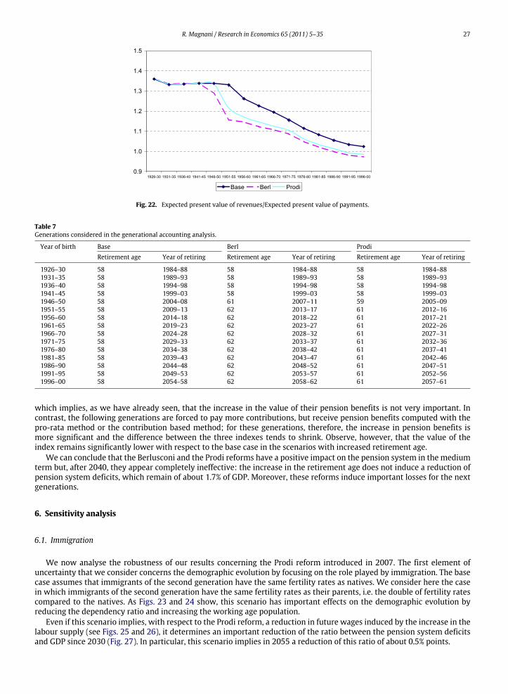
As shown in Table 7, the first generation considered in the generational accounting analysis is that born in the period1926–1930, while the last one is that born in the period 1996–2000. The analysis concerns only native salaried workers whostart working at 22.
In the base scenario, all the generations stop working at 58. In the simulation concerning the Berlusconi reform, allthe generations born before 1946 stop working at 58, the generation born in the period 1946–1950 stops working at 61,and all the generations born after 1950 stop working at 62. In the simulation concerning the Berlusconi reform, all thegenerations born before 1946 stop working at 58, the generation born in the period 1946–1950 stops working at 59, and allthe generations born after 1950 stop working at 61.
The results of this analysis are shown in Fig. 22. First of all, by considering the base case, we note that the value of thisindex decreases starting from the generation born in the period 1956–1960. The reason for this decrease is the reduction ofthe generosity of the pension system related to the introduction of the pro-rata method and the contribution basedmethod,and the strong increase in the income tax rate necessary to keep constant the ratio between the public debt and the GDP(see Fig. 21).
With respect to the base case, the Berlusconi reform causes a sharp fall of the index for the generation born in 1946–1950,which is the first generation who must work until 61, while with the Prodi reform the reduction of the index begins for thegeneration born in 1951–1955. It is important to note that the generations born in the periods 1946–1950 and1951–1955 arethe first generations forced to pay more contributions and they receive a pension computed with the earning basedmethod
R. Magnani / Research in Economics 65 (2011) 5–35 27
Fig. 22. Expected present value of revenues/Expected present value of payments.
Table 7Generations considered in the generational accounting analysis.
Year of birth Base Berl ProdiRetirement age Year of retiring Retirement age Year of retiring Retirement age Year of retiring
1926–30 58 1984–88 58 1984–88 58 1984–881931–35 58 1989–93 58 1989–93 58 1989–931936–40 58 1994–98 58 1994–98 58 1994–981941–45 58 1999–03 58 1999–03 58 1999–031946–50 58 2004–08 61 2007–11 59 2005–091951–55 58 2009–13 62 2013–17 61 2012–161956–60 58 2014–18 62 2018–22 61 2017–211961–65 58 2019–23 62 2023–27 61 2022–261966–70 58 2024–28 62 2028–32 61 2027–311971–75 58 2029–33 62 2033–37 61 2032–361976–80 58 2034–38 62 2038–42 61 2037–411981–85 58 2039–43 62 2043–47 61 2042–461986–90 58 2044–48 62 2048–52 61 2047–511991–95 58 2049–53 62 2053–57 61 2052–561996–00 58 2054–58 62 2058–62 61 2057–61
which implies, as we have already seen, that the increase in the value of their pension benefits is not very important. Incontrast, the following generations are forced to pay more contributions, but receive pension benefits computed with thepro-rata method or the contribution based method; for these generations, therefore, the increase in pension benefits ismore significant and the difference between the three indexes tends to shrink. Observe, however, that the value of theindex remains significantly lower with respect to the base case in the scenarios with increased retirement age.
We can conclude that the Berlusconi and the Prodi reforms have a positive impact on the pension system in the mediumterm but, after 2040, they appear completely ineffective: the increase in the retirement age does not induce a reduction ofpension system deficits, which remain of about 1.7% of GDP. Moreover, these reforms induce important losses for the nextgenerations.
6. Sensitivity analysis
6.1. Immigration
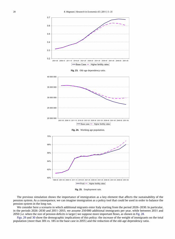
We now analyse the robustness of our results concerning the Prodi reform introduced in 2007. The first element ofuncertainty that we consider concerns the demographic evolution by focusing on the role played by immigration. The basecase assumes that immigrants of the second generation have the same fertility rates as natives. We consider here the casein which immigrants of the second generation have the same fertility rates as their parents, i.e. the double of fertility ratescompared to the natives. As Figs. 23 and 24 show, this scenario has important effects on the demographic evolution byreducing the dependency ratio and increasing the working age population.
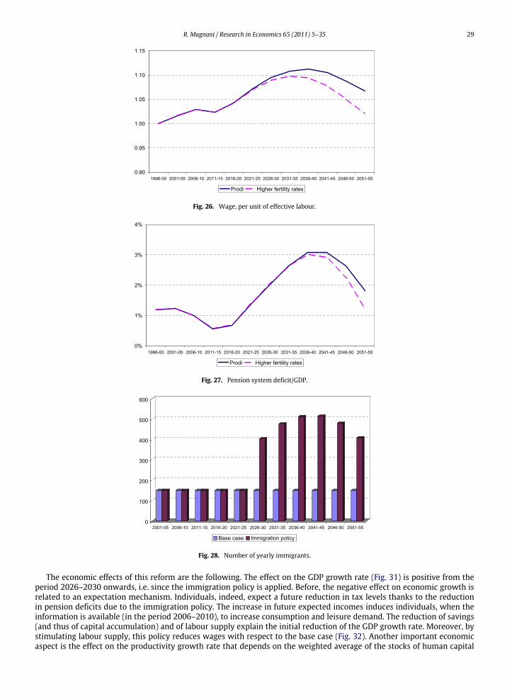
Even if this scenario implies, with respect to the Prodi reform, a reduction in future wages induced by the increase in thelabour supply (see Figs. 25 and 26), it determines an important reduction of the ratio between the pension system deficitsand GDP since 2030 (Fig. 27). In particular, this scenario implies in 2055 a reduction of this ratio of about 0.5% points.
28 R. Magnani / Research in Economics 65 (2011) 5–35
Fig. 23. Old-age dependency ratio.
Fig. 24. Working age population.
Fig. 25. Employment rate.
The previous simulation shows the importance of immigration as a key element that affects the sustainability of thepension system. As a consequence, we can imagine immigration as a policy tool that could be used in order to balance thepension system in the long run.
We consider here a scenario in which additional migrants enter Italy starting from the period 2026–2030. In particular,in the periods 2026–2030 and 2051–2055, we assume 250000 additional immigrants per year, while between 2031 and2050 (i.e. when the size of pension deficits is larger) we suppose more important flows, as shown in Fig. 28.
Figs. 29 and 30 show the demographic implications of this policy: the increase of the weight of immigrants on the totalpopulation (more than 30% vs. 18% in the base case in 2055) and the reduction of the old-age dependency ratio.
R. Magnani / Research in Economics 65 (2011) 5–35 29
Fig. 26. Wage, per unit of effective labour.
Fig. 27. Pension system deficit/GDP.
Fig. 28. Number of yearly immigrants.
The economic effects of this reform are the following. The effect on the GDP growth rate (Fig. 31) is positive from theperiod 2026–2030 onwards, i.e. since the immigration policy is applied. Before, the negative effect on economic growth isrelated to an expectation mechanism. Individuals, indeed, expect a future reduction in tax levels thanks to the reductionin pension deficits due to the immigration policy. The increase in future expected incomes induces individuals, when theinformation is available (in the period 2006–2010), to increase consumption and leisure demand. The reduction of savings(and thus of capital accumulation) and of labour supply explain the initial reduction of the GDP growth rate. Moreover, bystimulating labour supply, this policy reduces wages with respect to the base case (Fig. 32). Another important economicaspect is the effect on the productivity growth rate that depends on the weighted average of the stocks of human capital
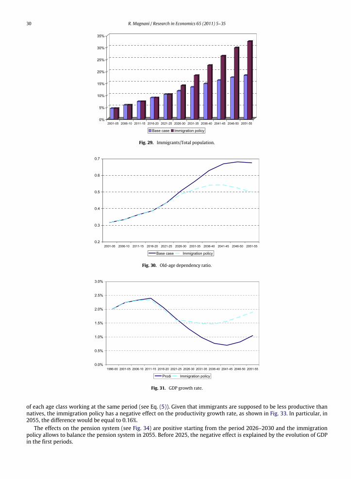
30 R. Magnani / Research in Economics 65 (2011) 5–35
Fig. 29. Immigrants/Total population.
Fig. 30. Old-age dependency ratio.
Fig. 31. GDP growth rate.
of each age class working at the same period (see Eq. (5)). Given that immigrants are supposed to be less productive thannatives, the immigration policy has a negative effect on the productivity growth rate, as shown in Fig. 33. In particular, in2055, the difference would be equal to 0.16%.
The effects on the pension system (see Fig. 34) are positive starting from the period 2026–2030 and the immigrationpolicy allows to balance the pension system in 2055. Before 2025, the negative effect is explained by the evolution of GDPin the first periods.

R. Magnani / Research in Economics 65 (2011) 5–35 31
Fig. 32. Wage, per unit of effective labour.
Fig. 33. Productivity growth rate.
Fig. 34. Pension system deficit/GDP.
6.2. Pension benefits
Another important element of uncertainty in our simulation exercise concerns the value of pension benefits. Theuncertainty is related to the fact that the Dini reform (Law 335/1995) states that the transformation coefficients used inthe computation of pension benefits, with the contribution based method and the pro-rata method, must be updated everyten years according to economic and demographic evolutions, in particular the increase in life expectancy. In 2005, i.e. tenyears after the introduction of the Dini reform, no revision of the transformation coefficients were made, reflecting theenormous difficulty, in the Italian political context, to reform the pension system in a way that penalises the retirees.
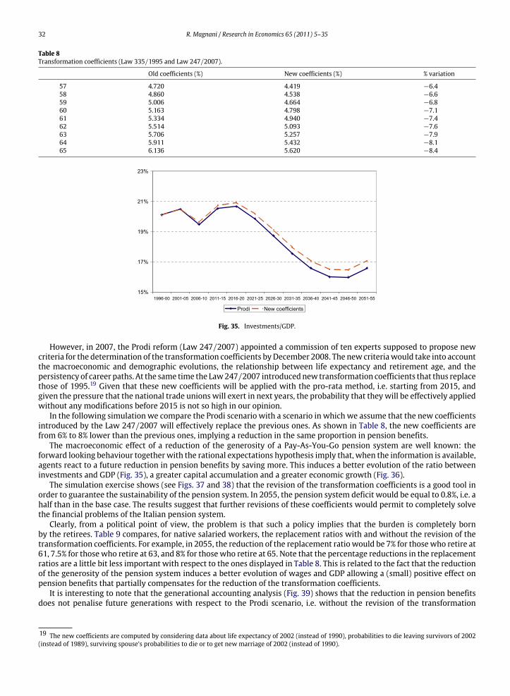
32 R. Magnani / Research in Economics 65 (2011) 5–35
Table 8Transformation coefficients (Law 335/1995 and Law 247/2007).
Old coefficients (%) New coefficients (%) % variation
57 4.720 4.419 −6.458 4.860 4.538 −6.659 5.006 4.664 −6.860 5.163 4.798 −7.161 5.334 4.940 −7.462 5.514 5.093 −7.663 5.706 5.257 −7.964 5.911 5.432 −8.165 6.136 5.620 −8.4
Fig. 35. Investments/GDP.
However, in 2007, the Prodi reform (Law 247/2007) appointed a commission of ten experts supposed to propose newcriteria for the determination of the transformation coefficients byDecember 2008. The new criteriawould take into accountthe macroeconomic and demographic evolutions, the relationship between life expectancy and retirement age, and thepersistency of career paths. At the same time the Law247/2007 introducednew transformation coefficients that thus replacethose of 1995.19 Given that these new coefficients will be applied with the pro-rata method, i.e. starting from 2015, andgiven the pressure that the national trade unions will exert in next years, the probability that they will be effectively appliedwithout any modifications before 2015 is not so high in our opinion.
In the following simulation we compare the Prodi scenario with a scenario in which we assume that the new coefficientsintroduced by the Law 247/2007 will effectively replace the previous ones. As shown in Table 8, the new coefficients arefrom 6% to 8% lower than the previous ones, implying a reduction in the same proportion in pension benefits.
The macroeconomic effect of a reduction of the generosity of a Pay-As-You-Go pension system are well known: theforward looking behaviour togetherwith the rational expectations hypothesis imply that, when the information is available,agents react to a future reduction in pension benefits by saving more. This induces a better evolution of the ratio betweeninvestments and GDP (Fig. 35), a greater capital accumulation and a greater economic growth (Fig. 36).
The simulation exercise shows (see Figs. 37 and 38) that the revision of the transformation coefficients is a good tool inorder to guarantee the sustainability of the pension system. In 2055, the pension system deficit would be equal to 0.8%, i.e. ahalf than in the base case. The results suggest that further revisions of these coefficients would permit to completely solvethe financial problems of the Italian pension system.
Clearly, from a political point of view, the problem is that such a policy implies that the burden is completely bornby the retirees. Table 9 compares, for native salaried workers, the replacement ratios with and without the revision of thetransformation coefficients. For example, in 2055, the reduction of the replacement ratio would be 7% for thosewho retire at61, 7.5% for those who retire at 63, and 8% for those who retire at 65. Note that the percentage reductions in the replacementratios are a little bit less important with respect to the ones displayed in Table 8. This is related to the fact that the reductionof the generosity of the pension system induces a better evolution of wages and GDP allowing a (small) positive effect onpension benefits that partially compensates for the reduction of the transformation coefficients.
It is interesting to note that the generational accounting analysis (Fig. 39) shows that the reduction in pension benefitsdoes not penalise future generations with respect to the Prodi scenario, i.e. without the revision of the transformation
19 The new coefficients are computed by considering data about life expectancy of 2002 (instead of 1990), probabilities to die leaving survivors of 2002(instead of 1989), surviving spouse’s probabilities to die or to get new marriage of 2002 (instead of 1990).
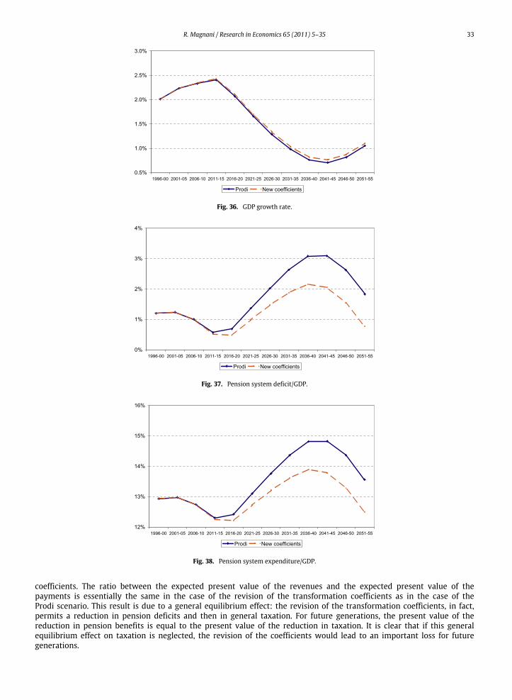
R. Magnani / Research in Economics 65 (2011) 5–35 33
Fig. 36. GDP growth rate.
Fig. 37. Pension system deficit/GDP.
Fig. 38. Pension system expenditure/GDP.
coefficients. The ratio between the expected present value of the revenues and the expected present value of thepayments is essentially the same in the case of the revision of the transformation coefficients as in the case of theProdi scenario. This result is due to a general equilibrium effect: the revision of the transformation coefficients, in fact,permits a reduction in pension deficits and then in general taxation. For future generations, the present value of thereduction in pension benefits is equal to the present value of the reduction in taxation. It is clear that if this generalequilibrium effect on taxation is neglected, the revision of the coefficients would lead to an important loss for futuregenerations.
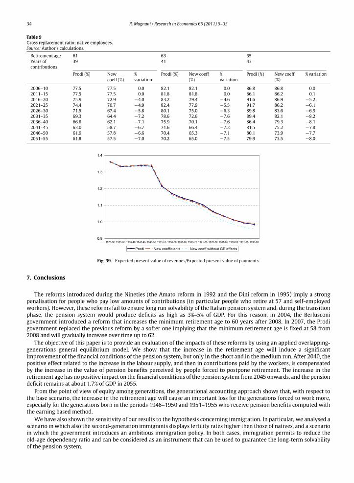
34 R. Magnani / Research in Economics 65 (2011) 5–35
Table 9Gross replacement ratio; native employees.Source: Author’s calculations.
Retirement age 61 63 65Years ofcontributions
39 41 43
Prodi (%) Newcoeff (%)
%variation
Prodi (%) New coeff(%)
%variation
Prodi (%) New coeff(%)
% variation
2006–10 77.5 77.5 0.0 82.1 82.1 0.0 86.8 86.8 0.02011–15 77.5 77.5 0.0 81.8 81.8 0.0 86.1 86.2 0.12016–20 75.9 72.9 −4.0 83.2 79.4 −4.6 91.6 86.9 −5.22021–25 74.4 70.7 −4.9 82.4 77.9 −5.5 91.7 86.2 −6.12026–30 71.5 67.4 −5.8 80.1 75.0 −6.3 89.8 83.6 −6.92031–35 69.3 64.4 −7.2 78.6 72.6 −7.6 89.4 82.1 −8.22036–40 66.8 62.1 −7.1 75.9 70.1 −7.6 86.4 79.3 −8.12041–45 63.0 58.7 −6.7 71.6 66.4 −7.2 81.5 75.2 −7.82046–50 61.9 57.8 −6.6 70.4 65.3 −7.1 80.1 73.9 −7.72051–55 61.8 57.5 −7.0 70.2 65.0 −7.5 79.9 73.5 −8.0
Fig. 39. Expected present value of revenues/Expected present value of payments.
7. Conclusions
The reforms introduced during the Nineties (the Amato reform in 1992 and the Dini reform in 1995) imply a strongpenalisation for people who pay low amounts of contributions (in particular people who retire at 57 and self-employedworkers). However, these reforms fail to ensure long run solvability of the Italian pension system and, during the transitionphase, the pension system would produce deficits as high as 3%–5% of GDP. For this reason, in 2004, the Berlusconigovernment introduced a reform that increases the minimum retirement age to 60 years after 2008. In 2007, the Prodigovernment replaced the previous reform by a softer one implying that the minimum retirement age is fixed at 58 from2008 and will gradually increase over time up to 62.
The objective of this paper is to provide an evaluation of the impacts of these reforms by using an applied overlapping-generations general equilibrium model. We show that the increase in the retirement age will induce a significantimprovement of the financial conditions of the pension system, but only in the short and in the medium run. After 2040, thepositive effect related to the increase in the labour supply, and then in contributions paid by the workers, is compensatedby the increase in the value of pension benefits perceived by people forced to postpone retirement. The increase in theretirement age has no positive impact on the financial conditions of the pension system from2045 onwards, and the pensiondeficit remains at about 1.7% of GDP in 2055.
From the point of view of equity among generations, the generational accounting approach shows that, with respect tothe base scenario, the increase in the retirement age will cause an important loss for the generations forced to work more,especially for the generations born in the periods 1946–1950 and 1951–1955 who receive pension benefits computed withthe earning based method.
We have also shown the sensitivity of our results to the hypothesis concerning immigration. In particular, we analysed ascenario in which also the second-generation immigrants displays fertility rates higher then those of natives, and a scenarioin which the government introduces an ambitious immigration policy. In both cases, immigration permits to reduce theold-age dependency ratio and can be considered as an instrument that can be used to guarantee the long-term solvabilityof the pension system.

R. Magnani / Research in Economics 65 (2011) 5–35 35
Finally, we analysed an important aspect of the Dini reform (1995). The transformation coefficients used in thecomputation of the pension benefits with the pro-rata method and the contribution based method are supposed to beupdated every ten years according to the evolution of several elements, especially the increase in life expectancy. In 2005,i.e. when the first revision would have been made and close to national elections, nothing happened. In 2007, the Prodigovernment proposed new transformation coefficients, but (i) at the same time, the Prodi reform appointed a commissionthat will propose before December 2008 new criteria for the determination of the transformation coefficients (ii) thetransformation coefficients will be applied starting from 2015, i.e. with the pro-rata method. This suggests that the newtransformation coefficients are likely to be modified before 2015. In any case, we have shown that the transformationcoefficients proposed with the Prodi reform would permit an important reduction in pension deficits. Moreover, even ifthis implies important income losses for the retirees, a generational accounting analysis shows that the future generationswill not be penalised, since the loss in pension benefits will be compensated by a lower taxation.
Acknowledgement
I would like to thank Jean Mercenier for very useful comments. All errors remain mine.
References
Aglietta, M., Chateau, J., Fayolle, J., Juillard, M., Le Cacheux, J., Le Garrec, G., Touze, V., 2007. Pension reforms in Europe: an investigation with a computableOLG world model. Economic Modelling 24, 481–505.
Auerbach, A., Kotlikoff, L., 1987. Dynamic Fiscal Policy. Cambridge University Press.Auerbach, A., Gokhale, J., Kotlikoff, L., 1994. Generational accounting: Ameaningful way to evaluate fiscal policy. Journal of Economic Perspectives 8, 73–94.Barro, R.J., 2001. Human capital and growth. In: Papers and Proceedings of the Hundred Thirteenth Annual Meeting of the American Economic Association.
American Economic Review 91 (2), 12–17.Börsh-Supan, A., Ludwing, A., Winter, A., 2006. Ageing, pension reform and capital flows. Economica 73, 625–658.Bouzahzaha, M., de la Croix, D., Docquier, F., 2002. Policy reforms and growth in computable OLG economies. Journal of Economic Dynamics and Control
26, 2093–2113.Chateau, J., Chojnicki, X., Magnani, R., 2009. Disparities in pension system and financial flows among European countries. Journal of Pension Economics and
Finance 8 (01), 1–33.Fougère, M, Mérette, M., 1999. Population ageing and economic growth in seven OECD countries. Economic Modelling 16, 411–427.Istat, 1998. Tavole di mortalità per provincia e regione di residenza.Istat, 2004. La presenza straniera in Italia: caratteristiche socio-demografiche. Permessi di soggiorno al 1 gennaio degli anni 2001, 2002, 2003.Istat, 2006. Previsioni demografiche nazionali. 1 gennaio 2005 - 1 gennaio 2050.Istat, 2007a. Statistiche della previdenza e dell’assistenza sociale. I trattamenti pensionistici. Anno 2005.Istat, 2007b. La popolazione straniera residente in Italia al 1 gennaio 2007.Lucas, R.J., 1988. On the mechanics of economic development. Journal of Monetary Economics 22, 3–42.Magnani, R., 2006. Vieillissement de la population en Italie et efficacité des réformesAmato et Dini: unmodèle d’é quilibre général à générations imbriquées.
Recherches Economiques de Louvain 72 (3), 287–338.Mayer, J., Riphahn, R., 1999. Fertility assimilation of immigrants: Evidence from count data models. IZA Discussion Paper. 1999, n. 52.Miles, D., 1999. Modelling the impact of demographic change upon the economy. The Economic Journal 109, 1–36.Nucleo di Valutazione della Spesa Previdenziale, 2006. Gli andamenti finanziari del sistema pensionistico obbligatorio.Ragioneria Generale dello Stato, 2006. Le tendenze di medio-lungo periodo del sistema pensionistico e socio-sanitario. Rapporto n. 8.Sadahiro, A., Shimasawa,M., 2003. The computable overlapping generationsmodel with an endogenous growthmechanism. EconomicModelling 20, 1–24.Storesletten, K., 2000. Sustaining fiscal policy through immigration. Journal of Political Economy 108, 300–323.Yaari, M.E., 1965. Uncertain lifetime, life insurance, and the theory of the consumer. Review of Economic Studies 32, 137–150.