A Generalized Nonlinear IV Unit Root Test for Panel Data With

Cross Sectional Dependence

Shaoping Wang, Jisheng Yang, and Zinai Li1

Abstract: This paper proposes an unit root test for panel data with cross sectional dependence.

The proposed test generalizes the nonlinear IV unit root test proposed by Chang (2002). The main

idea is to eliminate the cross sectional dependence through covariance matrix weighting and then

apply Chang’s test to the weighted data. Under some sufficient conditions, we show that the

proposed test statistic has limiting standard normal distribution under the null hypothesis and

converges to negative infinity under the alternative hypothesis. The finite sample performance of

the proposed test is evaluated through a small-scale simulation study. The simulation results show

that proposed test compares favorably to other alternative tests when cross sectional dependence

exists.

JEL classification: C12; C15; C33.

Keywords: Panel unit root test, Nonlinear instrument, t-ratio, Cross sectional dependence.

1. Introduction

Testing for the presence of unit root in panel data has received considerable attention

from time series econometricians. Many testing procedures have been proposed and

their statistical properties have been established. Hurlin and Mignon (2004) provide a

good summary of the literature up to that date. Generally, the proposed tests can be

grouped, based on their assumptions on the cross sectional dependence, into two 1 Shaoping Wang, School of Economics, Huazhong University of Science and Technology, China. Jisheng Yang, School of Economics, Huazhong Universiy of Science and Technology, China. Zinai Li, School of Economics and Management, Tsinghua University, China. Wang’s research are supported by Chinese National Social Science Foundation Grant 05BJY012 and Chinese National Science Foundation Grant 70571026.

1

groups. The first group of tests assume cross sectional independence. This group

includes Levin and Lin (1992,1993) and Levin, Lin and Chu (2002) who propose unit

root tests for homogeneous panels, and Harris and Tzavalis (1999), Im, Pesaran and

Shin (1997, 2003), Maddala and Wu (1999), and Choi (1999,2001) who propose tests

for heterogeneous panels. The test proposed by Im, Pesaran and Shin (1997,2003) is a

simple application of the usual ADF tests to each individual, while the tests proposed

by Maddala and Wu (1999), and Choi (1999,2001) use the p-values from the usual

ADF tests applied to each individual.

The second group of tests does not assume cross sectional independence. This

group include Flôres, Preumont and Szafarz (1995), Tayor and Sarno (1998), Breitung

and Das (2004), Bai and Ng (2001, 2004)，Moon and Perron (2004)，Phillips and Sul

(2003)，and Pesaran (2003), Choi (2002), and Chang (2002). The first three studies do

not explicitly model the form of the cross sectional dependence. For instance, the test

proposed by Flôres, Preumont and Szafarz (1995) is based on a seemingly unrelated

regression (SUR) system where each individual is treated as one equation. Their test

statistic has a nonstandard asymptotic distribution. Tayor and Sarno (1998) propose a

Wald test. The asymptotic distribution of their test is unknown. Breitung and Das

(2004) present simple ADF test applied to pooled samples with robust standard error.

The next five studies explicitly model the form of the cross sectional dependence

through common factors. For example, Bai and Ng (2001,2004)，Moon and Perron

(2004)，Phillips and Sul (2003)，and Pesaran (2003) assume that the dependence of the

cross sectional units is due to some common factors for all individuals. They suggest

first applying the principal component method to eliminate the common factors

(hence the correlation of cross-sectional units), then applying the ADF type test. Choi

(2002) models the cross sectional dependence by time-invariant common factors. He

suggests using demean and/or de-trend method developed by Elliott, Rothenberg and

Stock (1996) to eliminate the common factors. His test statistic has limiting standard

normal distribution. Chang (2002), on the other hand, don’t assumes a particular form

of the cross sectional dependence. Instead of the usual t-ratio on the lagged dependent

2

variable obtained from applying least squares regression to each individual, Chang

(2002) suggests using the t-ratio on the lagged dependent variable obtained from

applying nonlinear instrumental variable estimation to each individual. The nonlinear

instrument allows her to obtain a remarkable result that the t-ratios of the coefficients

on the lagged dependent variable are asymptotically independent across individuals

regardless of the cross sectional dependence. She shows that her test statistic has a

limiting standard normal distribution.

Given Chang’s (2002) remarkable theoretical result, it is interesting to see how her

test performs in finite samples. Although Change demonstrates that her test performs

well in her design, it is worthwhile to have a more extensive simulation study on

broader designs. Im and Pesaran (2003) provide such a simulation study. They find

that Chang test performs well in finite samples only when the cross sectional

dependence is low. When the cross sectional dependence is moderate to high, Chang

test does not perform well. The reason for the poor performance is that the cross

sectional dependence is not fully eliminated by the instrument when the cross

sectional dependence is moderate to high, and consequently the t-ratios are not

approximately statistically independent. As a result, the finite sample distribution of

Chang test statistic is not even close to normal.

In light of the findings of Im and Pesaran (2003), one obvious remedy is to remove

the cross sectional dependence before applying Chang test. This is exactly the

approach taken in this paper. We suggest first weighting data by the contemporary

covariance matrix and then applying Chang test to the weighted data. We show that

our test, like Chang test, has a limiting standard normal distribution under the null

hypothesis of unit root. The question then is whether our test has better finite sample

performance when cross sectional dependence is moderate to high. Our simulation

study show that our test performs much better than Chang test when the cross

sectional dependence is moderate to high. Moreover, even when the cross sectional

dependence is low, our test performs at least as good as Chang test.

3

The remainder of this paper is organized as follows. Section 2 sets up the model.

Section 3 presents the test statistic and its asymptotic distribution. Section 4 reports on

a simulation study. Section 5 concludes.

2. Model and Preliminaries

Let index individual and let t index time. Suppose that is generated

according to the following process：

i ity

, 1it i i t ity y uα −= + ， 1, ,i N= ， Tt ,1= , (1)

where iα denotes the coefficient on the lagged dependent variable and denotes

the error term which follows the following AR(p) process:

itu

ititi uLW ε=)( ， ∑ =

−=p

kk

kii zzW

1 ,1)( ρ (2)

where L is the lag operator, },...,2,1;,...,2,1,{ , Nipkki ==ρ denote the

autoregressive coefficients, and denotes some integer that is known and fixed. We

are interested in testing the null hypothesis of unit root for all individuals:

p

:0H 1=iα , for all 1, ,i N=

against the alternative hypothesis of stationary:

:1H 1<iα for some . i

Denote . The following conditions are familiar in time series

literature and are similar to those imposed by Chang (2002).

)',...,( 1 NttNt εεε =

Assumption 1： for all 0)( ≠zW i 1z ≤ and 1, ,i N= .

Assumption 2：(i) are independent and identically distributed

and its distribution is absolutely continuous with respect to Lebesgue measure; (ii)

TtNt ,...,2,1, =ε

4

Ntε

has mean zero and covariance matrix )( ijσ=Σ ; (iii) satisfies

for some and has a characteristic function

Ntε

∞<}|{| lNtE ε 4l > ϕ that

satisfies 0)(lim =∞→

λϕλ τ

λ for some 0>τ .

Assumption 1 ensures that the AR(p) process in (2) is invertible. Assumption 2

restricts the distribution of error term.

Denote

, ， , , ⎟⎟⎟⎞

⎜⎜⎜⎛

=+pi

i

yy

1,

⎠⎝ Tiy , ⎠⎝ −1,Tiy ⎠⎝ Tix ,' ⎠⎝ Ti,ε⎟⎟⎟⎞

⎜⎜⎜⎛

=−

,

1,

pi

i

yy

⎟⎟⎟⎞

⎜⎜⎜⎛

=+pi

i

xX

1,'

⎟⎟⎟⎞

⎜⎜⎜⎛

=+pi

i

1,εε

where . Model (1) – (2) can be rewritten as: ),,( ,1,'

ptitiit yyx −− ΔΔ=

iiiiii Xyy εβα ++= −1, , (3)

where iβ denote the coefficients to be estimated. Equation (3) is often estimated by

simple OLS. Under the unit root hypothesis, it is well known that the asymptotic

distribution of the t-ratio for the OLS estimator iα obtained from (3) is asymmetric,

and not the usual t-distribution. Instead of applying OLS regression, Chang (2002)

suggests an instrumental variable estimation with , 1( i tF y )− as instrument for , 1i ty − ,

where F is any function satisfying:

Assumption 3： is regularly integrable and satisfy . )(xF ∫∞

∞−≠ 0)(xxF

Under Assumptions 1 – 3, Chang (2002) derives the following key result:

∑=

−− ⎯→⎯T

tjttjitti yFyFT

11,1, 0])(][)([ εε (4)

5

as . This result states that the t-ratios of ∞→T iα and jα are asymptotically

uncorrelated regardless of the cross sectional dependence and hence the test statistic,

∑ ==

N

iN it

NS

1

1α , where is the t-ratio for the instrumental variable estimator of

itα

iα , has a limiting standard normal distribution. Chang (2002) considers a special

instrument , 1, 1 , 1( ) i i tc y

i t i tF y y e −−− −= with as a constant, which obviously satisfies

Assumption 3. In her simulation design, however, Chang sets to:

ic

ic

12/1 −−= sKTc ii (5)

with . Such selected is inversely proportional to ∑=− Δ= iT

t iti yTs1

212 )( ic1

2iT as

well as the sample standard error of it ity uΔ = . In their simulation study, Im and

Pesaran (2003) find that, when is a fixed constant, the distribution of the t-ratio of

the IV estimator

ic

iα is skewed to the right when cross sectional dependence exists，

particularly when T is relatively small. In this case, Chang test is grossly under-sized.

When is chosen as in (5), their simulation reveals that the distribution of the

t-ratio of

ic

iα centers around zero，and Chang test in this case performs better. Im and

Pesaran (2003) also find that, when the constant in (5) is used, the t-ratios of iα and

jα will not be asymptotically uncorrelated if the underlying series are cross-sectional

correlated. Consequently, the test statistic SN does not have limiting standard normal

distribution when the cross sectional dependence exists.

Im and Pesaran (2003) re-examine the finite sample properties of Chang test and

find that the finite sample properties critically depend on the choice of the cross

sectional covariance matrix of the error terms. Chang test performs reasonably well

when cross sectional dependence is low but poorly when the cross sectional

dependence is moderate to high.

6

3. Generalized Chang test

In light of these findings, we propose a two-step procedure. In the first step, the

cross sectional dependence is eliminated through the contemporary covariance matrix

weighting. In the second step, Chang test is applied to the weighted data. Let Γ

denote the symmetric and invertible matrix satisfying Σ=ΓΓ ' , in which is the

cross sectional covariance matrix. Denote ，with as the

identity matrix. Denote

Σ

)( 11

−−− ⊗Γ=Λ pTI 1−− pTI

)1()1( −−×−− pTpT

， ),,()),,(( **11

*NN yyvecyyvecY =Λ=

， ),,()),,(( *1,

*1,11,1,1

*1 −−−−− =Λ= NN yyvecyyvecY

, );,()),,(( *,

*,1,,1

*kNkkNkk yyvecyyvecY −−−−− ΔΔ=ΔΛ=Δ pj ,,1= , (6)

. ),,()),,(( **11

*NN vecvec εεεεε =Λ=

),,( *,

*1,

*ipiii yyX −− ΔΔ=

Model (3) can be rewritten as:

***1,

*iiiiii Xyy εβα ++= − . (7)

The transformed error terms preserve the same properties that the original error terms

possess.

Lemma 1. (i) ; (ii) the distribution of is absolutely

continuous with respect to Lebesgue measure, satisfies

),0(~)( *Nt Iiidε *

tε

∞<l

tE *ε for some ,

and has characteristic function

4l >

ϕ such that 0)(lim =∞→

λϕλ τ

λ for some 0>τ .

If is known, then Chang test can be applied to equation (7). Since is unknown, Γ Γ

7

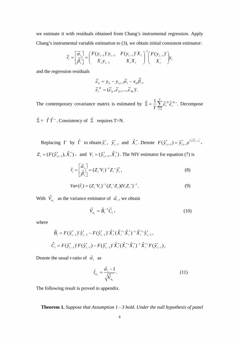
we estimate it with residuals obtained from Chang’s instrumental regression. Apply

Chang’s instrumental variable estimation to (3), we obtain initial consistent estimator:

ii

i

iiii

iiii

i

ii y

XyF

XXyXXyFyyF

r ⎟⎟⎠

⎞⎜⎜⎝

⎛⎟⎟⎠

⎞⎜⎜⎝

⎛=⎥

⎦

⎤⎢⎣

⎡= −

−

−

−−−'

1,1

'1,

'1,1,1, )'()'()'(

~~

~βα

and the regression residuals

)'.~,...,~,~(~,~~~

21

1,

NtttN

t

iititiitit xyy

εεεε

βαε

=

−−= −

The contemporary covariance matrix is estimated by ∑=

=ΣT

t

Nt

NtT 1

'~~1ˆ εε . Decompose

= . Consistency of requires T>N. Σ 'ˆˆ ΓΓ Σ

Replacing by to obtain , and . Denote Γ Γ *ˆ iy *1,ˆ −iy *ˆ

iX*

1,ˆ*1,

*1, ˆ)ˆ( −

−− = tii yctiti eyyF ，

，and . The NIV estimator for equation (7) is )ˆ),ˆ(( **1, itii XyFZ −= )ˆ,ˆ( **

1, itii XyV −=

*1 ˆ')'(ˆˆ

ˆ iiiii

ii yZVZr −=⎥

⎦

⎤⎢⎣

⎡=

βα

, (8)

11 )')('()'()ˆ( −−= iiiiiii ZVZZVZrVar . (9)

With as the variance estimator of i

Vα iα , we obtain

ii CBVi

ˆˆˆ 2−=α ， (10)

where

, *1,

*1****1,

*1,

*1, ˆ'ˆ)ˆ'ˆ(ˆ)'ˆ(ˆ)'ˆ(ˆ

−−

−−− −= iiiiiiiii yXXXXyFyyFB

)ˆ('ˆ)ˆ'ˆ(ˆ)'ˆ()ˆ()'ˆ(ˆ *1,

*1****1,

*1,

*1, −

−−−− −= iiiiiiiii yFXXXXyFyFyFC ,

Denote the usual t-ratio of iα as

i

i

Vt i

α

αα

ˆ1ˆˆ −

= . (11)

The following result is proved in appendix.

Theorem 1. Suppose that Assumption 1 - 3 hold. Under the null hypothesis of panel

8

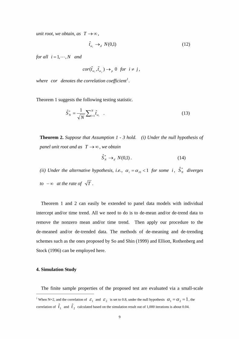
unit root, we obtain, as , ∞→T

(12) )1,0(ˆ Nt di→α

for all and 1, ,i = N

for 0)ˆ,ˆ( pjittcor →αα ji ≠ ,

where cor denotes the correlation coefficient1.

Theorem 1 suggests the following testing statistic.

∑ ==

N

iN it

NS

1* ˆ1ˆ

α . (13)

Theorem 2. Suppose that Assumption 1 - 3 hold. (i) Under the null hypothesis of

panel unit root and as , we obtain ∞→T

)1,0(ˆ* NS dN → . (14)

(ii) Under the alternative hypothesis, i.e., 10 <= ii αα for some , diverges

to at the rate of

i *ˆNS

∞− T .

Theorem 1 and 2 can easily be extended to panel data models with individual

intercept and/or time trend. All we need to do is to de-mean and/or de-trend data to

remove the nonzero mean and/or time trend. Then apply our procedure to the

de-meaned and/or de-trended data. The methods of de-meaning and de-trending

schemes such as the ones proposed by So and Shin (1999) and Elliott, Rothenberg and

Stock (1996) can be employed here.

4. Simulation Study

The finite sample properties of the proposed test are evaluated via a small-scale 1 When N=2, and the correlation of 1ε and 2ε is set to 0.8, under the null hypothesis 121 ==αα , the

correlation of and calculated based on the simulation result out of 1,000 iterations is about 0.04. 1t 2t

9

simulation study. The proposed test is also compared to the other alternative tests such

as the SN test proposed by Chang (2002), CIPS test proposed by Pesaran (2003), and

LLC test proposed by Levin, Lin and Chu (2002).

4.1. Choice of the Nonlinear Instrument Generating Function

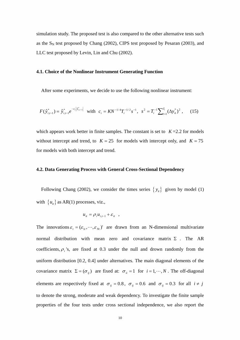
After some experiments, we decide to use the following nonlinear instrument:

*

1,ˆ*1,

*1, ˆ)ˆ( −−

−− = tii yctiti eyyF with , 12/14/1 −−−= sTKNc ii ∑=

− Δ= iT

t iti yTs1

2*12 )( , (15)

which appears work better in finite samples. The constant is set to K =2.2 for models

without intercept and trend, to 25=K for models with intercept only, and

for models with both intercept and trend.

75=K

4.2. Data Generating Process with General Cross-Sectional Dependency

Following Chang (2002), we consider the times series { }ity given by model (1)

with { }itu as AR(1) processes, viz.,

ittiiit uu ερ += −1, ,

The innovations )',,( 1 Nttt εεε = are drawn from an N-dimensional multivariate

normal distribution with mean zero and covariance matrix . The AR

coefficients,

Σ

iρ 's, are fixed at 0.3 under the null and drown randomly from the

uniform distribution [0.2, 0.4] under alternatives. The main diagonal elements of the

covariance matrix )( ijσ=Σ are fixed at: 1=iiσ for Ni ,,1= . The off-diagonal

elements are respectively fixed at 8.0=ijσ , 6.0=ijσ and 3.0=ijσ for all ji ≠

to denote the strong, moderate and weak dependency. To investigate the finite sample

properties of the four tests under cross sectional independence, we also report the

10

simulation result for 0=ijσ for all ji ≠ .

When deterministic components are allowed, we draw the intercept iμ and

coefficient on the linear trend iδ randomly from the uniform distribution, i.e., iμ

and iδ ~Uniform [0.2,0.4].

The coefficient on the lagged dependent variable is fixed at 1== αα i for all

in the case of evaluating the size of the tests, and Ni ,,1= iα is drawn randomly

from the uniform distribution over [0.85, 0.99] in the case of evaluating the power of

the tests. The simulation results that compare our test (SN* ) with Chang test (SN ) are

reported in Table 1~3, where the nominal sizes are set to 0.01, 0.05 and 0.10. The

simulation results that compare our test with CIPS and LLC test are reported in Table

4, where the nominal sizes are set to 0.01, 0.05 and 0.10.

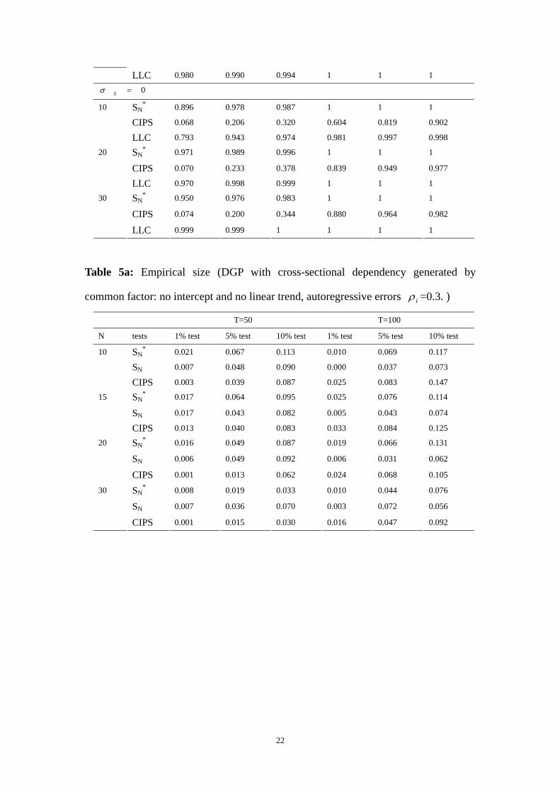
4.3. Data Generating Process with Common Factor

To evaluate how our test performs relative to other tests when the cross sectional

dependence is indeed characterized by some common factors, we consider the DGP

given by Pesaran (2003):

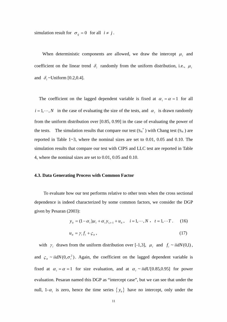
ittiiiiit uyy ++−= −1,)1( αμα , 1, ,i N= ， Tt ,1= . (16)

itiiit fu ςγ += , (17)

with iγ drawn from the uniform distribution over [-1,3], iμ and ,

and . Again, the coefficient on the lagged dependent variable is

fixed at

)1,0(~ iidNfi

),0(~ 2iit iidN σς

1== αα i for size evaluation, and at ]95.0,85.0[~ iidUiα for power

evaluation. Pesaran named this DGP as “intercept case”, but we can see that under the

null, 1- iα is zero, hence the time series { }ity have no intercept, only under the

11

heterogeneous alternatives,{ }ity has the intercept 1- iα . Therefore, Pesaran used the

different models for investigating the size and power of CIPS test. To avoid this

problem, we generate the panel data { }ity as in (1), and in which the disturbances

{ }itu are generated as in (17) to introducing the effect of common factor. The

simulation results that compare our test with Chang test and CIPS test are reported in

Table 5.

4.4. Findings

Our major findings are summarized as follows:

(a). General cross sectional dependence: The empirical sizes of our test in all cases are

fairly close to the nominal sizes. The empirical sizes of Chang test are generally

distorted and the distortions are more pronounced when the cross sectional

dependence is high (e.g., 06 and 0.8). The empirical sizes of CIPS test are somewhere

between the sizes of our test and the sizes of Chang test but closer to the sizes of our

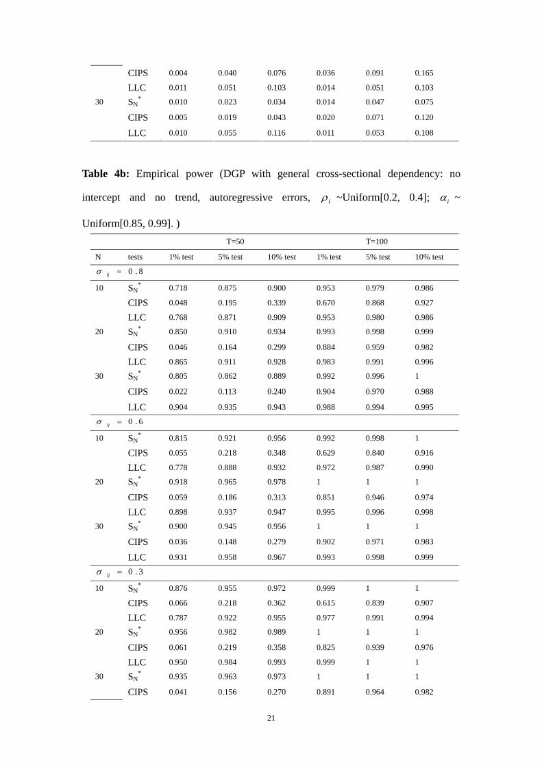
test. Our test has reasonably good power in all designs and the power increases as N

and T increase. The power of CIPS and Chang test are uniformly lower than the

power of our test in all cases.

When intercept is included and N is small, our test has mild size distortion and its

power decreases slightly. When a linear time trend term is included, our test has more

pronounced size distortion and the power decreases significantly. In both cases, our

test performs better than Chang test.

(b). Common factor dependence: The empirical sizes of three tests reported in Table 5

are almost identical and close to the nominal sizes, with the exception for the case:

T=50 and N=30. In this case, our test and CIPS test all have significant size

distortions. The power of our test and Chang test are much higher than the power of

12

CIPS test in all designs.

(c). Cross sectional independence: The LLC test and our test are quite similar in terms

of empirical size and power. But when cross dependence presents, LLC test suffers

from severe over-size problem, and its power is generally lower than the power of our

test.

To summarize, the simulation results show that our test generally performs better than

the alternatives in almost all cases and designs.

5. Conclusion

This paper proposes a panel unit root test that generalizes the nonlinear IV test

proposed by Chang (2002). The generalization is a two-step procedure. In the first

step, Chang’s nonlinear IV estimation is applied to obtain consistent estimate of the

residuals. The residuals are then used to estimate the cross sectional covariance matrix.

In the second step, the data are weighted with the estimated covariance matrix to

eliminated the cross sectional dependence. Chang’s nonlinear IV test is applied to the

weighted data. The resulting test statistic is shown to have limiting standard normal

distributions. Simulation study shows that our test compares favorably to the other

alternative tests.

13

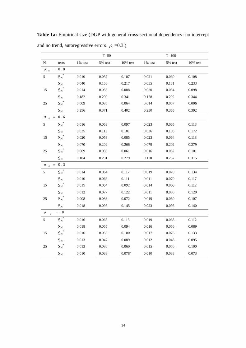
Table 1a: Empirical size (DGP with general cross-sectional dependency: no intercept

and no trend, autoregressive errors iρ =0.3.)

T=50 T=100

N tests 1% test 5% test 10% test 1% test 5% test 10% test

8.0=ijσ

SN* 0.010 0.057 0.107 0.021 0.060 0.108 5

SN 0.040 0.158 0.217 0.055 0.181 0.233

SN* 0.014 0.056 0.088 0.020 0.054 0.098 15

SN 0.182 0.290 0.341 0.178 0.292 0.344

SN* 0.009 0.035 0.064 0.014 0.057 0.096 25

SN 0.256 0.371 0.402 0.250 0.355 0.392

6.0=ijσ

SN* 0.016 0.053 0.097 0.023 0.065 0.118 5

SN 0.025 0.111 0.181 0.026 0.108 0.172

SN* 0.020 0.053 0.085 0.023 0.064 0.118 15

SN 0.070 0.202 0.266 0.079 0.202 0.279

SN* 0.009 0.035 0.061 0.016 0.052 0.101 25

SN 0.104 0.231 0.279 0.118 0.257 0.315

3.0=ijσ

SN* 0.014 0.064 0.117 0.019 0.070 0.134 5

SN 0.010 0.066 0.111 0.011 0.070 0.117

SN* 0.015 0.054 0.092 0.014 0.068 0.112 15

SN 0.012 0.077 0.122 0.011 0.080 0.120

SN* 0.008 0.036 0.072 0.019 0.060 0.107 25

SN 0.018 0.095 0.145 0.023 0.095 0.140

0=ijσ

SN* 0.016 0.066 0.115 0.019 0.068 0.112 5

SN 0.018 0.055 0.094 0.016 0.056 0.089

SN* 0.016 0.056 0.100 0.017 0.076 0.133 15

SN 0.013 0.047 0.089 0.012 0.048 0.095

SN* 0.013 0.036 0.060 0.015 0.056 0.100 25

SN 0.010 0.038 0.078` 0.010 0.038 0.073

14

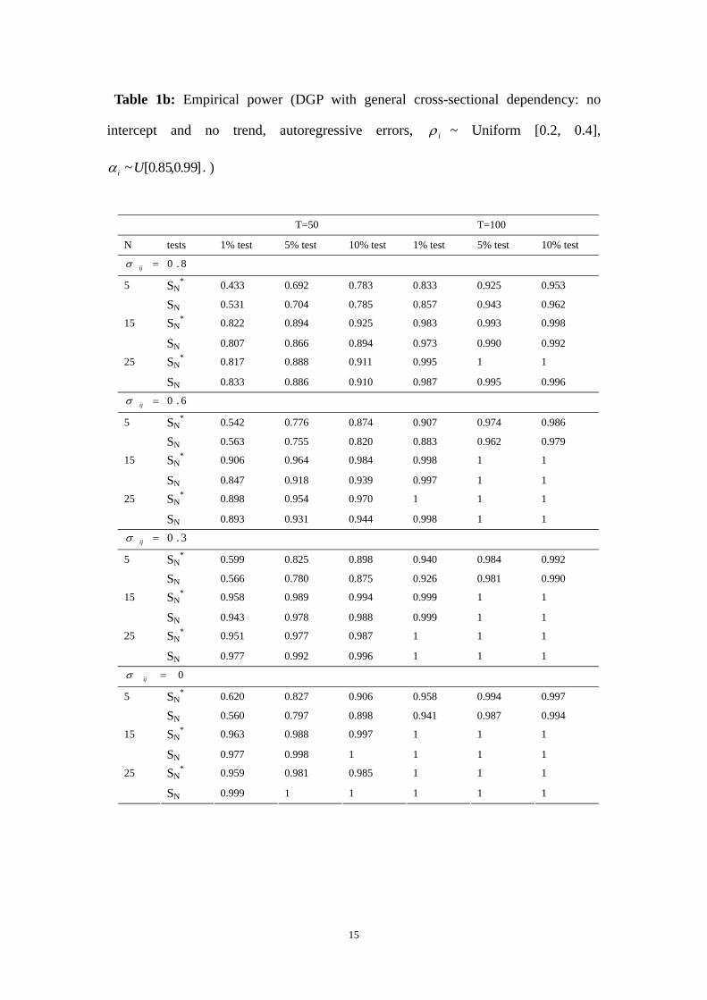
Table 1b: Empirical power (DGP with general cross-sectional dependency: no

intercept and no trend, autoregressive errors, iρ ~ Uniform [0.2, 0.4],

]99.0,85.0[~Uiα .)

T=50 T=100

N tests 1% test 5% test 10% test 1% test 5% test 10% test

8.0=ijσ

SN* 0.433 0.692 0.783 0.833 0.925 0.953 5

SN 0.531 0.704 0.785 0.857 0.943 0.962

SN* 0.822 0.894 0.925 0.983 0.993 0.998 15

SN 0.807 0.866 0.894 0.973 0.990 0.992

SN* 0.817 0.888 0.911 0.995 1 1 25

SN 0.833 0.886 0.910 0.987 0.995 0.996

6.0=ijσ

SN* 0.542 0.776 0.874 0.907 0.974 0.986 5

SN 0.563 0.755 0.820 0.883 0.962 0.979

SN* 0.906 0.964 0.984 0.998 1 1 15

SN 0.847 0.918 0.939 0.997 1 1

SN* 0.898 0.954 0.970 1 1 1 25

SN 0.893 0.931 0.944 0.998 1 1

3.0=ijσ

SN* 0.599 0.825 0.898 0.940 0.984 0.992 5

SN 0.566 0.780 0.875 0.926 0.981 0.990

SN* 0.958 0.989 0.994 0.999 1 1 15

SN 0.943 0.978 0.988 0.999 1 1

SN* 0.951 0.977 0.987 1 1 1 25

SN 0.977 0.992 0.996 1 1 1

0=ijσ

SN* 0.620 0.827 0.906 0.958 0.994 0.997 5

SN 0.560 0.797 0.898 0.941 0.987 0.994

SN* 0.963 0.988 0.997 1 1 1 15

SN 0.977 0.998 1 1 1 1

SN* 0.959 0.981 0.985 1 1 1 25

SN 0.999 1 1 1 1 1

15

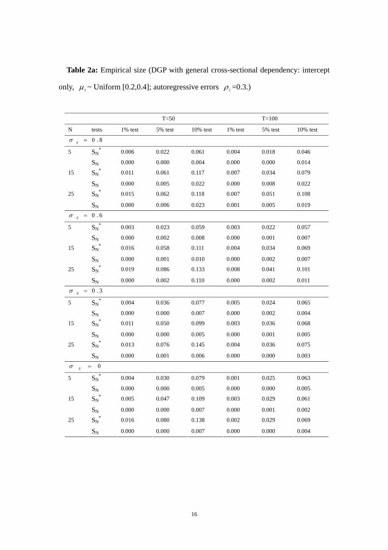
Table 2a: Empirical size (DGP with general cross-sectional dependency: intercept

only, iμ ~ Uniform [0.2,0.4]; autoregressive errors iρ =0.3.)

T=50 T=100

N tests 1% test 5% test 10% test 1% test 5% test 10% test

8.0=ijσ

SN* 0.006 0.022 0.061 0.004 0.018 0.046 5

SN 0.000 0.000 0.004 0.000 0.000 0.014

SN* 0.011 0.061 0.117 0.007 0.034 0.079 15

SN 0.000 0.005 0.022 0.000 0.008 0.022

SN* 0.015 0.062 0.118 0.007 0.051 0.108 25

SN 0.000 0.006 0.023 0.001 0.005 0.019

6.0=ijσ

SN* 0.003 0.023 0.059 0.003 0.022 0.057 5

SN 0.000 0.002 0.008 0.000 0.001 0.007

SN* 0.016 0.058 0.111 0.004 0.034 0.069 15

SN 0.000 0.001 0.010 0.000 0.002 0.007

SN* 0.019 0.086 0.133 0.008 0.041 0.101 25

SN 0.000 0.002 0.110 0.000 0.002 0.011

3.0=ijσ

SN* 0.004 0.036 0.077 0.005 0.024 0.065 5

SN 0.000 0.000 0.007 0.000 0.002 0.004

SN* 0.011 0.050 0.099 0.003 0.036 0.068 15

SN 0.000 0.000 0.005 0.000 0.001 0.005

SN* 0.013 0.076 0.145 0.004 0.036 0.075 25

SN 0.000 0.001 0.006 0.000 0.000 0.003

0=ijσ

SN* 0.004 0.030 0.079 0.001 0.025 0.063 5

SN 0.000 0.000 0.005 0.000 0.000 0.005

SN* 0.005 0.047 0.109 0.003 0.029 0.061 15

SN 0.000 0.000 0.007 0.000 0.001 0.002

SN* 0.016 0.080 0.138 0.002 0.029 0.069 25

SN 0.000 0.000 0.007 0.000 0.000 0.004

16

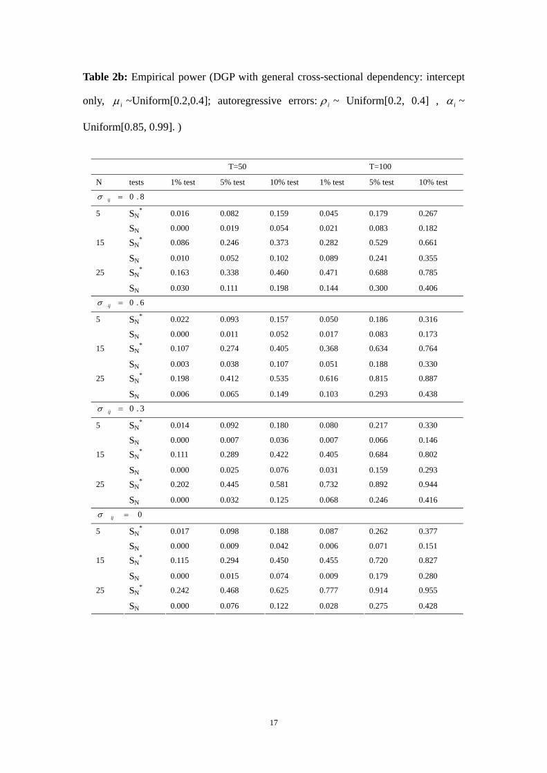
Table 2b: Empirical power (DGP with general cross-sectional dependency: intercept

only, iμ ~Uniform[0.2,0.4]; autoregressive errors: iρ ~ Uniform[0.2, 0.4] , iα ~

Uniform[0.85, 0.99].)

T=50 T=100

N tests 1% test 5% test 10% test 1% test 5% test 10% test

8.0=ijσ

SN* 0.016 0.082 0.159 0.045 0.179 0.267 5

SN 0.000 0.019 0.054 0.021 0.083 0.182

SN* 0.086 0.246 0.373 0.282 0.529 0.661 15

SN 0.010 0.052 0.102 0.089 0.241 0.355

SN* 0.163 0.338 0.460 0.471 0.688 0.785 25

SN 0.030 0.111 0.198 0.144 0.300 0.406

6.0=ijσ

SN* 0.022 0.093 0.157 0.050 0.186 0.316 5

SN 0.000 0.011 0.052 0.017 0.083 0.173

SN* 0.107 0.274 0.405 0.368 0.634 0.764 15

SN 0.003 0.038 0.107 0.051 0.188 0.330

SN* 0.198 0.412 0.535 0.616 0.815 0.887 25

SN 0.006 0.065 0.149 0.103 0.293 0.438

3.0=ijσ

SN* 0.014 0.092 0.180 0.080 0.217 0.330 5

SN 0.000 0.007 0.036 0.007 0.066 0.146

SN* 0.111 0.289 0.422 0.405 0.684 0.802 15

SN 0.000 0.025 0.076 0.031 0.159 0.293

SN* 0.202 0.445 0.581 0.732 0.892 0.944 25

SN 0.000 0.032 0.125 0.068 0.246 0.416

0=ijσ

SN* 0.017 0.098 0.188 0.087 0.262 0.377 5

SN 0.000 0.009 0.042 0.006 0.071 0.151

SN* 0.115 0.294 0.450 0.455 0.720 0.827 15

SN 0.000 0.015 0.074 0.009 0.179 0.280

SN* 0.242 0.468 0.625 0.777 0.914 0.955 25

SN 0.000 0.076 0.122 0.028 0.275 0.428

17

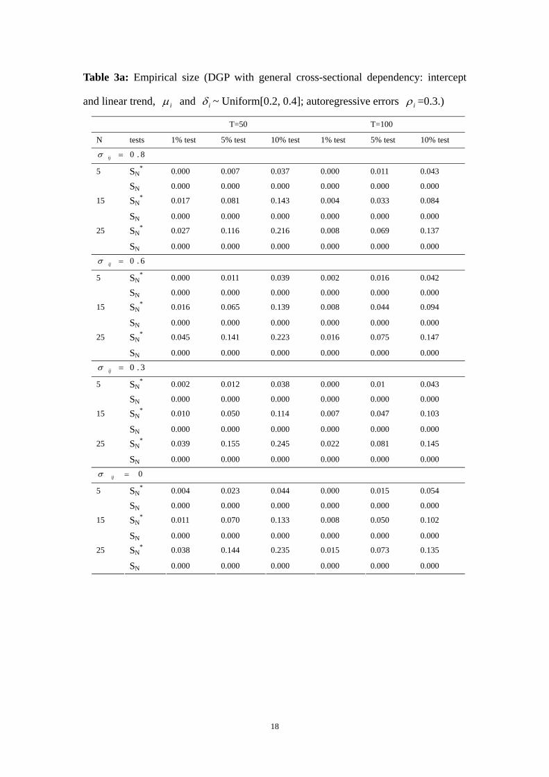
Table 3a: Empirical size (DGP with general cross-sectional dependency: intercept

and linear trend, iμ and iδ ~ Uniform[0.2, 0.4]; autoregressive errors iρ =0.3.)

T=50 T=100

N tests 1% test 5% test 10% test 1% test 5% test 10% test

8.0=ijσ

SN* 0.000 0.007 0.037 0.000 0.011 0.043 5

SN 0.000 0.000 0.000 0.000 0.000 0.000

SN* 0.017 0.081 0.143 0.004 0.033 0.084 15

SN 0.000 0.000 0.000 0.000 0.000 0.000

SN* 0.027 0.116 0.216 0.008 0.069 0.137 25

SN 0.000 0.000 0.000 0.000 0.000 0.000

6.0=ijσ

SN* 0.000 0.011 0.039 0.002 0.016 0.042 5

SN 0.000 0.000 0.000 0.000 0.000 0.000

SN* 0.016 0.065 0.139 0.008 0.044 0.094 15

SN 0.000 0.000 0.000 0.000 0.000 0.000

SN* 0.045 0.141 0.223 0.016 0.075 0.147 25

SN 0.000 0.000 0.000 0.000 0.000 0.000

3.0=ijσ

SN* 0.002 0.012 0.038 0.000 0.01 0.043 5

SN 0.000 0.000 0.000 0.000 0.000 0.000

SN* 0.010 0.050 0.114 0.007 0.047 0.103 15

SN 0.000 0.000 0.000 0.000 0.000 0.000

SN* 0.039 0.155 0.245 0.022 0.081 0.145 25

SN 0.000 0.000 0.000 0.000 0.000 0.000

0=ijσ

SN* 0.004 0.023 0.044 0.000 0.015 0.054 5

SN 0.000 0.000 0.000 0.000 0.000 0.000

SN* 0.011 0.070 0.133 0.008 0.050 0.102 15

SN 0.000 0.000 0.000 0.000 0.000 0.000

SN* 0.038 0.144 0.235 0.015 0.073 0.135 25

SN 0.000 0.000 0.000 0.000 0.000 0.000

18

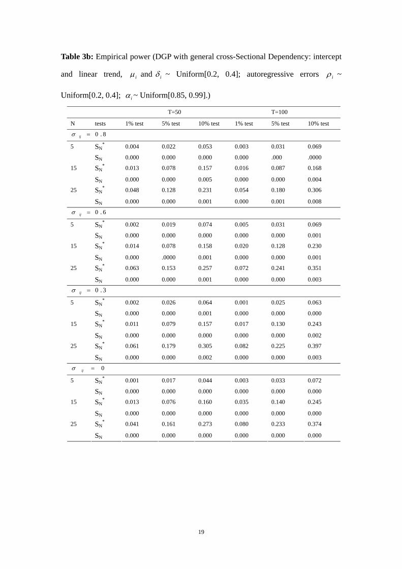
Table 3b: Empirical power (DGP with general cross-Sectional Dependency: intercept

and linear trend, iμ and iδ ~ Uniform[0.2, 0.4]; autoregressive errors iρ ~

Uniform[0.2, 0.4]; iα ~ Uniform[0.85, 0.99].)

T=50 T=100

N tests 1% test 5% test 10% test 1% test 5% test 10% test

8.0=ijσ

SN* 0.004 0.022 0.053 0.003 0.031 0.069 5

SN 0.000 0.000 0.000 0.000 .000 .0000

SN* 0.013 0.078 0.157 0.016 0.087 0.168 15

SN 0.000 0.000 0.005 0.000 0.000 0.004

SN* 0.048 0.128 0.231 0.054 0.180 0.306 25

SN 0.000 0.000 0.001 0.000 0.001 0.008

6.0=ijσ

SN* 0.002 0.019 0.074 0.005 0.031 0.069 5

SN 0.000 0.000 0.000 0.000 0.000 0.001

SN* 0.014 0.078 0.158 0.020 0.128 0.230 15

SN 0.000 .0000 0.001 0.000 0.000 0.001

SN* 0.063 0.153 0.257 0.072 0.241 0.351 25

SN 0.000 0.000 0.001 0.000 0.000 0.003

3.0=ijσ

SN* 0.002 0.026 0.064 0.001 0.025 0.063 5

SN 0.000 0.000 0.001 0.000 0.000 0.000

SN* 0.011 0.079 0.157 0.017 0.130 0.243 15

SN 0.000 0.000 0.000 0.000 0.000 0.002

SN* 0.061 0.179 0.305 0.082 0.225 0.397 25

SN 0.000 0.000 0.002 0.000 0.000 0.003

0=ijσ

SN* 0.001 0.017 0.044 0.003 0.033 0.072 5

SN 0.000 0.000 0.000 0.000 0.000 0.000

SN* 0.013 0.076 0.160 0.035 0.140 0.245 15

SN 0.000 0.000 0.000 0.000 0.000 0.000

SN* 0.041 0.161 0.273 0.080 0.233 0.374 25

SN 0.000 0.000 0.000 0.000 0.000 0.000

19

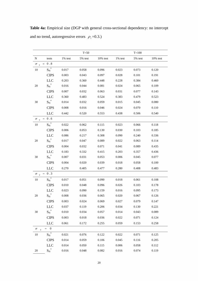
Table 4a: Empirical size (DGP with general cross-sectional dependency: no intercept

and no trend, autoregressive errors iρ =0.3.)

T=50 T=100

N tests 1% test 5% test 10% test 1% test 5% test 10% test

8.0=ijσ

SN* 0.017 0.058 0.096 0.023 0.073 0.120

CIPS 0.003 0.043 0.097 0.028 0.101 0.191

10

LLC 0.203 0.360 0.448 0.228 0.384 0.460

SN* 0.016 0.044 0.081 0.024 0.065 0.109

CIPS 0.007 0.032 0.063 0.031 0.077 0.143

20

LLC 0.360 0.483 0.524 0.383 0.479 0.523

SN* 0.014 0.032 0.059 0.015 0.045 0.080

CIPS 0.008 0.016 0.046 0.024 0.070 0.110

30

LLC 0.442 0.520 0.553 0.438 0.506 0.540

6.0=ijσ

SN* 0.022 0.062 0.115 0.023 0.066 0.118

CIPS 0.006 0.053 0.130 0.030 0.103 0.185

10

LLC 0.086 0.217 0.308 0.090 0.240 0.336

SN* 0.017 0.047 0.089 0.022 0.063 0.114

CIPS 0.004 0.032 0.071 0.041 0.089 0.435

20

LLC 0.183 0.332 0.415 0.203 0.357 0.436

SN* 0.007 0.031 0.053 0.006 0.045 0.077

CIPS 0.004 0.020 0.039 0.018 0.058 0.100

30

LLC 0.270 0.405 0.477 0.280 0.408 0.483

3.0=ijσ

SN* 0.017 0.051 0.090 0.018 0.061 0.108

CIPS 0.010 0.048 0.096 0.026 0.103 0.178

10

LLC 0.023 0.090 0.159 0.016 0.095 0.173

SN* 0.008 0.036 0.065 0.020 0.067 0.126

CIPS 0.003 0.024 0.069 0.027 0.079 0.147

20

LLC 0.037 0.119 0.206 0.034 0.130 0.221

SN* 0.010 0.034 0.057 0.014 0.043 0.089

CIPS 0.003 0.018 0.036 0.022 0.071 0.124

30

LLC 0.061 0.172 0.255 0.059 0.153 0.258

0=ijσ

SN* 0.021 0.076 0.122 0.022 0.071 0.125

CIPS 0.014 0.059 0.106 0.045 0.116 0.205

10

LLC 0.014 0.050 0.115 0.006 0.058 0.112

20 SN* 0.016 0.048 0.082 0.016 0.074 0.119

20

CIPS 0.004 0.040 0.076 0.036 0.091 0.165

LLC 0.011 0.051 0.103 0.014 0.051 0.103

SN* 0.010 0.023 0.034 0.014 0.047 0.075

CIPS 0.005 0.019 0.043 0.020 0.071 0.120

30

LLC 0.010 0.055 0.116 0.011 0.053 0.108

Table 4b: Empirical power (DGP with general cross-sectional dependency: no

intercept and no trend, autoregressive errors, iρ ~Uniform[0.2, 0.4]; iα ~

Uniform[0.85, 0.99].) T=50 T=100

N tests 1% test 5% test 10% test 1% test 5% test 10% test

8.0=ijσ

SN* 0.718 0.875 0.900 0.953 0.979 0.986

CIPS 0.048 0.195 0.339 0.670 0.868 0.927

10

LLC 0.768 0.871 0.909 0.953 0.980 0.986

SN* 0.850 0.910 0.934 0.993 0.998 0.999

CIPS 0.046 0.164 0.299 0.884 0.959 0.982

20

LLC 0.865 0.911 0.928 0.983 0.991 0.996

SN* 0.805 0.862 0.889 0.992 0.996 1

CIPS 0.022 0.113 0.240 0.904 0.970 0.988

30

LLC 0.904 0.935 0.943 0.988 0.994 0.995

6.0=ijσ

SN* 0.815 0.921 0.956 0.992 0.998 1

CIPS 0.055 0.218 0.348 0.629 0.840 0.916

10

LLC 0.778 0.888 0.932 0.972 0.987 0.990

SN* 0.918 0.965 0.978 1 1 1

CIPS 0.059 0.186 0.313 0.851 0.946 0.974

20

LLC 0.898 0.937 0.947 0.995 0.996 0.998

SN* 0.900 0.945 0.956 1 1 1

CIPS 0.036 0.148 0.279 0.902 0.971 0.983

30

LLC 0.931 0.958 0.967 0.993 0.998 0.999

3.0=ijσ

SN* 0.876 0.955 0.972 0.999 1 1

CIPS 0.066 0.218 0.362 0.615 0.839 0.907

10

LLC 0.787 0.922 0.955 0.977 0.991 0.994

SN* 0.956 0.982 0.989 1 1 1

CIPS 0.061 0.219 0.358 0.825 0.939 0.976

20

LLC 0.950 0.984 0.993 0.999 1 1

SN* 0.935 0.963 0.973 1 1 1 30

CIPS 0.041 0.156 0.270 0.891 0.964 0.982

21

LLC 0.980 0.990 0.994 1 1 1

0=ijσ

SN* 0.896 0.978 0.987 1 1 1

CIPS 0.068 0.206 0.320 0.604 0.819 0.902

10

LLC 0.793 0.943 0.974 0.981 0.997 0.998

SN* 0.971 0.989 0.996 1 1 1

CIPS 0.070 0.233 0.378 0.839 0.949 0.977

20

LLC 0.970 0.998 0.999 1 1 1

SN* 0.950 0.976 0.983 1 1 1

CIPS 0.074 0.200 0.344 0.880 0.964 0.982

30

LLC 0.999 0.999 1 1 1 1

Table 5a: Empirical size (DGP with cross-sectional dependency generated by

common factor: no intercept and no linear trend, autoregressive errors iρ =0.3. )

T=50 T=100

N tests 1% test 5% test 10% test 1% test 5% test 10% test

SN* 0.021 0.067 0.113 0.010 0.069 0.117

SN 0.007 0.048 0.090 0.000 0.037 0.073

10

CIPS 0.003 0.039 0.087 0.025 0.083 0.147

SN* 0.017 0.064 0.095 0.025 0.076 0.114

SN 0.017 0.043 0.082 0.005 0.043 0.074

15

CIPS 0.013 0.040 0.083 0.033 0.084 0.125

SN* 0.016 0.049 0.087 0.019 0.066 0.131

SN 0.006 0.049 0.092 0.006 0.031 0.062

20

CIPS 0.001 0.013 0.062 0.024 0.068 0.105

SN* 0.008 0.019 0.033 0.010 0.044 0.076

SN 0.007 0.036 0.070 0.003 0.072 0.056

30

CIPS 0.001 0.015 0.030 0.016 0.047 0.092

22

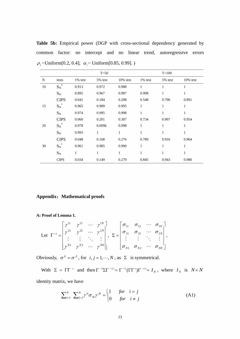
Table 5b: Empirical power (DGP with cross-sectional dependency generated by

common factor: no intercept and no linear trend, autoregressive errors

iρ ~Uniform[0.2, 0.4]; iα ~ Uniform[0.85, 0.99].)

T=50 T=100

N tests 1% test 5% test 10% test 1% test 5% test 10% test

SN* 0.913 0.972 0.988 1 1 1

SN 0.895 0.967 0.987 0.998 1 1

10

CIPS 0.041 0.184 0.298 0.548 0.796 0.891

SN* 0.965 0.989 0.995 1 1 1

SN 0.974 0.995 0.998 1 1 1

15

CIPS 0.060 0.201 0.307 0.734 0.907 0.954

SN* 0.978 0.0096 0.998 1 1 1

SN 0.993 1 1 1 1 1

20

CIPS 0.048 0.168 0.276 0.789 0.916 0.964

SN* 0.961 0.985 0.990 1 1 1

SN 1 1 1 1 1 1

30

CIPS 0.034 0.149 0.279 0.845 0.943 0.980

Appendix：Mathematical proofs

A: Proof of Lemma 1.

Let , ,

⎥⎥⎥⎥⎥

⎦

⎤

⎢⎢⎢⎢⎢

⎣

⎡

=Γ−

NNNN

N

N

γγγ

γγγγγγ

21

22221

11211

1

⎥⎥⎥⎥

⎦

⎤

⎢⎢⎢⎢

⎣

⎡

=Σ

NNNN

N

N

σσσ

σσσσσσ

21

22221

11211

Obviously, , for , as jiij σσ = Nji ,,1, = Σ is symmetrical.

With and then , where is

identity matrix, we have

'ΓΓ=Σ NI=ΓΓΓΓ=ΣΓΓ −−−− ')'(' 1111NI NN ×

(A1) ⎩⎨⎧

≠=

=∑∑ == jiforjiforN

kjk

skisN

s 01

11γσγ

23

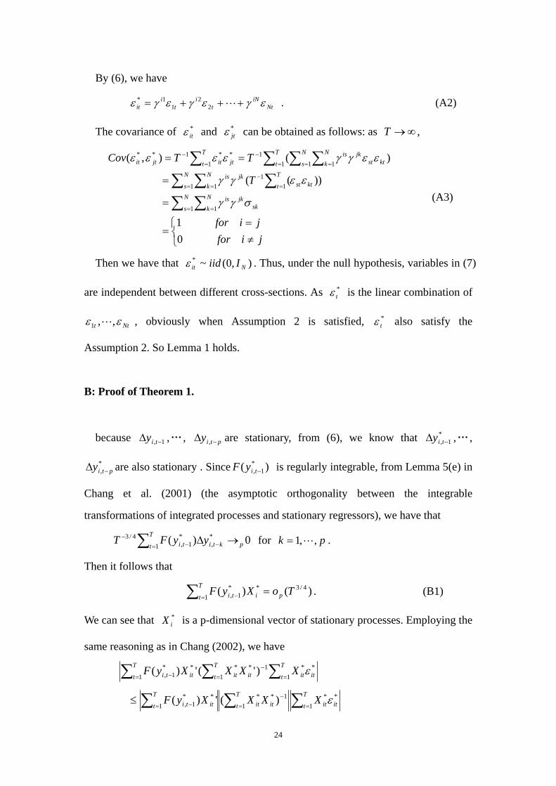
By (6), we have

. (A2) NtiN

ti

ti

it εγεγεγε +++= 22

11*

The covariance of and can be obtained as follows: as , *itε *

jtε ∞→T

⎩⎨⎧

≠=

=

=

=

==

∑ ∑∑ ∑ ∑

∑ ∑ ∑∑

= =

= = =−

= = ==−−

jiforjifor

T

TTCov

N

s

N

k skjkis

ktstN

s

N

k

T

tjkis

T

t

N

s

N

k ktstjkisT

tjtitjtit

01

))((

)(),(

1 1

1 1 11

1 1 111**1**

σγγ

εεγγ

εεγγεεεε

(A3)

Then we have that . Thus, under the null hypothesis, variables in (7)

are independent between different cross-sections. As is the linear combination of

),0(~*Nit Iiidε

*tε

Ntt εε ,,1 , obviously when Assumption 2 is satisfied, also satisfy the

Assumption 2. So Lemma 1 holds.

*tε

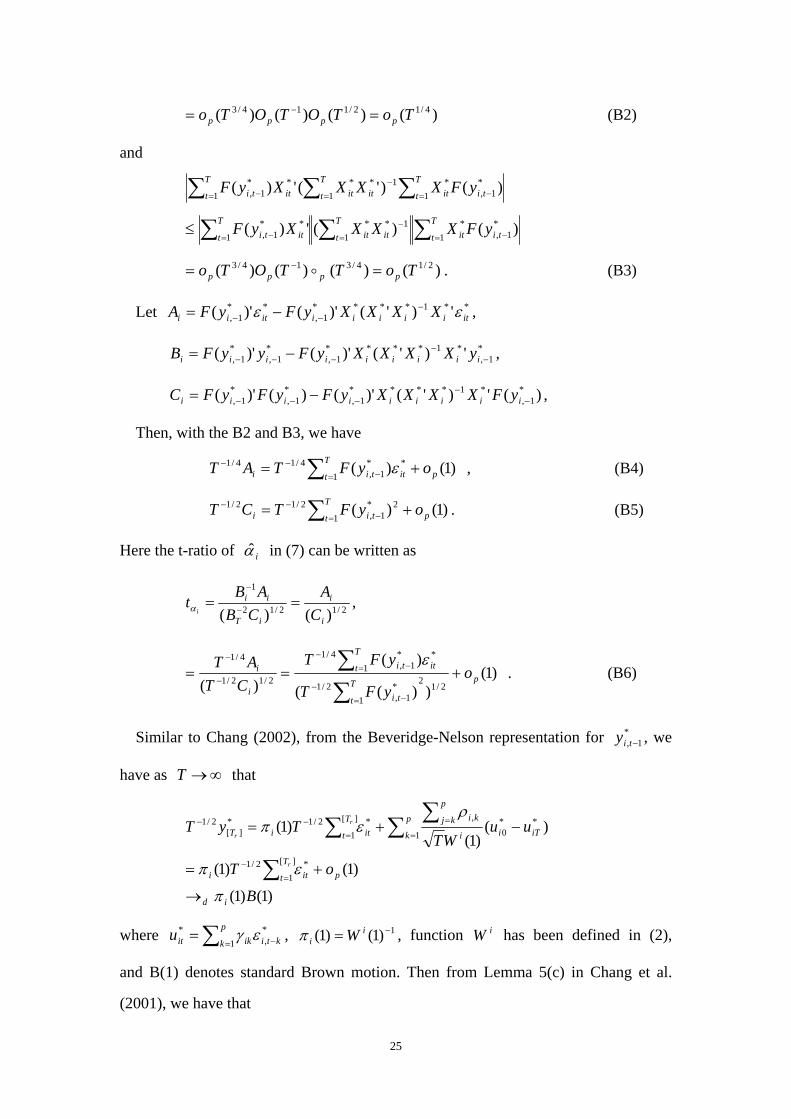
B: Proof of Theorem 1.

because ,… , are stationary, from (6), we know that ,… ,

are also stationary . Since is regularly integrable, from Lemma 5(e) in

Chang et al. (2001) (the asymptotic orthogonality between the integrable

transformations of integrated processes and stationary regressors), we have that

1, −Δ tiy ptiy −Δ ,*

1, −Δ tiy

*, ptiy −Δ )( *

1, −tiyF

for 0)(1

*,

*1,

4/3 ∑= −−− →Δ

T

t pktiti yyFT pk ,,1= .

Then it follows that

)()( 4/3*1

*1, ToXyF pi

T

t ti =∑ = − . (B1)

We can see that is a p-dimensional vector of stationary processes. Employing the

same reasoning as in Chang (2002), we have

*iX

∑ ∑ ∑= =−

−T

t

T

t

T

t itititititti XXXXyF1 1

**1****1, )'(')( ε

=1

∑∑∑ ==−

= −≤T

t ititT

t ititT

t itti XXXXyF1

**1

1**1

**1, )(')( ε

24

)()()()( 4/12/114/3 ToTOTOTo pppp == − (B2)

and

∑ ∑ ∑= = = −−

−T

t

T

t

T

t tiititititti yFXXXXyF1 1 1

*1,

*1****1, )()'(')(

∑∑∑ = −=−

= −≤T

t tiitT

t ititT

t itti yFXXXXyF1

*1,

*1

1**1

**1, )()(')(

)()()()( 2/14/314/3 ToTTOTo pppp == − . (B3)

Let , **1****1,

**1, ')'()'()'( itiiiiiitii XXXXyFyFA εε −

−− −=

*1,

*1****1,

*1,

*1, ')'()'()'( −

−−−− −= iiiiiiiii yXXXXyFyyFB ,

)(')'()'()()'( *1,

*1****1,

*1,

*1, −

−−−− −= iiiiiiiii yFXXXXyFyFyFC ,

Then, with the B2 and B3, we have

, (B4) )1()(1

**1,

4/14/1p

T

t ittii oyFTAT += ∑ = −−− ε

. (B5) )1()(1

2*1,

2/12/1p

T

t tii oyFTCT += ∑ = −−−

Here the t-ratio of iα in (7) can be written as

2/12/12

1

)()( i

i

iT

ii

CA

CBABt

i== −

−

α ,

)1())((

)()( 2/12

1*

1,2/1

1**

1,4/1

2/12/1

4/1

pT

t ti

T

t itti

i

i oyFT

yFTCT

AT+==

∑∑

= −−

= −−

−

− ε . (B6)

Similar to Chang (2002), from the Beveridge-Nelson representation for , we

have as that

*1, −tiy

∞→T

)1()1(

)1()1(

)()1(

)1(

][

1*2/1

][

1 1**

0,*2/1*

][2/1

B

oT

uuWT

TyT

id

T

t piti

T

t

p

k iTii

p

kj kiitiT

r

r

r

π

επ

ρεπ

→

+=

−+=

∑

∑ ∑∑

=−

= =

=−−

where , , function has been defined in (2),

and B(1) denotes standard Brown motion. Then from Lemma 5(c) in Chang et al.

(2001), we have that

*,1

*kti

p

k ikitu −=∑= εγ 1)1()1( −= ii Wπ iW

25

∑ ∫=

∞

∞−−− ⎟

⎠⎞⎜

⎝⎛→

T

t iiditti BdssFLyFT1

2/12**

1,4/1 )1())1(()0,1()( πε , (B7)

From Lemma 5(i) in Chang et al. (2001), we have that

, (B8) ∑ ∫=

∞

∞−−− →

T

t iidti dssFLyFT1

22*1,

2/1 ))1(()0,1()( π

where ∫ <−=→

t

i drsrFstL00

})({121lim),( δδδ

,is the local time of F--the time that F

spends in the neighborhood of , up to , measured in chronological units. Using

the results in (B7) and (B8) to (B6), we have the result immediately that

s t

)1())1(()0,1(

)1())1(()0,1(2/1

2

2/12

BdssFL

BdssFLt

ii

ii

di=

⎟⎠⎞⎜

⎝⎛

⎟⎠⎞⎜

⎝⎛

→

∫

∫∞

∞−

∞

∞−

π

πα , (B9)

From result in Lemma 1, we have that, for ji ≠ , as ∞→T ,

0),( **pjicor →εε ,

then it follows from (7) that

0),( **pjtit yycor → .

So we have that , as 0),( piittcor →αα ∞→T . Since the Σ then Γ are the consistent

estimates of and , the Theorem 1 holds. Σ Γ

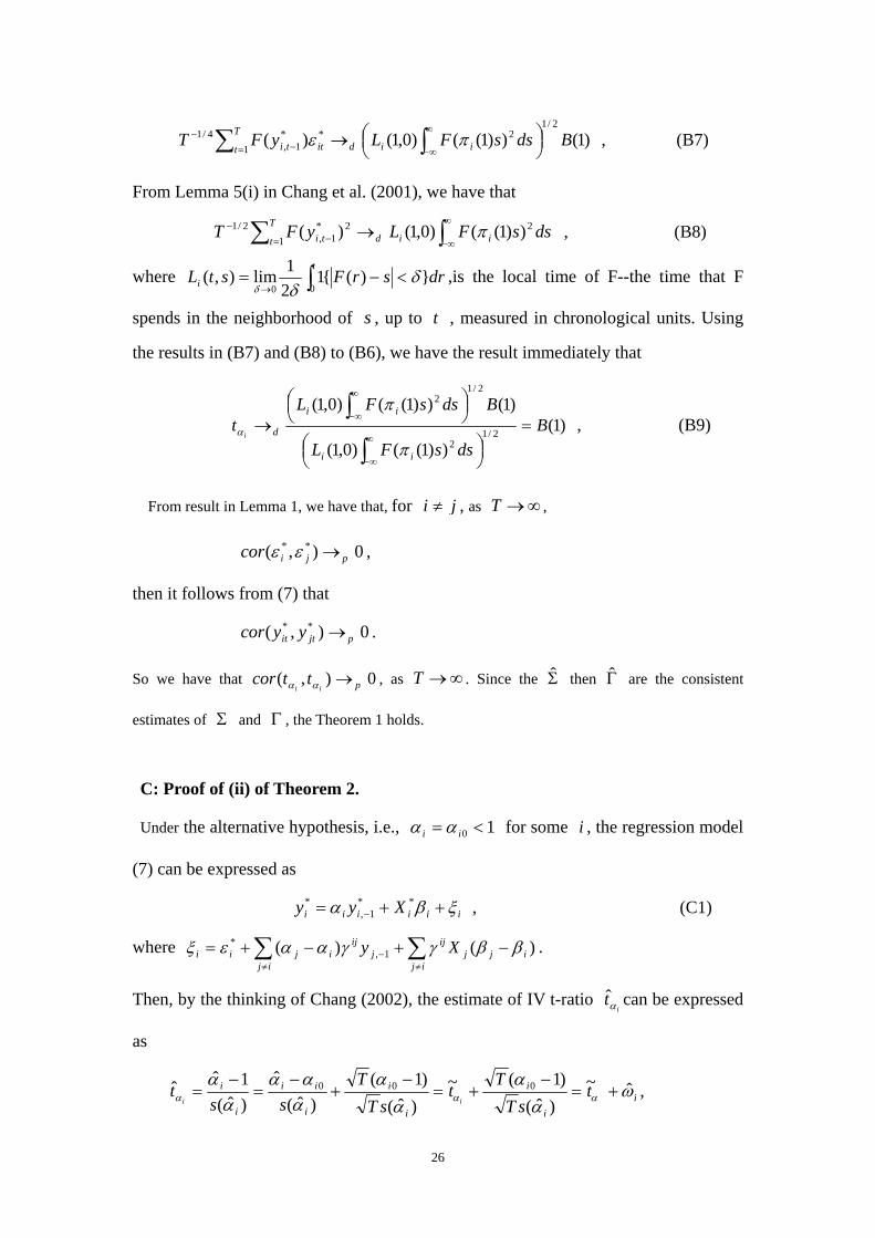
C: Proof of (ii) of Theorem 2.

Under the alternative hypothesis, i.e., 10 <= ii αα for some i , the regression model

(7) can be expressed as

, (C1) iiiiii Xyy ξβα ++= −**

1,*

where ∑∑≠≠

− −+−+=ij

ijjij

ijj

ijijii Xy )()( 1,

* ββγγααεξ .

Then, by the thinking of Chang (2002), the estimate of IV t-ratio can be expressed

as

itα

ii

i

i

i

i

ii

i

i tsT

Tt

sTT

sst

iiω

αα

αα

ααα

αα

ααα ˆ~)ˆ(

)1(~)ˆ(

)1()ˆ(

ˆ)ˆ(1ˆˆ 000 +=

−+=

−+

−=

−= ,

26

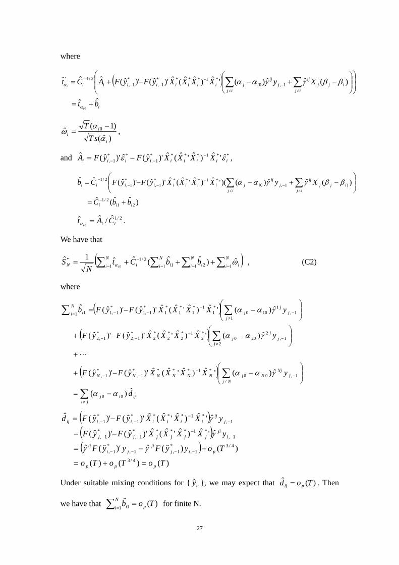
where

( )

i

ij ijijj

ijj

ijijiiiiiiii

bt

XyXXXXyFyFACt

i

i

ˆˆ

)(ˆˆ)('ˆ)ˆˆ(ˆ)'ˆ()'ˆ(ˆˆ~

0

1,0*1****

1,*

1,2/1

+=

⎟⎟⎠

⎞⎜⎜⎝

⎛⎟⎟⎠

⎞⎜⎜⎝

⎛−+−−+= ∑ ∑

≠ ≠−

−−−

−

α

α ββγγαα

)ˆ()1(ˆ 0

i

ii sT

Tα

αω

−= ,

and , **1****1,

**1, ˆ'ˆ)ˆ'ˆ(ˆ)'ˆ(ˆ)'ˆ(ˆ

iiiiiiiii XXXXyFyFA εε −−− −=

)ˆˆ(ˆ

)(ˆˆ)()('ˆ)ˆ'ˆ(ˆ)'ˆ()'ˆ(ˆˆ

212/1

)1,0*1****

1,*

1,2/1

iii

ij ijijj

ijj

ijijiiiiiiii

bbC

XyXXXXyFyFCb

+=

⎟⎟⎠

⎞⎜⎜⎝

⎛−+−−=

−

≠ ≠−

−−−

− ∑ ∑ ββγγαα

. 2/1ˆ/ˆˆ0 ii CAt

i=α

We have that

( )∑ ∑∑ = =−

=+++=

N

i

N

i iN

i iiiN

iN bbCtN

Si 1 1 21

2/11

* ˆ)ˆˆ(ˆˆ1ˆ0

ωα ∑ =1 , (C2)

where

( )

( )

( )

ijji

ij

Njj

NjNjNNNNNN

jj

jj

jj

jj

N

i i

d

yXXXXyFyF

yXXXXyFyF

yXXXXyFyFb

ˆ)(

ˆ)('ˆ)ˆ'ˆ(ˆ)'ˆ()'ˆ(

ˆ)('ˆ)ˆ'ˆ(ˆ)'ˆ()'ˆ(

ˆ)('ˆ)ˆ'ˆ(ˆ)'ˆ()'ˆ(ˆ

00

1,00*1****

1,*

1,

21,

2200

*2

1*2

*2

*2

*1,2

*1,2

11,

1100

*1

1*1

*1

*1

*1,1

*1,11 1

∑

∑

∑

∑∑

≠

≠−

−−−

≠−

−−−

≠−

−−−=

−=

⎟⎟⎠

⎞⎜⎜⎝

⎛−−+

+

⎟⎟⎠

⎞⎜⎜⎝

⎛−−+

⎟⎟⎠

⎞⎜⎜⎝

⎛−−=

αα

γαα

γαα

γαα

( )( )( )

)()()(

)()ˆ(ˆ)'ˆ(ˆ

ˆ'ˆ)ˆ'ˆ(ˆ)'ˆ()'ˆ(

ˆ'ˆ)ˆ'ˆ(ˆ)'ˆ()'ˆ(ˆ

4/3

4/31,

*1,1,

*1,

1,*1****

1,*

1,

1,*1****

1,*

1,

ToToTo

ToyyFyyF

yXXXXyFyF

yXXXXyFyFd

ppp

pijji

jiij

iji

jjjjjj

jij

iiiiiiij

=+=

+−=

−−

−=

−−−−

−−

−−

−−

−−

γγ

γ

γ

Under suitable mixing conditions for { }, we may expect that . Then

we have that for finite N.

ity )(ˆ Tod pij =

)(ˆ1 1 Tob p

N

i i =∑ =

27

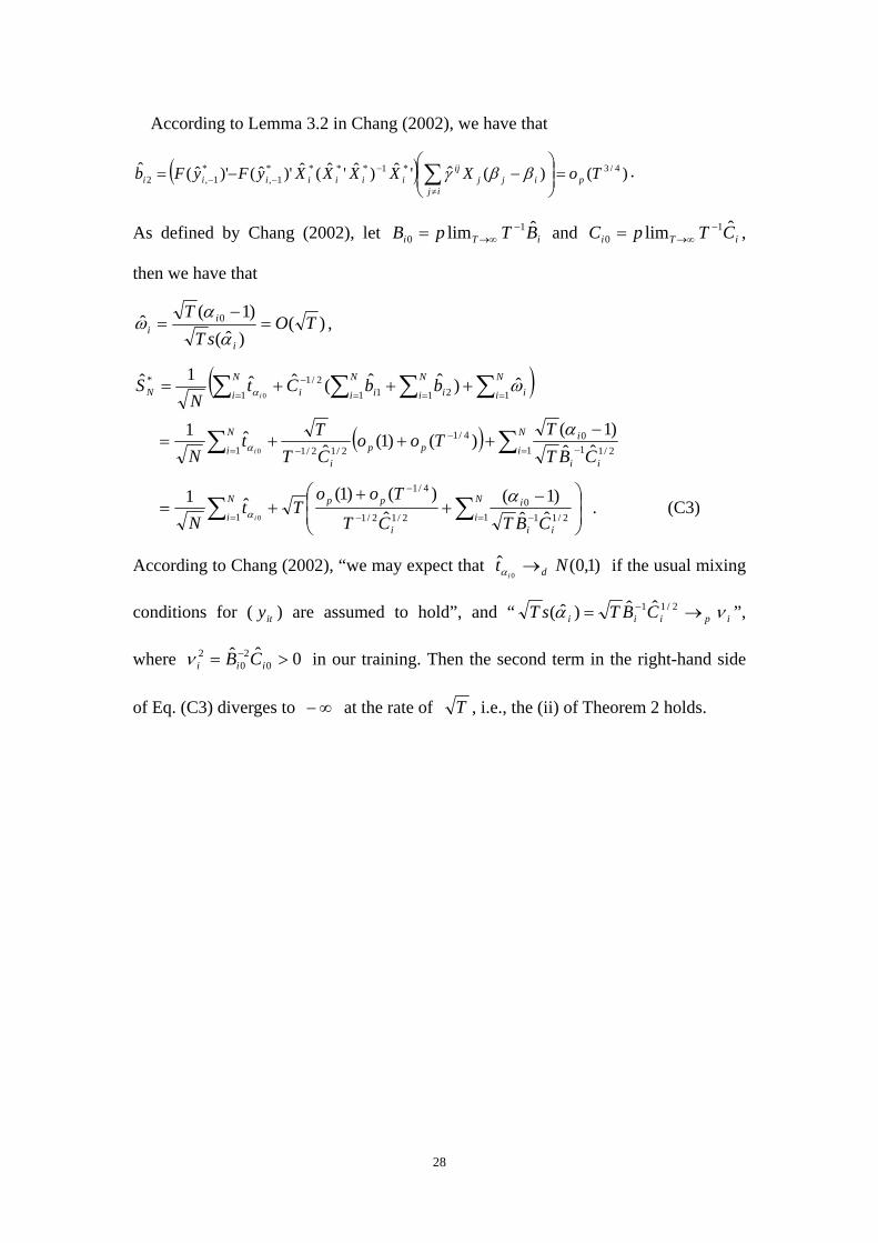
According to Lemma 3.2 in Chang (2002), we have that

( ) )()(ˆ'ˆ)ˆ'ˆ(ˆ)'ˆ()'ˆ(ˆ 4/3*1****1,

*1,2 ToXXXXXyFyFb p

ijijj

ijiiiiiii =⎟⎟

⎠

⎞⎜⎜⎝

⎛−−= ∑

≠

−−− ββγ .

As defined by Chang (2002), let and ,

then we have that

iTi BTpB ˆlim 10

−∞→= iTi CTpC ˆlim 1

0−

∞→=

)()ˆ(

)1(ˆ 0 TOsT

T

i

ii =

−=

αα

ω ,

( )

( )∑ ∑

∑ ∑∑∑

= = −−

−

= ==−

=

−+++=

+++=

N

i

N

iii

ipp

i

N

i

N

i iN

i iiiN

iN

CBTT

TooCTTt

N

bbCtN

S

i

i

1 1 2/1104/1

2/12/1

1 11 212/1

1*

ˆˆ)1(

)()1(ˆˆ1

ˆ)ˆˆ(ˆˆ1ˆ

0

0

α

ω

α

α

∑ ∑= −−

−

⎟⎟⎠

⎞⎜⎜⎝

⎛ −+

++=

N

i

N

iii

i

i

pp

CBTCT

TooTt

N i1 2/110

2/12/1

4/1

ˆˆ)1(

ˆ)()1(ˆ1

0

αα =1

. (C3)

According to Chang (2002), “we may expect that if the usual mixing

conditions for ( ) are assumed to hold”, and “

)1,0(ˆ0

Nt di→α

ity ipiii CBTsT να →= − 2/11 ˆˆ)ˆ( ”,

where 0ˆˆ0

20

2 >= −iii CBν in our training. Then the second term in the right-hand side

of Eq. (C3) diverges to at the rate of ∞− T , i.e., the (ii) of Theorem 2 holds.

28

References

Bai, J. and Ng, S., 2001, A PANIC Attack on Unit Roots and Cointegration, Mimeo,

Boston College, Department of Economics.

Bai, J. and Ng, S., 2004, A PANIC Attack on Unit Roots and Cointegration,

Econometrica, 72(4), 127-1178.

Breitung, J. and Das, S., 2004, Panel Unit Root Tests under Cross Sectional

Dependence, Work paper, University of Bonn, Germany.

Chang, Y., 2002, Nonlinear IV Unit Root Tests in Panels with Cross-sectional

Dependency, Journal of Econometrics, 10,261-292.

Chang, Y., 2004, Bootstrap Unit Root Tests in Panels with Cross-Sectional

Dependency, Journal of Econometrics, 120,263-293.

Chang, Y., J.Y. Park and P.C.B. Phillips, 2001, Nonlinear econometric models with

cointegrated and deterministically trending regressors, Econometrics Journal, 4,

1-36.

Choi, I., 2001, Unit Root Tests for Panel Data, Journal of International Money and

Finance, 20,249-272.

Choi, I., 2002, Combination Unit Root Tests for Cross-Sectional Correlated Panels,

Mimeo, HongKong University of Science and Technology.

Elliott, G., Rothenberg, T. and Stock, J., 1996, Efficient Tests for an Autoregressive

Unit Root, Econometrica, 64,813-836.

Flôres, R., P-Y. Preumont and Szafarz, A., 1995, Multivariate Unit Root Tests,

Mimeo., Universite Libre de Bruxelles, Brussels.

Hadri, K., 2000, Testing for Unit Roots in Heterogeneous Panel Data, Econometrics

Journal, 3,148-161.

Harris, R.D.F. and Tzavalis, E., 1999, Inference for Unit Roots in Dynamic Panels

where The Time Dimension is Fixed, Journal of Econometrics, 91,201-226. 22.

Hurlin, C. and Mignon, V., 2004, Second Generation Panel Unit Root Tests, LEO,

University of Orléans, France.

29

Im, K.S. and Pesaran, M.H., 2003, On the Panel Unit Root Tests Using Nonlinear

Instrumental IV variables, Mimeo, University of Southern California.

Im, K.S., Pesaran, M.H. and Shin, Y., 1997, Testing for Unit Roots in Heterogeneous

Panels, DAE, Working Paper 9526, University of Cambridge.

Im, K.S., Pesaran, M.H. and Shin, Y., 2003, Testing for Unit Roots in Heterogeneous

Panels, Journal of Econometrics,15,1,53-74.

Levin, A. and Lin, C.F., 1992, Unit Root Test in Panel Data: Asymptotic and Finite

Sample Properties, University of California at San Diego, Discussion Paper92-93.

Levin, A. and Lin, C.F., 1993, Unit Root Test in Panel Data: New Results, University

of California at San Diego, Discussion Paper93-56.

Levin, A., Lin, C.F. and Chu, C.S.J., 2002, Unit Root Test in Panel Data: Asymptotic

and Finite Sample Properties, Journal of Econometrics, 108,1-24.

Maddala, G.S. and Wu, S., 1999, A Comparative Study of Unit Root Tests with Panel

Data and a New Simple Test, Oxford Bulletin of Economics and Statistics, special

issue, 631- 652.

Moon, H.R. and Perron, B., 2004, Testing for a Unit Root in Panels with Dynamic

Factors, Journal of Econometrics,12,81-126.

Moon, H.R. and Perron, B., 2004, Asymptotic Local Power of Pooled t-Ratio Tests

for Unit Roots in Panels with Fixed Effects, Mimeo, University of Montréal.

Park, J.Y. and P.C.B. Phillips, 2001, Nonlinear regressions with integrated time series,

Econometrica 69, 1452-1498.

Pesaran, H.M., 2003, A Simple Panel Unit Root Test in the Presence of Cross Section

Dependence, Mimeo, University of Southern California.

Phillips, P.C.B. and Sul, D., 2003, Dynamic Panel Estimation and Homogeneity

Testing Under Cross Section Dependence, Econometrics Journal, 6(1),217-259.

So, B.S. and Shin, D.W., 1999, Recursive Mean Adjustment in Time Series Inferences,

Statistics & Probability Letters, 43,65-73.

Shaman,P. and Stine,.A., 1988, The Bias of Autoregressive Coefficient Estimators.

Journal of the American Statistical Association, 83(3),842-8.

Taylor, M.P. and Sarno, L., 1998, The Behavior of Real Exchange Rates During the Post-Bretton

30

Woods Period, Journal of international Econoimics,46,281-312.

31