THE BRIDGING DOMAIN MULTISCALE METHOD AND ITS HIGH

PERFORMANCE COMPUTING IMPLEMENTATION

Shaoping Xiao

Department of Mechanical and Industrial Engineering

Center for Computer-Aided Design

The University of Iowa, Iowa City, IA 52242

shaoping-xiao@uiowa.edu

Jun Ni

Department of Radiology

Department of Mechanical Engineering

Department of Computer Science

The University of Iowa, Iowa City, IA 52242

jun-ni@uiowa.edu

Shaowen Wang

CyberInfrastructure and Geospatial Information Laboratory

Department of Geography

National Center for Supercomputing Applications

University of Illinois at Urbana-Champaign, Urbana, IL 61801

shaowen@uiuc.edu

ABSTRACT

This paper presents a study on the feasibility of applying high performance computing

(HPC) to the Bridging Domain Multiscale (BDM) method, so that featured scalable

multiscale computations can be achieved. Wave propagation in a molecule chain through

an entire computational domain is employed as an example to demonstrate its

applicability and computing performance when multiscale-based simulations are

conducted in a large-scale parallel computing environment. In addition, the conceptual

idea and computing framework using Grid computing technologies is proposed to

enhance future multiscale computations in nanotechnology.

Keywords: multiscale, bridging domain, high performance computing, Grid computing,

nanotechnology

1. Introduction

Nanotechnology is used to create innovative materials with new functional or

multifunctional structures and novel devices on a nanometer (10-9m) scale.

Nanotechnology has emerged in multidisciplinary research fields. For instance, numerical

methods in computational science play a crucial role in the research fields of nano-

mechanics and materials science, especially in simulating and understanding the principal

design or fabrication of novel nanoscale materials such as nanocomposites. Among these

methods, molecular dynamics (MD) is one of the effective and efficient numerical

methods that have been widely used in elucidating complex physical phenomena1-5 on a

nanoscale. Although MD has many advantages, it exhibits limitations with respect to both

length and time scales. For example, a material with a cubic volume of 1 m3 contains

trillions of atoms, and a typical time-step in MD simulation is roughly one femtosecond

(~10-15s). Consequently, these characteristics limit the use of MD for simulation of many

physical phenomena, such as material failure problems. At present, a complete MD

modeling is unrealistic, especially for completely simulating a material system with

heterogeneity, even with powerful high-end computers. Therefore, there exists an urgent

need to develop a new and applicable methodology that can be used to efficiently

simulate large nanosystems.

Recently, the development of efficient multiscale methods that are capable of addressing

large length and time scales has been addressed in computational nanotechnology for the

design of novel nanoscale materials and devices6. Multiscale methods can be divided into

two classes: hierarchical7-10 and concurrent multiscale methods11-16. In hierarchical

methods, the continuum approximation is based on the properties of a subscale model,

such as an MD model. The intrinsic properties of the material are determined at the

atomic level and embedded in a continuum model using a homogenization procedure.

Classical hierarchical multiscale methods include quasicontinuum methods7 and

discontinuous Galerkin (DG) methods within the framework of the Heterogeneous

Multiscale Method (HMM)8. Most hierarchical methods assume that nanostructures are

perfect molecular structures subject to zero temperature. Xiao and Yang9,10 proposed

nanoscale meshfree particle methods with a temperature-related homogenization for

nanoscale continuum modeling and simulation.

Concurrent multiscale methods employ an appropriate model in different subdomains to

treat each length scale simultaneously. In a pioneering work, Abraham et al.11,12

developed a methodology called MAAD (Macro-Atomistic-Ab initio-Dynamics) in

which a tight-binding quantum mechanical calculation is coupled with MD and, in turn,

coupled with a finite element continuum model. Choly et al.13 presented formalism for

coupling a density-functional-theory-based quantum simulation within a classical

simulation for the treatment of simple metallic systems. Recently, several concurrent

multiscale techniques that couple continuum and molecular models in particular have

been developed. Wagner and Liu14 developed a multiscale method in which the

molecular displacements are decomposed into fine scale (molecular) and coarse scale

(continuum). Belytschko and Xiao15,16 coupled MD with continuum mechanics via a

bridging domain.

A concurrent multiscale method can be designed to span a range of physical domains of

different length scales, from atomic to microscopic/mesoscopic to macroscopic scales.

Unfortunately, most multiscale methods still require intensive computation for large

nanoscale simulations, although such limitations are much smaller than those associated

with full MD simulations. On the other hand, due to the highly intensive computation

requirement, a single-processor computer is barely sufficient to handle simulations that

typically involve trillions of atoms and up to several seconds. The limitation of

computing capacity naturally motivates an alternative approach—to conduct concurrent

multiscale computations based on high performance computing (HPC) or Grid-based

distributed computing. To date, a few HPC-based multiscale simulations have been

reported. For example, Yanovsky17 utilized parallel computing technologies to study

polymer composite properties. Ma et al.18 implemented their continuum/atomic coupling

algorithm in the Structural Adaptive Mesh Refinement Application Infrastructure

(SAMRAI) using parallel processing to study two-dimensional crack propagation.

However, most existing works do not focus on HPC algorithm development and

efficiency.

In the U.S., the Cyberinfrastructure recently promoted by the National Science

Foundation (NSF) provides a gateway to future science and engineering discovery. It

enables large-scale resource sharing, especially distributed HPC systems with

unprecedented computational capacity. Such capacity reaches several hundred teraflops,

and upgrading to petaflops is just a few years away on the NSF TeraGrid—a Grid

computing environment and key element of U.S. cyberinfrastructure. Grid computing

technologies enable users to assemble large-scale distributed computational resources to

create a secured virtual supercomputer that can be used to accomplish a specific

purpose19. This assemblage of distributed resources is dynamically orchestrated using a

set of protocols as well as specialized software referred to as Grid middleware. This

coordinated sharing of resources takes place within formal or informal consortia of

individuals and/or institutions often referred to as Virtual Organizations (VO)20. Grid

computing technologies give scientists the ability to handle large-scale computations,

especially in nanotechnology investigations.

In this paper, we will develop a scalable, parallel bridge domain coupling algorithm for

computations in nanotechnology applications. The bridging domain coupling method is

described in Section 2 after the introduction. This coupling method is extended to a

scalable parallel multiscale method in Section 3. Associated domain decomposition and

communication algorithms are explained, and a one-dimensional example is studied for

investigating computing performance. Section 4 offers a description of the feasibility of

multiscale modeling and simulation using Grid computing, followed by a conclusion.

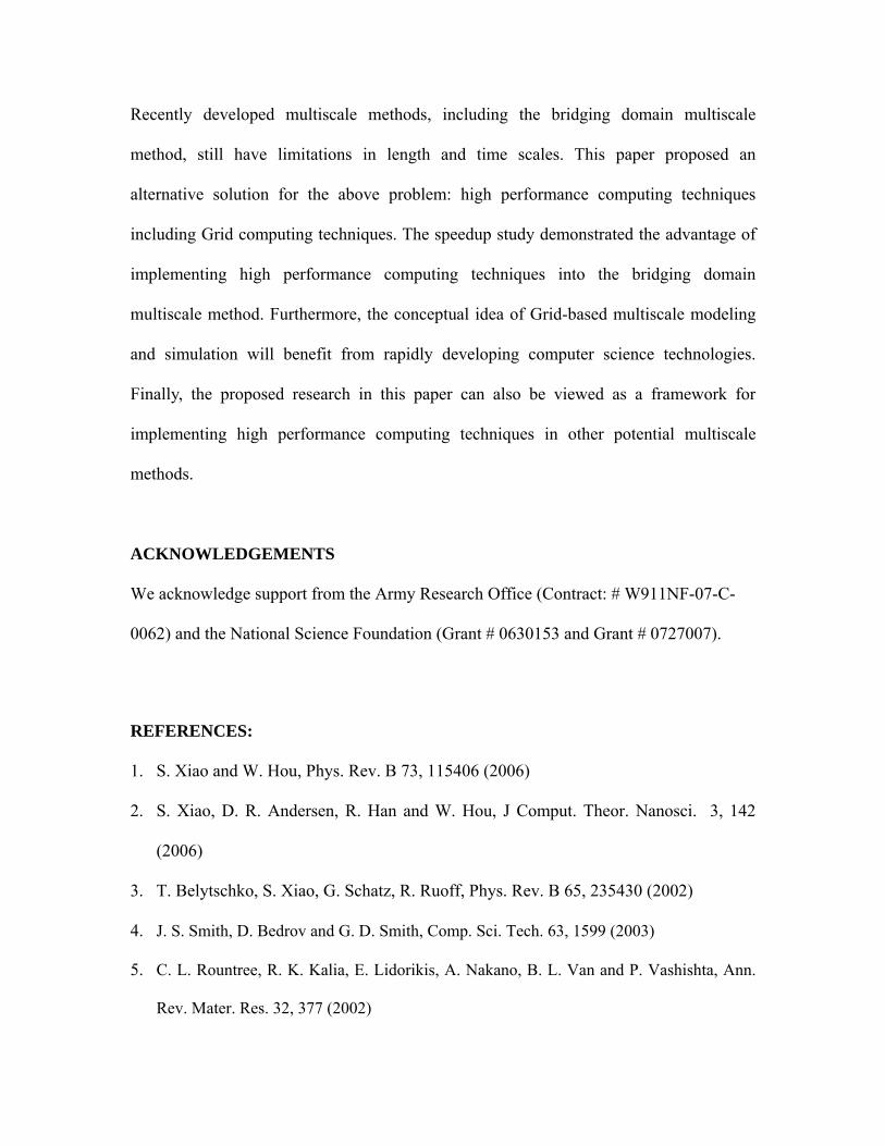
2. Bridging domain coupling method

The Bridging Domain Coupling Method (BDCM) was proposed by Xiao and

Belytschko15,16. Here, we first provide a brief summary of this methodology, detailed in a

one-dimensional molecule chain that includes a molecular dynamics domain, a finite

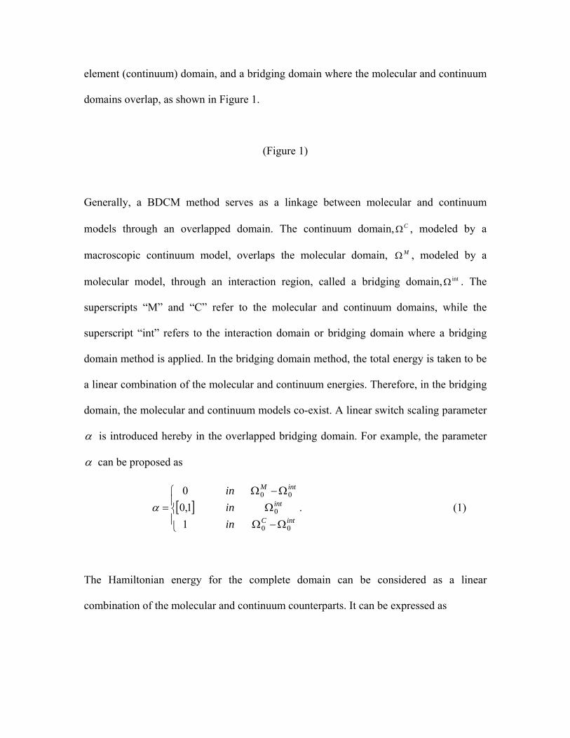
element (continuum) domain, and a bridging domain where the molecular and continuum

domains overlap, as shown in Figure 1.

(Figure 1)

Generally, a BDCM method serves as a linkage between molecular and continuum

models through an overlapped domain. The continuum domain, CΩ , modeled by a

macroscopic continuum model, overlaps the molecular domain, MΩ , modeled by a

molecular model, through an interaction region, called a bridging domain, intΩ . The

superscripts “M” and “C” refer to the molecular and continuum domains, while the

superscript “int” refers to the interaction domain or bridging domain where a bridging

domain method is applied. In the bridging domain method, the total energy is taken to be

a linear combination of the molecular and continuum energies. Therefore, in the bridging

domain, the molecular and continuum models co-exist. A linear switch scaling parameter

α is introduced hereby in the overlapped bridging domain. For example, the parameter

α can be proposed as

[ ]intC

int

intM

ininin

00

0

00

11,0

0

Ω−ΩΩ

Ω−Ω

⎪⎩

⎪⎨

⎧=α . (1)

The Hamiltonian energy for the complete domain can be considered as a linear

combination of the molecular and continuum counterparts. It can be expressed as

( ) ( )

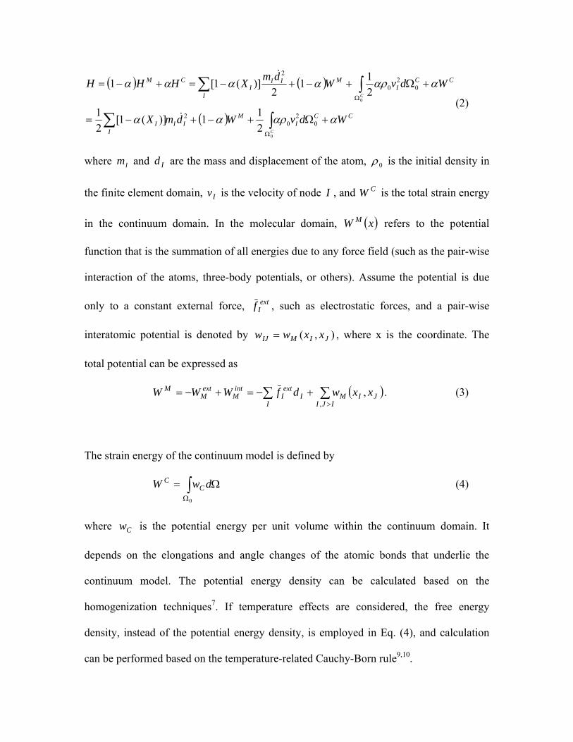
( ) CCI

MII

II

CCI

MII

II

CM

WdvWdmX

WdvWdmXHHH

C

C

ααραα

ααραααα

+Ω+−+−=

+Ω+−+−=+−=

∫∑

∫∑

Ω

Ω

0

0

02

02

02

0

2

211)](1[

21

211

2)](1[1

&

&

(2)

where Im and Id are the mass and displacement of the atom, 0ρ is the initial density in

the finite element domain, Iv is the velocity of node I , and CW is the total strain energy

in the continuum domain. In the molecular domain, ( )xW M refers to the potential

function that is the summation of all energies due to any force field (such as the pair-wise

interaction of the atoms, three-body potentials, or others). Assume the potential is due

only to a constant external force, extIf , such as electrostatic forces, and a pair-wise

interatomic potential is denoted by ),( JIMIJ xxww = , where x is the coordinate. The

total potential can be expressed as

( )∑∑>

+−=+−=IJI

JIMI

Iext

Iint

Mext

MM xxwdfWWW

,, . (3)

The strain energy of the continuum model is defined by

∫Ω

Ω=0

dwW CC (4)

where Cw is the potential energy per unit volume within the continuum domain. It

depends on the elongations and angle changes of the atomic bonds that underlie the

continuum model. The potential energy density can be calculated based on the

homogenization techniques7. If temperature effects are considered, the free energy

density, instead of the potential energy density, is employed in Eq. (4), and calculation

can be performed based on the temperature-related Cauchy-Born rule9,10.

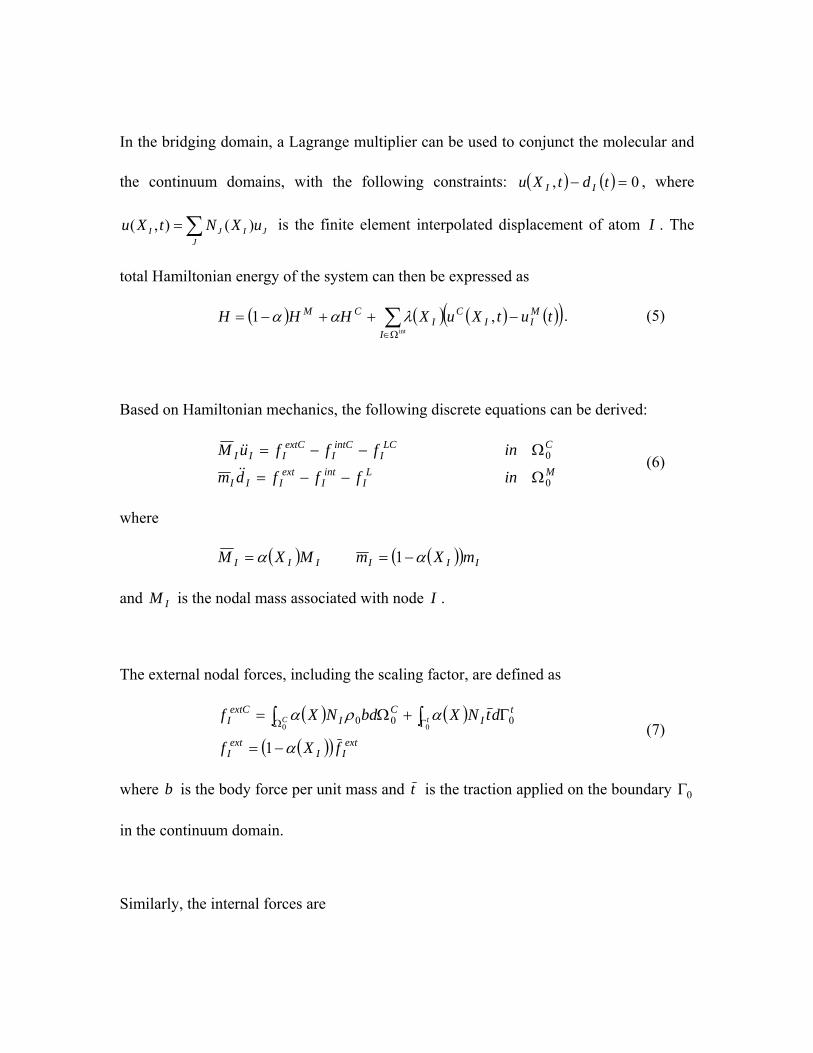
In the bridging domain, a Lagrange multiplier can be used to conjunct the molecular and

the continuum domains, with the following constraints: ( ) ( ) 0, =− tdtXu II , where

∑=J

JIJI uXNtXu )(),( is the finite element interpolated displacement of atom I . The

total Hamiltonian energy of the system can then be expressed as

( ) ( ) ( ) ( )( )∑Ω∈

−++−=int

,1I

MII

CI

CM tutXuXHHH λαα . (5)

Based on Hamiltonian mechanics, the following discrete equations can be derived:

L

Iint

Iext

III

LCI

intCI

extCIII

fffdm

fffuM

−−=

−−=&&

&&

M

C

in

in

0

0

Ω

Ω (6)

where

( ) ( )( ) IIIIII mXmMXM αα −== 1

and IM is the nodal mass associated with node I .

The external nodal forces, including the scaling factor, are defined as

( ) ( )

( )( ) extII

extI

tI

CI

extCI

fXf

dtNXbdNXf tC

α

αρα

−=

Γ+Ω= ∫∫ ΓΩ

100

000 (7)

where b is the body force per unit mass and t is the traction applied on the boundary 0Γ

in the continuum domain.

Similarly, the internal forces are

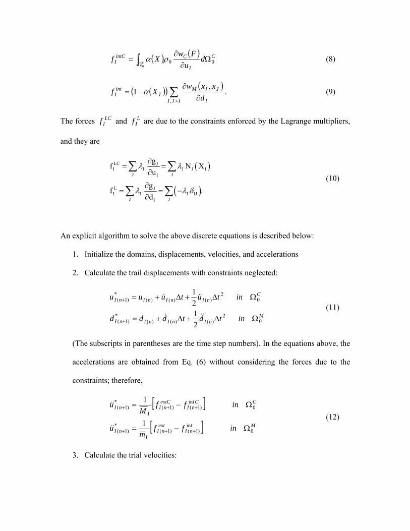
( ) ( )∫Ω Ω

∂∂

= C

C

I

CintCI d

uFw

Xf0

00ρα (8)

( )( ) ( )∑> ∂∂

−=IJI I

JIMI

intI d

xxwXf

,

,1 α . (9)

The forces LCIf and L

If are due to the constraints enforced by the Lagrange multipliers,

and they are

( )

( )

LC JI J J J I

J JI

L JI J J IJ

J JI

gf N Xu

gf .d

λ λ

λ λ δ

∂= =

∂

∂= = −

∂

∑ ∑

∑ ∑ (10)

An explicit algorithm to solve the above discrete equations is described below:

1. Initialize the domains, displacements, velocities, and accelerations

2. Calculate the trail displacements with constraints neglected:

MnInInInI

CnInInInI

intdtddd

intutuuu

02

)()()(*

)1(

02

)()()(*

)1(

2121

ΩΔ+Δ+=

ΩΔ+Δ+=

+

+

&&&

&&&

(11)

(The subscripts in parentheses are the time step numbers). In the equations above, the

accelerations are obtained from Eq. (6) without considering the forces due to the

constraints; therefore,

[ ]

[ ] MnI

extnI

InI

CCnI

extCnI

InI

inffm

u

inffM

u

0int

)1()1(*

)1(

0int

)1()1(*

)1(

1

1

Ω−=

Ω−=

+++

+++

&&

&&

(12)

3. Calculate the trial velocities:

[ ][ ] M

nInInInI

CnInInInI

intdddd

intuuuu

0)1()()(*

)1(

0)1()()(*

)1(

2121

ΩΔ++=

ΩΔ++=

++

++

&&&&&&

&&&&&&

(13)

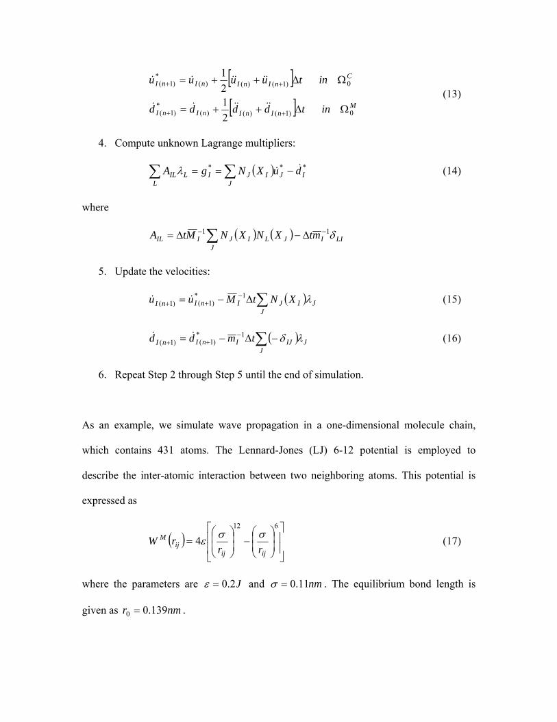
4. Compute unknown Lagrange multipliers:

( ) ***I

JJIJI

LLIL duXNgA && −== ∑∑ λ (14)

where

( ) ( )∑ −− Δ−Δ=J

LIIJLIJIIL mtXNXNMtA δ11

5. Update the velocities:

( )∑Δ−= −++

JJIJInInI XNtMuu λ1*

)1()1( && (15)

( ) JJ

IJInInI tmdd λδ∑ −Δ−= −++

1*)1()1(

&& (16)

6. Repeat Step 2 through Step 5 until the end of simulation.

As an example, we simulate wave propagation in a one-dimensional molecule chain,

which contains 431 atoms. The Lennard-Jones (LJ) 6-12 potential is employed to

describe the inter-atomic interaction between two neighboring atoms. This potential is

expressed as

( )⎥⎥

⎦

⎤

⎢⎢

⎣

⎡

⎟⎟⎠

⎞⎜⎜⎝

⎛−⎟

⎟⎠

⎞⎜⎜⎝

⎛=

612

4ijij

ijM

rrrW σσε (17)

where the parameters are J2.0=ε and nm11.0=σ . The equilibrium bond length is

given as nmr 139.00 = .

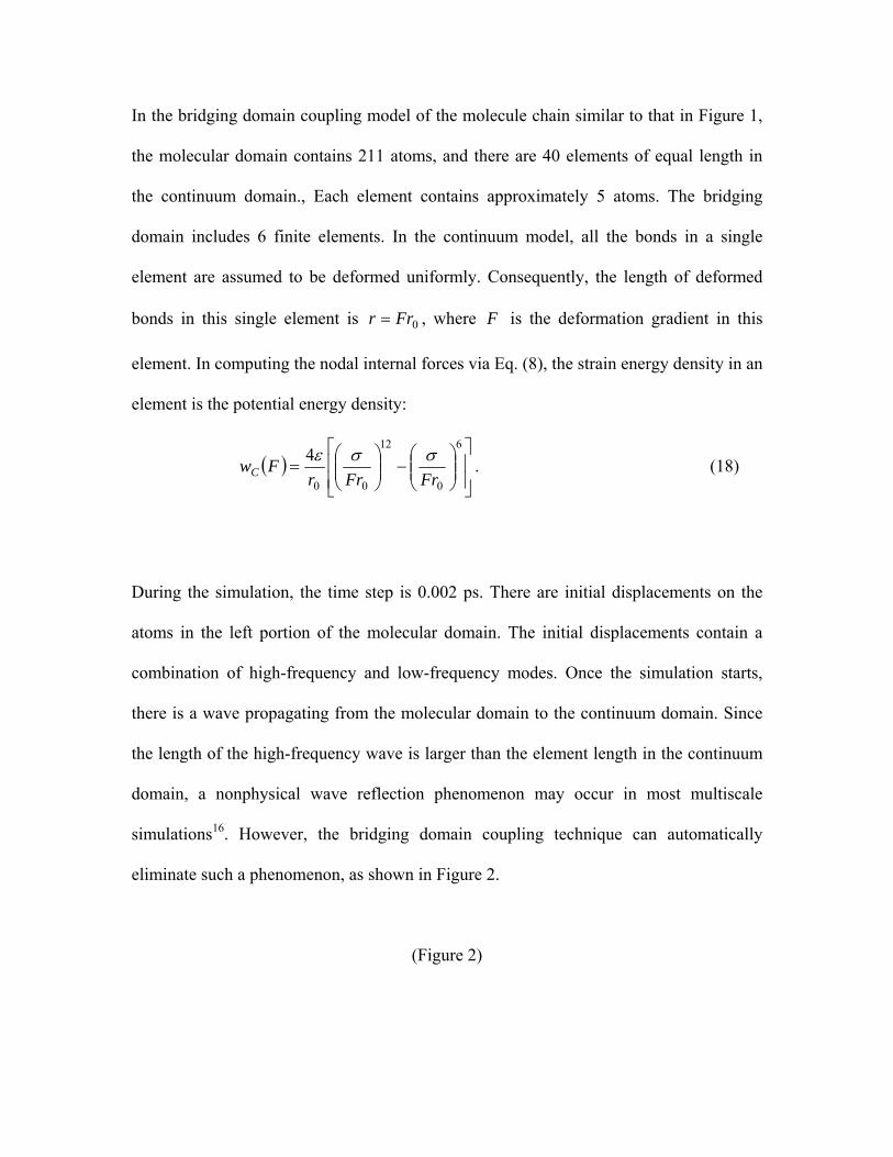
In the bridging domain coupling model of the molecule chain similar to that in Figure 1,

the molecular domain contains 211 atoms, and there are 40 elements of equal length in

the continuum domain., Each element contains approximately 5 atoms. The bridging

domain includes 6 finite elements. In the continuum model, all the bonds in a single

element are assumed to be deformed uniformly. Consequently, the length of deformed

bonds in this single element is 0Frr = , where F is the deformation gradient in this

element. In computing the nodal internal forces via Eq. (8), the strain energy density in an

element is the potential energy density:

( )⎥⎥⎦

⎤

⎢⎢⎣

⎡⎟⎟⎠

⎞⎜⎜⎝

⎛−⎟⎟

⎠

⎞⎜⎜⎝

⎛=

6

0

12

00

4FrFrr

FwCσσε . (18)

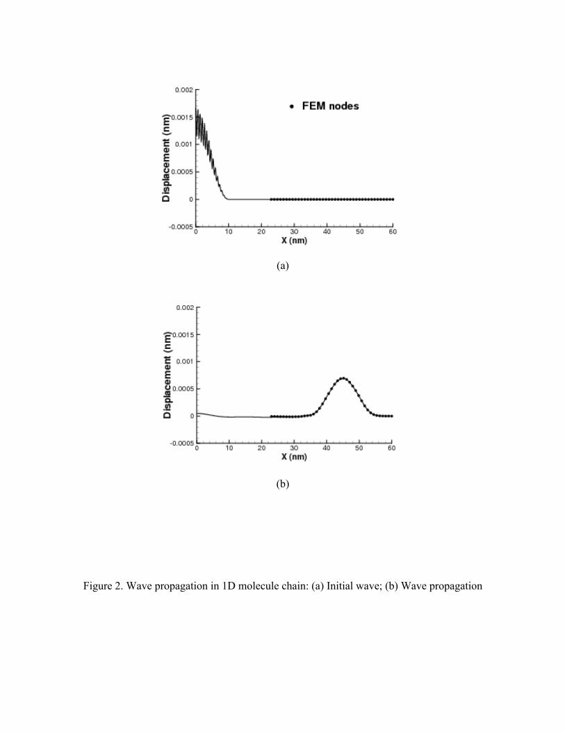
During the simulation, the time step is 0.002 ps. There are initial displacements on the

atoms in the left portion of the molecular domain. The initial displacements contain a

combination of high-frequency and low-frequency modes. Once the simulation starts,

there is a wave propagating from the molecular domain to the continuum domain. Since

the length of the high-frequency wave is larger than the element length in the continuum

domain, a nonphysical wave reflection phenomenon may occur in most multiscale

simulations16. However, the bridging domain coupling technique can automatically

eliminate such a phenomenon, as shown in Figure 2.

(Figure 2)

3. Bridging domain multiscale method with parallel computing

3.1 Bridging domain multiscale method

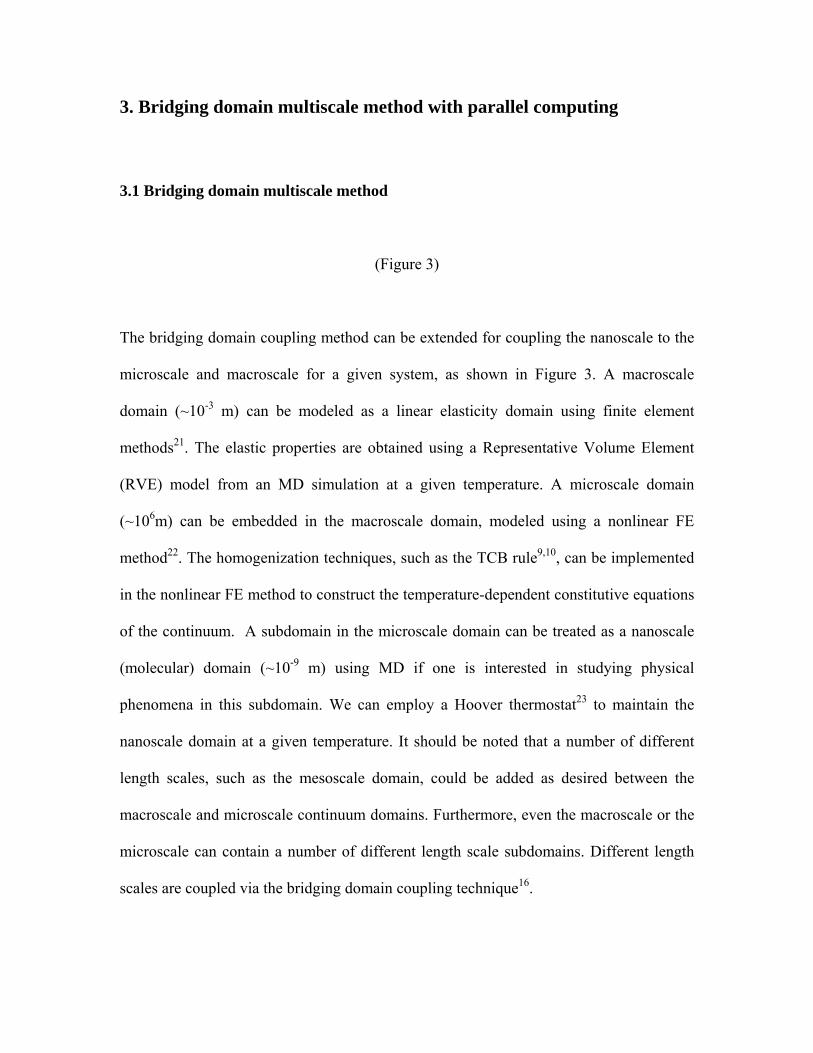
(Figure 3)

The bridging domain coupling method can be extended for coupling the nanoscale to the

microscale and macroscale for a given system, as shown in Figure 3. A macroscale

domain (~10-3 m) can be modeled as a linear elasticity domain using finite element

methods21. The elastic properties are obtained using a Representative Volume Element

(RVE) model from an MD simulation at a given temperature. A microscale domain

(~106m) can be embedded in the macroscale domain, modeled using a nonlinear FE

method22. The homogenization techniques, such as the TCB rule9,10, can be implemented

in the nonlinear FE method to construct the temperature-dependent constitutive equations

of the continuum. A subdomain in the microscale domain can be treated as a nanoscale

(molecular) domain (~10-9 m) using MD if one is interested in studying physical

phenomena in this subdomain. We can employ a Hoover thermostat23 to maintain the

nanoscale domain at a given temperature. It should be noted that a number of different

length scales, such as the mesoscale domain, could be added as desired between the

macroscale and microscale continuum domains. Furthermore, even the macroscale or the

microscale can contain a number of different length scale subdomains. Different length

scales are coupled via the bridging domain coupling technique16.

Most concurrent multiscale methods employ multiple length scales but only a single time

step. In coupling finite element methods and molecular dynamics, if the finite element

mesh is graded down to the atomic spacing at the interface of the continuum and

molecular domains11, the time step must be restricted to the order of one femtosecond

(10-15 s), due to the stability requirement in the molecular model. Consequently,

significant computation time is wasted for large length scales in which large time steps

can be used. In the bridging domain multiscale method, coupling different scales without

such grading down of mesh sizes will be achieved by a straightforward implementation

of different time steps via a multiple-time-step algorithm.

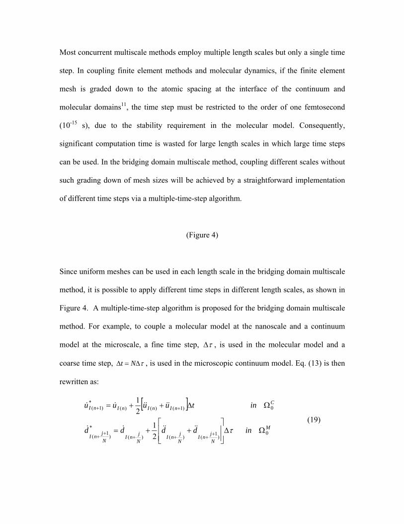
(Figure 4)

Since uniform meshes can be used in each length scale in the bridging domain multiscale

method, it is possible to apply different time steps in different length scales, as shown in

Figure 4. A multiple-time-step algorithm is proposed for the bridging domain multiscale

method. For example, to couple a molecular model at the nanoscale and a continuum

model at the microscale, a fine time step, τΔ , is used in the molecular model and a

coarse time step, τΔ=Δ Nt , is used in the microscopic continuum model. Eq. (13) is then

rewritten as:

[ ]M

NjnI

NjnI

NjnI

NjnI

CnInInInI

indddd

intuuuu

0)1()()(

*

)1(

0)1()()(*

)1(

21

21

ΩΔ⎥⎥⎦

⎤

⎢⎢⎣

⎡++=

ΩΔ++=

++++

++

++

τ&&&&&&

&&&&&&

(19)

The bridging domain then connects a fine length/time scale and a coarse length/time

scale. Compatibility of different length scales will be enforced by means of a constraint

imposed via the Lagrange multiplier method, i.e., Eq. (14), at each coarse time step, tΔ ,

as shown in Figure 4. Consequently, the equations of motion will be solved

independently in different length scales with different time steps. At each coarse time

step, velocities of nodes/atoms in the bridging domain will be corrected via the bridging

domain coupling technique.

3.2 Domain Decomposition

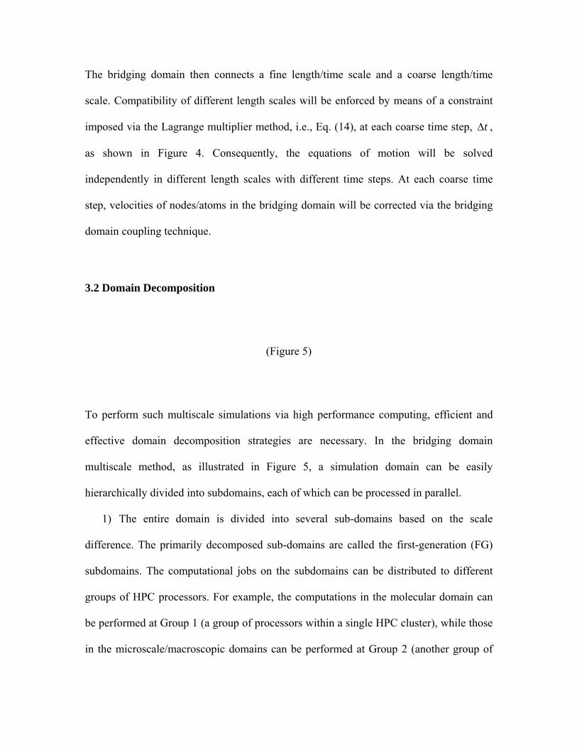
(Figure 5)

To perform such multiscale simulations via high performance computing, efficient and

effective domain decomposition strategies are necessary. In the bridging domain

multiscale method, as illustrated in Figure 5, a simulation domain can be easily

hierarchically divided into subdomains, each of which can be processed in parallel.

1) The entire domain is divided into several sub-domains based on the scale

difference. The primarily decomposed sub-domains are called the first-generation (FG)

subdomains. The computational jobs on the subdomains can be distributed to different

groups of HPC processors. For example, the computations in the molecular domain can

be performed at Group 1 (a group of processors within a single HPC cluster), while those

in the microscale/macroscopic domains can be performed at Group 2 (another group of

processors within a single HPC cluster). The first-generation subdomain decomposition is

parallel computing task decomposition. Each FG subdomain is further divided into a

number of second-generation (SG) subdomains. Each SG subdomain is assigned to a

single processor. In other words, as the secondary effort, the data within the subdomain

are decomposed and transferred to each processor within a specified group for intensive

computation. Obviously, it is a data-decomposition. This way, the task and data

decomposition are combined.

2) A bridging subdomain is a special subdomain. It is shared by two SG subdomains,

each of which belongs to two different length scales. Although one SG subdomain can

overlap more than one other SG subdomain, the bridging subdomains do not overlap each

other.

3) Inter-domain communications between two SG subdomains take place in each FG

subdomain separately. Such inter-domain communications occur prior to solution of the

equations of motion so that the motion of atoms or nodes at the SG subdomain

boundaries is consistent.

4) The procedure for solving equations of motion in each FG subdomain is

independent.

5) Once the equations of motion are solved at each time step (or coarse time step in

the event that a multiple-time-step algorithm is used), the bridging domain

communications take place between two processors. It should be noted that those two

processors belong to two different groups of processors, shown in Figure 4. The bridging

coupling techniques are applied to correct the trial velocities of nodes or atoms in each

bridging subdomain independently.

3.3 Inter-domain and bridging domain communications

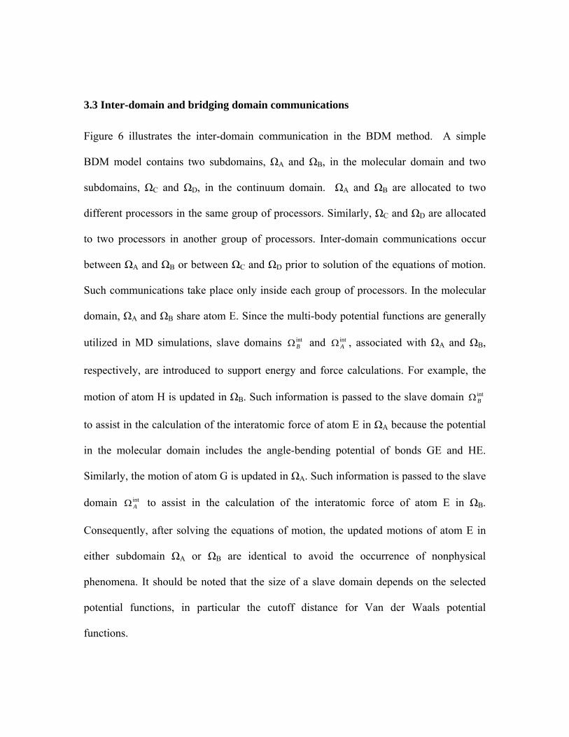
Figure 6 illustrates the inter-domain communication in the BDM method. A simple

BDM model contains two subdomains, ΩA and ΩB, in the molecular domain and two

subdomains, ΩC and ΩD, in the continuum domain. ΩA and ΩB are allocated to two

different processors in the same group of processors. Similarly, ΩC and ΩD are allocated

to two processors in another group of processors. Inter-domain communications occur

between ΩA and ΩB or between ΩC and ΩD prior to solution of the equations of motion.

Such communications take place only inside each group of processors. In the molecular

domain, ΩA and ΩB share atom E. Since the multi-body potential functions are generally

utilized in MD simulations, slave domains intBΩ and int

AΩ , associated with ΩA and ΩB,

respectively, are introduced to support energy and force calculations. For example, the

motion of atom H is updated in ΩB. Such information is passed to the slave domain intBΩ

to assist in the calculation of the interatomic force of atom E in ΩA because the potential

in the molecular domain includes the angle-bending potential of bonds GE and HE.

Similarly, the motion of atom G is updated in ΩA. Such information is passed to the slave

domain intAΩ to assist in the calculation of the interatomic force of atom E in ΩB.

Consequently, after solving the equations of motion, the updated motions of atom E in

either subdomain ΩA or ΩB are identical to avoid the occurrence of nonphysical

phenomena. It should be noted that the size of a slave domain depends on the selected

potential functions, in particular the cutoff distance for Van der Waals potential

functions.

(Figure 6)

The inter-domain communication in the continuum domain has a different strategy from

the one in the molecular domain. The continuum subdomains ΩC and ΩD share the

boundary node F, as shown in Figure 6. FC and FD are used to represent the same node F,

but in different subdomains. Unlike inter-domain communication between neighboring

molecular subdomains, inter-domain communication between neighboring continuum

subdomains does not require slave domains, instead acting to aid the exchange of

calculated internal forces of boundary nodes. For instance, the internal force of node FC,

calculated in subdomain ΩC, is passed to subdomain ΩD and is set as the negatively

external force of node FD. A similar procedure is performed to pass the internal force of

node FD, calculated in subdomain ΩD, to subdomain ΩC as the negatively external force

of node FC. Therefore, the motions of node F, updated by solving the equations of

motion, Eq. (6), in both subdomains ΩC and ΩD, are identical.

(Figure 7)

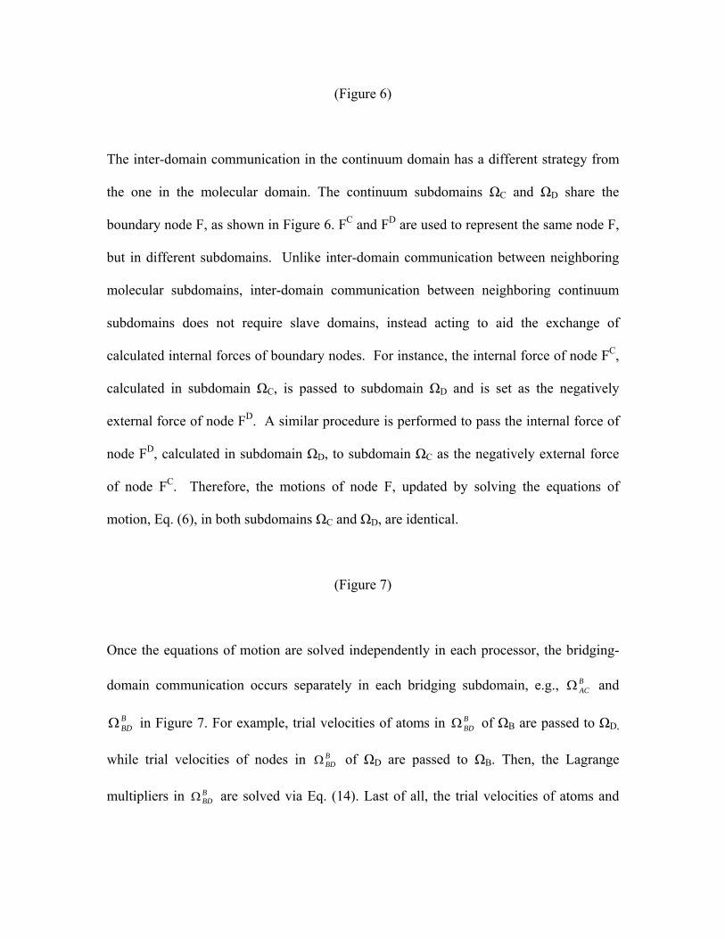
Once the equations of motion are solved independently in each processor, the bridging-

domain communication occurs separately in each bridging subdomain, e.g., BACΩ and

BBDΩ in Figure 7. For example, trial velocities of atoms in B

BDΩ of ΩB are passed to ΩD,

while trial velocities of nodes in BBDΩ of ΩD are passed to ΩB. Then, the Lagrange

multipliers in BBDΩ are solved via Eq. (14). Last of all, the trial velocities of atoms and

nodes in the bridging domain BBDΩ will be corrected in ΩB and ΩD, independently

through Eqs. (15) and (16).

Upon the above domain decomposition and data communication, the parallel computing

processing can be implemented in the workflow illustrated in Figure 8.

(Figure 8)

3.4 Complexity and performance evaluations

An important focus of the proposed method is the definition of a suitable computational

intensity metric for sub-domains:

M ( d ) = f ( D ( d ), O, P ) (20)

where M is a function of the domain size D, i.e., the number of nodes or atoms having

sub-domain d, the computing time complexity O of a particular component of a

multiscale method, and parameters P that characterize the computing capacity of each

specific HPC resource. M will be used to determine the size of sub-domains in domain

decomposition. M is also an important parameter that can be used to guide decisions

about when and where these sub-domains should be scheduled.

The computing time complexity of a continuum domain is O(n2) while the complexity for

a molecular domain is O(m2), where m represents the number of atoms and n the number

of finite element nodes. Although the complexity representation is the same for these

two domains, m is often significantly larger than n. O(m2) is approximately within the

range O(n3) to O(n4), because m is approximately equivalent to n3/2~2. The domain

decomposition approach will address this complexity difference to produce sub-domains

adaptively, the representations of which include the complexity information for tasking

scheduling purposes. This approach will help detach the domain decomposition technique

from the task-scheduling advisor, as described in the following. Further research will be

conducted for multiple time steps as used in different length scales.

In order to investigate the feasibility, reliability, and application of the proposed method,

several high performance computing benchmark studies should be conducted. The studies

include (1) parallel performance speedup and efficiency to evaluate the behavior of high-

performance computing, (2) detailed data communication (blocking, non-blocking,

gather/scatter, one-site-communication effect using MPI2 features, parallel I/O, network

impacts and network latency, load balance, etc.) among a group of processors and

computational nodes to understand and reduce the communication loss, and

(3) experiments of different HPC platforms and an analytical model of HPC scalability.

3.5 One-dimensional examples

To demonstrate the preliminary feasibility of the bridging domain multiscale method with

high performance computing techniques, an experimental model has been developed.

Similar to the previous example, the experiment is designed to observe the propagation of

an imposed wave in a molecule chain passing from the molecular domain to the

continuum domain. In this example, the bridging domain multiscale model contains

10,000 atoms and 10,000 finite elements. Each finite element contains 9 atoms.

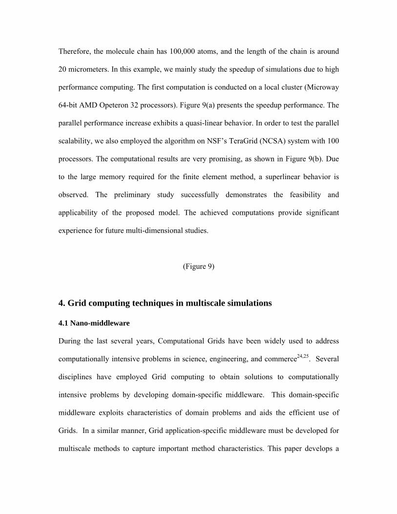
Therefore, the molecule chain has 100,000 atoms, and the length of the chain is around

20 micrometers. In this example, we mainly study the speedup of simulations due to high

performance computing. The first computation is conducted on a local cluster (Microway

64-bit AMD Opeteron 32 processors). Figure 9(a) presents the speedup performance. The

parallel performance increase exhibits a quasi-linear behavior. In order to test the parallel

scalability, we also employed the algorithm on NSF’s TeraGrid (NCSA) system with 100

processors. The computational results are very promising, as shown in Figure 9(b). Due

to the large memory required for the finite element method, a superlinear behavior is

observed. The preliminary study successfully demonstrates the feasibility and

applicability of the proposed model. The achieved computations provide significant

experience for future multi-dimensional studies.

(Figure 9)

4. Grid computing techniques in multiscale simulations

4.1 Nano-middleware

During the last several years, Computational Grids have been widely used to address

computationally intensive problems in science, engineering, and commerce24,25. Several

disciplines have employed Grid computing to obtain solutions to computationally

intensive problems by developing domain-specific middleware. This domain-specific

middleware exploits characteristics of domain problems and aids the efficient use of

Grids. In a similar manner, Grid application-specific middleware must be developed for

multiscale methods to capture important method characteristics. This paper develops a

conceptual framework for multiscale methods that supports the location, allocation, and

utilization of Grid resources to effectively and efficiently apply multiscale methods for

nanotechnology applications. This middleware is referred to as nano-middleware in this

paper.

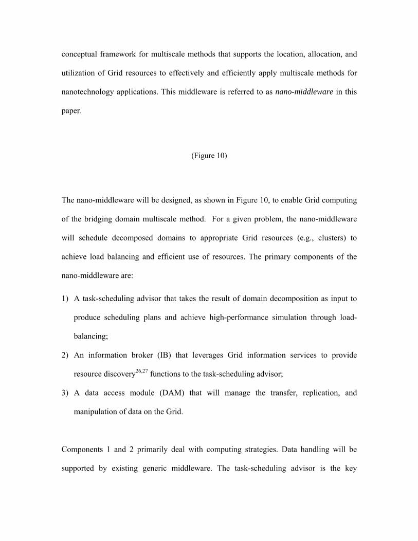
(Figure 10)

The nano-middleware will be designed, as shown in Figure 10, to enable Grid computing

of the bridging domain multiscale method. For a given problem, the nano-middleware

will schedule decomposed domains to appropriate Grid resources (e.g., clusters) to

achieve load balancing and efficient use of resources. The primary components of the

nano-middleware are:

1) A task-scheduling advisor that takes the result of domain decomposition as input to

produce scheduling plans and achieve high-performance simulation through load-

balancing;

2) An information broker (IB) that leverages Grid information services to provide

resource discovery26,27 functions to the task-scheduling advisor;

3) A data access module (DAM) that will manage the transfer, replication, and

manipulation of data on the Grid.

Components 1 and 2 primarily deal with computing strategies. Data handling will be

supported by existing generic middleware. The task-scheduling advisor is the key

element of nano-middleware for its impact on performance gains. It should be noted that

the concept of proposed nano-middleware can be applied to other multiscale methods.

4.2 Task scheduling advisor

Task scheduling is used to schedule subdomains to an appropriate set of Grid resources to

achieve optimal performance—tasks are allocated in a way that balances computation

across the selection of available resources. In the nano-middleware task-scheduling

advisor, subdomains from the computational domain decomposition process are

converted to tasks that are then placed in Grid resource queues in a specific order. In

practice, queues will be managed by local resource schedulers, such as Portable Batch

Systems (PBS) and Condor. The task-scheduling advisor is designed to achieve optimal

performance by balancing tasks across available resources28. The advisor generates a

scheduling plan that determines the correspondence between tasks and the available Grid

resources to which they are submitted.

There are two general approaches to task scheduling: static and dynamic. When a static

scheduling strategy is employed, the scheduling plan does not change until all tasks are

completed29. In contrast, dynamic scheduling permits a plan to be altered while the set of

tasks is being executed30. Using dynamic task scheduling for the BDM method is

difficult to accomplish for two specific reasons31. First, the computation required to

implement dynamic scheduling is much greater than for static scheduling; dynamic

scheduling introduces additional overhead penalties created by network latency and the

execution of the code that monitors the task status. Also, tasks are swapped between

resources according to a dynamic performance evaluation. Second, fine granularity in

individual subdomains, produced based on the BDM method, is desirable in order to

achieve high levels of parallelism. Results for these subdomains can be inexpensive to

compute even if scheduled to a Grid resource having a small capacity. Therefore, the

time overhead that results from implementing dynamic scheduling on a task level may

exceed the time required to compute results for an individual subdomain.

Consequently, static scheduling strategies are developed to assign tasks based on

computational intensity information for each subdomain, as well as the variability in the

computing capacity of each Grid resource. Two principles are used to guide the

development of static scheduling algorithms: (1) Grid resources with greater computing

capacity are used before those with less capacity; and (2) tasks that are more (less)

computationally intensive are assigned to Grid resources with more (less) computing

capacity32.

5. Conclusions

Multiscale modeling and simulation has been at the forefront of nanotechnology research

due to its ability to simulate larger systems than is possible with molecular dynamics. In

this paper, we first introduced the bridging domain coupling method, which can

efficiently couple molecular dynamics and the finite element method. A more powerful

multiscale method can be extended to bridge a number of length and time scales via the

bridging domain coupling technique.

Recently developed multiscale methods, including the bridging domain multiscale

method, still have limitations in length and time scales. This paper proposed an

alternative solution for the above problem: high performance computing techniques

including Grid computing techniques. The speedup study demonstrated the advantage of

implementing high performance computing techniques into the bridging domain

multiscale method. Furthermore, the conceptual idea of Grid-based multiscale modeling

and simulation will benefit from rapidly developing computer science technologies.

Finally, the proposed research in this paper can also be viewed as a framework for

implementing high performance computing techniques in other potential multiscale

methods.

ACKNOWLEDGEMENTS

We acknowledge support from the Army Research Office (Contract: # W911NF-07-C-

0062) and the National Science Foundation (Grant # 0630153 and Grant # 0727007).

REFERENCES:

1. S. Xiao and W. Hou, Phys. Rev. B 73, 115406 (2006)

2. S. Xiao, D. R. Andersen, R. Han and W. Hou, J Comput. Theor. Nanosci. 3, 142

(2006)

3. T. Belytschko, S. Xiao, G. Schatz, R. Ruoff, Phys. Rev. B 65, 235430 (2002)

4. J. S. Smith, D. Bedrov and G. D. Smith, Comp. Sci. Tech. 63, 1599 (2003)

5. C. L. Rountree, R. K. Kalia, E. Lidorikis, A. Nakano, B. L. Van and P. Vashishta, Ann.

Rev. Mater. Res. 32, 377 (2002)

6. S. Xiao and W. Hou, Phys. Rev. B 75, 125414 (2007)

7. E. B. Tadmor, M. Ortiz and R. Phillips, Phil. Mag. A 73, 1529 (1996)

8. S. Q. Chen, W. N. E and C. W. Shu, Mult. Model. Simul. 3, 871 (2005)

9. S. Xiao and W. Yang, Int. J. Numer. Meth. Engrg. 69, 2099 (2007)

10. S. Xiao and W. Yang, Comp. Mater. Sci. 37, 374 (2006)

11. F. Abraham, J. Broughton, N. Bernstein and E. Kaxiras, Europhy. Lett. 44, 783 (1998)

12. J. Broughton, F. Abraham, N. Bernstein and E. Kaxiras, Phys. Rev. B 60, 2391 (1999)

13. N. Choly, G. Lu, W. E and E. Kaxiras, Phys. Rev. B 71, 094101 (2005)

14. G. J. Wagner and W. K. Liu, J. Comp. Phys. 190, 249 (2003)

15. T. Belytschko and S. P. Xiao, Int. J. Multi. Comp. Engrg. 1, 115 (2003)

16. S. P. Xiao and T. Belytschko, Comp. Meth. Appl. Mech. Engrg. 193, 1645 (2004)

17. Y. G. Yanovsky, Int. J. Multi. Comp. Engrg. 3, 199 (2005)

18. J. Ma, H. Lu, B. Wang, R. Hornung, A. Wissink, and R. Komanduri, Comp. Model.

Engrg. Sci. 14, 101 (2006)

19. I. Foster and C. Kesselman, The Grid: Blue Print for a New Computing Infrastructure.

Morgan Kaufmann Publishers, Inc. San Francisco, CA, 1999

20. I. Foster, C. Kesselman and S. Tuecke, Int. J. Supercomp. Appl. 15, (2001)

21. T. J. R. Hughes, The Finite Element Method: Linear Static and Dynamic Analysis,

Prentice-Hall, Dover, 1987.

22. T. Belytschko, W. K. Liu and B. Moran, Nonlinear Finite Elements for Continua and

Structures, Wiley, New York, 2000

23. W. G. Hoover, Phys. Rev. A 31, 1695 (1985)

24. I. Foster, Phys. Today 55, 42 (2002)

25. F. Berman, G. Fox and T. Hey, “The Grid, past, present, future,” In Grid Computing,

Making the Global Infrastructure a Reality, edited by R. Berman, G. Fox, and T. Hey

John Wiley & Sons, West Sussex, England, 2003

26. S. Wang, A. Padmanabhan, Y. Liu, R. Briggs, J. Ni, T. He, B. M. Knosp, Y. Onel, Lec.

Note. Comp. Sci. 3032, 536 (2003)

27. Padmanabhan, A., Wang, S., Ghosh, S., and Briggs, R. Proceedings of the Grid 2005

Workshop, Seattle, WA, November 13-14, 2005, IEEE press, pp. 312-317.

28. J. Henrichs, Proceedings of International Conference on Supercomputing 1998, 165

(1998)

29. T. D. Braun, H. J. Siegel, N. Beck, L. L. Boloni, M. Maheswaran, A. I. Reuther, J. P.

Robertson, M. D. Theys, B. Yao, D. Hensgen and R. F. Freund, J. Para. Distrib. Comp.

61, 810 (2001)

30. O. Beaumont, A. Legrand and Y. Robert, Para. Comp. 29, 1121 (2003)

31. H. J. Siegel and S. Ali, Euromicro J. Sys. Arch. 46, 627 (2000)

32. S. Wang and M. P. Armstrong, Para. Comp. 29, 1481 (2003)

Figure 1. Bridging domain coupling model of a molecule chain

(a)

(b)

Figure 2. Wave propagation in 1D molecule chain: (a) Initial wave; (b) Wave propagation

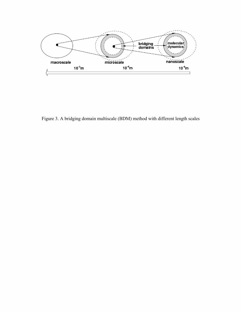
Figure 3. A bridging domain multiscale (BDM) method with different length scales

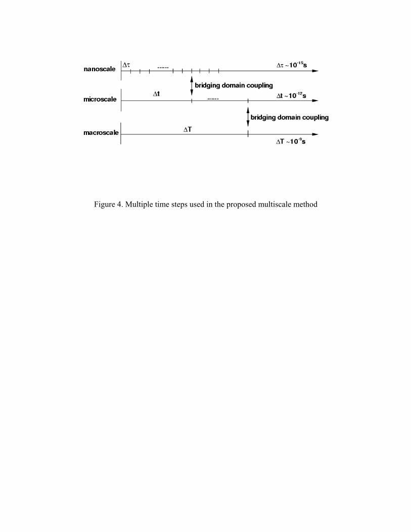
Figure 4. Multiple time steps used in the proposed multiscale method

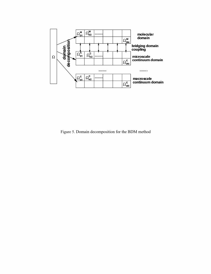
Figure 5. Domain decomposition for the BDM method

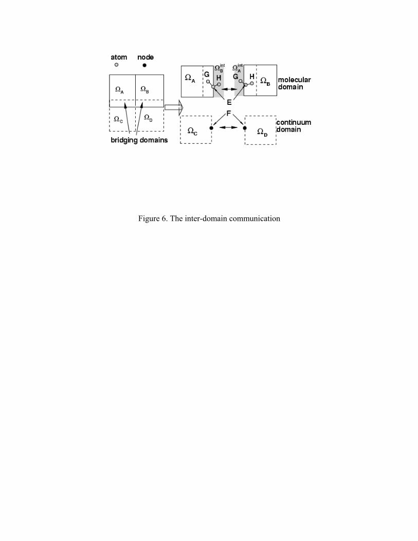
Figure 6. The inter-domain communication

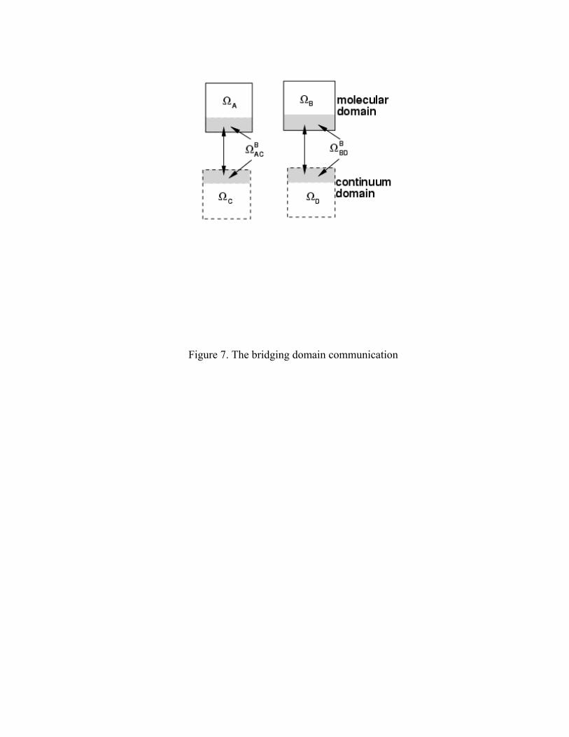
Figure 7. The bridging domain communication

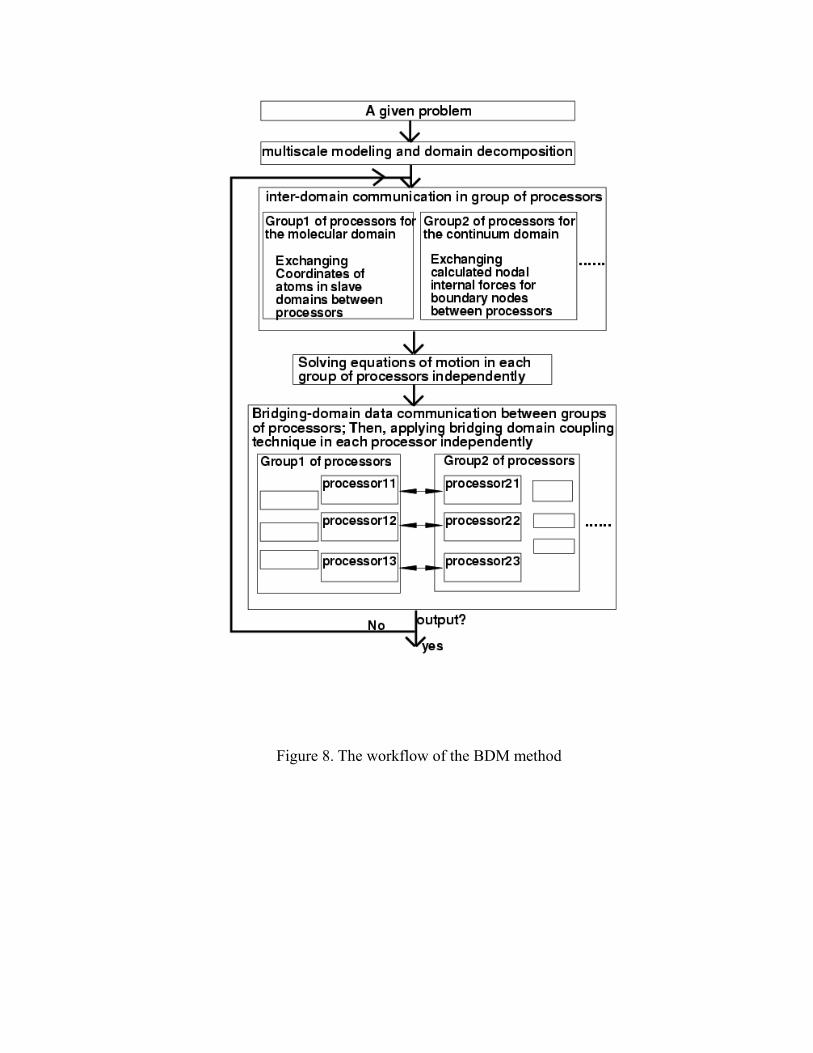
Figure 8. The workflow of the BDM method

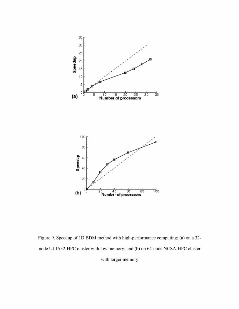
Figure 9. Speedup of 1D BDM method with high-performance computing; (a) on a 32-

node UI-IA32-HPC cluster with low memory; and (b) on 64-node NCSA-HPC cluster

with larger memory

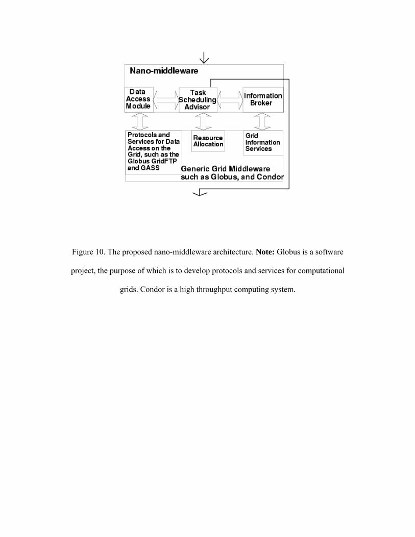
Figure 10. The proposed nano-middleware architecture. Note: Globus is a software

project, the purpose of which is to develop protocols and services for computational

grids. Condor is a high throughput computing system.