A Generative Model for Music Transcription

1

A Generative Model for Music TranscriptionAli Taylan Cemgil,Student Member, IEEE,Bert Kappen,Senior Member, IEEE,and David Barber

Abstract— In this paper we present a graphical model forpolyphonic music transcription. Our model, formulated as aDynamical Bayesian Network, embodies a transparent and com-putationally tractable approach to this acoustic analysis problem.An advantage of our approach is that it places emphasis onexplicitly modelling the sound generation procedure. It providesa clear framework in which both high level (cognitive) priorinformation on music structure can be coupled with low level(acoustic physical) information in a principled manner to performthe analysis. The model is a special case of the, generallyintractable, switching Kalman filter model. Where possible,we derive, exact polynomial time inference procedures, andotherwise efficient approximations. We argue that our generativemodel based approach is computationally feasible for many musicapplications and is readily extensible to more general auditoryscene analysis scenarios.

Index Terms— music transcription, polyphonic pitch tracking,Bayesian signal processing, switching Kalman filters

I. I NTRODUCTION

When humans listen to sound, they are able to associateacoustical signals generated by different mechanisms withindividual symbolic events [1]. The study and computationalmodelling of this human ability forms the focus of computa-tional auditory scene analysis (CASA) and machine listening[2]. Research in this area seeks solutions to a broad rangeof problems such as the cocktail party problem, (for exampleautomatically separating voices of two or more simultaneouslyspeaking persons, see e.g. [3], [4]), identification of envi-ronmental sound objects [5] and musical scene analysis [6].Traditionally, the focus of most research activities has beenin speech applications. Recently, analysis of musical scenesis drawing increasingly more attention, primarily because ofthe need for content based retrieval in very large digitalaudio databases [7] and increasing interest in interactive musicperformance systems [8].

A. Music Transcription

One of the hard problems in musical scene analysis is au-tomatic music transcription, that is, the extraction of a humanreadable and interpretable description from a recording of amusic performance. Ultimately, we wish to infer automaticallya musical notation (such as the traditional western musicnotation) listing the pitch levels of notes and correspondingtime-stamps for a given performance. Such a representationof the surface structure of music would be very useful in

Manuscript received; revised .A. T. Cemgil is with University of Amsterdam, Informatica Instituut, Kruis-

laan 403, 1098 SJ Amsterdam, the Netherlands, B. Kappen is with RadboudUniversity Nijmegen, SNN, Geert Grooteplein 21, 6525 EZ Nijmegen, theNetherlands and D. Barber is with IDIAP, CH-1920 Martigny, Switzerland.

a broad spectrum of applications such as interactive musicperformance systems, music information retrieval (Music-IR)and content description of musical material in large audiodatabases, as well as in the analysis of performances. In itsmost unconstrained form, i.e., when operating on an arbitrarypolyphonic acoustical input possibly containing an unknownnumber of different instruments, automatic music transcriptionremains a great challenge. Our aim in this paper is to considera computational framework to move us closer to a practicalsolution of this problem.

Music transcription has attracted significant research effortin the past – see [6] and [9] for a detailed review of earlyand more recent work, respectively. In speech processing, therelated task of tracking the pitch of a single speaker is afundamental problem and methods proposed in the literatureare well studied[10]. However, most current pitch detectionalgorithms are based largely on heuristics (e.g., picking highenergy peaks of a spectrogram, correlogram, auditory filterbank, etc.) and their formulation usually lacks an explicitobjective function or signal model. It is often difficult totheoretically justify the merits and shortcomings of suchalgorithms, and compare them objectively to alternatives orextend them to more complex scenarios.

Pitch tracking is inherently related to the detection andestimation of sinusoids. The estimation and tracking of singleor multiple sinusoids is a fundamental problem in manybranches of applied sciences, so it is less surprising that thetopic has also been deeply investigated in statistics, (e.g. see[11]). However, ideas from statistics seem to be not widelyapplied in the context of musical sound analysis, with only afew exceptions [12], [13] who present frequentist techniquesfor very detailed analysis of musical sounds with particularfocus on decomposition of periodic and transient components.[14] has presented real-time monophonic pitch tracking ap-plication based on a Laplace approximation to the posteriorparameter distribution of an AR(2) model [15], [11, page19]. Their method outperforms several standard pitch trackingalgorithms for speech, suggesting potential practical benefits ofan approximate Bayesian treatment. For monophonic speech,a Kalman filter based pitch tracker is proposed by [16] thattracks parameters of a harmonic plus noise model (HNM).They propose the use of Laplace approximation around thepredicted mean instead of the extended Kalman filter (EKF).For both methods, however, it is not obvious how to extendthem to polyphony.

Kashino [17] is, to our knowledge, the first author to applygraphical models explicitly to the problem of polyphonicmusic transcription. Sterian [18] described a system thatviewed transcription as a model driven segmentation of atime-frequency image. Walmsley [19] treats transcription andsource separation in a full Bayesian framework. He employs a0000–0000/00$00.00c© 2004 IEEE

2

frame based generalized linear model (a sinusoidal model) andproposes inference by reversible-jump Markov Chain MonteCarlo (MCMC) algorithm. The main advantage of the model isthat it makes no strong assumptions about the signal generationmechanism, and views the number of sources as well as thenumber of harmonics as unknown model parameters. Davy andGodsill [20] address some of the shortcomings of his modeland allow changing amplitudes and frequency deviations.The reported results are encouraging, although the method iscomputationally very expensive.

B. Approach

Musical signals have a very rich temporal structure, bothon a physical (signal) and a cognitive (symbolic) level. Froma statistical modelling point of view, such a hierarchicalstructure induces very long range correlations that are difficultto capture with conventional signal models. Moreover, in manymusic applications, such as transcription or score following,we are usually interested in a symbolic representation (suchas a score) and not so much in the “details” of the actualwaveform. To abstract away from the signal details, we definea set of intermediate variables (a sequence of indicators),somewhat analogous to a “piano-roll” representation. Thisintermediate layer forms the “interface” between a symbolicprocess and the actual signal process. Roughly, the symbolicprocess describes how a piece is composed and performed.We view this process as a prior distribution on the piano-roll. Conditioned on the piano-roll, the signal process describeshow the actual waveform is synthesized.

Most authors view automated music transcription as an “au-dio to piano-roll” conversion and usually consider “piano-rollto score” a separate problem. This view is partially justified,since source separation and transcription from a polyphonicsource is already a challenging task. On the other hand,automated generation of a human readable score includesnontrivial tasks such as tempo tracking, rhythm quantization,meter and key induction [21], [22], [23]. As also noted byother authors (e.g. [17], [24], [25]), we believe that a modelthat integrates this higher level symbolic prior knowledge canguide and potentially improve the inferences, both in termsquality of a solution and computation time.

There are many different natural generative models forpiano-rolls. In [26], we proposed a realistic hierarchical priormodel. In this paper, we consider computationally simplerprior models and focus more on developing efficient inferencetechniques of a piano-roll representation. The organization ofthe paper is as follows: We will first present a generativemodel, inspired by additive synthesis, that describes the signalgeneration procedure. In the sequel, we will formulate twosubproblems related to music transcription: melody identifica-tion and chord identification. We will show that both problemscan be easily formulated as combinatorial optimization prob-lems in the framework of our model, merely by redefining theprior on piano-rolls. Under our model assumptions, melodyidentification can be solved exactly in polynomial time (inthe number of samples). By deterministic pruning, we obtaina practical approximation that works in linear time. Chord

identification suffers from combinatorial explosion. For thiscase, we propose a greedy search algorithm based on iterativeimprovement. Consequently, we combine both algorithms forpolyphonic music transcription. Finally, we demonstrate how(hyper-)parameters of the signal process can be estimated fromreal data.

II. POLYPHONIC MODEL

In a statistical sense, music transcription, (as many otherperceptual tasks such as visual object recognition or robot lo-calization) can be viewed as a latent state estimation problem:given the audio signal, we wish to identify the sequence ofevents (e.g. notes) that gave rise to the observed audio signal.

This problem can be conveniently described in a Bayesianframework: given the audio samples, we wish to infer a piano-roll that represents the onset times (e.g. times at which a‘string’ is ‘plucked’), note durations and the pitch classes ofindividual notes. We assume that we have one microphone, sothat at each timet we have a one dimensional observed quan-tity yt. Multiple microphones (such as required for processingstereo recordings) would be straightforward to include in ourmodel. We denote the temporal sequence of audio samples{y1, y2, . . . , yt, . . . , yT } by the shorthand notationy1:T . Aconstant sampling frequencyFs is assumed.

Our approach considers the quantities we wish to infer asa collection of ‘hidden’ variables, whilst acoustic recordingvaluesy1:T are ‘visible’ (observed). For each observed sampleyt, we wish to associate a higher, unobserved quantity thatlabels the sampleyt appropriately. Let us denote the unob-served quantities byH1:T where eachHt is a vector. Ourhidden variables will contain, in addition to a piano-roll, othervariables required to complete the sound generation procedure.We will elucidate their meaning later. As a general inferenceproblem, the posterior distribution is given by Bayes’ rule

p(H1:T |y1:T ) ∝ p(y1:T |H1:T )p(H1:T ) (1)

The likelihood termp(y1:T |H1:T ) in (1) requires us to specifya generative process that gives rise to the observed audiosamples. The prior termp(H1:T ) reflects our knowledge aboutpiano-rolls and other hidden variables. Our modelling task istherefore to specify both how, knowing the hidden variablestates (essentially the piano-roll), the microphone samples willbe generated, and also to state a prior on likely piano-rolls.Initially, we concentrate on the sound generation process of asingle note.

A. Modelling a single note

Musical instruments tend to create oscillations with modesthat are roughly related by integer ratios, albeit with strongdamping effects and transient attack characteristics [27]. Itis common to model such signals as the sum of a periodiccomponent and a transient non-periodic component (See e.g.[28], [29], [13]). The sinusoidal model [30] is often a goodapproximation that provides a compact representation for theperiodic component. The transient component can be modelledas a correlated Gaussian noise process [16], [20]. Our signalmodel is also in the same spirit, but we will define it in state

CEMGIL et al.: A GENERATIVE MODEL FOR MUSIC TRANSCRIPTION 3

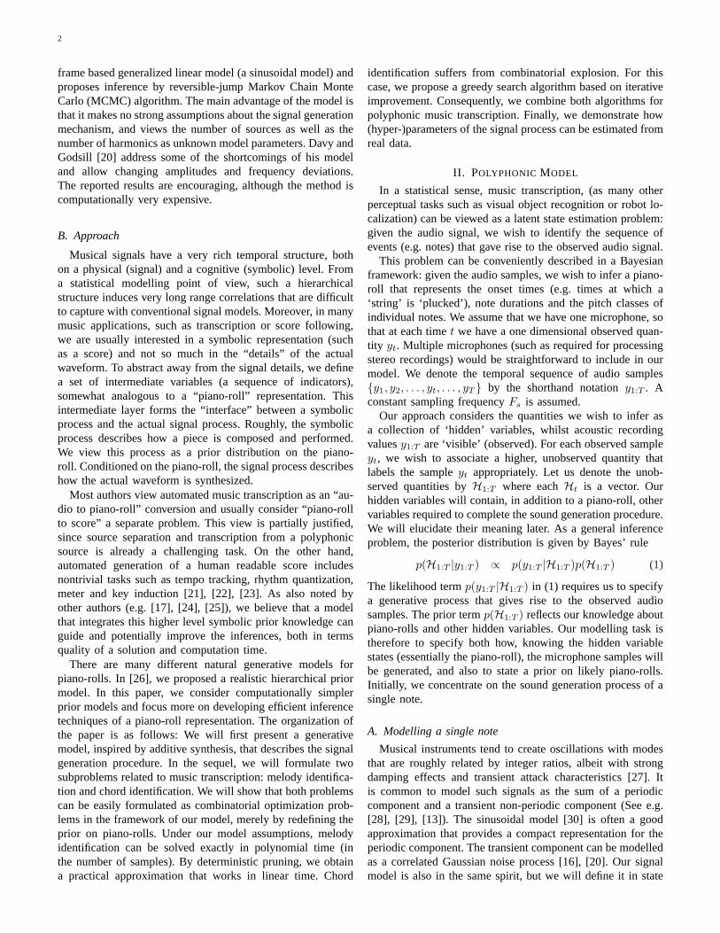
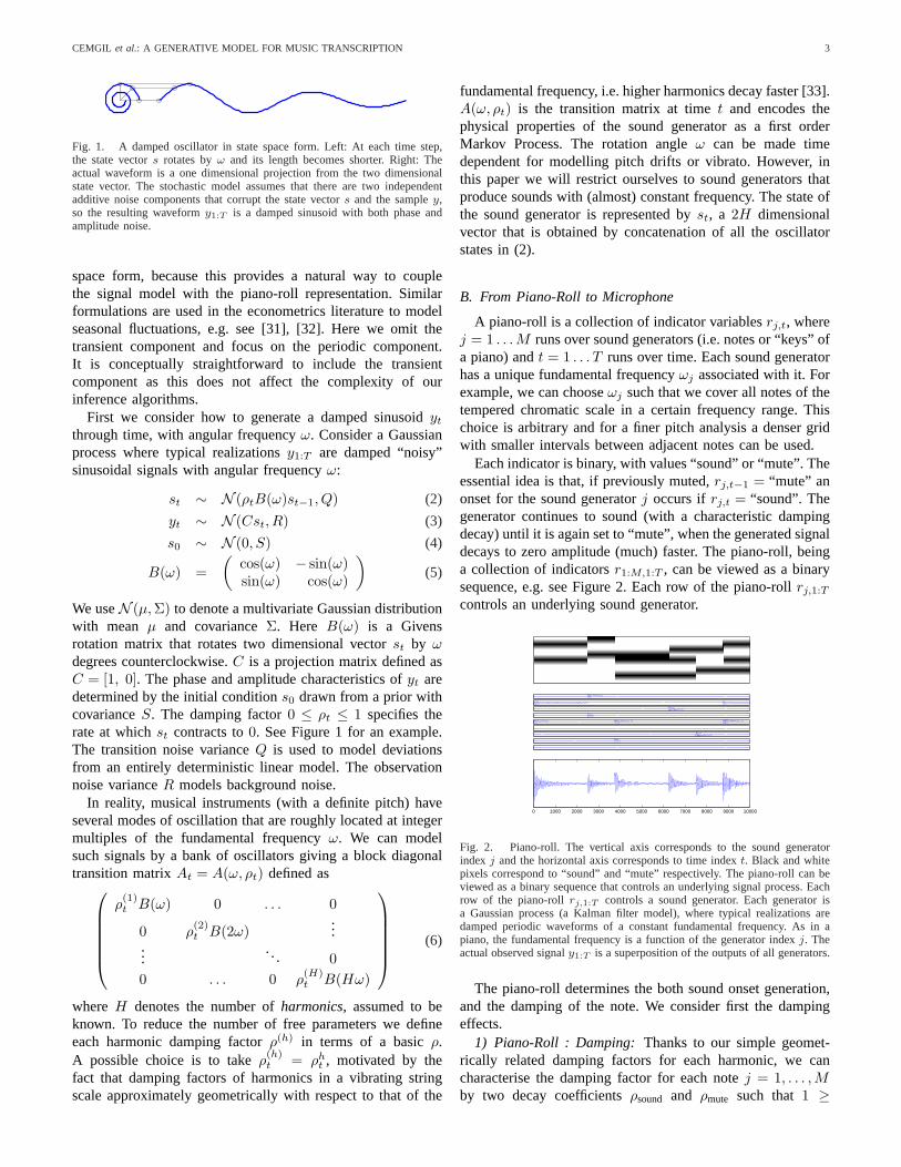
Fig. 1. A damped oscillator in state space form. Left: At each time step,the state vectors rotates byω and its length becomes shorter. Right: Theactual waveform is a one dimensional projection from the two dimensionalstate vector. The stochastic model assumes that there are two independentadditive noise components that corrupt the state vectors and the sampley,so the resulting waveformy1:T is a damped sinusoid with both phase andamplitude noise.

space form, because this provides a natural way to couplethe signal model with the piano-roll representation. Similarformulations are used in the econometrics literature to modelseasonal fluctuations, e.g. see [31], [32]. Here we omit thetransient component and focus on the periodic component.It is conceptually straightforward to include the transientcomponent as this does not affect the complexity of ourinference algorithms.

First we consider how to generate a damped sinusoidyt

through time, with angular frequencyω. Consider a Gaussianprocess where typical realizationsy1:T are damped “noisy”sinusoidal signals with angular frequencyω:

st ∼ N (ρtB(ω)st−1, Q) (2)

yt ∼ N (Cst, R) (3)

s0 ∼ N (0, S) (4)

B(ω) =(

cos(ω) − sin(ω)sin(ω) cos(ω)

)(5)

We useN (µ, Σ) to denote a multivariate Gaussian distributionwith mean µ and covarianceΣ. Here B(ω) is a Givensrotation matrix that rotates two dimensional vectorst by ωdegrees counterclockwise.C is a projection matrix defined asC = [1, 0]. The phase and amplitude characteristics ofyt aredetermined by the initial conditions0 drawn from a prior withcovarianceS. The damping factor0 ≤ ρt ≤ 1 specifies therate at whichst contracts to0. See Figure 1 for an example.The transition noise varianceQ is used to model deviationsfrom an entirely deterministic linear model. The observationnoise varianceR models background noise.

In reality, musical instruments (with a definite pitch) haveseveral modes of oscillation that are roughly located at integermultiples of the fundamental frequencyω. We can modelsuch signals by a bank of oscillators giving a block diagonaltransition matrixAt = A(ω, ρt) defined as

ρ(1)t B(ω) 0 . . . 0

0 ρ(2)t B(2ω)

......

. .. 00 . . . 0 ρ

(H)t B(Hω)

(6)

where H denotes the number ofharmonics, assumed to beknown. To reduce the number of free parameters we defineeach harmonic damping factorρ(h) in terms of a basicρ.A possible choice is to takeρ(h)

t = ρht , motivated by the

fact that damping factors of harmonics in a vibrating stringscale approximately geometrically with respect to that of the

fundamental frequency, i.e. higher harmonics decay faster [33].A(ω, ρt) is the transition matrix at timet and encodes thephysical properties of the sound generator as a first orderMarkov Process. The rotation angleω can be made timedependent for modelling pitch drifts or vibrato. However, inthis paper we will restrict ourselves to sound generators thatproduce sounds with (almost) constant frequency. The state ofthe sound generator is represented byst, a 2H dimensionalvector that is obtained by concatenation of all the oscillatorstates in (2).

B. From Piano-Roll to Microphone

A piano-roll is a collection of indicator variablesrj,t, wherej = 1 . . .M runs over sound generators (i.e. notes or “keys” ofa piano) andt = 1 . . . T runs over time. Each sound generatorhas a unique fundamental frequencyωj associated with it. Forexample, we can chooseωj such that we cover all notes of thetempered chromatic scale in a certain frequency range. Thischoice is arbitrary and for a finer pitch analysis a denser gridwith smaller intervals between adjacent notes can be used.

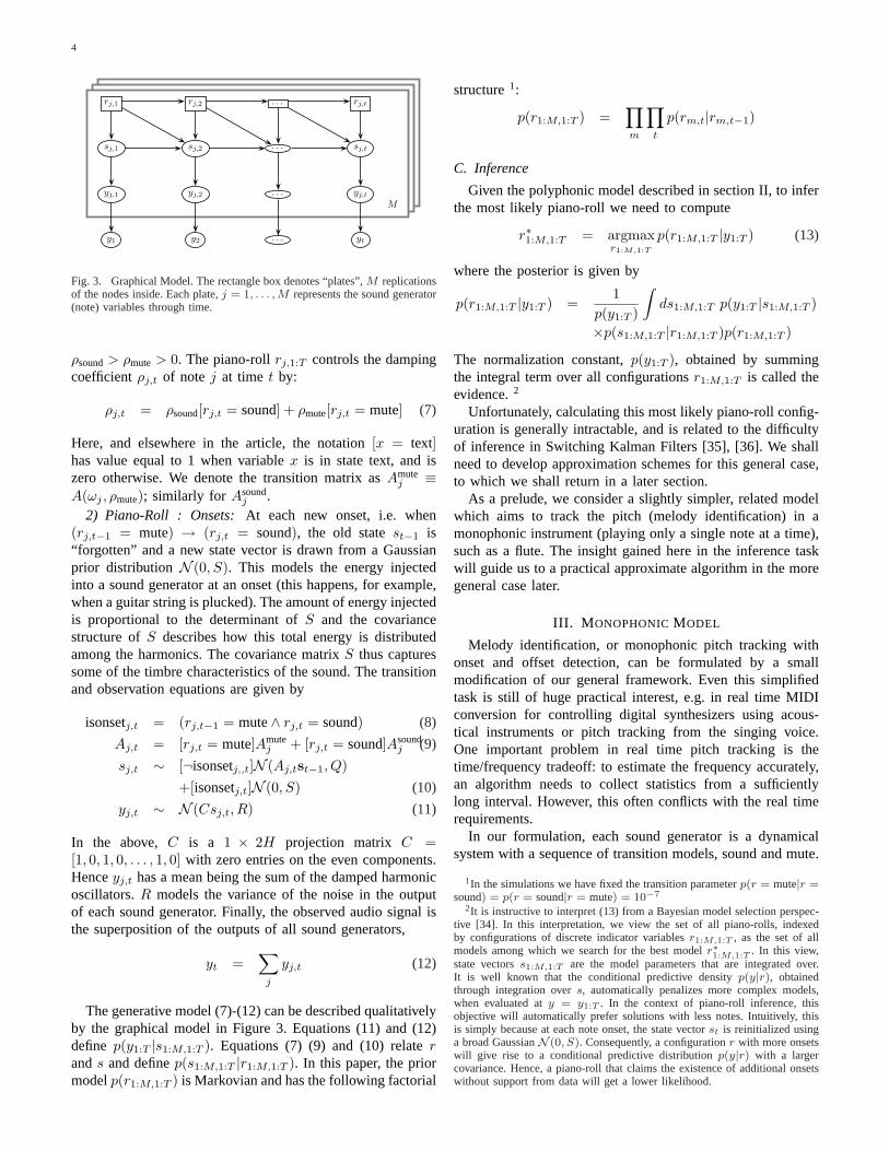
Each indicator is binary, with values “sound” or “mute”. Theessential idea is that, if previously muted,rj,t−1 = “mute” anonset for the sound generatorj occurs ifrj,t = “sound”. Thegenerator continues to sound (with a characteristic dampingdecay) until it is again set to “mute”, when the generated signaldecays to zero amplitude (much) faster. The piano-roll, beinga collection of indicatorsr1:M,1:T , can be viewed as a binarysequence, e.g. see Figure 2. Each row of the piano-rollrj,1:T

controls an underlying sound generator.

0 1000 2000 3000 4000 5000 6000 7000 8000 9000 10000

Fig. 2. Piano-roll. The vertical axis corresponds to the sound generatorindex j and the horizontal axis corresponds to time indext. Black and whitepixels correspond to “sound” and “mute” respectively. The piano-roll can beviewed as a binary sequence that controls an underlying signal process. Eachrow of the piano-rollrj,1:T controls a sound generator. Each generator isa Gaussian process (a Kalman filter model), where typical realizations aredamped periodic waveforms of a constant fundamental frequency. As in apiano, the fundamental frequency is a function of the generator indexj. Theactual observed signaly1:T is a superposition of the outputs of all generators.

The piano-roll determines the both sound onset generation,and the damping of the note. We consider first the dampingeffects.

1) Piano-Roll : Damping:Thanks to our simple geomet-rically related damping factors for each harmonic, we cancharacterise the damping factor for each notej = 1, . . . ,Mby two decay coefficientsρsound and ρmute such that1 ≥

4

M

rj,1 rj,2 . . . rj,t

sj,1 sj,2 . . . sj,t

yj,1 yj,2 . . . yj,t

y1 y2 . . . yt

Fig. 3. Graphical Model. The rectangle box denotes “plates”,M replicationsof the nodes inside. Each plate,j = 1, . . . , M represents the sound generator(note) variables through time.

ρsound> ρmute > 0. The piano-rollrj,1:T controls the dampingcoefficientρj,t of note j at time t by:

ρj,t = ρsound[rj,t = sound] + ρmute[rj,t = mute] (7)

Here, and elsewhere in the article, the notation[x = text]has value equal to 1 when variablex is in state text, and iszero otherwise. We denote the transition matrix asAmute

j ≡A(ωj , ρmute); similarly for Asound

j .2) Piano-Roll : Onsets: At each new onset, i.e. when

(rj,t−1 = mute) → (rj,t = sound), the old statest−1 is“forgotten” and a new state vector is drawn from a Gaussianprior distributionN (0, S). This models the energy injectedinto a sound generator at an onset (this happens, for example,when a guitar string is plucked). The amount of energy injectedis proportional to the determinant ofS and the covariancestructure ofS describes how this total energy is distributedamong the harmonics. The covariance matrixS thus capturessome of the timbre characteristics of the sound. The transitionand observation equations are given by

isonsetj,t = (rj,t−1 = mute∧ rj,t = sound) (8)

Aj,t = [rj,t = mute]Amutej + [rj,t = sound]Asound

j (9)

sj,t ∼ [¬isonsetj,,t]N (Aj,tst−1, Q)+[isonsetj,t]N (0, S) (10)

yj,t ∼ N (Csj,t, R) (11)

In the above,C is a 1 × 2H projection matrix C =[1, 0, 1, 0, . . . , 1, 0] with zero entries on the even components.Henceyj,t has a mean being the sum of the damped harmonicoscillators.R models the variance of the noise in the outputof each sound generator. Finally, the observed audio signal isthe superposition of the outputs of all sound generators,

yt =∑

j

yj,t (12)

The generative model (7)-(12) can be described qualitativelyby the graphical model in Figure 3. Equations (11) and (12)define p(y1:T |s1:M,1:T ). Equations (7) (9) and (10) relaterands and definep(s1:M,1:T |r1:M,1:T ). In this paper, the priormodelp(r1:M,1:T ) is Markovian and has the following factorial

structure1:

p(r1:M,1:T ) =∏m

∏t

p(rm,t|rm,t−1)

C. Inference

Given the polyphonic model described in section II, to inferthe most likely piano-roll we need to compute

r∗1:M,1:T = argmaxr1:M,1:T

p(r1:M,1:T |y1:T ) (13)

where the posterior is given by

p(r1:M,1:T |y1:T ) =1

p(y1:T )

∫ds1:M,1:T p(y1:T |s1:M,1:T )

×p(s1:M,1:T |r1:M,1:T )p(r1:M,1:T )

The normalization constant,p(y1:T ), obtained by summingthe integral term over all configurationsr1:M,1:T is called theevidence.2

Unfortunately, calculating this most likely piano-roll config-uration is generally intractable, and is related to the difficultyof inference in Switching Kalman Filters [35], [36]. We shallneed to develop approximation schemes for this general case,to which we shall return in a later section.

As a prelude, we consider a slightly simpler, related modelwhich aims to track the pitch (melody identification) in amonophonic instrument (playing only a single note at a time),such as a flute. The insight gained here in the inference taskwill guide us to a practical approximate algorithm in the moregeneral case later.

III. M ONOPHONICMODEL

Melody identification, or monophonic pitch tracking withonset and offset detection, can be formulated by a smallmodification of our general framework. Even this simplifiedtask is still of huge practical interest, e.g. in real time MIDIconversion for controlling digital synthesizers using acous-tical instruments or pitch tracking from the singing voice.One important problem in real time pitch tracking is thetime/frequency tradeoff: to estimate the frequency accurately,an algorithm needs to collect statistics from a sufficientlylong interval. However, this often conflicts with the real timerequirements.

In our formulation, each sound generator is a dynamicalsystem with a sequence of transition models, sound and mute.

1In the simulations we have fixed the transition parameterp(r = mute|r =sound) = p(r = sound|r = mute) = 10−7

2It is instructive to interpret (13) from a Bayesian model selection perspec-tive [34]. In this interpretation, we view the set of all piano-rolls, indexedby configurations of discrete indicator variablesr1:M,1:T , as the set of allmodels among which we search for the best modelr∗1:M,1:T . In this view,state vectorss1:M,1:T are the model parameters that are integrated over.It is well known that the conditional predictive densityp(y|r), obtainedthrough integration overs, automatically penalizes more complex models,when evaluated aty = y1:T . In the context of piano-roll inference, thisobjective will automatically prefer solutions with less notes. Intuitively, thisis simply because at each note onset, the state vectorst is reinitialized usinga broad GaussianN (0, S). Consequently, a configurationr with more onsetswill give rise to a conditional predictive distributionp(y|r) with a largercovariance. Hence, a piano-roll that claims the existence of additional onsetswithout support from data will get a lower likelihood.


The states evolves first according to the sounding regimewith transition matrixAsound and then according to the mutedregime withAmute. The important difference from a generalswitching Kalman filter is that when the indicatorr switchesfrom mute to sound, the old state vector is “forgotten”. Byexploiting this fact, in the appendix I-A we derive, for a singlesound generator (i.e. a single note of a fixed pitch that gets onand off), an exact polynomial time algorithm for calculatingthe evidencep(y1:T ) and MAP configurationr∗1:T .

1) Monophonic pitch tracking:Here we assume that at anygiven timet only a single sound generator can be sounding,i.e. rj,t = sound ⇒ rj′,t = mute for j′ 6= j. Hence,for practical purposes, the factorial structure of our originalmodel is redundant; i.e. we can “share” a single state vectors among all sound generators3. The resulting model will havethe same graphical structure as a single sound generator butwith an indicatorjt ∈ 1 . . . M which indexes the active soundgenerator, andrt ∈ {sound, mute} indicates sound or mute.Inference for this case turns out to be also tractable (i.e.polynomial). We allow switching to a newj′ only after anonset. The full generative model using the pairs(jt, rt), whichincludes both likelihood and prior terms is given as

rt ∼ p(rt|rt−1)isonsett = (rt = sound∧ rt−1 = mute)

jt ∼ [¬isonsett]δ(jt; jt−1) + [isonsett]u(jt)At = [rt = mute]Amute

jt+ [rt = sound]Asound

jt

st ∼ [¬isonsett]N (Atst−1, Q) + [isonsett]N (0, S)yt ∼ N (Cst, R)

Here u(j) denotes a uniform distribution on1, . . . , M andδ(jt; jt−1) denotes a degenerate (deterministic) distributionconcentrated onjt, i.e. unless there is an onset the active soundgenerator stays the same. Our choice of a uniformu(j) simplyreflects the fact that any new note is as likely as any other.Clearly, more informative priors, e.g. that reflect knowledgeabout tonality, can also be proposed. Similarly, for doing amore precise pitch analysis, we may choose a finer grid suchthat ωj+1/ωj = Q. Here,Q is the quality factor, a measureof the desired frequency precision not to be confused with thetransition noiseQ.

The graphical model is shown in Figure 4. The derivation ofthe polynomial time inference algorithm is given in appendix I-C. Technically, it is a simple extension of the single notealgorithm derived in appendix I-A.

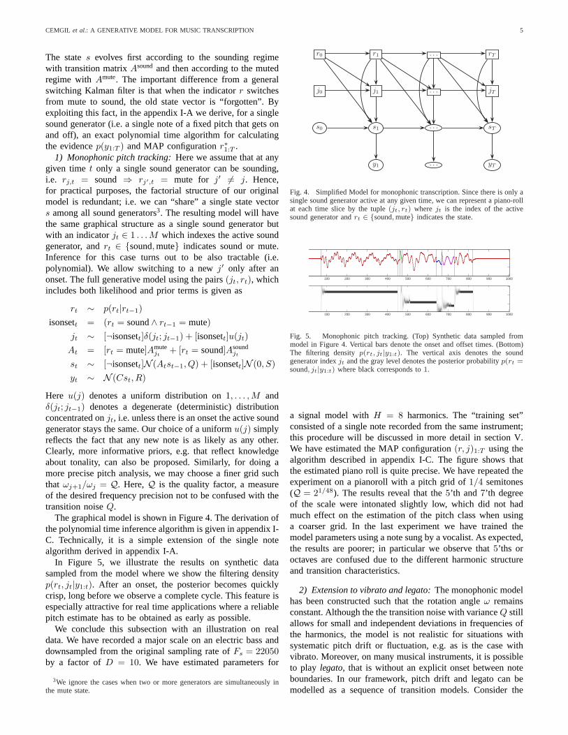
In Figure 5, we illustrate the results on synthetic datasampled from the model where we show the filtering densityp(rt, jt|y1:t). After an onset, the posterior becomes quicklycrisp, long before we observe a complete cycle. This feature isespecially attractive for real time applications where a reliablepitch estimate has to be obtained as early as possible.

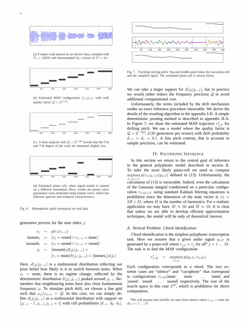
We conclude this subsection with an illustration on realdata. We have recorded a major scale on an electric bass anddownsampled from the original sampling rate ofFs = 22050by a factor ofD = 10. We have estimated parameters for

3We ignore the cases when two or more generators are simultaneously inthe mute state.

r0 r1 . . . rT

j0 j1 . . . jT

s0 s1. . . sT

y1 . . . yT

Fig. 4. Simplified Model for monophonic transcription. Since there is only asingle sound generator active at any given time, we can represent a piano-rollat each time slice by the tuple(jt, rt) where jt is the index of the activesound generator andrt ∈ {sound, mute} indicates the state.

100 200 300 400 500 600 700 800 900 1000

100 200 300 400 500 600 700 800 900 1000

Fig. 5. Monophonic pitch tracking. (Top) Synthetic data sampled frommodel in Figure 4. Vertical bars denote the onset and offset times. (Bottom)The filtering densityp(rt, jt|y1:t). The vertical axis denotes the soundgenerator indexjt and the gray level denotes the posterior probabilityp(rt =sound, jt|y1:t) where black corresponds to1.

a signal model withH = 8 harmonics. The “training set”consisted of a single note recorded from the same instrument;this procedure will be discussed in more detail in section V.We have estimated the MAP configuration(r, j)1:T using thealgorithm described in appendix I-C. The figure shows thatthe estimated piano roll is quite precise. We have repeated theexperiment on a pianoroll with a pitch grid of1/4 semitones(Q = 21/48). The results reveal that the5’th and 7’th degreeof the scale were intonated slightly low, which did not hadmuch effect on the estimation of the pitch class when usinga coarser grid. In the last experiment we have trained themodel parameters using a note sung by a vocalist. As expected,the results are poorer; in particular we observe that5’ths oroctaves are confused due to the different harmonic structureand transition characteristics.

2) Extension to vibrato and legato:The monophonic modelhas been constructed such that the rotation angleω remainsconstant. Although the the transition noise with varianceQ stillallows for small and independent deviations in frequencies ofthe harmonics, the model is not realistic for situations withsystematic pitch drift or fluctuation, e.g. as is the case withvibrato. Moreover, on many musical instruments, it is possibleto play legato, that is without an explicit onset between noteboundaries. In our framework, pitch drift and legato can bemodelled as a sequence of transition models. Consider the

6

(a) F major scale played on an electric bass, sampled withFs = 22050 and downsampled by a factor ofD = 10.

500 1000 1500 2000 2500 3000 3500

(b) Estimated MAP configuration(r, j)1:T with withquality factorQ = 21/12.

500 1000 1500 2000 2500 3000 3500

(c) A finer analysis withQ = 21/48 reveals that the 5’thand 7’th degree of the scale are intonated slightly low.

500 1000 1500 2000 2500 3000 3500

(d) Estimated piano roll, when signal model is trainedon a different instrument. Here, results are poorer sinceparameters were estimated using human voice, which hasdifferent spectral and temporal characteristics.

Fig. 6. Monophonic pitch estimation on real data.

generative process for the note indexj:

rt ∼ p(rt|rt−1)isonsett = (rt = sound∧ rt−1 = mute)issoundt = (rt = sound∧ rt−1 = sound)

jt ∼ [issoundt]d(jt|jt−1) +[rt = mute]δ(jt; jt−1) + [isonsett]u(jt)

Here, d(jt|jt−1) is a multinomial distribution reflecting ourprior belief how likely is it to switch between notes. Whenrt = mute, there is no regime change, reflected by thedeterministic distributionδ(jt; jt−1) peaked aroundjt−1. Re-member that neighbouring notes have also close fundamentalfrequencyω. To simulate pitch drift, we choose a fine gridsuch thatωj/ωj+1 = Q. In this case, we can simply de-fine d(jt|jt−1) as a multinomial distribution with support on[jt−1 − 1, jt−1, jt−1 + 1] with cell probabilities[d−1 d0 d1].

50 100 150 200 250 300 350 400 450 500

Fig. 7. Tracking varying pitch. Top and middle panel show the true piano-rolland the sampled signal. The estimated piano-roll is shown below.

We can take a larger support ford(jt|jt−1), but in practicewe would rather reduce the frequency precisionQ to avoidadditional computational cost.

Unfortunately, the terms included by the drift mechanismrender an exact inference procedure intractable. We derive thedetails of the resulting algorithm in the appendix I-D. A simpledeterministic pruning method is described in appendix II-A.In Figure 7, we show the estimated MAP trajectoryr∗1:T fordrifting pitch. We use a model where the quality factor isQ = 2−120, (120 generators per octave) with drift probabilityd−1 = d1 = 0.1. A fine pitch contour, that is accurate tosample precision, can be estimated.

IV. POLYPHONIC INFERENCE

In this section we return to the central goal of inferencein the general polyphonic model described in section II.To infer the most likely piano-roll we need to computeargmaxr1:M,1:T

p(r1:M,1:T |y1:T ) defined in (13). Unfortunately, the

calculation of (13) is intractable. Indeed, even the calculationof the Gaussian integral conditioned on a particular configu-ration r1:M,1:T using standard Kalman filtering equations isprohibitive since the dimension of the state vector is|s| =2H×M , whereH is the number of harmonics. For a realisticapplication we may haveM ≈ 50 and H ≈ 10. It is clearthat unless we are able to develop efficient approximationtechniques, the model will be only of theoretical interest.

A. Vertical Problem: Chord identification

Chord identification is the simplest polyphonic transcriptiontask. Here we assume that a given audio signaly1:T isgenerated by a piano-roll whererj,t = rj for all4 j = 1 . . .M .The task is to find the MAP configuration

r∗1:M = argmaxr1:M

p(y1:T , r1:M )

Each configuration corresponds to a chord. The two ex-treme cases are “silence” and “cacophony” that correspondto configurationsr1:M [mute mute . . . mute] and[sound sound . . . sound] respectively. The size of thesearch space in this case2M , which is prohibitive for directcomputation.

4We will assume that initially we start from silence whererj,0 = mute forall j = 1 . . . M


0 50 100 150 200 250 300 350 400−20

−10

0

10

20

0 π/4 π/2 3π/40

100

200

300

400

500

600

iteration r1 rM log p(y1:T , r1:M )

1 ◦ ◦ ◦ ◦ ◦ ◦ ◦ • ◦ ◦ ◦ ◦ ◦ ◦ ◦ ◦ ◦ ◦ ◦ ◦ ◦ ◦ ◦ ◦ −1220638254

2 ◦ ◦ ◦ ◦ ◦ ◦ ◦ • ◦ ◦ ◦ ◦ ◦ ◦ • ◦ ◦ ◦ ◦ ◦ ◦ ◦ ◦ ◦ −665073975

3 ◦ ◦ ◦ ◦ ◦ ◦ ◦ • ◦ ◦ ◦ ◦ ◦ ◦ • ◦ ◦ ◦ ◦ ◦ ◦ ◦ ◦ • −311983860

4 ◦ ◦ ◦ ◦ ◦ ◦ ◦ • ◦ ◦ ◦ ◦ ◦ ◦ • ◦ ◦ ◦ ◦ ◦ ◦ • ◦ • −162334351

5 ◦ ◦ ◦ ◦ ◦ ◦ ◦ • • ◦ ◦ ◦ ◦ ◦ • ◦ ◦ ◦ ◦ ◦ ◦ • ◦ • −43419569

6 ◦ ◦ ◦ ◦ ◦ ◦ ◦ • • ◦ ◦ ◦ ◦ ◦ • ◦ ◦ ◦ ◦ • ◦ • ◦ • −1633593

7 ◦ ◦ ◦ ◦ ◦ ◦ ◦ • • ◦ ◦ • ◦ ◦ • ◦ ◦ ◦ ◦ • ◦ • ◦ • −14336

8 ◦ ◦ ◦ ◦ ◦ ◦ ◦ • • ◦ • • ◦ ◦ • ◦ ◦ ◦ ◦ • ◦ • ◦ • −5766

9 ◦ ◦ ◦ ◦ ◦ ◦ ◦ • ◦ ◦ • • ◦ ◦ • ◦ ◦ ◦ ◦ • ◦ • ◦ • −5210

10 ◦ ◦ ◦ ◦ ◦ ◦ ◦ ◦ ◦ ◦ • • ◦ ◦ • ◦ ◦ ◦ ◦ • ◦ • ◦ • −4664

True ◦ ◦ ◦ ◦ ◦ ◦ ◦ ◦ ◦ ◦ • • ◦ ◦ • ◦ ◦ ◦ ◦ • ◦ • ◦ • −4664

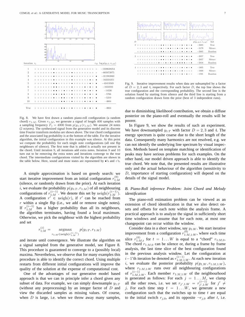
Fig. 8. We have first drawn a random piano-roll configuration (a randomchord)r1:M . Given r1:M , we generate a signal of length400 samples witha sampling frequencyFs = 4000 from p(y1:T |r1:M ). We assume 24 notes(2 octaves). The synthesized signal from the generative model and its discretetime Fourier transform modulus are shown above. The true chord configurationand the associated log probability is at the bottom of the table. For the iterativealgorithm, the initial configuration in this example was silence. At this pointwe compute the probability for each single note configurations (all one flipneighbours of silence). The first note that is added is actually not present inthe chord. Until iteration9, all iterations add extra notes. Iteration9 and10turn out to be removing the extra notes and iterations converge to the truechord. The intermediate configurations visited by the algorithm are shown inthe table below. Here, sound and mute states are represented by•’s and◦’s.

A simple approximation is based on greedy search: westart iterative improvement from an initial configurationr

(0)1:M

(silence, or randomly drawn from the prior). At each iterationi, we evaluate the probabilityp(y1:T , r1:M ) of all neighbouringconfigurations ofr(i−1)

1:M . We denote this set byneigh(r(i−1)1:M ).

A configuration r′ ∈ neigh(r), if r′ can be reached fromr within a single flip (i.e., we add or remove single notes).If r

(i−1)1:M has a higher probability than all its neighbours,

the algorithm terminates, having found a local maximum.Otherwise, we pick the neighbour with the highest probabilityand set

r(i)1:M = argmax

r1:M∈neigh(r(i−1)1:M )

p(y1:T , r1:M )

and iterate until convergence. We illustrate the algorithm ona signal sampled from the generative model, see Figure 8.This procedure is guaranteed to converge to a (possibly local)maxima. Nevertheless, we observe that for many examples thisprocedure is able to identify the correct chord. Using multiplerestarts from different initial configurations will improve thequality of the solution at the expense of computational cost.

One of the advantages of our generative model basedapproach is that we can in principle infer a chord given anysubset of data. For example, we can simply downsampley1:T

(without any preprocessing) by an integer factor ofD andview the discarded samples as missing values. Of course,when D is large, i.e. when we throw away many samples,

0 20 40 60 80 100 120 140 160 180 200−20

−10

0

10

20

0 π/4 π/2 3π/40

50

100

150

200

250

300

0 20 40 60 80 100 120 140−20

−15

−10

−5

0

5

10

15

0 π/4 π/2 3π/40

50

100

150

200

250

0 10 20 30 40 50 60 70 80 90 100−20

−10

0

10

20

0 π/4 π/2 3π/40

50

100

150

D p(y1:D:T , r1:M ) Init

2 ◦ ◦ ◦ ◦ ◦ ◦ ◦ ◦ ◦ ◦ • • ◦ ◦ • ◦ ◦ ◦ ◦ • ◦ • ◦ • −2685 True

◦ ◦ ◦ ◦ ◦ ◦ ◦ ◦ ◦ ◦ • ◦ ◦ • • ◦ ◦ • ◦ • ◦ • ◦ • −3179 Silence

◦ ◦ ◦ ◦ ◦ ◦ ◦ ◦ ◦ ◦ • • ◦ ◦ • ◦ ◦ ◦ ◦ • ◦ • ◦ • −2685 Random

3 ◦ ◦ ◦ ◦ ◦ ◦ ◦ ◦ ◦ ◦ • • ◦ ◦ • ◦ ◦ ◦ ◦ • ◦ • ◦ • −2057 True

◦ ◦ ◦ ◦ ◦ ◦ ◦ ◦ ◦ ◦ • • ◦ ◦ • ◦ ◦ ◦ ◦ • ◦ • ◦ • −2057 Silence

◦ ◦ ◦ ◦ ◦ ◦ ◦ ◦ ◦ • ◦ ◦ • ◦ • ◦ ◦ • • • • ◦ ◦ • −2616 Random

4 ◦ ◦ ◦ ◦ ◦ ◦ ◦ ◦ ◦ ◦ • • ◦ ◦ • ◦ ◦ ◦ ◦ • ◦ • ◦ • −1605 True

◦ ◦ ◦ ◦ ◦ ◦ ◦ ◦ • ◦ • • ◦ ◦ • ◦ • ◦ ◦ • ◦ ◦ ◦ ◦ −1668 Silence

◦ ◦ ◦ ◦ ◦ ◦ ◦ ◦ ◦ ◦ • • ◦ ◦ • ◦ ◦ ◦ ◦ • ◦ • ◦ ◦ −1591 Random

Fig. 9. Iterative improvement results when data are subsampled by a factorof D = 2, 3 and 4, respectively. For each factorD, the top line shows thetrue configuration and the corresponding probability. The second line is thesolution found by starting from silence and the third line is starting from arandom configuration drawn form the prior (best of3 independent runs).

due to diminishing likelihood contribution, we obtain a diffuseposterior on the piano-roll and eventually the results will bepoorer.

In Figure 9, we show the results of such an experiment.We have downsampledy1:T with factor D = 2, 3 and4. Theenergy spectrum is quite coarse due to the short length of thedata. Consequently many harmonics are not resolved, e.g. wecan not identify the underlying line spectrum by visual inspec-tion. Methods based on template matching or identification ofpeaks may have serious problems for such examples. On theother hand, our model driven approach is able to identify thetrue chord. We note that, the presented results are illustrativeonly and the actual behaviour of the algorithm (sensitivity toD, importance of starting configuration) will depend on thedetails of the signal model.

B. Piano-Roll inference Problem: Joint Chord and Melodyidentification

The piano-roll estimation problem can be viewed as anextension of chord identification in that we also detect on-sets and offsets for each note within the analysis frame. Apractical approach is to analyze the signal in sufficiently shorttime windows and assume that for each note, at most onechangepoint can occur within the window.

Consider data in a short window, sayy1:W . We start iterativeimprovement from a configurationr(0)

1:M,1:W , where each time

slice r(0)1:M,t for t = 1 . . . W is equal to a “chord”r1:M,0.

The chordr1:M,0 can be silence or, during a frame by frameanalysis, the last time slice of the best configuration foundin the previous analysis window. Let the configuration ati−1’th iteration be denoted asr(i−1)

1:M,1:W . At each new iterationi, we evaluate the posterior probabilityp(y1,W , r1:M,1:W ),where r1:M,1:W runs over all neighbouring configurationsof r

(i−1)1:M,1:W . Each memberr1:M,1:W of the neighbourhood

is generated as follows: For eachj = 1 . . . M , we clampall the other rows, i.e. we setrj′,1:W = r

(i−1)j′,1:W for j′ 6=

j. For each time stept = 1 . . . W , we generate a newconfiguration such that the switches up to timet are equalto the initial switchrj,0, and its opposite¬rj,0 after t, i.e.

8

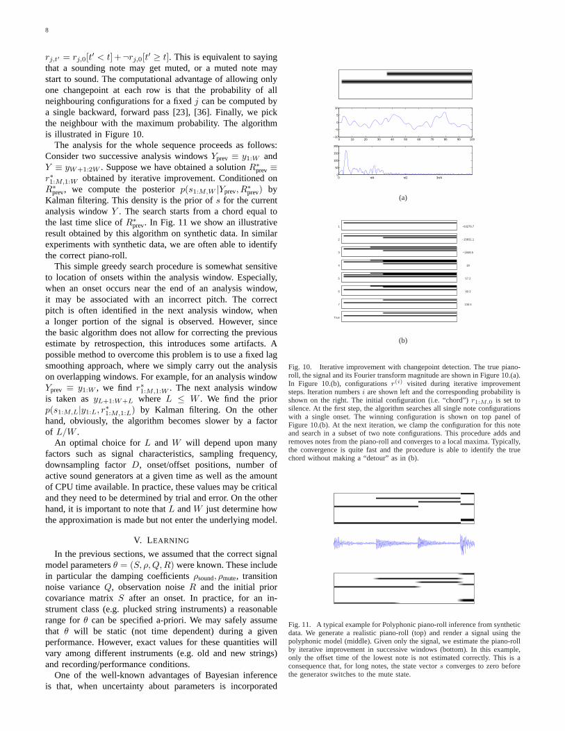
rj,t′ = rj,0[t′ < t]+¬rj,0[t′ ≥ t]. This is equivalent to sayingthat a sounding note may get muted, or a muted note maystart to sound. The computational advantage of allowing onlyone changepoint at each row is that the probability of allneighbouring configurations for a fixedj can be computed bya single backward, forward pass [23], [36]. Finally, we pickthe neighbour with the maximum probability. The algorithmis illustrated in Figure 10.

The analysis for the whole sequence proceeds as follows:Consider two successive analysis windowsYprev ≡ y1:W andY ≡ yW+1:2W . Suppose we have obtained a solutionR∗prev≡r∗1:M,1:W obtained by iterative improvement. Conditioned onR∗prev, we compute the posteriorp(s1:M,W |Yprev, R

∗prev) by

Kalman filtering. This density is the prior ofs for the currentanalysis windowY . The search starts from a chord equal tothe last time slice ofR∗prev. In Fig. 11 we show an illustrativeresult obtained by this algorithm on synthetic data. In similarexperiments with synthetic data, we are often able to identifythe correct piano-roll.

This simple greedy search procedure is somewhat sensitiveto location of onsets within the analysis window. Especially,when an onset occurs near the end of an analysis window,it may be associated with an incorrect pitch. The correctpitch is often identified in the next analysis window, whena longer portion of the signal is observed. However, sincethe basic algorithm does not allow for correcting the previousestimate by retrospection, this introduces some artifacts. Apossible method to overcome this problem is to use a fixed lagsmoothing approach, where we simply carry out the analysison overlapping windows. For example, for an analysis windowYprev ≡ y1:W , we find r∗1:M,1:W . The next analysis windowis taken asyL+1:W+L where L ≤ W . We find the priorp(s1:M,L|y1:L, r∗1:M,1:L) by Kalman filtering. On the otherhand, obviously, the algorithm becomes slower by a factorof L/W .

An optimal choice forL and W will depend upon manyfactors such as signal characteristics, sampling frequency,downsampling factorD, onset/offset positions, number ofactive sound generators at a given time as well as the amountof CPU time available. In practice, these values may be criticaland they need to be determined by trial and error. On the otherhand, it is important to note thatL andW just determine howthe approximation is made but not enter the underlying model.

V. L EARNING

In the previous sections, we assumed that the correct signalmodel parametersθ = (S, ρ, Q, R) were known. These includein particular the damping coefficientsρsound, ρmute, transitionnoise varianceQ, observation noiseR and the initial priorcovariance matrixS after an onset. In practice, for an in-strument class (e.g. plucked string instruments) a reasonablerange forθ can be specified a-priori. We may safely assumethat θ will be static (not time dependent) during a givenperformance. However, exact values for these quantities willvary among different instruments (e.g. old and new strings)and recording/performance conditions.

One of the well-known advantages of Bayesian inferenceis that, when uncertainty about parameters is incorporated

0 10 20 30 40 50 60 70 80 90 100−10

−5

0

5

10

0 π/4 π/2 3π/40

50

100

150

200

(a)

1 −63276.7

2 −15831.1

3 −1848.5

4 19

5 57.2

6 90.3

7 130.5

True

(b)

Fig. 10. Iterative improvement with changepoint detection. The true piano-roll, the signal and its Fourier transform magnitude are shown in Figure 10.(a).In Figure 10.(b), configurationsr(i) visited during iterative improvementsteps. Iteration numbersi are shown left and the corresponding probability isshown on the right. The initial configuration (i.e. “chord”)r1:M,0 is set tosilence. At the first step, the algorithm searches all single note configurationswith a single onset. The winning configuration is shown on top panel ofFigure 10.(b). At the next iteration, we clamp the configuration for this noteand search in a subset of two note configurations. This procedure adds andremoves notes from the piano-roll and converges to a local maxima. Typically,the convergence is quite fast and the procedure is able to identify the truechord without making a “detour” as in (b).

Fig. 11. A typical example for Polyphonic piano-roll inference from syntheticdata. We generate a realistic piano-roll (top) and render a signal using thepolyphonic model (middle). Given only the signal, we estimate the piano-rollby iterative improvement in successive windows (bottom). In this example,only the offset time of the lowest note is not estimated correctly. This is aconsequence that, for long notes, the state vectors converges to zero beforethe generator switches to the mute state.


in a model, this leads in a natural way to the formulationof a learning algorithm. The piano-roll estimation problem,omitting the time indices, can be stated as follows:

r∗ = argmaxr

∫dθ

∫ds p(y|s, θ)p(s|r, θ)p(θ)p(r) (14)

In other words, we wish to find the best piano-roll by takinginto account all possible settings of the parameterθ, weightedby the prior. Note that (14) becomes equivalent to (13), ifwe knew the “best” parameterθ∗, i.e. p(θ) = δ(θ − θ∗).Unfortunately, the integration onθ can not be calculatedanalytically and approximation methods must be used [37]. Acrude but computationally cheap approximation replaces theintegration onθ in (14) with maximization:

r∗ = argmaxr

maxθ

∫ds p(y|s, θ)p(s|r, θ)p(θ)p(r)

Essentially, this is a joint optimization problem on piano-rolls and parameters which we solve by a greedy coordinateascent algorithm. The algorithm we propose is a doubleloop algorithm where we iterate in the outer loop betweenmaximization overr and maximization overθ. The lattermaximization itself is calculated with an iterative algorithm:

r(i) = argmaxr

∫dsp(y|s, θ(i−1))p(s|r, θ(i−1))p(θ(i−1))p(r)

θ(i) = argmaxθ

∫dsp(y|s, θ)p(s|r(i), θ)p(θ)p(r(i))

For a single note, conditioned on a fixedθ(i−1), r(i) can becalculated exactly, using the message propagation algorithmderived in appendix I-B. Conditioned onr(i), maximization onthe θ coordinate becomes equivalent to parameter estimationin linear dynamical systems, for which no closed form solutionis known. Nevertheless, this step can be calculated by an iter-ative expectation maximization (EM) algorithm [36], [38]. Inpractice, we observe that for realistic starting conditionsθ(0),the r(i) are identical, suggesting that the best segmentationr∗

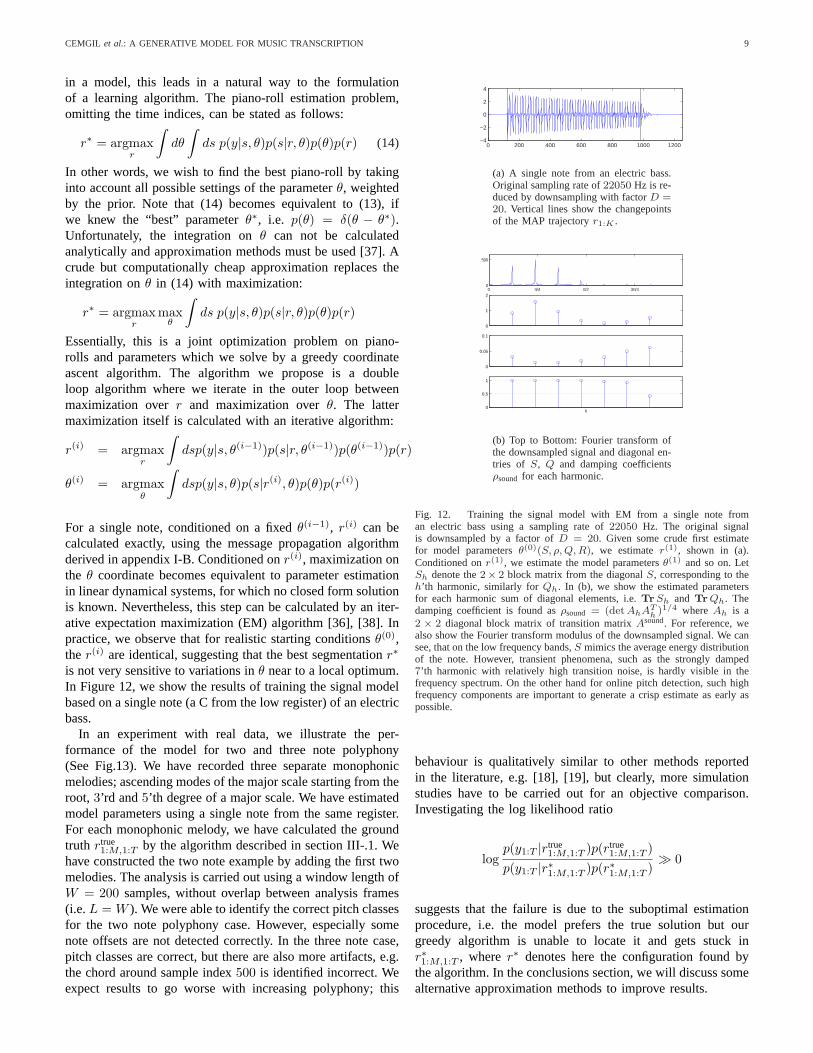
is not very sensitive to variations inθ near to a local optimum.In Figure 12, we show the results of training the signal modelbased on a single note (a C from the low register) of an electricbass.

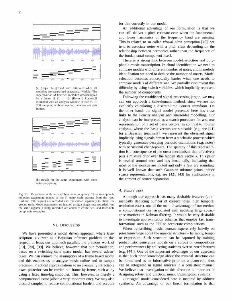
In an experiment with real data, we illustrate the per-formance of the model for two and three note polyphony(See Fig.13). We have recorded three separate monophonicmelodies; ascending modes of the major scale starting from theroot,3’rd and5’th degree of a major scale. We have estimatedmodel parameters using a single note from the same register.For each monophonic melody, we have calculated the groundtruth rtrue

1:M,1:T by the algorithm described in section III-.1. Wehave constructed the two note example by adding the first twomelodies. The analysis is carried out using a window length ofW = 200 samples, without overlap between analysis frames(i.e.L = W ). We were able to identify the correct pitch classesfor the two note polyphony case. However, especially somenote offsets are not detected correctly. In the three note case,pitch classes are correct, but there are also more artifacts, e.g.the chord around sample index500 is identified incorrect. Weexpect results to go worse with increasing polyphony; this

0 200 400 600 800 1000 1200−4

−2

0

2

4

(a) A single note from an electric bass.Original sampling rate of22050 Hz is re-duced by downsampling with factorD =20. Vertical lines show the changepointsof the MAP trajectoryr1:K .

0 π/4 π/2 3π/40

500

0

1

2

0

0.05

0.1

0

0.5

1

h

(b) Top to Bottom: Fourier transform ofthe downsampled signal and diagonal en-tries of S, Q and damping coefficientsρsound for each harmonic.

Fig. 12. Training the signal model with EM from a single note froman electric bass using a sampling rate of22050 Hz. The original signalis downsampled by a factor ofD = 20. Given some crude first estimatefor model parametersθ(0)(S, ρ, Q, R), we estimater(1), shown in (a).Conditioned onr(1), we estimate the model parametersθ(1) and so on. LetSh denote the2× 2 block matrix from the diagonalS, corresponding to theh’th harmonic, similarly forQh. In (b), we show the estimated parametersfor each harmonic sum of diagonal elements, i.e.TrSh and TrQh. Thedamping coefficient is found asρsound = (det AhAT

h )1/4 where Ah is a2 × 2 diagonal block matrix of transition matrixAsound. For reference, wealso show the Fourier transform modulus of the downsampled signal. We cansee, that on the low frequency bands,S mimics the average energy distributionof the note. However, transient phenomena, such as the strongly damped7’th harmonic with relatively high transition noise, is hardly visible in thefrequency spectrum. On the other hand for online pitch detection, such highfrequency components are important to generate a crisp estimate as early aspossible.

behaviour is qualitatively similar to other methods reportedin the literature, e.g. [18], [19], but clearly, more simulationstudies have to be carried out for an objective comparison.Investigating the log likelihood ratio

logp(y1:T |rtrue

1:M,1:T )p(rtrue1:M,1:T )

p(y1:T |r∗1:M,1:T )p(r∗1:M,1:T )À 0

suggests that the failure is due to the suboptimal estimationprocedure, i.e. the model prefers the true solution but ourgreedy algorithm is unable to locate it and gets stuck inr∗1:M,1:T , wherer∗ denotes here the configuration found bythe algorithm. In the conclusions section, we will discuss somealternative approximation methods to improve results.

10

500 1000 1500 2000 2500 3000

500 1000 1500 2000 2500 3000

500 1000 1500 2000 2500 3000

(a) (Top) The ground truth estimated when allmelodies are transcribed separately. (Middle) Thesuperposition of first two melodies downsampledby a factor of D = 10. (Bottom) Piano-rollestimated with an analysis window of sizeW =200 samples, without overlap between analysisframes.

500 1000 1500 2000 2500 3000

500 1000 1500 2000 2500 3000

500 1000 1500 2000 2500 3000

(b) Result for the same experiment with threenotes polyphony.

Fig. 13. Experiment with two and three note polyphony. Three monophonicmelodies (ascending modes of the F major scale starting from the root,3’rd and 5’th degree) are recorded and transcribed separately to obtain theground truth. Model parameters are learned using a single note recorded fromthe same register. Finally, melodies are added to create two- and three-notepolyphonic examples.

VI. D ISCUSSION

We have presented a model driven approach where tran-scription is viewed as a Bayesian inference problem. In thisrespect, at least, our approach parallels the previous work of[19], [20], [39]. We believe, however, that our formulation,based on a switching state space model, has several advan-tages. We can remove the assumption of a frame based modeland this enables us to analyse music online and to sampleprecision. Practical approximations to an eventually intractableexact posterior can be carried out frame-by-frame, such as byusing a fixed time-lag smoother. This, however, is merely acomputational issue (albeit a very important one). We may alsodiscard samples to reduce computational burden, and account

for this correctly in our model.An additional advantage of our formulation is that we

can still deliver a pitch estimate even when the fundamentaland lower harmonics of the frequency band are missing.This is related to so calledvirtual pitch perception [40]: wetend to associate notes with a pitch class depending on therelationship between harmonics rather than the frequency ofthe fundamental component itself.

There is a strong link between model selection and poly-phonic music transcription. In chord identification we need tocompare models with different number of notes, and in melodyidentification we need to deduce the number of onsets. Modelselection becomes conceptually harder when one needs tocompare models of different size. We partially circumvent thisdifficulty by using switch variables, which implicitly representthe number of components.

Following the established signal processing jargon, we maycall our approach a time-domain method, since we are notexplicitly calculating a discrete-time Fourier transform. Onthe other hand, the signal model presented here has closelinks to the Fourier analysis and sinusoidal modelling. Ouranalysis can be interpreted as a search procedure for a sparserepresentation on a set of basis vectors. In contrast to Fourieranalysis, where the basis vectors are sinusoids (e.g. see [41]for a Bayesian treatment), we represent the observed signalimplicitly using signals drawn from a stochastic process whichtypically generates decaying periodic oscillations (e.g. notes)with occasional changepoints. The sparsity of this representa-tion is a consequence of the onset mechanism, that effectivelyputs a mixture prior over the hidden state vectors. This prioris peaked around zero and has broad tails, indicating thatmost of the sources are muted and only a few are sounding.It is well known that such Gaussian mixture priors inducesparse representations, e.g. see [42], [43] for applications inthe context of source separation.

A. Future work

Although our approach has many desirable features (auto-matically deducing number of correct notes, high temporalresolution e.t.c.), one of the main disadvantage of our methodis computational cost associated with updating large covari-ance matrices in Kalman filtering. It would be very desirableto investigate approximation schemas that employ fast trans-formations such as the FFT to accelerate computations.

When transcribing music, human experts rely heavily onprior knowledge about the musical structure – harmony, tempoor expression. Such structure can be captured by trainingprobabilistic generative models on a corpus of compositionsand performances by collecting statistics over selected features(e.g. [44]). One of the important advantages of our approachis that such prior knowledge about the musical structure canbe formulated as an informative prior on a piano-roll; thuscan be integrated in signal analysis in a consistent manner.We believe that investigation of this direction is important indesigning robust and practical music transcription systems.

Our signal model considered here is inspired by additivesynthesis. An advantage of our linear formulation is that


we can use the Kalman filter recursions to integrate out thecontinuous latent state analytically. An alternative would beto formulate a nonlinear dynamical system that implementsa nonlinear synthesis model (e.g. FM synthesis, waveshapingsynthesis, or even a physical model[45]). Such an approachwould reduce the dimensionality of the latent state spacebut force us to use approximate integration methods such asparticle filters or EKF/UKF [46]. It remains an interesting openquestion whether, in practice, one should trade-off analyticaltractability versus reduced latent state dimension.

In this paper, for polyphonic transcription, we have useda relatively simple deterministic inference method based oniterative improvement. The basic greedy algorithm, whilst stillpotentially useful in practice, may get stuck in poor solutions.We believe that, using our model as a framework, better poly-phonic transcriptions can be achieved using more elaborateinference or search methods. For example, computation timeassociated with exhaustive search of the neighbourhood for allvisited configuations could be significantly reduced by ran-domizing the local search (e.g. by Metropolis-Hastings moves5 ) or use heuristic proposal distributions derived from easy-to-compute features such as the energy spectrum. Alternatively,sequential Monte Carlo methods or deterministic messagepropagation algorithms such as Expectation propagation (EP)[47] could be also used.

We have not yet tested our model for more general scenar-ios, such as music fragments containing percussive instrumentsor bell sounds with inharmonic spectra. Our simple periodicsignal model would be clearly inadequate for such a scenario.On the other hand, we stress the fact that the frameworkpresented here is not limited to the analysis of signals withharmonic spectra, and in principle applicable to any familyof signals that can be represented by a switching state spacemodel. This is already a large class since many real-worldacoustic processes can be approximated well with piecewiselinear regimes. We can also formulate a joint estimationschema for unknown parameters as in (14) and integratethem out (e.g. see [20]). However, this is currently a hardand computationally expensive task. If efficient and accurateapproximate integration methods can be developed, our modelwill be applicable to mixtures of many different types ofacoustical signals and may be useful in more general auditoryscene analysis problems.

1) Acknowledgments:This research is supported by theTechnology Foundation STW, applied science division ofNWO and the technology programme of the Dutch Ministry ofEconomic Affairs. We would like to thank the the anonymousreviewers for their comments and suggestions.

APPENDIX IDERIVATION OF MESSAGE PROPAGATION ALGORITHMS

In the appendix, we derive several exact message propaga-tion algorithms. Our derivation closely follows the standardderivation of recursive prediction and update equations forthe Kalman filter [48]. First we focus on a single soundgenerator. In appendix I-A and I-B, we derive polynomial

5This improvement is suggested by one of the anonymous reviewers

time algorithms for calculating the evidencep(y1:T ) and MAPconfigurationr∗1:T = argmax

r1:T

p(y1:T , r1:T ) respectively. The

MAP configuration is useful for onset/offset detection. Inthe following section, we extend the onset/offset detectionalgorithms to monophonic pitch tracking with constant fre-quency. We derive a polynomial time algorithm for this casein appendix I-C. The case for varying fundamental frequencyis derived in the following appendix I-D. In appendix II wedescribe heuristics to reduce the amount of computations.

A. Computation of the evidencep(y1:T ) for a single soundgenerator by forward filtering

We assume a Markovian prior on the indicatorsrt wherep(rt = i|rt−1 = j) ≡ pi,j . For convenience, we repeat thegenerative model for a single sound generator by omitting thenote indexj.

rt ∼ p(rt|rt−1)isonsett = (rt = sound∧ rt−1 = mute)

st ∼ [¬isonsett]N (Artst−1, Q) + [isonsett]N (0, S)

yt ∼ N (Cst, R)

For simplicity, we will sometime use the labels1 and 2to denote sound and mute respectively. We enumerate thetransition models asfrt(st|st−1) = N (Artst−1, Q). Wedefine the filtering potential as

αt ≡ p(y1:t, st, rt, rt−1) =∑

r1:t−2

∫ds0:t−1p(y1:t, s0:t, r1:t)

We assume thaty is always observed, hence we use the termpotential to indicate the fact thatp(y1:t, st, rt, rt−1) is notnormalized. The filtering potential is in general a conditionalGaussian mixture, i.e. a mixture of Gaussians for each con-figuration of rt−1:t. We will highlight this data structure byusing the following notation

αt ≡{

α1,1t α1,2

t

α2,1t α2,2

t

}

where eachαi,jt = p(y1:t, st, rt = i, rt−1 = j) for i, j =

1 . . . 2 are also Gaussian mixture potentials. We will denotethe conditional normalization constants as

Zit ≡ p(y1:t, rt = i) =

∑rt−1

∫dstα

i,rt−1t

Consequently the evidence is given by

Zt ≡ p(y1:t) =∑rt

∑rt−1

∫dstαt =

∑

i

Zit

We also define the predictive density

αt|t−1 ≡ p(y1:t−1, st, rt, rt−1)

=∑rt−2

∫dst−1 p(st|st−1, rt, rt−1)p(rt|rt−1)αt−1

In general, for switching Kalman filters, calculating exactposterior features, such as the evidenceZt = p(y1:t), is nottractable. This is a consequence of the fact that the number of

12

mixture components to required to represent the exact filteringdensity αt grows exponentially with time stepk (i.e. oneGaussian for each of the exponentially many configurationsr1:t). Luckily, for the model we are considering here, thegrowth is polynomial ink only. See also [49].

To see this, suppose we have the filtering density availableat timet− 1 asαt−1. The transition models can be organizedalso in a table wherei’th row andj’th column correspond top(st|st−1, rt = i, rt−1 = j)

p(st|st−1, rt, rt−1) ={

f1(st|st−1) π(st)f2(st|st−1) f2(st|st−1)

}

Calculation of the predictive potential is straightforward.First, summation overrt−2 yields

∑rt−2

αt−1 ={

α1,1t−1 + α1,2

t−1

α2,1t−1 + α2,2

t−1

}≡

{ξ1t−1

ξ2t−1

}

Integration over st−1 and multiplication by p(rt|rt−1)yields the predictive potential

αt|t−1 ={

p1,1ψ11(st) p1,2Z

2t−1π(st)

p2,1ψ12(st) p2,2ψ

22(st)

}

where we define

Z2t−1 ≡

∫dst−1ξ

2t−1

ψji (st) ≡

∫dst−1fi(st|st−1)ξ

jt−1

The potentialsψji can be computed by applying the standard

Kalman prediction equations to each component ofξjt−1.

The updated potential is given byαt = p(yt|st)αt|t−1. Thisquantity can be computed by applying standard Kalman updateequations to each component ofαt|t−1.

From the above derivation, it is clear thatα1,2t has only

a single Gaussian component. This has the consequence thatthe number of Gaussian components inα1,1

t increases onlylinearly (the first row-sum termsξ1

t−1 propagated throughf1).The second row sum termξ2

t is more costly; it increasesat every time slice by the number of components inξ1

t−1.Since the size ofξ1

t−1 grows linearly, the size ofξ2t grows

quadratically with timet.

B. Computation of MAP configurationr∗1:TThe MAP state is defined as

r∗1:T = argmaxr1:T

∫ds0:T p(y1:T , s0:T , r1:T )

≡ argmaxr1:T

∫ds0:T φ(s0:T , r1:T )

For finding the MAP state, we replace summations overrt by maximization. One potential technical difficulty is that,unlike in the case for evidence calculation, maximization andintegration do not commute. Consider a conditional Gaussianpotential

φ(s, r) ≡ {φ(s, r = 1), φ(s, r = 2)}

whereφ(s, r) are Gaussian potentials for each configurationof r. We can compute the MAP configuration

r∗ = argmaxr

∫ds φ(s, r) = argmax

{Z1, Z2

}

whereZj =∫

ds φ(s, r = j). We evaluate the normalizationof each component (i.e. integrate over the continuous hiddenvariables first) and finally find the maximum of all normal-ization constants.

However, direct calculation ofr∗1:T is not feasible because ofexponential explosion in the number of distinct configurations.Fortunately, for our model, we can introduce a deterministicpruning schema that reduces the number of kernels to apolynomial order and meanwhile guarantees that we will nevereliminate the MAP configuration. This exact pruning methodhinges on the factorization of the posterior for the assignmentof variablesrt = 1, rt−1 = 2 (mute to sound transition) thatbreaks the direct link betweenst andst−1:

φ(s0:T , r1:t−2, rt−1 = 2, rt = 1, rt+1:T ) =φ(s0:t−1, r1:t−2, rt−1 = 2)φ(st:T , rt+1:T , rt = 1|rt−1 = 2)

(15)

In this case:

maxr1:T

∫ds0:T φ(s0:T , r1:t−2, rt−1 = 2, rt = 1, rt+1:T )

= maxr1:t−1

∫ds0:t−1 φ(s0:t−1, r1:t−2, rt−1 = 2)

×maxrt:T

∫dst:T φ(st:T , rt+1:T , rt = 1|rt−1 = 2)

= Z2t ×maxrt+1:T

∫dst:T φ(st:T , rt+1:T , rt = 1|rt−1 = 2)(16)

This Equation shows that whenever we have an onset,we can calculate the maximum over the past and futureconfigurations separately. Put differently, provided that theMAP configuration has the formr∗1:T = [r∗1:t−3, rt−1 =2, rt = 1, r∗t+1:T ], the prefix [r∗1:t−3, rt−1 = 2] willbe the solution for the reduced maximization problemarg maxr1:t−1

∫ds0:t−1 φ(s0:t−1, r1:t−1).

1) Forward pass:Suppose we have a collection of Gaussianpotentials

δt−1 ≡{

δ1,1t−1 δ1,2

t−1

δ2,1t−1 δ2,2

t−1

}≡

{δ1t−1

δ2t−1

}

with the property that the Gaussian kernel corresponding theprefix r∗1:t−1 of the MAP state is a member ofδt−1, i.e.φ(st−1, r

∗1:t−1) ∈ δt−1 s.t.r∗1:T = [r∗1:t−1, r

∗t:T ]. We also define

the subsets

δi,jt−1 = {φ(st−1, r1:t−1) : φ ∈ δt−1andrt−1 = i, rt−2 = j}

δit−1 =

⋃

j

δi,jt−1

We show how we findδt. The prediction is given by

δt|t−1 =∫

dst−1 p(st|st−1, rt, rt−1)p(rt|rt−1)δt−1

The multiplication byp(rt|rt−1) and integration overst−1

yields the predictive potentialδt|t−1

{p1,1

∫dst−1 f1(st|st−1)δ1

t−1 p1,2π(st)∫

dst−1 δ2t−1

p2,1


t−1 p2,2


t−1

}


By the (16), we can replace the collection of numbers∫dst−1 δ2

t−1 with with the scalarZ2t−1 ≡ max

∫dst−1 δ2

t−1

without changing the optimum solution:

δ1,2t|t−1 = p1,2Z

2t−1π(st)

The updated potential is given byδt = p(yt|st)δt|t−1. Theanalysis of the number of kernels proceeds as in the previoussection.

2) Decoding: During the forward pass, we tag each Gaus-sian component ofδt with its past history ofr1:t. The MAPstate can be found by a simple search in the collection ofpolynomially many numbers and reporting the associated tag:

r∗1:T = argmaxr1:T

∫dsT δT

We finally conclude that the forward filtering and MAP(Viterbi path) estimation algorithms are essentially identicalwith summation replaced by maximization and an additionaltagging required for decoding.

C. Inference for monophonic pitch tracking

In this section we derive an exact message propagationalgorithm for monophonic pitch tracking. Perhaps surprisingly,inference in this case turns out to be still tractable. Eventhough the size of the configuration spacer1:M,1:T is of size(M + 1)T = O(2T log M ), the space complexity of an exactalgorithm remains quadratic int. First, we define a “mega”indicator nodezt = (jt, rt) wherejt ∈ 1 . . .M indicates theindex of the active sound generator andrt ∈ {sound, mute}indicates its state. The transition modelp(zt|zt−1) is a largesparse transition table with probabilities

p1,1 p1,2/M . . . p1,2/M. ..

..... .

...p1,1 p1,2/M . . . p1,2/M

p2,1 p2,2

. .... .

p2,1 p2,2

(17)

where the transitionsp(zt = (j, r)|zt−1 = (j′, r′)) areorganized at then’th row and m’th column wheren =r × M + j − 1 and m = r′ × M + j′ − 1. (17). Thetransition modelsp(st|st−1, zt = (j, r), zt−1 = (j′, r′)) canbe organized similarly:

f1,1 π(st) . . . π(st).. .

.... ..

...f1,M π(st) . . . π(st)

f2,1 f2,1

.. .. ..

f2,M f2,M

Here, fr,j ≡ fr,j(st|st−1) denotes the transition model ofthe j’th sound generator when in stater. The derivation forfiltering follows the same lines as the onset/offset detectionmodel, with only slightly more tedious indexing. Suppose wehave the filtering density available at timet− 1 asαt−1. We

first calculate the predictive potential. Summation overzt−2

yields the row sums

ξ(r,j)t−1 =

∑

r′,j′α

(r,j),(r′,j′)t−1

Integration overst−1 and multiplication byp(zt|zt−1) yieldsthe predictive potentialαt|t−1. The components are given as

α(r,j)(r′,j′)t|t−1 =

{(1/M)pr,r′π(st)Z

(r′,j′)t−1 r = 1 ∧ r′ = 2

[j = j′]× pr,r′ψ(r,j)(r′,j′)t otherwise

(18)

where we define

Z(r′,j′)t−1 ≡

∫dst−1 ξ

(r′,j′)t−1

ψ(r,j)(r′,j′)t ≡

∫dst−1 fr,j(st|st−1)ξ

(r′,j′)t−1

The potentialsψ can be computed by applying the standardKalman prediction equations to each component ofξ. Notethat the forward messages have the same sparsity structure asthe prior, i.e.α(r,j)(r′,j′)

t−1 6= 0 when p(rt = r, jt = j|rt−1 =r′, jt = j′) is nonzero. The updated potential is given byαt =p(yt|st)αt|t−1. This quantity can be computed by applyingstandard Kalman update equations to each nonzero componentof αt|t−1.

D. Monophonic pitch tracking with varying fundamental fre-quency

We model pitch drift by a sequence of transition models.We choose a grid such thatωj/ωj+1 = Q, whereQ is closeto one. Unfortunately, the subdiagonal terms introduced to theprior transition matrixp(zt = (1, jt)|zt−1 = (1, jt−1))

p1,1 ×

(d0 + d1) d−1

d1 d0 d−1

d1. . .

.. .. . . d0 d−1

d1 (d0 + d−1)

(19)

render an exact algorithm exponential int. The recursiveupdate equations, starting withαt−1, are obtained by sum-ming overzt−2, integration overst−1 and multiplication byp(zt|zt−1). The only difference is that the prediction equation(18) needs to be changed toα(r,j)(r′,j′)

t|t−1 =

d(j − j′)× pr,r′ψ(r,j)(r′,j′)t r = 1 ∧ r′ = 1

(1/M)pr,r′π(st)Z(r′,j′)t−1 r = 1 ∧ r′ = 2

[j = j′]× pr,r′ψ(r,j)(r′,j′)t r = 2

where ψ and Z are defined in (19). The reason for theexponential growth is the following: Remember that eachψ(r,j)(r′,j′) has as many components as an entire row sum ofξ(r,j)t−1 =

∑r′,j′ α

(r,j),(r′,j′)t−1 . Unlike the inference for piecewise

constant pitch estimation, now at some rows there are two ormore messages (e.g.α

(1,j)(1,j)t|t−1 andα

(1,j)(1,j+1)t|t−1 ) that depend

on ψ.

14

APPENDIX IICOMPUTATIONAL SIMPLIFICATIONS

A. Pruning

Exponential growth in message size renders an algorithmuseless in practice. Even in special cases, where the messagesize increases only polynomially inT , this growth is stillprohibitive for many applications. A cheaper approximatealgorithm can be obtained by pruning the messages. Tokeep the size of messages bounded, we limit the numberof components toN and store only components with thehighest evidence. An alternative is discarding components of amessage that contribute less than a given fraction (e.g.0.0001)to the total evidence. More sophisticated pruning methods withprofound theoretical justification, such as resampling [23] orcollapsation [50], are viable alternatives but these are compu-tationally more expensive. In our simulations, we observe thatusing a simple pruning method with the maximum numberof components per message set toN = 100, we can obtainresults very close to an exact algorithm.

B. Kalman filtering in a reduced dimension

Kalman filtering with a large state dimension|s| at typicalaudio sampling ratesFs ≈ 40 kHz may be prohibitive withgeneric hardware. This problem becomes more severe whenthe number of notesM is large, (which is typically around50− 60), than even conditioned on a particular configurationr1:M , the calculation of the filtering density is expensive.Hence, in an implementation, tricks of precomputing thecovariance matrices can be considered [48] to further reducethe computational burden.

Another important simplification is less obvious from thegraphical structure and is a consequence of the inherentasymmetry between the sound and mute states. Typically,when a note switches and stays for a short period in the mutestate, i.e.rj,t = mute for some period, the marginal posteriorover the state vectorsj,t will converge quickly to a zeromean Gaussian with a small covariance matrixregardlessofobservationsy. We exploit this property to save computationsby clamping the hidden states for sequences ofsj,t:t′ to zerofor rj,t:t′ = “mute”. This reduces the hidden state dimension,since typically, only a few sound generators will be in soundstate.

REFERENCES

[1] A. Bregman,Auditory Scene Analysis. MIT Press, 1990.[2] G. J. Brown and M. Cooke, “Computational auditory scene analysis,”

Computer Speech and Language, vol. 8, no. 2, pp. 297–336, 1994.[3] M. Weintraub, “A theory and computational model of auditory monaural

sound separation,” Ph.D. dissertation, Stanford University Dept. ofElectrical Engineering, 1985.

[4] S. Roweis, “One microphone source separation,” inNeural InformationProcessing Systems, NIPS*2000, 2001.

[5] D. P. W. Ellis, “Prediction-driven computational auditory scene anal-ysis.” Ph.D. dissertation, MIT, Dept. of Electrical Engineering andComputer Science, Cambridge MA, 1996.

[6] E. D. Scheirer, “Music-listening systems,” Ph.D. dissertation, Mas-sachusetts Institute of Technology, 2000.

[7] G. Tzanetakis, “Manipulation, analysis and retrieval systems for audiosignals,” Ph.D. dissertation, Princeton University, 2002.

[8] R. Rowe,Machine Musichanship. MIT Press, 2001.

[9] M. Plumbley, S. Abdallah, J. P. Bello, M. Davies, G. Monti, andM. Sandler, “Automatic music transcription and audio source separa-tion,” Cybernetics and Systems, vol. 33, no. 6, pp. 603–627, 2002.

[10] W. J. Hess,Pitch Determination of Speech Signal. New York: Springer,1983.

[11] B. G. Quinn and E. J. Hannan,The Estimation and Tracking ofFrequency. Cambridge University Press, 2001.

[12] R. A. Irizarry, “Local harmonic estimation in musical sound signals,”Journal of the American Statistical Association, to appear, 2001.

[13] ——, “Weighted estimation of harmonic components in a musical soundsignal,” Journal of Time Series Analysis, vol. 23, 2002.

[14] K. L. Saul, D. D. Lee, C. L. Isbell, and Y. LeCun, “Real time voiceprocessing with audiovisual feedback: toward autonomous agents withperfect pitch,” inNeural Information Processing Systems, NIPS*2002,Vancouver, 2002.

[15] B. Truong-Van, “A new approach to frequency analysis with amplifiedharmonics,”J. Royal Statistics Society B, no. 52, pp. 203–222, 1990.

[16] L. Parra and U. Jain, “Approximate Kalman filtering for the harmonicplus noise model,” inProc. of IEEE WASPAA, New Paltz, 2001.

[17] K. Kashino, K. Nakadai, T. Kinoshita, and H. Tanaka, “Application ofbayesian probability network to music scene analysis,” inProc. IJCAIWorkshop on CASA, Montreal, 1995, pp. 52–59.

[18] A. Sterian, “Model-based segmentation of time-frequency images formusical transcription,” Ph.D. dissertation, University of Michigan, AnnArbor, 1999.

[19] P. J. Walmsley, “Signal separation of musical instruments,” Ph.D.dissertation, University of Cambridge, 2000.

[20] M. Davy and S. J. Godsill, “Bayesian harmonic models for musicalsignal analysis,” inBayesian Statistics 7, 2003.

[21] C. Raphael, “A mixed graphical model for rhythmic parsing,” inProc.of 17th Conf. on Uncertainty in Artif. Int. Morgan Kaufmann, 2001.

[22] D. Temperley,The Cognition of Basic Musical Structures. MIT Press,2001.

[23] A. T. Cemgil and H. J. Kappen, “Monte Carlo methods for tempotracking and rhythm quantization,”Journal of Artificial IntelligenceResearch, vol. 18, pp. 45–81, 2003.

[24] K. Martin, “Sound-source recognition,” Ph.D. dissertation, MIT, 1999.[25] A. Klapuri, T. Virtanen, and J.-M. Holm, “Robust multipitch estimation

for the analysis and manipulation of polyphonic musical signals,” inCOST-G6, Conference on Digital Audio Effects, 2000.

[26] A. T. Cemgil, H. J. Kappen, and D. Barber, “Generative model basedpolyphonic music transcription,” inProc. of IEEE WASPAA. New Paltz,NY: IEEE Workshop on Applications of Signal Processing to Audio andAcoustics, October 2003.

[27] N. H. Fletcher and T. Rossing,The Physics of Musical Instruments.Springer, 1998.

[28] X. Serra and J. O. Smith, “Spectral modeling synthesis: A soundanalysis/synthesis system based on deterministic plus stochastic decom-position,” Computer Music Journal, vol. 14, no. 4, pp. 12–24, 1991.

[29] X. Rodet, “Musical sound signals analysis/synthesis: Sinusoidal + resid-ual and elementary waveform models,”Applied Signal Processing, 1998.

[30] R. J. McAulay and T. F. Quatieri, “Speech analysis/synthesis based ona sinusoidal representation,”IEEE Transactions on Acoustics, Speech,and Signal Processing, vol. 34, no. 4, pp. 744–754, 1986.

[31] A. C. Harvey, Forecasting, Structural Time Series Models and theKalman Filter. Cambridge, U.K.: Cambridge Univ. Press, 1989.

[32] M. West and J. Harrison,Bayesian Forecasting and Dynamic Models,2nd ed. Springer-Verlag, 1997.

[33] V. Valimaki, J. Huopaniemi, Karjaleinen, and Z. Janosy, “Physicalmodeling of plucked string instruments with application to real-timesound synthesis,”J. Audio Eng. Society, vol. 44, no. 5, pp. 331–353,1996.

[34] D. J. C. MacKay,Information Theory, Inference and Learning Algo-rithms. Cambridge University Press, 2003.

[35] K. P. Murphy, “Switching Kalman filters,” Dept. of Computer Science,University of California, Berkeley, Tech. Rep., 1998.

[36] ——, “Dynamic Bayesian networks: Representation, inference andlearning,” Ph.D. dissertation, University of California, Berkeley, 2002.

[37] Z. Ghahramani and M. Beal, “Propagation algorithms for variationalBayesian learning,” inNeural Information Processing Systems 13, 2000.

[38] Z. Ghahramani and G. E. Hinton, “Parameter estimation for lineardynamical systems. (crg-tr-96-2),” University of Totronto. Dept. ofComputer Science., Tech. Rep., 1996.

[39] C. Raphael, “Automatic transcription of piano music,” inProc. ISMIR,2002.

[40] E. Terhardt, “Pitch, consonance and harmony,”Journal of the AcousticalSociety of America, vol. 55, no. 5, pp. 1061–1069, 1974.


[41] Y. Qi, T. P. Minka, and R. W. Picard, “Bayesian spectrum estimationof unevenly sampled nonstationary data,” MIT Media Lab, Tech. Rep.Vismod-TR-556, 2002.

[42] H. Attias, “Independent factor analysis,”Neural Computation, vol. 11,no. 4, pp. 803–851, 1999.

[43] B. Olshausen and J. Millman, “Learning sparse codes with a mixture-of-Gaussians prior,” inNIPS, vol. 12. MIT Press, 2000, pp. 841–847.

[44] C. Raphael and J. Stoddard, “Harmonic analysis with probabilisticgraphical models,” inProc. ISMIR, 2003.

[45] J. O. Smith, “Physical modeling using digital waveguides,”ComputerMusic Journal, vol. 16, no. 4, pp. 74–87, 1992.

[46] A. Doucet, N. de Freitas, and N. J. Gordon, Eds.,Sequential MonteCarlo Methods in Practice. New York: Springer-Verlag, 2001.

[47] T. Minka, “Expectation propagation for approximate Bayesian infer-ence,” Ph.D. dissertation, MIT, 2001.

[48] Y. Bar-Shalom and X.-R. Li,Estimation and Tracking: Principles,Techniques and Software. Boston: Artech House, 1993.

[49] P. Fearnhead, “Exact and efficient bayesian inference for multiplechangepoint problems,” Dept. of Math. and Stat., Lancaster University,Tech. Rep., 2003.

[50] O. Heskes, T. Zoeter, “Expectation propagation for approximate infer-ence in dynamic Bayesian networks,” inProceedings UAI, 2002.

Documents

A Generative Model for Music Transcription