“Conventional Wisdom – Alive and Well” SIPES – Continuing Education Seminar

October 14, 2011

A Geologically Driven Workflow for Seismic Imaging and Hydrocarbon Exploration Theodore Stieglitz (Spectrum Geo Inc) Introduction Although seismic data may be processed independently of any geology, superior imaging results from understanding the interaction between the seismic experiment and sub-surface lithology. Geologic driven model building of complex structures involves imaging in stages. In describing this process, Bednar (2009) correctly draws the analogy between imaging and model building as conjugate pairs where the definition of velocity is implicitly tied to the operator used to analyze the seismic reflection data. Selecting the best operators from the appropriate processing and imaging toolkit is paramount for laying the imaging groundwork in developing existing hydrocarbons or exploring new plays. The initial velocity model The choice of imaging operator is ultimately tied to the assumptions regarding the propagation medium. In the most simple terms we often reduce this to seismic velocity. Even in pre-processing we rely on seismic velocity to generate brute stacks for data qc and in support of such noise attenuation processes as statics and Radon. The typical modern seismic processing workflow often includes several iterations of stacking velocity analysis intermixed with various pre-processing phases. In building a smoothly varying stacking velocity field it is important to take care to capture lateral base-line variations in regional background geologic trends; several iterations of 1-D manual velocity analysis may be required. Although numerical methods hold great sway, the gold standard is still manual velocity analysis for building the initial background trends predicated upon known geology and log analysis (where available). Grid versus Layers Once a background velocity model has been defined, only under specific conditions where spatial and temporal sampling is sufficient should automatic velocity analysis and tomography be explored for refining the velocity model. Wanton application of automatic velocity analysis where it is unsupported by temporal and spatial sampling of the data will result in non-geologic models and sub-par imaging. Model building predicated purely upon gridded velocity models may fail at impedance boundaries such as faults, erosional surfaces, or even sequence boundaries which may constrain matrix fluids and significantly alter rock properties. Although not a requirement in clastic environments, horizons may be used to isolate local pressure regimes where a local grid based solution is more stable for resolving fine grained perturbations in lithology.

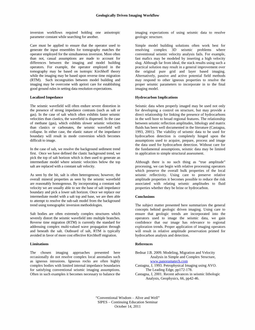
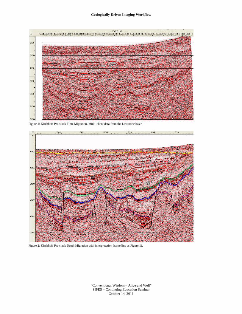
Developing a refined model based upon an inter-play of layers, guiding horizons and local grid based solutions is a very interpretative process. Many false starts may be necessary before a proper solution is found which satisfies regional and sub-regional geologic trends. Often the seismic data itself will dictate the spatial and temporal limitations imposed by the field acquisition/recording operator. The model complexity should be deliberately controlled by the choice of imaging operator (time or depth). Care must be given to considering whether the choice of imaging operator is able to handle the level of detail imposed by the geologic interpretation. The level of detail in the geology should directly correlate to the geophysical assumptions imposed by the choice of imaging algorithm. Time versus Depth There is a long history of mathematics for modeling the propagation of seismic wavefields through the Earth. Time and depth processing or imaging operators come in a wide array of permutations depending on the theory used to model the seismic data. Under simple acoustic assumptions, time migration operators are based upon smoothly varying rms velocities whereas depth imaging requires the use of interval velocities which may impart significant detail in geologic structure. Fortunately linear relationships may be assumed for relating rms and interval velocities such that the geologic information generated in time may then be used as a guide for the depth imaging workflow. In our staged model building approach we leverage the value of each successively complex migration algorithm to extract the most value from imaging. As we improve the operator accuracy so does our ability to resolve finer features of the sediment structure. Initial focus is placed on estimating a simple background trend based upon vertical variations in velocity structure as a function of lateral position. Our understanding of the geology is tied to our understanding of the imaging as we transition from simple isotropic time migration to more complicated pre-stack depth imaging. For example, we often expect complex structure seen in a Kirchhoff pre-stack time product to improve and focus when the imaging operator is upgraded to Kirchhoff pre-stack depth (Figures 1 and 2). Anisotropy Further enhancement of the depth model might be improved by incorporating corrections for lateral and vertical variations in velocity related to spatial changes related to structure or stratigraphy. Such details in lithology may be incorporated into the appropriate seismic velocity model through simultaneous inversion of anisotropic properties. Older

Geologically Driven Imaging Workflow

“Conventional Wisdom – Alive and Well” SIPES – Continuing Education Seminar

October 14, 2011

inversion workflows required holding one anisotropic parameter constant while searching for another. Care must be applied to ensure that the operator used to generate the input ensembles for tomography matches the operator employed for the simultaneous inversion. More often than not, casual assumptions are made to account for differences between the imaging and model building operators. For example, the operator employed in the tomography may be based on isotropic Kirchhoff theory while the imaging may be based upon reverse time migration (RTM). Such incongruities between model building and imaging may be overcome with apriori care for establishing good ground rules in setting data resolution expectations. Localized Impedance The seismic wavefield will often endure severe distortion in the presence of strong impedance contrasts (such as salt or gas). In the case of salt which often exhibits faster seismic velocities than clastics, the wavefield is dispersed. In the case of methane (gas), which exhibits slower seismic velocities than clastics or carbonates, the seismic wavefield will collapse. In either case, the elastic nature of the impedance boundary will result in mode conversion which becomes difficult to image. In the case of salt, we resolve the background sediment trend first. Once we have defined the clastic background trend, we pick the top of salt horizon which is then used to generate an intermediate model where seismic velocities below the top salt are replaced with a constant salt velocity. As seen by the bit, salt is often heterogenous; however, the overall mineral properties as seen by the seismic wavefield are reasonably homogenous. By incorporating a constant salt velocity we are usually able to see the base of salt impedance boundary and pick a lower salt horizon. Once we replace our intermediate model with a salt top and base, we are then able to attempt to resolve the sub-salt model from the background trend using tomographic inversion methodologies. Salt bodies are often extremely complex structures which severely distort the seismic wavefield into multiple branches. Reverse time migration (RTM) is currently the standard for addressing complex multi-valued wave propagation through and beneath the salt. Outboard of salt, RTM is typically avoided in favor of more cost effective Kirchhoff migration. Limitations The chosen imaging approaches presented here occasionally do not resolve complex local anomalies such as igneous intrusions. Igneous rocks are often highly complex bodies with limited internal impedance boundaries for satisfying conventional seismic imaging assumptions. Often in such examples it becomes necessary to balance the

imaging expectations of using seismic data to resolve geologic structure. Simple model building solutions often work best for resolving complex 3D seismic problems where conventional seismic velocity analysis fails. For example, fast mafics may be modeled by inserting a high velocity slug. Although far from ideal, the stack results using such a practical solution may result in a general improvement over the original pure grid and layer based imaging. Alternatively, passive and active potential field methods may respond to other igneous properties to resolve the proper seismic parameters to incorporate in to the final imaging model. Hydrocarbon Implications Seismic data when properly imaged may be used not only for developing a control on structure, but may provide a direct relationship for linking the presence of hydrocarbons in the well bore to broad regional features. The relationship between seismic reflection amplitudes, lithology and matrix fluids has been well documented in the literature (Castagna, 1993, 2001). The viability of seismic data to be used for hydrocarbon detection is completely hinged upon the assumptions used to acquire, prepare, process and image the data used for hydrocarbon detection. Without care for the fundamental assumptions, seismic data may be limited in application to simple structural assessment. Although there is no such thing as “true amplitude” processing, we can begin with relative processing operators which preserve the overall bulk properties of the local seismic reflectivity. Using care to preserve relative amplitude properties it becomes possible to reduce the risk associated with relating seismic amplitudes to fluid properties whether they be brine or hydrocarbon. Conclusions The subject matter presented here summarizes the general concepts behind geologic driven imaging. Using care to ensure that geologic trends are incorporated into the operators used to image the seismic data, we gain confidence that our image has relevance to regional exploration trends. Proper application of imaging operators will result in relative amplitude preservation primed for hydrocarbon analysis and detection. References Bednar J.B. 2009. Modeling, Migration and Velocity Analysis in Simple and Complex Structure, www.panoramatech.com Castagna, J, 1993. Petrophysical Imaging using AVO. The Leading Edge, pp172-178. Castagna, J, 2001. Recent advances in seismic lithologic Analysis, Geophysics, 66, pp42-46.

Geologically Driven Imaging Workflow

“Conventional Wisdom – Alive and Well” SIPES – Continuing Education Seminar

October 14, 2011

Figure 1: Kirchhoff Pre-stack Time Migration. Multi-client data from the Levantine basin

Figure 2: Kirchhoff Pre-stack Depth Migration with interpretation (same line as Figure 1).