Embed Size (px)
Citation preview

Journal of Complexity 28 (2012) 320–345
Contents lists available at SciVerse ScienceDirect
Journal of Complexity
journal homepage: www.elsevier.com/locate/jco
A geometric algorithm for winding number computationwith complexity analysisJuan-Luis García Zapata a,∗, Juan Carlos Díaz Martín b
a Departamento de Matemáticas, Escuela Politécnica, Universidad de Extremadura, Avda. de la Universidad s/n 10071, Cáceres, Spainb Departamento de Tecnología de los Computadores, Escuela Politénica, Universidad de Extremadura, Avda. de la Universidad s/n10071, Cáceres, Spain
a r t i c l e i n f o
Article history:Received 13 January 2011Accepted 26 January 2012Available online 21 February 2012
Keywords:Winding numberContour integrationArgument principleRoot finding
a b s t r a c t
Many methods to compute the winding number of plane curveshave been proposed, often with the aim of counting the numberof roots of polynomials (or, more generally, zeros of analyticfunctions) inside some region by using the principle of argument.In this paper we propose another method, which are not basedon numerical integration, but on discrete geometry. We giveconditions that ensure its correct behavior, and a complexity boundbased on the distance of the curve to singular cases. Besides, weprovide a modification of the algorithm that detects the proximityto a singular case of the curve. If this proximity is such that thenumber of operations required grows over certain threshold, set bythe user, the modified algorithm returns without winding numbercomputation, but with information about the distance to singularcase. When the method is applied to polynomials, this informationrefers to the localization of the roots placed near the curve.
© 2012 Elsevier Inc. All rights reserved.
1. Introduction: winding number and root finding
The winding number, or index, of a plane closed curve ∆ is the number of twists that it makesaround the origin. Its value can be computed using Cauchy integral formula of Complex Analysis as:
Ind(∆) =1
2π i
∆
dzz
.
∗ Corresponding author.E-mail addresses: [email protected] (J.-L. García Zapata), [email protected] (J.C. Díaz Martín).
0885-064X/$ – see front matter© 2012 Elsevier Inc. All rights reserved.doi:10.1016/j.jco.2012.02.001

J.-L. García Zapata, J.C. Díaz Martín / Journal of Complexity 28 (2012) 320–345 321
The main motivation for the study of winding number computation has been its use in severalroot-finding algorithms. They are based on the fact that the number of roots of a polynomial f insidethe curve Γ matches with the winding number of ∆ = f (Γ ). We can divide the plane region insideΓ (if it contains some root) in smaller regions. The winding number of its borders is computed and,recursively, these regions are divided in sub regions again if they contain some root, until the desiredprecision is reached. A similar procedure can be used to find the zeros of analytic functions [13].
The most used methods of root finding have been traditionally the iterative ones, like Newton,Jenkins–Traub or eigenvalue based, for example. The methods of this type converge rapidly, formost polynomials of moderate degree (less than about 50 [15]). Even for these degrees, the iterativemethods are inadequate for certain classes of polynomials (as those with clusters or multiple roots,depending on the method), or for specific polynomials that show ill-conditioning (like Wilkinsonexample). To cope with these issues, it is necessary to apply heuristic rules in case of difficulties(to choose another initial approximations, or change the method applied, or use high precisionarithmetic).
The methods based on geometrical relations (like winding number and others) are instead validfor all polynomials equally. Besides, this uniformity allows an analysis of the complexity for suchmethods. The theoretical studies of complexity have been a driving force in the development ofgeometric methods. In addition, practical applications need methods that allow to focus the rootfinding on a specified complex plane region [17]. This restriction produces a computational savingwith respect to iterative methods, which do not allow it. Geometric methods different from thewinding number are for example the inclusion test of Weyl [9,21], or the process of Graeffe [2].
Several root-finding algorithms that compute the winding number using numerical computationof the Cauchy integral have been proposed [13,19]. A different approach can be found in [20] or [5],using Sturm successions to find the crossings of the curve ∆ by positive abscissa axis. These methodsare valid for specific shapes of contour Γ (circular in Suzuki, rectangular in Wilf and Collins), andshow several troubles (the need of arbitrary-precision arithmetic [10] in the numerical integrationmethods, and a symbolic algebra package in themethods using Sturm successions).We follow anotherapproach, which can be traced to Henrici [9], using geometrical facts about a sample of the pointsof ∆. Our method is applicable to generic curves using standard IEEE 754 double precision. It hasbeen implemented and compared against several root finders, with good results [8]. We applied it topolynomials of high degree arising in signal processing. Others applications demanding high degreeroot finding are computer-algebra systems [15], robotics (the inverse cinematic problem) [17] orantenna theory [14].
Methods derived from Henrici have been used in recursive root-finding algorithms, either forpractical applications [18,8] or for theoretical studies of root-finding complexity [16,15]. In [22]or [12] we can find precise statements about the conditions in which we can use winding numberin root-finding algorithms, and suggestions to manage near-to-singular cases. But the study of theircomplexity, essential to compare these algorithms against traditional root finders, is unattended. Thispaper aims to fill this gap.
For this purpose, we will show that the distance of the curve ∆ from the origin is a measure ofthe cost of its winding number computation. We call this distance the value of singularity of ∆. Inparticular, in the use of the winding number to find roots of a polynomial f , the value of singularityof ∆ = f (Γ ) is equivalent to the distance from the roots of f to Γ . The mentioned works wereaware of the influence of this distance in the computational cost of the root finding, but they lacka precise expression of this dependence. Besides, we give cost bounds for the treatment of near-to-singular cases, which arisewhen using thewinding number algorithm recursively inside a root findingalgorithm.
The value of singularity of ∆ is the main factor in the cost of the algorithm. The reciprocal of thisvalue can be compared with the condition number of a matrix in linear numerical analysis. Both area measure of the ill-conditioning of the input data: the cost of a matrix inversion with a predefinedprecision, for example, grows proportionally to the condition number of thematrix. Similarly, the costof a winding number computation grows with the reciprocal of the value of singularity.
Beyond its theoretical interest, it is necessary a study of the value of singularity for the useof winding number in root-finding applications, because singular contours arise in the recursive
322 J.-L. García Zapata, J.C. Díaz Martín / Journal of Complexity 28 (2012) 320–345
subdivision of the plane region. In the treatment of these cases, we replace the singular contour byanother curve, closely situated, with higher value of singularity. This detour technique is similar toone proposed in [22], but armed with our results about the value of singularity we can apply it withina recursive procedure, hence we can handle curves with arbitrary singularity, as appears in [8].
About the structure of the paper, Section 2 below exposes the winding number algorithm, calledinsertionprocedure (IP). Section 3 studies its computational cost, depending on the value of singularityof the curve, if it is uniformly parameterized, and Section 4 develops an analogous study for the moregeneral Lipschitzian curves. Section 5 states a condition for the accuracy of the algorithm to count thetwists of any size around the origin (insertion procedure valid for any array, IPA). Section 6 introducesa control, intended for the application of the algorithm to curves of arbitrary value of singularity(insertion procedurewith control of singularity, IPS). The summarizing Section 7 includes suggestionsof future work.
2. Definitions and insertion procedure
Let us consider closed curves defined parametrically, that is, as mappings from a real interval tothe complex plane ∆ : [a, b] → C with ∆(a) = ∆(b). As usual in the study of parameterized curves,two curves ∆1 : [a, b] → C and ∆2 : [c, d] → C with the same image Im(∆1) = Im(∆2) canbe viewed as two parameterizations of a subset of C. Remember that a curve ∆ : [a, b] → C isuniformly parameterized if the arc length equals the length of the interval of the parameter values,that is, for each x, y ∈ [a, b], |y − x| =
yx d∆(t). Every piecewise differentiable curve can be
parameterized in a uniform way [11]. That is, for any curve ∆ : [a, b] → C there is another curve∆u
: [0, arclength(∆)] → C with Im(∆) = Im(∆u) and ∆u uniformly parameterized.We also consider Lipschitzian curves (that is, verifying that there exist a constant L with |∆(y) −
∆(x)| ≤ L|y − x| for each x, y ∈ [a, b], see [11]). The uniform parameterized curves are a particularcase of Lipschitzian ones, with L = 1.
The winding number, or index, Ind(∆) of a curve ∆ : [a, b] → C, is an integer number that countsthe complete rotations of the curve around the point (0, 0) in counterclockwise sense. See Fig. 1.
As a particular case of the Cauchy formula of Complex Analysis, the winding number is equal tothis line integral:
Ind(∆) =1
2π i
∆
1w
dw.
The winding number is applied in the principle of argument [9]. It states that the number of zeros(counted with multiplicity) of an analytic function f : C → C, w = f (z), inside a region with borderdefined by the curve Γ , is equal to the winding number of the curve ∆ = f (Γ ) (see Fig. 2). Theprinciple of argument can be viewed as a bi-dimensional analogy of Bolzano’s theorem, and it is in thebase of the recursive methods to find the zeros of holomorphic functions and, in particular, roots ofpolynomials.
It should be noted that the winding number of the curve ∆ is not defined if ∆ crosses over theorigin (0, 0) because the integral
∆
1w
dw does not exist. In that case, ∆ is called a singular curve. If∆ = f (Γ ), this is equivalent to that Γ crosses over a zero of f . For a value ε ≥ 0, we say that a curveis ε-singular if its minimum distance to the origin is ε. The 0-singular curves are the curves previouslycalled singular for the index integral. The Cauchy formula is not applicable to 0-singular curves.
As commented in the introduction, we take the approach of Henrici [9] as an alternative tonumerical integration of the above formula. Hence, we work with polygonal approximations of thecurve ∆, that is, discrete sets of complex points disposed in certain order: for an array of parametervalues si ∈ [a, b], (a = s0, . . . , sn = b) with s0 < s1 < · · · < sn, the polygonal approximation is∆n = (∆(s0), . . . , ∆(sn)). Fig. 3 shows a curve with a polygonal approximation.
For an array S = (s0, . . . , sn) of increasing values, si < si+1, i = 0, . . . , n − 1, we call its maxstep|S| to the maximum difference between consecutive values, that is: |S| = max0≤i≤n−1(si+1 − si).
The complex plane is divided in angular sectors, of angle π4 . There are eight such sectors, called
C0, C1, C2, . . . , C7, each one the half of a quadrant. To be precise, each border between adjacent sectors,Cx and Cx+1, is included in Cx+1 for x = 0, . . . , 6, and the border between C7 and C0 is included in C0.

J.-L. García Zapata, J.C. Díaz Martín / Journal of Complexity 28 (2012) 320–345 323
Fig. 1. The winding numbers of the curves ∆1 and ∆2 are Ind(∆1) = 1 and Ind(∆2) = 2.
Fig. 2. The number of roots of the polynomial f (z) = z3 + 1 inside Γ1 and Γ2 equals the winding numbers of ∆1 = f (Γ1) and∆2 = f (Γ2), respectively.
Fig. 3. The curve ∆ is approximated by polygonal ∆18 with a resolution of 18 points.
We say that two points p, q of the curve ∆ are connected if they are placed in two adjacent sectorsor the same one, that is, if p, q ∈ Cx ∪ Cx+1 for some x. Equivalently, if p ∈ Cx and q ∈ Cy implies thaty = x ± 1 (or y = x). As the sectors C7 and C0 are adjacent, the equalities must be understood as anarithmetic congruence modulo 8.

324 J.-L. García Zapata, J.C. Díaz Martín / Journal of Complexity 28 (2012) 320–345
Fig. 4. Curve segments with number N of crossed borders.
Let us consider the borders delimiting sectors C0, . . . , C7. For each curve segment ∆([si, si+1]) wesay that it crosses N borders if the parameter interval contains at most N values fj, j = 1, . . . ,N , withsi ≤ f1 < f2 < · · · < fN ≤ si+1, whose image points∆(fj) belong to some border. For example in Fig. 4there are several segments with the number of borders that they cross.
Let us suppose that the curve ∆ has a defined index, that is, it does not cross the origin. Then it issure that there is an array (t0, t1, . . . , tm) of values of the parameter t ∈ [a, b], a = t0 < t1 < · · · <tm = bwhose images by the mapping ∆ are connected, as shown in Fig. 5.
We say that a polygon of vertices ∆(ti), i = 0, 1, . . . ,m verifies the property of connection if everypair of consecutive points ∆(ti) and ∆(ti+1) are connected. If we get for any method an array ofpoints (∆(t0), ∆(t1), . . . , ∆(tm)) defining a polygon ∆m that verifies the property of connection, itsindex Ind(∆m) can be calculated as the number of points ∆(ti) in C7 followed by a point ∆(ti+1) inC0. The occurrence of a sector C0 followed by C7 must be counted negatively. That is, Ind(∆m) =
#(crossings C7 to C0) − #(crossings C0 to C7).The method to find the parameter values (t0, t1, . . . , tm) was left unspecified by Henrici, as well
as the conditions under which the index of the approximating polygon ∆m coincides with that of theoriginal curve∆. Ying and Katz [22] proposed such amethod, at a reasonable computational cost. Theyconstruct such array starting from some initial array of parameter values (a = s0, . . . , sn = b) of thecurve ∆, whose images not necessarily verify the property of connection, i.e., that perhaps, for somei, the images of si and si+1 are not connected. The array of images ∆(si) is scanned from the beginnings0, until a pair (si, si+1) is found such that its images∆(si) ∈ Cx and∆(si+1) ∈ Cy are not connected. Inthis situation an interpolation value si+si+1
2 is inserted in parameter array (s0, . . . , sn) between si andsi+1. Then the resulting array (s′0, . . . , s
′
n+1) is scanned again for another pair (s′j, s′
j+1) whose imagesare not connected and a middle point is inserted as described. Iterating this process, finally an arrayT = (t0, . . . , tm), m ≥ n, is obtained whose images verify the property of connection. This procedureis defined in Fig. 6.

J.-L. García Zapata, J.C. Díaz Martín / Journal of Complexity 28 (2012) 320–345 325
Fig. 5. The images of the successive values ti , ti+1 are connected.
Fig. 6. Insertion procedure (Ying and Katz).
The insertion process scans the array from left to right, in such a way that the points needed toconnect si and si+1 are inserted before those between si+1 and si+2.
This procedure of interpolation-point insertion has two details that make difficult its effectiveapplication in index calculation. In first place, it does not end in a finite number of steps in certaincases. We discuss this in the Sections 3 and 4. In second place, Ind(∆m) coincides with the index of ∆only under certain assumptions. The Section 5 deals with this issue of the coincidence of Ind(∆m)

326 J.-L. García Zapata, J.C. Díaz Martín / Journal of Complexity 28 (2012) 320–345
and Ind(∆). The analysis of the insertion procedure, and its modification bringing to a finite anddemonstrable algorithm for winding number calculation, is the main contribution of this work.
3. Complexity of the insertion procedure for uniformly parameterized curves
If the curve ∆ crosses over the origin (that is, ∆ is a singular curve) the insertion procedure cannotreach an end, because there is not any array of points with the property of connection. Besides, if thecurve is placed very close to the origin, the number of insertions can grow to a high value. The purposeof this section is to give a precise statement of this fact, in Theorem 1 below.
Suppose that we apply the insertion procedure with initial array S(0)= (s0, . . . , sn). Let us focus
on an interval [si, si+1]whose image, the curve segment∆([si, si+1]), has its end points not connected(see Fig. 7). We call Cx the sector containing ∆(si), and pk the k-th point resulting from an insertion ofthe procedure between ∆(si) and ∆(si+1), k = 1, 2, . . .. Also we call uk the parameter value such thatpk = ∆(uk), so S(k)
= (s0, . . . , si, . . . , uk, . . . , si+1, . . . , sn).Note that the insertions uk in the parameter array are not necessarily performed in increasing
order, that is, not necessarily uk < uk+1. To manage this unpredictability of the insertion point, letus call the point array ∆(S(k)) = (. . . , ∆(si), . . . , pk, . . . , ∆(si+1), . . .), and let us call q1 and q2 thefirst not connected points found in this array in the left-to-right scanning of the insertion procedure:∆(S(k)) = (. . . , ∆(si), . . . , q1, q2, . . . , ∆(si+1), . . .). Despite this expression, note that it is possiblethat q1 = ∆(si) or q2 = ∆(si+1), or that q1 or q2 equals to pk. Suppose that no point of the array∆(S(k)) between ∆(si) and ∆(si+1) belongs to Cx−1 neither to Cx+1, the adjacent sectors to the onecontaining∆(si). Then we have that q1 ∈ Cx and q2 ∈ (Cx−1 ∪Cx ∪Cx+1)
c . This is because the insertionprocess scans the array in increasing order of the parameter value, and then the points of the segment(∆(si), . . . , q1) of ∆(S(k)) must all belong to Cx (as they are connected, ∆(si) ∈ Cx, and there are nopoints in Cx−1 neither in Cx+1). And hence the non adjacent point q2 must belong to a non adjacentsector, that is, q2 ∈ (Cx−1 ∪ Cx ∪ Cx+1)
c .The following proposition formalizes this reasoning, calling Ik the curve segment joining pk with
the previous point in array, and I ′k the curve segment joining pk with the subsequent point. Wedefine I0 = I ′0 = ∆([si, si+1]). For example, as p1 = ∆(u1), we have that I1 = ∆([si, u1]) andI ′1 = ∆([u1, si+1]) (see Fig. 8).
As notation issue, in the following propositions the set of points {p1, p2, . . . , pk−1} should beviewed as {p1, p2} when k = 3, {p1} when k = 2 and the void set when k = 1.
Proposition 1. Suppose that ∆(si) and ∆(si+1) are not connected. For k = 1, 2, . . . , if the sectors Cx−1and Cx+1 do not contain any point from p1, p2, . . . , pk−1, then it is verified:
(a) If pk belongs to Ck, then I ′k has one endpoint in Cx and the other one in (Cx−1 ∪ Cx ∪ Cx+1)c .
(b) If pk belongs to (Cx−1∪Cx∪Cx+1)c , then Ik has one endpoint in Cx and the other one in (Cx−1∪Cx∪Cx+1)
c .
Proof. As the insertion points p1, p2, . . . , pk−1 are not contained in Cx−1 neither in Cx+1, by the abovereasoning the points q1 = ∆(v1) and q2 = ∆(v2) first found by the left–right scanning of the insertionproceduremust verify q1 ∈ Cx and q2 ∈ (Cx−1∪Cx∪Cx+1)
c . Therefore, if pk ∈ Cx, then I ′k = ∆([uk, v2])verifies the claim of (a). Likewise if pk ∈ (Cx−1 ∪ Cx ∪ Cx+1)
c , Ik = ∆([v1, uk]) verifies the claimof (b). �
To proceed with the argumentation, we need a further hypothesis about ∆. In this section wesuppose that ∆ : [a, b] → C is uniformly parameterized (that is, for each x, y ∈ [a, b], |y − x| = yx d∆(t)).We callM the arc length of the segment∆([si, si+1]). If∆ is uniformly parameterized, we have [11]
thatM = (si+1 − si).
Proposition 2. If k is such that the sectors Cx−1 and Cx+1 do not contain any point fromp1, p2, . . . , pk−1, pk, then pk+1 is the midpoint of either Ik or I ′K , the one with its endpoints not connected.Besides, if ∆ is uniformly parameterized, then for j = 1, 2, . . . , k+1, arclength(Ij) = arclength(I ′j ) =
M2j.
In particular, arclength(Ik) = arclength(I ′k) =M2k.

J.-L. García Zapata, J.C. Díaz Martín / Journal of Complexity 28 (2012) 320–345 327
Fig. 7. The parameter array produced by insertion procedure in this curve is S(4)= (. . . , si, u2, u4, u3, u1, si+1, . . .). The next
insertion point p5 goes between p2 and p4 .
Fig. 8. The points ∆(si) and ∆(si+1) and the intervals Ik and I ′k are outlined.
Proof. By induction: for k = 0, p1 is the midpoint of I0 = I ′0 = ∆([si, si+1]) because of the uniformparameterization. For general k, the induction hypothesis is that pk is the midpoint of Ik−1 or I ′k−1. Thearray after this k-th insertion outcomes (. . . , ∆(si), . . . , e1, pk, e2, . . . , ∆(si+1), . . .), being e1, e2 thenot connected endpoints of one of the two segments Ik−1 or I ′k−1. Note that as pk is not in Cx−1 neitherin Cx+1, then must be pk ∈ Cx or pk ∈ (Cx−1 ∪ Cx ∪ Cx+1)
c , and by Proposition 1 the endpoints of eitherIk (that are e1, pk) or I ′k (that are pk, e2) are not connected. The next insertion point pk+1 is producedby the procedure after finding two points q1 and q2 not connected. By the left–right scanning of thearray, we must conclude that these points are either q1 = e1 and q2 = pk, or q1 = pk and q2 = e2.That is, pk+1 is the midpoint of Ik or I ′k.
For the claim about the lengths, note that arclength(I0) = arclength(I ′0) = M , and that, forj = 1, 2, . . . , k + 1, pj divides either Ij or I ′j in two halves, Ij+1 and I ′j+1. Therefore arclength(Ij+1) =
arclength(I ′j+1), and arclength(Ij+1) =arclength(Ij)
2 , and by induction we derive the expression for thearc length. �

328 J.-L. García Zapata, J.C. Díaz Martín / Journal of Complexity 28 (2012) 320–345
Remember that a curve is ε-singular if its minimum distance to the origin is ε. We have that:
Proposition 3. The arc length of a segment of an ε-singular curve with its endpoints not connected isstrictly greater than π
4 ε.
Proof. This can be viewed considering a circumference of radius ε, for instance the one depicted witha dash line in Fig. 8. It is the curvewithminimal arc length between the ε-singular ones. And its pointsin different non adjacent sectors has an angle difference with a lower bound of π
4 , corresponding toan arc length of π
4 ε. �
With the decrement of the arclength of the intervals in the conditions of Proposition 2, and theconcept of ε-singularity, we advance in the proof of the finiteness of the insertion process betweensi and si+1. We can foresee that the number of insertions should be bound by a formula involvinglogarithms, because each insertion divides by two the difference between two consecutive parametersof the array. Proposition 4 gives us the concrete bound of ⌈lg2(
4Mπε
)⌉ for the number of iterations untilan insertion point is connected to ∆(si).
Proposition 4. Suppose that ∆ is uniformly parameterized and ε-singular. If ∆(si) and ∆(si+1) arenot connected, being Cx the sector containing ∆(si), then there is an insertion point pK verifying pK ∈
Cx−1 ∪ Cx+1 with K ≤ ⌈lg2(4Mπε
)⌉.
Proof. Webuild a bound of the number of iterations of the insertion procedure until an insertion pointpertains to Cx−1 ∪ Cx+1. Let us define k0 as the integer verifying M
2k0≤
π4 ε < M
2k0−1 . This is equivalentto 4M
πε≤ 2k0 < 2 4M
πε, that is lg2(
4Mπε
) ≤ k0 < lg2(4Mπε
) + 1, therefore k0 = ⌈lg2(4Mπε
)⌉. Note that byProposition 3 the arc length of ∆([si, si+1]), M , verifies M > πε
4 , that is 4Mπε
> 1, hence lg2(4Mπε
) > 0and ⌈lg2(
4Mπε
)⌉ ≥ 1. Then k0 ≥ 1.If for some K with K < k0 the insertion point pK verifies pK ∈ Cx−1 ∪ Cx+1, then the conclusion of
the proposition is verified, because K < k0 = ⌈lg2(4Mπε
)⌉. If, on the contrary, all the insertion pointspK with K < k0 verify pK ∈ Cx−1 ∪ Cx+1 (or equivalently, the sectors Cx−1 and Cx+1 do not contain anypoint from p1, p2, . . . , pk0−1) we are in the hypothesis of Proposition 1 (with k = k0). If we suppose,seeking a contradiction, that pk0 ∈ Cx−1∪Cx+1 (that is, pk0 ∈ Cx or pk0 ∈ (Cx−1∪Cx∪Cx+1)
c), then eitherIk0 or I
′
k0has its endpoints not connected. Besides, we have that arclength(Ik0) =
M2k0
by Proposition 2,and M
2k0≤
π4 ε by definition of k0. And it is not possible that arclength(Ik0) = arclength(I ′k0) ≤
π4 ε
with its endpoints not connected, because this contradicts Proposition 3. We must conclude thatpk0 ∈ Cx−1 ∪ Cx+1. �
Note that being pK the first insertion point with pK ∈ Cx−1 ∪ Cx+1, the points in the segment(∆(si), . . . , q1) of the array S = (. . . , ∆(si), . . . , q1, pK , q2, . . . , ∆(si+1), . . .) belong to Cx. This isbecause the insertion procedure scans the array from left to right, and then it is not possible that oneof these points (∆(si), . . . , q1) belongs to (Cx−1∪Cx∪Cx+1)
c , since in such case theK -th insertion pointshould be inserted in a place preceding q1. Also it is not possible that some of these points belong toCx−1∪Cx+1, because pK is the first inserted point with this property. Then the points of (∆(si), . . . , q1)must belong to Cx.
Using Proposition 4 we can find a bound to the number of insertion points required to connect∆(si) and ∆(si+1). Remember that ∆([si, si+1]) crosses N borders between sectors if the parameterinterval contains at most N values fj, j = 1, . . . ,N , with si ≤ f1 < f2 < · · · < fN ≤ si+1, whose imagepoints ∆(fj) belong to some border.
Note that if ∆([si, si+1]) crosses N = 0 borders, the number of insertion points required in thissegment is zero because ∆(si) and ∆(si+1) are in the same sector. Likewise, if N = 1, then ∆(si) and∆(si+1) are connected, and no insertion point is required. In case of greater number of crosses N , thefollowing claim is verified:
Lemma 1. Suppose that ∆ is uniformly parameterized and ε-singular, that ∆(si) and ∆(si+1) are notconnected, and that ∆([si, si+1]) crosses N borders. For N ≥ 2, the number of insertion points between∆(si) and ∆(si+1) is bounded by (N − 1)⌈lg2(
4Mπε
)⌉.

J.-L. García Zapata, J.C. Díaz Martín / Journal of Complexity 28 (2012) 320–345 329
Fig. 9. The curve segment between ∆(si) and ∆(si+1) has an arc length of M , and ∆([si, si+1]) crosses 4 borders.
Proof. We prove that assert by induction on N .Suppose firstly that N = 2; as ∆(si) and ∆(si+1) are not connected, the points of ∆([si, si+1]) are
contained in three sectors. Cx is the sector containing ∆(si), then there are two possible cases: either∆(si) ∈ Cx, ∆(si+1) ∈ Cx+2 and ∆([si, si+1]) ⊂ Cx ∪ Cx+1 ∪ Cx+2 (counterclockwise), or ∆(si) ∈ Cx,∆(si+1) ∈ Cx−2 and ∆([si, si+1]) ⊂ Cx ∪ Cx−1 ∪ Cx−2 (clockwise). Fig. 8 depicts the first case. ByProposition 4, in less than ⌈lg2(
4Mπε
)⌉ iterations the insertion procedure puts a point pK in Cx−1 ∪ Cx+1.With this insertion the array (∆(si), . . . , pK , . . . , ∆(si+1)) verifies the property of connection and theprocedure ends (between ∆(si) and ∆(si+1)).
This reasoning on N = 2 is the base case of the induction proving the lemma. For the inductivestep, suppose now that the curve segment ∆([si, si+1]), of length M , crosses N borders, N > 2.The hypothesis of induction, that we suppose proved, is that any curve segment crossing N − 1borders requires at most (N − 2)⌈lg2(
4M ′
πε)⌉ insertions points, being M ′ its length. We shall prove
that ∆([si, si+1]) requires at most (N − 1)⌈lg2(4Mπε
)⌉ insertion points, by dividing this segment in twosections, a first one that goes from ∆(si) to a point in Cx−1 or Cx+1, and a second one that goes fromthis point to ∆(si+1).
By Proposition 4, we have that for certain K ≤ ⌈lg2(4Mπε
)⌉, the point pK = ∆(uK ) is in a sectorwhichis adjacent to ∆(si), either Cx−1 or Cx+1. Besides, by the note following the proof of Proposition 4, thepoints in the segment (∆(si), . . . , q1) of the array (. . . , ∆(si), . . . , q1, pK , q2, . . . , ∆(si+1), . . .) belongto Cx. Fig. 9 shows an example where K = 3 and pK ∈ Cx+1.
We divide the segment ∆([si, si+1]) in two subsegments, ∆([si, uK ]) and ∆([uK , si+1]). Note that∆([si, uK ]) crosses at least one border (that one between Cx and Cx−1 or Cx+1), but not necessarilyonly one, as we can see for example in the positions of Fig. 10. Besides, after the K -th iteration theinsertion process does not insert points in ∆([si, uK ]), because all the points of the array in thissegment (∆(si), . . . , q1, pK ) belong to Cx except pK that belong to Cx−1 or Cx+1.
Let us call α the number of borders crossed by ∆([si, uK ]). The rest of the original curve segment,∆([uK , si+1]), crosses N − α borders, with α ≥ 1. Let us consider ∆([uK , si+1]) as a curve that crossesN − 1 borders or less. Remember that the hypothesis of induction is that any curve segment crossingN − 1 borders requires at most (N − 2)⌈lg2(
4M ′
πε)⌉ insertions points, being M ′ its length. Therefore
∆([uK , si+1]) requires at most (N − 2)⌈lg2(4M ′
πε)⌉ insertions, being the arc lengthM ′
= (si+1 − uK ). Toconclude, we have that with K insertions (being K ≤ ⌈lg2(
4Mπε
)⌉), the segment ∆([si, si+1]) gives riseto a subsegment∆([uK , si+1]), that requires atmost (N−2)⌈lg2(
4M ′
πε)⌉ insertions. In total less or equal
than ⌈lg2(4Mπε
)⌉+(N−2)⌈lg2(4M ′
πε)⌉ insertions. AsM ′ < M , this is lesser or equal than (N−1)⌈lg2(
4Mπε
)⌉,that is the asserted claim. �

330 J.-L. García Zapata, J.C. Díaz Martín / Journal of Complexity 28 (2012) 320–345
Fig. 10. The segment ∆([si, uK ]) crosses as least one border. q1 is the point previous to pK along the array.
Weobtain the theorem avoiding the dependence ofN in the above lemma, bounding themaximumnumber N of borders crossed by a segment of arc lengthM of an ε-singular curve.
Remember that for an array S = (s0, . . . , sn), its maxstep is |S| = max0≤i≤n−1(si+1 − si).
Theorem 1. If ∆ : [a, b] → C is ε-singularwith ε > 0, uniformly parameterized, the insertion procedurefor the curve∆with an initial array S(0)
= (s0, . . . , sn) of increasing values, with s0 = a, sn = b concludesin less than 4(b−a)
πε⌈lg2(
4|S(0)|
πε)⌉ insertions.
Proof. Let us consider a circular curve placed at constant distance ε from the origin. It has a distancealong the curve between points in different borders of πε
4 . Any other curve ε-singular has a distancebetween points in different borders greater or equal than that value. Hence, among the curves of arclength M , the circular curve has the maximum number of borders crossed. To compute this number,Nmax, let we call fj, j = 1, . . . ,Nmax, the parameter values corresponding to points ∆(fj) on a border, inincreasing order, fj < fj+1. Two consecutive points ∆(fj), ∆(fj+1) are at a distance along the curve ofπε4 , and by uniform parameterization, (fj+1 − fj) =
πε4 . In general, to calculate the number x of points
at a distance d inside an interval of length m, consider that with x points equally spaced at distance dwe cover a length of (x− 1)d. Then we have that (x− 1)d ≤ m < xd, that is x = ⌊
md ⌋ + 1. In our case,
the number Nmax of parameter values fj at a distance of πε4 is ⌊
Mπε4
⌋ + 1 = ⌊4Mπε
⌋ + 1. Then the numberof borders crossed by any curve should be lesser or equal than this value. In particular, being N thenumber of borders crossed by ∆([si, si+1]), N ≤ Nmax = ⌊
4Mπε
⌋ + 1, hence N − 1 ≤4Mπε
. Applying theprevious lemma, the maximum number of insertion points in ∆([si, si+1]) is bound by 4M
πε⌈lg2(
4Mπε
)⌉.We have derived a bound 4M
πε⌈lg2(
4Mπε
)⌉ for the number of insertion points required in ∆([si, si+1]).This is valid for each i, 0 ≤ i ≤ n − 1, being S(0)
= (s0, . . . , sn) the initial array,but the distance M between ∆(si) and ∆(si+1) can vary with i. In any case, this distance isequal to (si+1 − si) by the uniform parameterization. Summing up these maximums leads us ton−1
i=04(si+1−si)
πε⌈lg2(
4(si+1−si)πε
)⌉. Besides, (si+1 − si) are lesser or equal than |S(0)| by the definition of
maxstep. Then lg2(4(si+1−si)
πε) ≤ lg2(
4|S(0)|
πε) for i = 0, 1, 2, . . . , n−1, and the above summatory is lesser
or equal than (n−1
i=04(si+1−si)
πε)⌈lg2(
4|S(0)|
πε)⌉. This can be simplified because
n−1i=0 (si+1 − si) = (b− a),
and then the total of insertions is lesser or equal than 4(b−a)πε
⌈lg2(4|S(0)
|
πε)⌉. �
4. Complexity of the insertion procedure for Lipschitzian curves
We can generalize this theorem to handle ε-singular curves not necessarily uniformly parameter-ized. Note that the array resulting from the insertion procedure depends on the parameterization:

J.-L. García Zapata, J.C. Díaz Martín / Journal of Complexity 28 (2012) 320–345 331
i.e. two parameters ∆ and ∆′ with the same image curve in C can produce different insertion points.The above analysis of the complexity of the insertion procedure for uniformly parameterized curvescan be carried to themore general Lipschitzian parameterized curves (that is, verifying that there exista constant L with |∆(y) − ∆(x)| ≤ L|y − x| for each x, y ∈ [a, b]).
This relaxation of hypothesis is needed for our intended application [7], the computation ofthe index of curves ∆ = f (Γ ) with Γ surrounding an area of interest. The curve Γ is usuallydefined collating uniform parameterized segments, and this makes Γ uniformly parameterized.But its transformation ∆ is not uniformly parameterized for general polynomial f , although it isLipschitzian [11].
The number of insertion points in any Lipschitzian curve has the bound determined in theTheorem 2. The path followed to prove it is very similar to that of the Theorem 1.
For an initial array S(0)= (s0, . . . , sn) let us consider a curve segment ∆([si, si+1]). In this case
M = (si+1−si) is not the arc length of the segment. However, in a Lipschitzian curvewith constant L, itis verified that arclength(∆[s, t]) ≤ L(t−s) (see [11]). In particular arclength(∆[si, si+1]) ≤ (si+1−si).With this bound of the arc length we can prove Theorem 2 similarly to Theorem 1.
Let us call pk the k-th insertion point between∆(si) and∆(si+1), anduk its parameter, k = 1, 2, . . . ,like in the above demonstration. Also, for k = 1, 2, . . . , we call Ik the segment of the curve ∆ joiningpk with the previous point in the array, and I ′k the curve segment joining pk with the subsequent point.See Fig. 8.
The Proposition 1 of the previous section applies to curves of any kind of parameter. The nextproposition is specific to Lipschitzian curves, and is analogous to Proposition 2 of the previous section.
Proposition 5. Suppose that ∆ is Lipschitzian with constant L. If k is such that the sectors Cx−1 andCx+1 do not contain any point from p1, p2, . . . , pk−1, pk, then pk+1 has, as parameter, the mean of theparameters of the endpoints of either Ik or I ′k, that one with its endpoints not connected. Besides, forj = 1, 2, . . . , k + 1, arclength(Ij) ≤
LM2j
and arclength(I ′j ) ≤LM2j.
Proof. By induction: for k = 0, I0 = I ′0 = ∆([si, si+1]) and p1 has parameter u1 =si+si+1
2 , thatis the claim. For general k, the induction hypothesis is that pk = ∆(uk) with uk the mean of theparameters of the endpoints of Ik−1 or I ′k−1, that implies that the array after this insertion outcomes(. . . , ∆(si), . . . , e1, pk, e2, . . . , ∆(si+1), . . .), being e1, e2 the not connected endpoints of one of thetwo segments. The next insertion point pk+1 is produced by the procedure after finding two points q1and q2 not connected, and pk+1 has as parameter the mean of the parameters of these points. Notethat as pk is not in Cx−1 neither in Cx+1, then must be pk ∈ Cx or pk ∈ (Cx−1 ∪ Cx ∪ Cx+1)
c , and byProposition 1 the endpoints of either Ik (that are e1, pk) or I ′k (that are pk, e2) are not connected. As theprocedure scans the array from left to right, then the not connected points found are either q1 = e1and q2 = pk, or q1 = pk and q2 = e2. That is, pk+1 has as parameter the mean of the parameters of theendpoints of Ik or of I ′k.
Note that this reasoning is similar to that of Proposition 2 in the previous section, but now theinsertion point pk is not necessarily the midpoint of the curve segment between the not connectedpoints.
For the lengths, we have by induction that the difference between the parameters of the endpointsof Ij is M
2j, for j = 1, 2, . . . , k + 1. The same with I ′j . As commented above, in a Lipschitzian curve
with constant L, the arc length of a curve segment verifies arclength(∆[s, t]) ≤ L(t − s). Hencearclength(Ij) ≤ LM
2jand arclength(I ′j ) ≤ LM
2j. �
Finally, we prove:
Proposition 6. Suppose that ∆ is Lipschitzian of constant L and ε-singular. If ∆(si) and ∆(si+1) are notconnected, being Cx the sector containing ∆(si), then the first inserted point verifying pK ∈ Cx−1 ∪ Cx+1 issuch that K ≤ ⌈lg2(
4LMπε
)⌉.
Proof. Let us define k0 as the integer verifying LM2k0
≤π4 ε < LM
2k0−1 . We have that k0 = ⌈lg2(4LMπε
)⌉ ≥ 1.If the first insertion point pertaining to Cx−1∪Cx+1 is pK withK < k0, then the claimK ≤ ⌈lg2(
4LMπε
)⌉of the proposition is obvious. In contrary case, all the points p1, p2, . . . , pk0−1 are outside Cx−1 ∪ Cx+1,

332 J.-L. García Zapata, J.C. Díaz Martín / Journal of Complexity 28 (2012) 320–345
hence the insertion process reaches the k0-th iteration. We are in the hypothesis of Proposition 1(with k = k0), and if we suppose that pk0 ∈ Cx−1 ∪ Cx+1, hence either Ik0 or I ′k0 has its endpointsnot connected. Besides by Proposition 5, arclength(Ik0) = arclength(I ′k0) ≤
LM2k0
. By definition of k0 wehave that LM
2k0≤
π4 ε, so arclength(Ik0) = arclength(I ′k0) ≤
π4 ε. This however contradicts Proposition 3.
We must conclude that pk0 ∈ Cx−1 ∪ Cx+1. �
With this proposition, we can follow an argument similar to those of the previous section to showthat, if the curve segment ∆([si, si+1]) crosses N borders, the number of insertion points requiredcannot be higher than (N − 1)⌈lg2(
4LMπε
)⌉.
Lemma 2. Suppose that ∆ is Lipschitzian with constant L and ε-singular. For N ≥ 2, if ∆(si) and∆(si+1)are not connected, the number of insertion points is bounded by (N − 1)⌈lg2(
4LMπε
)⌉.
Proof. The proof of the lemma of the previous section can be repeated with the bound ⌈lg2(4LMπε
)⌉ ofProposition 6, instead of ⌈lg2(
4Mπε
)⌉, leading to the desired claim. �
Theorem 2. If ∆ : [a, b] → C is ε-singular with ε ≥ 0, and a Lipschitzian parameterization of constantL, then the insertion procedure for the curve ∆ with initial array S(0)
= (s0, . . . , sn), s0 = a, sn = b,concludes in less than 4L(b−a)
πε⌈lg2(
4L|S(0)|
πε)⌉ insertions.
Proof. We bound the number N of borders crossed by a segment ∆([si, si+1]) of a ε-singularLipschitzian curve. Let us consider the parameter values fj, j = 1, . . . ,N , corresponding to points∆(fj)on a border. Two consecutive such points ∆(fj) and ∆(fj+1) are separated by a curve segment with anarc length greater or equal than πε
4 . That is, arclength(∆(fj+1 − fj)) ≥πε4 . Besides, by Lipschitzianity,
arclength(∆(fj+1 − fj)) ≤ L(fj+1 − fj), and chaining the inequalities we deduce πε4 ≤ L(fj+1 − fj) for
j = 1, . . . ,N . The maximum number of values fj at a distance of πε4L , inside an interval of length M is
⌊Mπε4L
⌋ + 1 = ⌊4LMπε
⌋ + 1. Therefore N ≤ ⌊4LMπε
⌋ + 1.
Applying the previous lemma, as N − 1 ≤4LMπε
, the maximum number of insertion points in∆([si, si+1]) is bound by 4LM
πε⌈lg2(
4LMπε
)⌉.In general, as M = (si+1 − si), the number of insertion points in each ∆([si, si+1]), i =
0, 1, 2, . . . , n − 1, of the initial array S(0)= (s0, . . . , sn) is bound by 4L(si+1−si)
πε⌈lg2(
4L(si+1−si)πε
)⌉. Tosum these bounds,wehave that
n−1i=0
4L(si+1−si)πε
⌈lg2(4L(si+1−si)
πε)⌉ is lesser or equal than
n−1i=0
4L(si+1−si)πε
⌈lg2(4L|S(0)
|
πε)⌉ because (si+1 − si) ≤ |S(0)
|. Besides, asn−1
i=0 (si+1 − si) = (b− a), we have that the total
of insertions is lesser than 4L(b−a)πε
⌈lg2(4L|S(0)
|
πε)⌉. �
5. Avoiding lost turns
We have to avoid situations like the one depicted in Fig. 11 to assure the right computation of theindex using the insertion procedure. The points of the array S = (s0, . . . , sn) verify the property ofconnection, but the index of the polygonal ∆ does not equal the index of ∆, since Ind(∆) = 1 andInd(∆) = 2.
Each pair of consecutive points in an array S = (s0, . . . , sn) define a curve segment∆i : [si, si+1] →
C, for i = 0, 1, 2, . . . , n − 1. If any of these segments covers an angle greater than 3π2 , passing over
seven different borders, the points ∆i(si) and ∆i(si+1) are in adjacent sectors. Then the insertionprocess does not insert any point between them. For instance, in the case of Fig. 11, there is a C0-to-C7crossing in ∆ (straight from ∆i(si) to ∆i(si+1)) that does not exist in ∆ (whose segment ∆i follows apath C0-C1-C2-· · ·-C6-C7). Therefore, in the array, the counter of C0-to-C7 crossings is incrementedfrom si to si+1, when the segment ∆i actually does not have a cross C0-to-C7. This gives rise toInd(∆) = Ind(∆). A curve segment covering a negative angle (that is, going clockwise) lesser than−
3π2 can produce an analogous situation.

J.-L. García Zapata, J.C. Díaz Martín / Journal of Complexity 28 (2012) 320–345 333
Fig. 11. The curve ∆ and its polygonal approximation ∆ have different winding number, 2 and 1 respectively.
To avoid such problems we use a known fact from Complex Analysis: the angle covered by acurve, not necessarily closed, γ : [x, y] → C is the line integral 1
i
γ
1wdw. A lost turn for the array
S = (s0, . . . , sn) is a curve segment∆i : [si, si+1] → C, verifying that | 1iγ
1wdw| > 3π
2 . The followingtheorem provides us with a sufficient condition to avoid lost turns.
Theorem 3. If ∆ : [a, b] → C is ε-singular with ε = 0 and Lipschitzian with constant L, and theinsertion procedure is applied with initial array S(0)
= (s0, . . . , sn) verifying maxstep |S(0)| ≤
3πε2L , then
there are no lost turns.
Proof. To assure that there are no lost turns (that is, | 1iγ
1wdw| ≤
3π2 for each ∆i) we consider two
geometrical facts: first, that a segment ∆i = ∆([si, si+1]) of an ε-singular curve subtends a maximumangle of arclength(∆i)
ε(equivalently, that |
1i
γ
1wdw| ≤
arclength(∆i)ε
). This is because the ε-singular curvewith a given arclength that subtends themaximumangle is a segment of the circumference of radius ε.
Second, that in a Lipschitzian curve with constant L, arclength(∆i) ≤ L(si+1 − si). Then, if |S(0)| ≤
3πε2L , and remembering that (si+1 − si) ≤ |S(0)
|:1i
γ
1w
dw ≤
arclength(∆i)
ε≤
L(si+1 − si)ε
≤L|S(0)
|
ε≤
L3πε
ε2L=
3π2
. �
If there are not lost turns, the index of ∆ coincides with that of ∆, and then, at the end of theinsertion procedure, Ind(∆) is accurately computed.
We summarize the Theorems 2 and 3 about the insertion procedure: for a Lipschitzian curve withconstant L, ε-singular, ∆ : [a, b] → C, the Ying–Katz insertion procedure depicted in Fig. 5, withinitial array S(0), verifies:
(a) If S(0) verifies |S(0)| ≤
3πε2L , the returning array gives us Ind(∆).
(b) It ends in less than 4L(b−a)πε
⌈lg2(4L|S(0)
|
πε)⌉ iterations.
So, the application of the insertion procedure requires, in first step, the computation of an initialarray S(0) with |S(0)
| ≤3πε2L . The array S = (a = s0, . . . , sn = b) of n + 1 uniformly spaced
values in the interval [a, b], verifies |S| =(b−a)
n . Then taking n such that (b−a)n ≤
3πε2L , we have an
array S that verifies |S| ≤3πε2L . The minimal such n is ⌊
2L(b−a)3πε
⌋. As a second step, we need as most4L(b−a)
πε⌈lg2(
4L|S(0)|
πε)⌉ ≤
4L(b−a)πε
⌈lg2(4L 3πε
2Lπε
)⌉ =4L(b−a)
πε⌈lg2(6)⌉ =
12L(b−a)πε
iterations of the loop. Each

334 J.-L. García Zapata, J.C. Díaz Martín / Journal of Complexity 28 (2012) 320–345
Fig. 12. If the curve ∆ between ∆(si) and ∆(si+1) covers more than 3π2 radians, it must have arc length greater than
|∆(si)| + |∆(si+1)|.
iteration requires the insertion of a point, which implies one evaluation of ∆ in a parameter value (toknow to which sector it belongs). Consequently, we have a simplified expression for the number of∆ evaluations required for the winding number computation: ⌊
2L(b−a)3πε
⌋ to obtain an initial array S(0)
verifying the bound of Theorem 3, plus at most 12L(b−a)πε
evaluations by Theorem 2.Anyway, the value of ε is unknown in general, hencewe cannot build a priori the array S(0) verifying
the hypothesis of Theorem 3. We now develop a modification of the insertion procedure, that doesnot require previous knowledge of ε. The modification is such that it avoids lost turns with any initialarray. It is based in the following lemma.
Lemma 3. If (s0, . . . , sm) is an array of parameter values of the curve ∆, Lipschitzian with constant L,and i is such that ∆i is a lost turn, then (si+1 − si) ≥
|∆(si)|+|∆(si+1)|L .
Proof. Remember that a lost turn is a curve segment ∆i : [si, si+1] → C in an array S = (s0, . . . , sm)verifying |
1i
γ
1wdw| > 3π
2 . If the angle subtended by ∆i, | 1iγ
1wdw|, is greater than 3π
2 , then its arclength must verify |∆(si)| + |∆(si+1)| ≤ arclength(∆i). Actually, to verify this inequality it is enoughthat the angle subtended by ∆i be greater than π . Fig. 12 can replace a rigorous proof based in convexhulls [1].
Besides, by Lipchitzianity, arclength(∆i) ≤ L(si+1−si). Chaining the inequalities we have |∆(si)|+|∆(si+1)| ≤ L(si+1 − si), that is (si+1 − si) ≤
|∆(si)|+|∆(si+1)|L . �
Now, to be precise, we change lightly the notations from the above proofs: S(k) remains being thevalue of the array at the end of the k-th iteration of the loop, but we rename the array entries, insuch a way that the i-th entry is denoted s(k)i . The initial array is S(0)
= (s(0)0 , s(0)1 , . . . , s(0)n ) and, afterk insertion points, the array is denoted S(k)
= (s(k)0 , s(k)1 , . . . , s(k)n+k). We also call p(s(k)i ) the assertion‘‘the values s(k)i and s(k)i+1 in array S(k) have their images ∆(s(k)i ) and ∆(s(k)i+1) not connected’’, and q(s(k)i )
the assertion ‘‘the values s(k)i and s(k)i+1 in array S(k) verify (s(k)i+1 − s(k)i ) ≤|∆(s(k)i )|+|∆(s(k)i+1)|
L ’’. With thisnotation, let us consider the following procedure (Fig. 13).
We call IPA this Insertion Procedure valid for any initial Array. Suppose that IPA ends after Kinsertions, with returned array S(K)
= (s(K)0 , s(K)
1 , . . . , s(K)n+K ). This array is valid to compute Ind(∆),
because it verifies for each i = 0, . . . , n + K + 1, ‘‘not p(s(K)i ) and not q(s(K)
i )’’, that is the negationof the loop condition. This implies that the array S(K) verifies the property of connection (that is, ‘‘notp(s(K)
i )’’) and that it does not have lost turns (because the contrareciprocal of Lemma 3 applied to S(K)

J.-L. García Zapata, J.C. Díaz Martín / Journal of Complexity 28 (2012) 320–345 335
Fig. 13. Insertion procedure valid for any initial array (IPA). Note that the ‘‘Insert’’ line produces S(k) from S(k−1) in the k-th
iteration (k > 0), and s(k)i = s(k−1)i , s(k)i+1 =
s(k−1)i +s(k−1)
i+12 , s(k)i+2 = s(k−1)
i+1 .
Fig. 14. The points p1–p5 have been inserted in consecutive iterations. The points p1 , p2 , p3 and p5 are decreasing but p4 is notdecreasing.
is ‘‘if not q(s(K)i ) (that is, if (s(K)
i+1 − s(K)i ) <
|∆(s(K)i )|+|∆(s(K)
i+1)|
L ), then [s(K)i , s(K)
i+1] is not a lost turn’’). HenceS(K) is valid to compute Ind(∆).
The IPA computes the winding number with any initial array, while the insertion procedurerequires one verifying a restriction depending on the unknown ε. However, the number of iterationsof IPA remains unknownbecause the Theorem2only applies to the insertion procedure.Wewill proveTheorem 4 below, that gives us the bound to the number of IPA iterations. This proof is involved bythe interplay between properties p and q.
With the change of notations, at the end of the k-th iteration, the array produced is S(k), and the lastinserted point is ∆(s(k)i+1). We call Ik the curve segment joining the insertion point of the k-th iterationwith the previous point of the array S(k), and I ′k with the following one. That is, Ik = ∆([s(k)i , s(k)i+1]) andI ′k = ∆([s(k)i+1, s
(k)i+2]). We say that the k-th insertion point is decreasing if it pertains to Ik−1 or to I ′k−1.
This is equivalent to say that its parameter value s(k)i+1 goes, in array S(k), immediately before or afterthe parameter of the (k−1)-th insertion (see Fig. 14). The name ‘‘decreasing’’ comes from that in suchinsertions, the difference of the parameters of the endpoints of Ik is the half of this difference in Ik−1.
We will use the fact that, if the parameter value of the (k + 1)-th insertion is lesser thanthat of the k-th, then the (k + 1)-th insertion is decreasing. To see this, note that the point
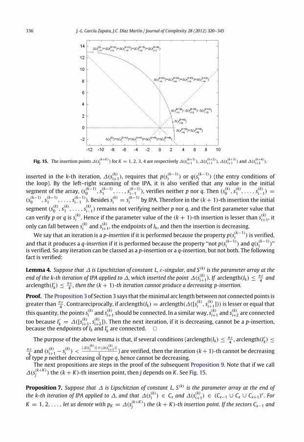
336 J.-L. García Zapata, J.C. Díaz Martín / Journal of Complexity 28 (2012) 320–345
Fig. 15. The insertion points ∆(s(k+K)j ) for K = 1, 2, 3, 4 are respectively ∆(s(k+1)
i+1 ), ∆(s(k+2)i+1 ), ∆(s(k+3)
i+1 ) and ∆(s(k+4)i+2 ).
inserted in the k-th iteration, ∆(s(k)i+1), requires that p(s(k−1)i ) or q(s(k−1)
i ) (the entry conditions ofthe loop). By the left–right scanning of the IPA, it is also verified that any value in the initialsegment of the array, (s(k−1)
0 , s(k−1)1 , . . . , s(k−1)
i−1 ), verifies neither p nor q. Then (s(k)0 , s(k)1 , . . . , s(k)i−1) =
(s(k−1)0 , s(k−1)
1 , . . . , s(k−1)i−1 ). Besides s(k)i = s(k−1)
i by IPA. Therefore in the (k + 1)-th insertion the initialsegment (s(k)0 , s(k)1 , . . . , s(k)i−1) remains not verifying neither p nor q, and the first parameter value thatcan verify p or q is s(k)i . Hence if the parameter value of the (k + 1)-th insertion is lesser than s(k)i+1, itonly can fall between s(k)i and s(k)i+1, the endpoints of Ik, and then the insertion is decreasing.
We say that an iteration is a p-insertion if it is performed because the property p(s(k−1)i ) is verified,
and that it produces a q-insertion if it is performed because the property ‘‘not p(s(k−1)i ) and q(s(k−1)
i )’’is verified. So any iteration can be classed as a p-insertion or a q-insertion, but not both. The followingfact is verified:
Lemma 4. Suppose that ∆ is Lipschitzian of constant L, ε-singular, and S(k) is the parameter array at theend of the k-th iteration of IPA applied to ∆, which inserted the point ∆(s(k)i+1). If arclength(Ik) ≤
πε4 and
arclength(I ′k) ≤πε4 , then the (k + 1)-th iteration cannot produce a decreasing p-insertion.
Proof. The Proposition 3 of Section 3 says that theminimal arc length betweennot connected points isgreater than πε
4 . Contrareciprocally, if arclength(Ik) = arclength(∆([s(k)i , s(k)i+1])) is lesser or equal thatthis quantity, the points s(k)i and s(k)i+1 should be connected. In a similar way, s(k)i+1 and s(k)i+2 are connectedtoo because I ′k = ∆([s(k)i+1, s
(k)i+2]). Then the next iteration, if it is decreasing, cannot be a p-insertion,
because the endpoints of Ik and I ′k are connected. �
The purpose of the above lemma is that, if several conditions (arclength(Ik) ≤πε4 , arclength(I ′k) ≤
πε4 and (s(k)i+1 − s(k)i ) <
|∆(s(k)i )|+|∆(s(k)i+1)|
L ) are verified, then the iteration (k+ 1)-th cannot be decreasingof type p neither decreasing of type q, hence cannot be decreasing.
The next propositions are steps in the proof of the subsequent Proposition 9. Note that if we call∆(s(k+K)
j ) the (k + K)-th insertion point, then j depends on K . See Fig. 15.
Proposition 7. Suppose that ∆ is Lipschitzian of constant L, S(k) is the parameter array at the end ofthe k-th iteration of IPA applied to ∆, and that ∆(s(k)i ) ∈ Cx and ∆(s(k)i+1) ∈ (Cx−1 ∪ Cx ∪ Cx+1)
c . ForK = 1, 2, . . . , let us denote with pK = ∆(s(k+K)
j ) the (k + K)-th insertion point. If the sectors Cx−1 and

J.-L. García Zapata, J.C. Díaz Martín / Journal of Complexity 28 (2012) 320–345 337
Cx+1 do not contain any point from p1, p2, . . . , pK , then there are a (k+K +1)-th insertion pK+1 between∆(s(k)i ) and ∆(s(k)i+1). Besides if pK is of type p then pK+1 is of type p and decreasing.
Proof. If Cx−1 and Cx+1 do not contain any point from p1, p2, . . . , pK , we have that, in the array S(k+K),the images of the values in the segment (s(k+K)
i , s(k+K)i+1 , . . . , s(k+K)
i+K+1) does not belong to Cx−1 ∪ Cx+1,and that the extreme points of this segment ∆(s(k+K)
i ) = ∆(s(k)i ) ∈ Cx and ∆(s(k+K)i+K+1) = ∆(s(k)i+1) ∈
(Cx−1 ∪Cx ∪Cx+1)c are not connected. Then at least one∆(s(k+K)
h )with i ≤ h < i+K +1 should verifyp(s(k+K)
h ), hence it is verified at least one condition inducing a (k + K + 1)-th insertion.To see that the insertion pK+1 is decreasing if pK is of type p, let us consider the points q1 =
∆(s(k+K−1)j−1 ) and q2 = ∆(s(k+K−1)
j ) that caused the insertion of pK = ∆(s(k+K)j ). They are the first
found points that verify either ‘‘q1 and q2 are in not connected sectors’’ (that is p(s(k+K−1)j−1 )), or
‘‘(s(k+K−1)j − s(k+K−1)
j−1 ) ≥|∆(s(k+K−1)
j−1 )|+|∆(s(k+K−1)j )|
L ’’ (that is q(s(k+K−1)j−1 )). Besides, from the left–right
scanning of the IPA, it is verified that the previous points (s(k+K−1)i , s(k+K−1)
i+1 , . . . , s(k+K−1)j−3 , s(k+K−1)
j−2 ) inthe array S(k+K−1) should verify ‘‘not p and not q’’, because in contrary case the (k + K)-th insertionpoint will have an index lesser then j, in contradiction with pK = ∆(s(k+K)
j ). As the points of thesegment (∆(s(k+K−1)
i+1 ), ∆(s(k+K−1)i+2 ), . . . , ∆(s(k+K−1)
j−1 ) = q1) are all from the set {p1, p2, . . . , pK } (thatis out of Cx−1 ∪ Cx+1), and ∆(s(k+K−1)
i ) = ∆(s(k)i ) ∈ Cx, and ‘‘not p(s(k+K−1)h )’’, i ≤ h < j − 1, we
deduce that all these points pertain to Cx, in particular q1 ∈ Cx. Hence, as pK is of type p (that is,p(s(k+K−1)
j−1 )), then q2 ∈ (Cx−1 ∪ Cx ∪ Cx+1)c . Finally, the point pK pertains to Cx or to (Cx−1 ∪ Cx ∪ Cx+1)
c
(by hypothesis), then the (k + K + 1)-th insertion is performed in S(k+K)= (. . . , q1, pK , q2, . . .)
between pK , q2 (if pK ∈ Cx) or between q1, pK (if pK ∈ (Cx−1 ∪ Cx ∪ Cx+1)c). In any case it is of type p
and decreasing. �
Note that, by the above proposition, the successive insertion points between s(k)i and s(k)i+1 are oftype p until one of them belongs to Cx−1 ∪ Cx+1, after which can come one or several of type q.
Proposition 8. Suppose that ∆ is Lipschitzian of constant L, ε-singular, and S(k) is the parameter array atthe end of the k-th iteration of IPA applied to∆. Calling M = (s(k)i+1 − s(k)i ), if the interval [s(k)i , s(k)i+1] verifies∆(s(k)i ) ∈ Cx and ∆(s(k)i+1) ∈ (Cx−1 ∪ Cx ∪ Cx+1)
c , then for some K ≤ ⌈lg2(4LMπε
)⌉ the (k + K)-th insertionpoint pK verifies pK ∈ Cx−1 ∪ Cx+1.
Proof. Let us define k0 as the integer verifying LM2k0
≤π4 ε ≤
LM2k0−1 , that is k0 = ⌈lg2(
4LMπε
)⌉. Ingeneral, it is not possible to have k0 + 1 consecutive decreasing p-insertions. This is because westart with a segment Ik = ∆([s(k)i , s(k)i+1]), whose arclength is lesser than LM with M = (s(k)i+1 − s(k)i ),and after k0 decreasing insertions, calling s(k+k0)
j the parameter of the (k + k0)-th insertion point
pk0 = ∆(s(k+k0)j ), we have that the endpoints parameter difference of Ik+k0 = ∆([s(k+k0)
j−1 , s(k+k0)j ])
is (s(k+k0)j − s(k+k0)
j−1 ) =M2k0
, and arclength(Ik+k0) ≤LM2k0
, that is lesser or equal than πε4 by definition of
k0. Hence by Lemma 4 the (k+ k0 + 1)-th iteration, if it is of type p, cannot be a decreasing insertion:it should be not decreasing.
Note that if for some K , lesser or equal than k0, we have that pK ∈ Cx−1 ∪ Cx+1, we concludebecause it is the claim of the proposition. In contrary case we reach a contradiction, because then foreach K from 1 to k0, pK ∈ Cx−1 ∪ Cx+1. Then we can apply Proposition 7 for K = 1 (that is, usingthe hypothesis that p1 ∈ Cx−1 ∪ Cx+1), because p1 is of type p by the hypothesis ‘‘∆(s(k)i ) ∈ Cx and∆(s(k)i+1) ∈ (Cx−1 ∪ Cx ∪ Cx+1)
c ’’, to conclude that p2 is decreasing and of type p; also for K = 2(knowing p2 ∈ Cx−1 ∪ Cx+1 and of type p) to conclude that p3 is decreasing and of type p, and so on forK = 1, 2, . . . , k0, concluding that the (k+ K)-th insertion pK (for K = 2, 3, . . . , k0 + 1) is decreasingand of type p. This is in contradiction with the above observation, that the (k + k0 + 1)-th iterationcannot be decreasing and of type p. �

338 J.-L. García Zapata, J.C. Díaz Martín / Journal of Complexity 28 (2012) 320–345
The following proposition plays a role similar to Proposition 6 (Section 4). While that one gaveus a bound for the number of insertions than can be performed until a point is inserted in a sectorconnected to that of ∆(si), Proposition 9 give us a bound for the number of insertions until a pointverifies not p and not q. Both propositions serve as basis to subsequent lemmas that bound thenumber of insertions that the processes IP and IPA perform between two parameter values. Thenumber of insertions required by IPA is greater than by IP because an insertion of type q, even inthe hypothesis of Proposition 7, can be not decreasing. Notwithstanding, the number of q-insertions
verifies the following: if ∆ is ε-singular then|∆(s(k)i )|+|∆(s(k)i+1)|
L ≥2εL because |∆(t)| ≥ ε for any
parameter t . Therefore, if it is verified q(s(k)i ) (that is, (s(k)i+1 − s(k)i ) ≥|∆(s(k)i )|+|∆(s(k)i+1)|
L , that is greater
or equal than 2εL ), then the inserted point has a parameter value s(k+1)
i+1 =s(k)i +s(k)i+1
2 that verifies
(s(k+1)i+1 − s(k)i ) =
s(k)i+1−s(k)i2 ≥
|∆(s(k)i )|+|∆(s(k)i+1)|
2L ≥εL and (s(k)i+1 − s(k+1)
i+1 ) =s(k)i+1−s(k)i
2 ≥εL . That is, s
(k+1)i+1
is located at a distance greater than εL from s(k)i and from s(k)i+1. Hence, x insertions of type q extends
over a length greater or equal than (x− 1) εL . Inside a parameter segment of lengthM (and at distance
greater than εL of its end points) the number of q-insertionsmust verify (x−1) ε
L +2 εL = (x+1) ε
L ≤ M .That is, it cannot be more than ⌊
LMε
− 1⌋q-insertions, if this expression is greater or equal than 0, orno q-insertion at all in other case.
We will denote ⌊LMε
− 1⌋0 = max(0, ⌊ LMε
− 1⌋).
Proposition 9. Suppose that ∆ is Lipschitzian of constant L, ε-singular, and S(k) is the parameter arrayat the end of the k-th iteration of IPA applied to ∆. Calling M = (s(k)i+1 − s(k)i ), if ∆(s(k)i ) ∈ Cx,∆(s(k)i+1) ∈ (Cx−1 ∪ Cx ∪ Cx+1)
c , and there are x insertions of type q in the interval [s(k)i , s(k)i+1], then for
some K ′≤ (x + 1)⌈lg2(
4LMπε
)⌉ + x there is a point s(k+K ′)g of the array S(k+K ′) verifying that ∆(s(k+K ′)
g ) ∈
Cx−1 ∪ Cx+1 and that for each h with i ≤ h < g there is not verified neither p(s(k+K ′)h ) nor q(s(k+K ′)
h ).
Proof. The formulation is more involved than Proposition 6 because the point s(k+K ′)g of interest is not
necessarily the point pK ′ inserted in the iteration (k + K ′)-th. We will prove the claim by completeinduction on x.
With x = 0, the base case, we have, by Proposition 8, that for some K ≤ ⌈lg2(4LMπε
)⌉ the (k+ K)-thinsertion point pK = ∆(s(k+K)
j ) verifies pK ∈ Cx−1 ∪Cx+1. We can suppose that this is the first insertedpoint belonging to Cx−1 ∪ Cx+1, because a previous insertion point belonging to this region will tooverify the bound. It is not verified p(s(k+K−1)
h ) for i ≤ h < j−1, because in contrary case the (k+K)-thinsertion will not have a parameter with index j. Note that, for i ≤ h < j − 1, are equivalent ‘‘notp(s(k+K−1)
h )’’ and ‘‘not p(s(k+K)h )’’, because the points involved by these asserts in S(k+K−1) and S(k+K)
are the same. Then the image points of the initial segment (s(k+K)i , s(k+K)
i+1 , . . . , s(k+K)j−2 , s(k+K)
j−1 ) of thearray S(k+K) should pertain to Cx, because they are connected (‘‘not p(s(k+K)
h )’’), and p(s(k+K)j ) is the
first insertion point pertaining to Cx−1 ∪ Cx+1. Besides, as pK belongs to Cx−1 ∪ Cx+1, it is not verifiedp(s(k+K)
h ) for h = j−1. Also it is not verified q(s(k+K)j ) for i ≤ h < j because in that casewewill have a q-
insertion, and this is not possible with x = 0. Hence we conclude the claimwith K ′= K ≤ ⌈lg2(
4LMπε
)⌉and g = j.
For x > 0, the general case, suppose that the first q-insertion is the (k + T )-th, and that y is thenumber of consecutive q-insertions that appear after this one. Thatmean that pT is the first q-insertion,and also that pT+1, pT+2, . . . until pT+y−1 are of type q, but pT+y (if it exists) is a p-insertion. ByProposition 8, we know that in nomore than K ≤ ⌈lg2(
4LMπε
)⌉ insertions, pK = ∆(s(k+K)j ) ∈ Cx−1∪Cx+1.
We have that T = K + 1, by the following reasoning: as this insertion, the (k + K)-th one, take placein the j-th entry of the array, then it is verified neither p(s(k+K−1)
h ) nor q(s(k+K−1)h ) for i ≤ h < j − 1
(this is equivalent to neither p(s(k+K)h ) nor q(s(k+K)
h ) for i ≤ h < j−1). Also, as∆(s(k+K)j ) ∈ Cx−1 ∪Cx+1,
it is not verified p(s(k+K)j−1 ). If besides it is not verified q(s(k+K)
j−1 ), we conclude with the desired claim:

J.-L. García Zapata, J.C. Díaz Martín / Journal of Complexity 28 (2012) 320–345 339
‘‘∆(s(k+K ′)g ) ∈ Cx−1 ∪ Cx+1 and for each h with i ≤ h < g there is not verified neither p(s(k+K ′)
h ) norq(s(k+K ′)
h )’’ with K ′= K ≤ ⌈lg2(
4LMπε
)⌉ and g = j, as in the base case. It left to consider that q(s(k+K)j−1 ) is
verified, but then the (k + K + 1)-th insertion is of type q, and T = K + 1.Hence there are y consecutive insertions of type q, pK+1 to pK+y, but pK+y+1 (if it exists) is of type p.
Letwe call K1 = K+y, and s(k+K1)f the parameter value of the last of this initial sequence of consecutive
q-insertions: pK1 = ∆(s(k+K1)f ). As this last insertion, the (k + K1)-th one, take place in the f -th entry
of the array, then it is verified neither p(s(k+K1−1)h ) nor q(s(k+K1−1)
h ) for i ≤ h < f − 1 (equivalently,neither p(s(k+K1)
h ) nor q(s(k+K1)h ) for i ≤ h < f −1). In addition, as the next insertion pK1+1 = pK+y+1 is
not of type q (or it not exists), it cannot be verified q(s(k+K1)f−1 ). Summarizing, we have ‘‘not p(s(k+K1)
h )’’
for i ≤ h < f − 1, and ‘‘not q(s(k+K1)h )’’ for i ≤ h ≤ f − 1. This fact will be used several times below.
Now we discuss two separate cases. We consider first that some point of the initial segment(s(k+K1)
i , s(k+K1)i+1 , . . . , s(k+K1)
f−2 , s(k+K1)f−1 ) of the array S(k+K1) has it image not pertaining to Cx. Let us call
g the lesser of this values, that is, the first index g with i ≤ g ≤ f − 1 and the image ∆(s(k+K1)g )
not pertaining to Cx. It should verify ∆(s(k+K1)g ) ∈ Cx−1 ∪ Cx+1, because we have ‘‘not p(s(k+K1)
h )’’ fori ≤ h < f − 1, hence the images of (s(k+K1)
i , s(k+K1)i+1 , . . . , s(k+K1)
g−2 , s(k+K1)g−1 ) should be on connected
sectors, and ∆(s(k+K1)g ) is the first not in Cx. And for each h with i ≤ h < g there is not verified
neither p(s(k+K1)h ) nor p(s(k+K1)
h ) (by the fact shown above ‘‘not p(s(k+K1)h )’’ and ‘‘not q(s(k+K1)
h )’’ fori ≤ h < f − 1, and g ≤ f − 1). As y ≤ x, we have a point ∆(s(k+K1)
g ) that satisfies the desiredclaim with K ′
= K1 = K + y ≤ ⌈lg2(4LMπε
)⌉ + x ≤ (x + 1)⌈lg2(4LMπε
)⌉ + x.Now we consider the alternative case, that all image points of the initial segment (s(k+K1)
i , s(k+K1)i+1
, . . . , s(k+K1)f−2 , s(k+K1)
f−1 ) of the array S(k+K1) pertain to Cx. In particular ∆(s(k+K1)f−1 ) ∈ Cx. For pK1 =
∆(s(k+K1)f ) there are the three possible options: pK1 ∈ Cx, pK1 ∈ Cx−1∪Cx+1, or pK1 ∈ (Cx−1∪Cx∪Cx+1)
c .
In the first option, as pK1 = ∆(s(k+K1)f ) ∈ Cx and ∆(s(k+K1)
i+K1+1) = ∆(s(k)i+1) ∈ (Cx−1 ∪ Cx ∪ Cx+1)c , calling
M2 = (s(k)i+1 − s(k+K1)f ), we can apply the induction hypothesis to the interval [s(k+K1)
f , s(k)i+1], that onlycan have x − y insertions of type q, and deduce that in K2 ≤ (x − y + 1)⌈lg2(
4LM2πε
)⌉ + (x − y)insertions, we have some point ∆(s(k+K1+K2)
g2) ∈ Cx−1 ∪ Cx+1 such that for each h with f ≤ h < g2
there is not verified neither p(s(k+K1+K2)h ) nor q(s(k+K1+K2)
h ). Hence we conclude with the desired claimtaking K ′
= K1 + K2 and g = g2, because as M2 ≤ M and x − y + 1 ≤ x, we have thatK1+K2 = K +y+K2 ≤ ⌈lg2(
4LMπε
)⌉+y+(x−y+1)⌈lg2(4LM2πε
)⌉+(x−y) ≤ (x+1)⌈lg2(4LMπε
)⌉+x. Alsowe have that ‘‘not p(s(k+K1+K2−1)
h ) and not q(s(k+K1+K2−1)h )’’ for i ≤ h ≤ f − 1 (because in contrary case
we do not reach the insertion ∆(s(k+K1+K2)g2 ) of index g2 with f < g2), and s(k+K1+K2−1)
h = s(k+K1+K2)h for
i ≤ h ≤ f − 1. Joining i ≤ h ≤ f − 1 with f ≤ h < g2, we have neither p(s(k+K1+K2)h ) nor q(s(k+K1+K2)
h )for each hwith i ≤ h < g2.
In the second option pK1 ∈ Cx−1 ∪ Cx+1 we also obtain that we wanted taking g = f andK ′
= K1 = K + y ≤ (x + 1)⌈lg2(4LMπε
)⌉ + x, because ∆(s(k+K1)f ) pertains to Cx−1 ∪ Cx+1, and by
the fact shown above ‘‘not p(s(k+K1)h ) and not q(s(k+K1)
h )’’ for i ≤ h < f .Finally, in the third option, pK1 ∈ (Cx−1 ∪ Cx ∪ Cx+1)
c , as ∆(s(k+K1)f−1 ) ∈ Cx and ∆(s(k+K1)
f ) ∈
(Cx−1 ∪ Cx ∪ Cx+1)c , calling M2 = (s(k+K1)
f − s(k+K1)f−1 ), we can apply the induction hypothesis to the
interval [s(k+K1)f−1 , s(k)f ], that only can have (x− y) insertions of type q, and deduce that in K2 ≤ (x− y+
1)⌈lg2(4LM2πε
)⌉+ (x− y) insertions, we have some point ∆(s(k+K1+K2)g2 ) ∈ Cx−1 ∪Cx+1 such that for each
hwith f − 1 ≤ h < g2 there is not verified neither p(s(k+K1+K2)h ) nor q(s(k+K1+K2)
h ). Similarly as before,we conclude taking K ′
= K1 +K2 = K +y+K2 ≤ ⌈lg2(4LMπε
)⌉+y+ (x−y+1)⌈lg2(4LM2πε
)⌉+ (x−y) ≤
(x + 1)⌈lg2(4LMπε
)⌉ + x and we have that ‘‘not p(s(k+K1+K2)h ) and not q(s(k+K1+K2)
h )’’ for i ≤ h < g2. �

340 J.-L. García Zapata, J.C. Díaz Martín / Journal of Complexity 28 (2012) 320–345
This proposition allows us to prove the following:
Lemma 5. Suppose that ∆ is Lipschitzian of constant L, ε-singular, and S(k) is the parameter array at theend of the k-th iteration of IPA applied to ∆, and M = (s(k)i+1 − s(k)i ) being ∆(s(k)i ) the k-th insertion point.If N is the number of borders crossed by ∆([s(k)i , s(k)i+1]), for N ≥ 2 the number of insertion points between∆(s(k)i ) and ∆(s(k)i+1) is bounded by (N − 1)(⌊ LM
ε− 1⌋0 + 1)⌈lg2(
4LMπε
)⌉ + N⌊LMε
− 1⌋0.
Proof. We prove that assert by induction on N . If N = 2, by Proposition 9, in K ′ insertions, withK ′
≤ (x + 1)⌈lg2(4LMπε
)⌉ + x, being x the number of q-insertions, we have an insertion point
∆(s(k+K ′)g ) ∈ Cx−1 ∪ Cx+1 such that for each h with i ≤ h < g there is not verified neither
p(s(k+K ′)h ) nor q(s(k+K ′)
h ). Remember that the number of q-insertions is bounded by ⌊LMε
− 1⌋0, so K ′≤
(⌊ LMε
− 1⌋0+1)⌈lg2(4LMπε
)⌉+⌊LMε
− 1⌋0. As it is verified ‘‘neither p nor q’’, the IPAwill not produce any
additional insertion in the curve segment ∆([s(k)i , s(k+K ′)g ]). Besides it will not produce any p-insertion
in ∆([s(k+K ′)g , s(k)i+1]) (because the end points are connected as N = 2). The number of q-insertions
in ∆([s(k+K)g , s(k)i+1]) is bound by ⌊
L(s(k)i+1−s(k+K)g )
ε− 1⌋0 ≤ ⌊
LMε
− 1⌋0, hence the total of insertions in∆([s(k)i , s(k)i+1]) is lesser or equal than K ′
+ ⌊LMε
− 1⌋0 ≤ (⌊ LMε
− 1⌋0 + 1)⌈lg2(4LMπε
)⌉ + 2⌊ LMε
− 1⌋0,that is our claim.
For the general case N > 2, the hypothesis of induction is that any curve segment, with endpointsparameter difference of M ′, crossing (N − 1) borders requires at most (N − 2)(⌊ LM ′
ε− 1⌋0 +
1)⌈lg2(4LM ′
πε)⌉ + (N − 1)⌊ LM ′
ε− 1⌋0. By Proposition 9, for a K ′ lesser or equal than K ′
≤ (x +
1)⌈lg2(4LMπε
)⌉ + x ≤ (⌊ LMε
− 1⌋0 + 1)⌈lg2(4LMπε
)⌉ + ⌊LMε
− 1⌋0, we have that an insertion point
∆(s(k+K ′)g ) ∈ Cx−1 ∪ Cx+1 such that for each h with i ≤ h < g there is not verified neither p(s(k+K ′)
h )
nor q(s(k+K ′)h ). Then the segment ∆([s(k)i , s(k+K ′)
g ]) will not have more insertions, and ∆([s(k+K ′)g , s(k)i+1]),
with endpoints parameter difference ofM ′= (s(k)i+1−s(k+K ′)
g ) < M by induction hypothesis, requires atmost (N−2)(⌊ LM ′
ε− 1⌋0+1)⌈lg2(
4LM ′
πε)⌉+(N−1)⌊ LM ′
ε− 1⌋0 ≤ (N−2)(⌊ LM
ε− 1⌋0+1)⌈lg2(
4LMπε
)⌉+
(N − 1)⌊ LMε
− 1⌋0 insertions. Adding the bounds of both segments, we have that the total is lesser orequal than (N − 1)(⌊ LM
ε− 1⌋0 + 1)⌈lg2(
4LMπε
)⌉ + N⌊LMε
− 1⌋0. �
Finally we have:
Theorem 4. If ∆ : [a, b] → C is ε-singular with ε = 0, with a Lipschitzian parameterization of constantL, then the IPA for the curve ∆ concludes in less than 4L(b−a)
πε(⌊
L|S(0)|
ε− 1⌋0 + 1)⌈lg2(
4L|S(0)|
πε)⌉+ (
4L|S(0)|
πε+
1)⌊ L(b−a)ε
− 1⌋0 insertions.
Proof. The number N of borders crossed by each segment ∆([s(0)i , s(0)i+1]) of the initial array are such
that N − 1 ≤4L(s(0)i+1−s(0)i )
πε, as viewed in the proof of Theorem 2. Applying the previous lemma we
have that the maximum number of insertions in each segment is4L(s(0)i+1−s(0)i )
πε(⌊
L(s(0)i+1−s(0)i )
ε− 1⌋0 + 1)
⌈lg2(4L(s(0)i+1−s(0)i )
πε)⌉ + (
4L(s(0)i+1−s(0)i )
πε+ 1)⌊
L(s(0)i+1−s(0)i )
ε− 1⌋0. Adding these values, as lg2(
4L(s(0)i+1−s(0)i )
πε) ≤
lg2(4L|S(0)
|
πε), ⌊
L(s(0)i+1−s(0)i )
ε− 1⌋0 ≤ ⌊
L|S(0)|
ε− 1⌋0 and
n−1i=0 ⌊
L(s(0)i+1−s(0)i )
ε⌋ ≤ ⌊
n−1i=0
L(s(0)i+1−s(0)i )
ε⌋ =
⌊L(b−a)
ε⌋, we have that the total of insertions are lesser or equal than 4L(b−a)
πε(⌊
L|S(0)|
ε− 1⌋0 + 1)
⌈lg2(4L|S(0)
|
πε)⌉ +(
4L|S(0)|
πε+ 1)⌊ L(b−a)
ε− 1⌋0. �
Note that this bound of the number of insertions required by IPA for an winding numbercomputation is of order O( 1
ε2lg2(
1ε) +
1εlg2(
1ε)) = O( 1
ε2lg2(
1ε)).

J.-L. García Zapata, J.C. Díaz Martín / Journal of Complexity 28 (2012) 320–345 341
Fig. 16. The point D is at the same distance from the origin as ∆(si+2).
6. Bound of cost regardless of the ε-singularity
Using IPA procedure, an index computation requires 4L(b−a)πε
(⌊L|S(0)
|
ε− 1⌋0 + 1) ⌈lg2(
4L|S(0)|
πε)⌉ +
(4L|S(0)
|
πε+ 1)⌊ L(b−a)
ε− 1⌋0 insertions. However, if ε is not known, this formula cannot be applied to
foresee the number of insertions required. It can be arbitrarily high if the distance from the curve∆ tothe origin is near to 0. The IPA, applied to a curve with unknown value of singularity ε, is confrontedto an unpredictable cost. To control this, we modify the IPA, in such a way that we can bound the costof the index computation, returning with error if this bound is exceeded. The tool used is Theorem 5below. It is based on the fact that two insertion points with near parameter values imply a low valueof singularity. We first proof this for p-insertions, in Lemma 3, and then for q-insertions in Lemma 4.
Lemma 6. If si, si+1, si+2 are three parameter values of the curve ∆, Lipschitzian with constant L,ε-singular, and si+1 verifies that si+1 =
si+si+22 with ∆(si) and ∆(si+2) in non-connected sectors, and
besides si+1 − si ≤ δ for a positive δ, then either |∆(si)| or |∆(si+2)| are lesser or equal than Lδsin( π
8 ).
Consequently ε ≤Lδ
sin( π8 )
.
Proof. As si+1 =si+si+2
2 then si+2−si+1 = si+1−si and by hypothesis si+2−si = si+2−si+1+si+1−si =
2(si+1 − si) ≤ 2δ. Besides by the Lipschitz property, |∆(si+2) − ∆(si)| ≤ L(si+2 − si) ≤ L2δ. Then wehave that the points ∆(si) and ∆(si+2) are in non-connected sectors, but at a distance lesser than L2δ.Let us consider the triangle formed by these points and the origin O. It has an angle α at O greater thanπ4 , but lesser or equal than π because is the internal angle of a triangle. The opposite side to α is thesegment ∆(si)∆(si+2), of length lesser or equal than L2δ (see Fig. 16). We will show that either ∆(si)or∆(si+2) are at a distance lesser or equal than Lδ
sin( π8 )
from the origin. Suppose that |∆(si+2)| ≤ |∆(si)|
(in case that |∆(si+2)| > |∆(si)|, the reasoning is similar). Let D be the point of the segment O∆(si) atthe same distance from O that ∆(si+2).
It is verified that length(∆(si+2)D) ≤ L2δ, because the isosceles triangle of vertices O, ∆(si+2), Dhas the minimum side between those triangles having an angle of α and whose lesser adjacent sidehas length |∆(si+2)|. Besides, considering the right triangle that arises from the α angle bisector, we
have that sin( α2 ) =
length(∆(si+2)D)
2|∆(si+2)|
. Finally note that as π4 ≤ α ≤ π , then π
8 ≤α2 ≤
π2 and therefore
π8 and α
2 are in an increasing interval of the sine function, and verify sin(π8 ) ≤ sin( α
2 ). Chaining theseinequalities we have:
sinπ
8
≤ sin
α
2
=
length(∆(si+2)D)
2
|∆(si+2)|≤
Lδ|∆(si+2)|
.

342 J.-L. García Zapata, J.C. Díaz Martín / Journal of Complexity 28 (2012) 320–345
And then |∆(si+2)| ≤Lδ
sin( π8 )
. As ε is theminimum |∆(s)| for s ∈ [a, b], we have that ε ≤ |∆(si+2)| ≤
Lδsin( π
8 ). �
Lemma 7. If S = (s0, . . . , sm) is an array of parameter values of the curve ∆, Lipschitzian with constantL, with value of singularity ε, and si+1 verifies that si+1 =
si+si+22 with (si+2 − si) ≥
|∆(si)|+|∆(si+2)|L ,
and besides si+1 − si ≤ δ for a positive δ, then either |∆(si)| or |∆(si+2)| are lesser or equal than Lδ. Asconsequence ε ≤ Lδ.
Proof. As si+1 =si+si+2
2 then si+2 − si+1 = si+1 − si and by hypothesis, as in Lemma 6, si+2 − si =
si+2 − si+1 + si+1 − si = 2(si+1 − si) ≤ 2δ. Chaining this with (si+2 − si) ≥|∆(si)|+|∆(si+2)|
L ,we have 2δ ≥
|∆(si)|+|∆(si+2)|L , that is 2Lδ ≥ |∆(si)| + |∆(si+2)| ≥ 2min(|∆(si)|, |∆(si+2)|). Then
min(|∆(si)|, |∆(si+2)|) ≤ Lδ, that implies the conclusion. �
Note that the lemmas are valid for any three parameter values. In particular, if s(k)i+1 is the value
inserted in a iteration of the IPA in the array S(k)= (s(k)0 , s(k)1 , . . . , s(k)n+k), then s(k)i+1 =
s(k−1)i +s(k−1)
i+12 =
s(k)i +s(k)i+22 . Then we have that:
Corollary. If S(k)= (s(k)0 , s(k)1 , . . . , s(k)n+k) is the state of the array at the end of any iteration of the IPA, and
if ∆(s(k)i+1) is the last insertion point, with s(k)i+1 − s(k)i ≤ δ for a positive δ, then ε ≤Lδ
sin( π8 )
.
Proof. Note that, in the k-th iteration of the while loop, the conditions p and q are evaluated onthe array S(k−1) resulting from the previous iteration. Then it is verified than ‘‘p(s(k−1)
i ) or q(s(k−1)i )’’,
and the point inserted has as parameter s(k)i+1 =s(k−1)i +s(k−1)
i+12 =
s(k)i +s(k)i+22 . On one hand, if p(s(k−1)
i ),then ∆(s(k−1)
i ) = ∆(s(k)i ) and ∆(s(k−1)i+1 ) = ∆(s(k)i+2) are not connected, and the values s(k)i , s(k)i+1 and
s(k)i+2 are in the hypothesis of Lemma 6. Therefore ε ≤Lδ
sin( π8 )
. On the other hand, if q(s(k−1)i ), then
(s(k−1)i+1 − s(k−1)
i ) ≥|∆(s(k−1)
i )|+|∆(s(k−1)i+1 )|
L , i.e. (s(k)i+2 − s(k)i ) ≥|∆(s(k)i )|+|∆(s(k)i+2)|
L , and we can apply Lemma 7to conclude that ε ≤ Lδ, that is lesser than Lδ
sin( π8 )
. In any case, if p(s(k−1)i ) or q(s(k−1)
i ), and s(k)i+1−s(k)i ≤ δ,
then we have that ε ≤Lδ
sin( π8 )
. �
With this bound of the value of singularity ε (that ε ≤Lδ
sin( π8 )
if s(k)i+1 − s(k)i ≤ δ at the insertion of
s(k)i+1), we modify the IPA in such a way that we can bound the number of iterations performed. Theinsertion procedure with control of singularity (IPS) (showed in Fig. 17) has as inputs an analyticallydefined curve ∆, an array S(0)
= (s(0)0 , s(0)1 , . . . , s(0)n ) and a real parameter Q . Remember that S(k)=
(s(k)0 , s(k)1 , . . . , s(k)n+k) is the value of the parameter array after k-th insertion. The assertions p(s(k)i ) andq(s(k)i ) are like in the previous section, and r(s(k)i ,Q ) is ‘‘the values s(k)i and s(k)i+1 in array S(k) verifys(k)i+1 − s(k)i ≤ Q ’’.
Informally, we can say that the insertion procedure with control of singularity involves a whileloop that is repeated until a connected array (i.e., verifying the condition ‘‘no p’’) and without lostturns (‘‘no q’’) is obtained, checking (with r) that it does not run forever.
Note that the assertion r(s(k)i , δ) is equivalent to s(k)i+1 − s(k)i ≤ δ, the hypothesis of the abovecorollary, and in case of return on error we can apply it to deduce an upper bound on the value ofsingularity.
The usage of the output array to compute Ind(∆), and the cost of the IPS, is described by thefollowing:
Theorem 5. If ∆ : [a, b] → C is Lipschitzian with constant L, S(0) an array sampling of [a, b], and Q apositive real, the insertion procedure with control of singularity applied to ∆, S(0) and Q verifies:

J.-L. García Zapata, J.C. Díaz Martín / Journal of Complexity 28 (2012) 320–345 343
Fig. 17. Insertion procedure with control of singularity (IPS). Note that the ‘‘Insert’’ line produces S(k) from S(k−1) in the k-thiteration.
(a) Returns in less than ⌊b−aQ − 1⌋
0iterations.
(b) If it exits normally then the returning array gives us Ind(∆).(c) If it exits on error, the parameter value t verifies |∆(t)| ≤
LQsin( π
8 ).
Proof. We will bound the number of parameter values inserted between a and b beginning fromthe minimal starting array (a = s(0)0 , s(0)1 = b). At the end of each iteration, the values (a =
s(k)0 , s(k)1 , . . . , s(k)k+1 = b) should verify s(k)i+1 − s(k)i ≤ Q , because in contrary case the error conditioncauses an exit. To count the maximum number of values s(k)i that we can have with that condition,let us consider that in an interval of length b − a, we can insert m values with a difference greater orequal than Q if (m + 1)Q ≤ b − a, without count the endpoints. Hence the number k of inner pointss(k)1 , . . . , s(k)k should verifies (k + 1)Q ≤ b − a, and the maximum value for k is ⌊
b−aQ − 1⌋
0. Then at
most ⌊ b−aQ − 1⌋
0iterations are performed until the error condition r(s(k)i ,Q ) is reached, if there is not
a normal exit before.For (b), the case of normal ending, the trace of execution of IPS coincides with that of IVA, and then
the returned array is valid to compute Ind(∆) by Theorem 4.Regarding the parameter value t returned on error, note that in such case it is verified that ‘‘p(s(k−1)
i )
or q(s(k−1)i ), and r(s(k)i ,Q )’’, that are the conditions required to enter the loop and to exit with error.
In case that it is verified ‘‘p(s(k−1)i ) and r(s(k)i ,Q )’’, this last iteration has been a p-iteration (that
is, s(k)i+1 =s(k)i +s(k)i+2
2 with ∆(s(k)i ) and ∆(s(k)i+2) in non-connected sectors) and s(k)i+1 − s(k)i ≤ Q . ByLemma 6, we have that either |∆(s(k)i )| or |∆(s(k)i+2)| is lesser or equal than LQ
sin( π8 )
. In case that it is
verified ‘‘q(s(k−1)i ) and r(s(k)i ,Q )’’, the last iteration has been a q-iteration (that is, s(k)i+1 =
s(k)i +s(k)i+22 with
(s(k)i+2 − s(k)i ) ≥|∆(s(k)i )|+|∆(s(k)i+2)|
L ) and s(k)i+1 − s(k)i ≤ Q . Hence by Lemma 7 either |∆(s(k)i )| or |∆(s(k)i+2)|
is lesser than LQ . As t is just t = s(k)i or t = s(k)i+1 depending on min(|∆(s(k)i )|, |∆(s(k)i+1)|), in any of thetwo cases the return value t verifies |∆(t)| ≤
LQsin( π
8 ). �
The insertion procedure with control of singularity prevents an excessive number of iterations,controlled by input parameter Q . The IPS effectively computes the index of curves ∆ with ε > LQ
sin( π8 )
,but if the value of singularity is under this level, the procedure can return with error, signaling thisfact, or can return normally with an array whose crossing number is valid to compute the index of thecurve, always in less than ⌊
b−aQ − 1⌋
0iterations.

344 J.-L. García Zapata, J.C. Díaz Martín / Journal of Complexity 28 (2012) 320–345
7. Conclusions
We have developed an algorithm for winding number computation, using discretization of thecurve to obtain an array to which the method of twist counting of Henrici can be reliably applied.We also provide a bound of its computational cost in non singular cases, in Theorem 4. This boundis of order O( 1
ε2log( 1
ε)) evaluations of the curve, being ε its minimum distance from origin. We also
provide another algorithm for winding number computation that can be applied to curves whosethis minimum distance is unknown, but assuring that, before expending a predefined amount ofcomputation, it will return either with the winding number or with an indication that the curve isnear to singular.
About connections with other works, and suggestions for future development, we can say that thecost O( 1
ε2log( 1
ε)) is coherent with the procedures analyzed in [4], that depend on a parameter n to
compute the winding number for curves with value of singularity greater than 2−n.For a class of problems, the condition number of a specific problem measures its difficulty of
resolution. The reciprocal of value of singularity, 1ε, can be viewed as a ‘‘condition number’’ similar
to that used in Matrix Numerical Analysis. This analogy of 1εwith a condition number is remarked by
the fact that it is the distance from∆ to the nearest ill-posed input data, for a suitablemetric defined inthe space of plane curves. Intuitively, it is the proximity of the specific problem to an ill-posed problemof the class (see [6,3]). In our case, an ill-posed problem is a curve that crosses over the origin, withouta defined winding number.
References
[1] Keith Ball, An elementary introduction to modern convex geometry, in: Flavors of Geometry, in: Math. Sci. Res. Inst. Publ.,vol. 31, Cambridge Univ. Press, Cambridge, 1997, pp. 1–58.
[2] Dario Bini, Victor Y. Pan, Polynomial and Matrix Computations, Vol. 1, Progress in Theoretical Computer Science,Birkhäuser Boston Inc., Boston, MA, 1994, Fundamental Algorithms.
[3] Lenore Blum, Felipe Cucker, Michael Shub, Steve Smale, Complexity and Real Computation, Springer-Verlag, New York,1998, With a foreword by Richard M. Karp.
[4] Arthur W. Chou, Ker-I Ko, Computational complexity of two-dimensional regions, SIAM J. Comput. 24 (5) (1995)923–947.
[5] G.E. Collins, Infallible calculation of polynomial zeros to specified precision, in: Mathematical Software, III (Proc. Sympos.,Math. Res. Center, Univ. Wisconsin, Madison, Wis., 1977), in: Publ. Math. Res. Center, vol. 39, Academic Press, New York,1977, pp. 35–68.
[6] James Weldon Demmel, On condition numbers and the distance to the nearest ill-posed problem, Numer. Math. 51 (3)(1987) 251–289.
[7] J.L. García Zapata, J.C Díaz Martín, A geometrical root findingmethod for polynomials, with complexity analysis, TechnicalReport, Departamento de Matemáticas, Universidad de Extremadura, 2008.
[8] Juan-Luis García Zapata, Juan Díaz Martín, Pedro Gómez Vilda, Parallel root-finding method for lpc analysis of speech,in: Petr Sojka, Ivan Kopecek, Karel Pala (Eds.), Text, Speech and Dialogue, in: Lecture Notes in Computer Science, vol. 3206,Springer, Berlin, Heidelberg, 2004, pp. 529–536. doi:10.1007/978-3-540-30120-2.
[9] Peter Henrici, Applied and Computational Complex Analysis, Vol. 1, Wiley Classics Library, John Wiley & Sons Inc.,New York, 1988, Power series-integration-conformal mapping-location of zeros, Reprint of the 1974 original, A Wiley-Interscience Publication.
[10] Donald E. Knuth, TheArt of Computer Programming, Vol. 2, second edition, Addison-Wesley Publishing Co., Reading,Mass.,1981, Seminumerical Algorithms, Addison-Wesley Series in Computer Science and Information Processing.
[11] A.N. Kolmogorov, S.V. Fomın, Introductory Real Analysis, Dover Publications Inc., New York, 1975, Translated from thesecond Russian edition and edited by Richard A. Silverman, Corrected reprinting.
[12] K.H. Ko, T. Sakkalis, N.M. Patrikalakis, A reliable algorithm for computing the topological degree of a mapping in R2 , Appl.Math. Comput. 196 (2) (2008) 666–678.
[13] P. Kravanja, M. Van Barel, A derivative-free algorithm for computing zeros of analytic functions, Computing 63 (1) (1999)69–91.
[14] H.J. Orchard, R.S. Elliott, G.J. Stern, Optimising the synthesis of shaped beam antenna patterns, IEE Proc. H 132 (1) (1985)63–68.
[15] Victor Y. Pan, Solving a polynomial equation: some history and recent progress, SIAM Rev. 39 (2) (1997) 187–220.[16] James Renegar, On theworst-case arithmetic complexity of approximating zeros of polynomials, J. Complexity 3 (2) (1987)
90–113.[17] G.A. Sitton, C.S. Burrus, J.W. Fox, S. Treitel, Factoring very-high-degree polynomials, IEEE Signal Process. Mag. 20 (6) (2003)
27–42.[18] R.C. Snell, F. Milinazzo, Formant location from lpc analysis data, IEEE Trans. Speech Audio Process. 1 (2) (1993)
129–134.
J.-L. García Zapata, J.C. Díaz Martín / Journal of Complexity 28 (2012) 320–345 345
[19] Toshio Suzuki, Tomohiro Suzuki, A globally convergent zero finding method, in: Proceedings of the Third World Congressof Nonlinear Analysts, Part 6 (Catania, 2000) vol. 47, 2001, pp. 3869–3875.
[20] Herbert S.Wilf, A global bisection algorithm for computing the zeros of polynomials in the complex plane, J. Assoc. Comput.Mach. 25 (3) (1978) 415–420.
[21] J.-C. Yakoubsohn, Numerical analysis of a bisection–exclusion method to find zeros of univariate analytic functions,J. Complexity 21 (5) (2005) 652–690.
[22] Xingren Ying, I. Norman Katz, A reliable argument principle algorithm to find the number of zeros of an analytic functionin a bounded domain, Numer. Math. 53 (1–2) (1988) 143–163.


![Numerical Robustness in Geometric Computation: An ...implementing geometric computations or dealing with the non-robustness problems in geometric computation have beendeveloped,includingCGAL[19],LEDA[20],CORE](https://img.pdfslide.net/doc/110x75/60d7764524dad8126a3604a1/numerical-robustness-in-geometric-computation-an-implementing-geometric-computations.jpg)