A GIS Based Emissions Estimation System For Wildfire And Prescribed Burning

Nicholas Clinton*, James Scarborough#, Yong Tian*, Peng Gong* * Center for the Assessment and Monitoring of Forest and Environmental Resources (CAMFER).

University of California, Berkeley. 94720. Tel: 510.643.4539. Email: nclinton@nature.berkeley.edu # Air Sciences Inc. 12596 W Bayaud Ave #380, Lakewood, Colorado. 80228. Tel: 303.988.2960 ABSTRACT: Emissions from wildfires and prescribed burning are difficult to measure, yet

contribute a large amount of particulate and gaseous pollutants to California air basins. This paper describes an Emissions Estimation System (EES) for the quantification and spatial allocation of wildland fire emissions based on spatial inputs and an existing fire effects model. The fuel consumption and emissions estimation algorithms from the Forest Service First Order Fire Effects Model (FOFEM, Reinhart et al. 1997) were coded in Avenue, the ArcView (ESRI) scripting language to iteratively run over multiple vegetation types and fire perimeter inputs. From PM2.5, PM10 and CO estimation, the emissions module was expanded to produce estimates for CH4, non-methane hydrocarbons, NH3, N2O, NOX, and SO2. The modularity of the EES allows it to run using a variety of spatial inputs including California Gap Analysis Program (GAP) vegetation, the Calveg dataset, and the National Fire Danger Rating System (NFDRS) fuel model map. Fire detections can be input in raster or vector format. The EES is implemented through the ArcView graphic user interface, allowing the user to specify data inputs and environmental conditions. Output of emissions mass, in either vector or raster data format, is spatially and temporally allocated (based on input data) for direct inclusion in emissions inventories. The EES is fully adaptable to multiple spatial scales depending on the scope and quality of the input data. Because the output data are geo-referenced, the EES takes advantage of GIS for the organization and storage of emission information.

INTRODUCTION

Wildland fires can be a significant contributor of pollutant emissions to the atmosphere, contributing

to decreased air quality on a continental scale (Conrad and Ivanova 1997, Fearnside 2000, Dennis et al. 2002, Amiro et al. 2001, Davies and Unam 1999, Bravo et al. 2002). In the Western United States, the contribution of wildland fires has been estimated at between 3-10% of total PM2.5 particulate emissions annually (Dickson et al. 1997, California Air Resources Board 2002). However, the impact from fires is episodic, with high temporal (seasonal and inter-annual) variability in magnitude (Grand Canyon Visibility Transportation Commission 1996, Dickson et al. 1997). For this reason, annual averages often understate the importance of the wildland fire contribution of emissions to the environment (California Air Resources Board 2002). Information about the temporal allocation of fire events should be coupled with emissions information in order to accurately depict fire contributions in the overall emissions picture.

The spatial allocation of fire events is equally important. Variability of the spatial location of fires

can influence fire effects (such as smoke production) through fuel characteristics (Keane et al. 2001, Andrews and Queen 2001, Andersen 1982). Additionally, fire location information is necessary for synthesizing emissions source models with dispersion models or other decision support systems (Sandberg et al. 1999, Battye and Battye 2002). Spatial referencing of fires is also essential to the formulation of any geographically based emission inventory.

The quantification and inventory of emissions can be a very complex process (Air Sciences, Inc.

2002). Fire emissions have been quantified using remote sensing approaches (Griffith et al. 1991, Cofer

et al. 1991), aerial sampling (Einfeld et al. 1991, Radke et al. 1991, Cofer et al. 1991), ground based sampling (Bravo et al. 2002, Susott et al. 1991, Davies and Unam 1999), and estimation from form based activity records (Dennis et al. 2002, Bravo et al. 2002, Amiro et al. 2001, Air Sciences, Inc. 2002). In general, the estimation approach makes use of a previously computed emission factor (EF) in the form of:

Eq. (1) EF = Mass of pollutant emission/Mass of fuel consumed The total emission mass of pollutant X from a fire event is then calculated as: Eq. (2) MassX = Area* Fuel loading per area*Fraction of fuel consumed*EFX This estimation protocol is commonly applied (Air Sciences Inc. 2002, California Air Resources

Board 2002, Einfeld et al. 1991, Dennis et al. 2002, Bravo et al. 2002, Amiro et al. 2001) with minor variations and enhancements. In particular, it is worth noting that the decomposition of burning into �flaming� and �smoldering� phases affects the rate, quality and quantity of emissions. In response to this change in emission quality over the duration of the burn, emission factors have been temporally resolved by combustion phase (Ward and Hardy 1991, Susott et al. 1991, Einfeld et al. 1991, Fearnside 2000). Based on relative duration of the combustion phases, weighted averages can be used to create composite emissions factors (Reinhardt et al. 1997). A large amount of work has gone into the elucidation of these pyrolytic subtleties (Battye and Battye 2002).

The Emission Estimation System (EES) described here uses an existing fuel consumption and

emission estimation model (First Order Fire Effects Model 4.0, FOFEM, Reinhardt et al. 1997), a Geographic Information System (ArcView 3.2, ESRI 1999), and public domain fire and vegetation data (California Department of Forestry and Fire Protection 2001, Burgan et al. 1998, Davis et al. 1998) to automate the estimation process described above. The fire team at the Center for the Assessment and Monitoring of Forest and Environmental Resources (CAMFER) at the University of California, Berkeley�s College of Natural Resources designed this EES under contract by the California Air Resources Board (CARB) for the purpose of wildland fire emissions estimation in the state of California (Scarborough et al. 2001). We have since expanded the system to have a national scope and include more pollutant emissions estimates. The system is intended to function as a �tool� that is readily updated or customized as the need arises. This paper will describe the tool and present a case study to illustrate its capabilities and limitations.

METHODS System We designed the EES to have the following properties:

• An adaptive architecture that can be readily modified or updated. • Spatially allocated inputs including vegetation and fire polygons. • The application of standard (non-spatial) emissions estimation models. • Spatially allocated output as tables and maps. • A flexible interface that can be customized to the needs of the user.

In order to create a system that meets these objectives, we employed a modular approach. This

allows greater utility to test different inputs, interfaces, models and other system components. We designed the system with flexibility in order to preserve the ability to switch inputs, emission factors, fuel models, or user interfaces with a minimum of system modification.

The system is based on the following modules, illustrated by Figure 1: • Dialog driven user interface to facilitate data and parameter input. • Fire area input, either vector or raster. • Vegetation or fuel map input. • Table of emission factors. • Table of fuel models with fuel loading values. • Avenue scripting of FOFEM algorithms for fuel consumption and emissions estimation.

Figure 1. Flowchart depicting the interaction of the EES modules in ArcView. The fire input and vegetation and fuel models are upper left, FOFEM based fuel consumption and emissions estimation scripts at bottom, input and output are upper right. Arrows indicate direction of processing.

The system runs entirely within ArcView GIS (Windows or Unix platforms) making use of Avenue,

the ArcView scripting language. The advantage of this approach is that Avenue is composed in a development environment that provides access to a spatial database, geographic processing functions, standard mathematical processing functions, and input of data through a graphic user interface. The user input, fuel consumption, emissions estimation, and reporting modules are all implemented in Avenue.

The EES is capable of running over a variety of inputs. Grid based processing is possible using

inputs of a fire detection grid converted to a lattice or polygons converted to centroids and the Forest Service NFDRS fuel model map, in grid format (Burgan et al. 1998). In order to perform this type of processing, CAMFER created a �crosswalk� of FOFEM fuel models to NFDRS fuel models. The EES, running in this configuration, utilizes a lower resolution fuel map (compared to the vegetation inputs), but adds the capability of estimating emissions at a national scope. This paper will describe polygon processing capability for California, using a case study as an example.

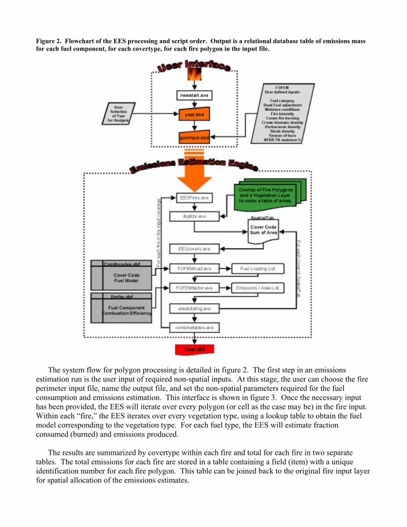
Figure 2. Flowchart of the EES processing and script order. Output is a relational database table of emissions mass for each fuel component, for each covertype, for each fire polygon in the input file.

The system flow for polygon processing is detailed in figure 2. The first step in an emissions

estimation run is the user input of required non-spatial inputs. At this stage, the user can choose the fire perimeter input file, name the output file, and set the non-spatial parameters required for the fuel consumption and emissions estimation. This interface is shown in figure 3. Once the necessary input has been provided, the EES will iterate over every polygon (or cell as the case may be) in the fire input. Within each �fire,� the EES iterates over every vegetation type, using a lookup table to obtain the fuel model corresponding to the vegetation type. For each fuel type, the EES will estimate fraction consumed (burned) and emissions produced.

The results are summarized by covertype within each fire and total for each fire in two separate

tables. The total emissions for each fire are stored in a table containing a field (item) with a unique identification number for each fire polygon. This table can be joined back to the original fire input layer for spatial allocation of the emissions estimates.

Figure 3. The EES PC interface. This dialog is invoked when the user presses a button in the ArcView toolbar. The interface allows the selection of a fire input file, a type of processing, and the input of non-spatial parameters.

Fuel Consumption and Emissions Estimation The fuel consumption and emissions estimation algorithms are implemented in Avenue and based on

published equations used in the FOFEM model documentation (Reinhardt et al. 1997). In predicting fuel consumption in �natural� settings (meaning not pile burning or broadcast burning of logging slash) and estimating emissions, the EES uses only part of the FOFEM model functionality. Emissions are the only fire effect that the EES can compute. We manually created dBASE format tables of published FOFEM fuel models and emission factors (for CO, PM10, and PM2.5) for use as input to the EES.

The fuel models contain pre-burn loadings, in tons per acre, over several live and dead fuel

categories. Live fuels have �sparse,� �typical,� and �abundant� categories that are selected based on the non-spatial user inputs to the EES. In order to make the model useful over a wide range of vegetation inputs, we �crosswalked� the fuel models to specific vegetation types. These crosswalks are stored as lookup tables for each vegetation layer. Modification of the fuel model assignments or fuel loadings within the models is possible by updating the lookup table without altering the EES.

Fuel consumption is based on the algorithms published in Reinhardt et al. (1997). We coded in

Avenue the equations that use the NFDR-TH moisture value as input. The NFDR-TH (thousand hour fuel moisture) is a non-spatial user input to the EES. We have added the capability to the EES of accepting a spatial input as a grid of NFDR-TH values, but this functionality is constrained by lack of input data. Current availability of NFDR-TH grids limits the complete implementation of this function to the EES.

Emissions estimation is based on a lookup table of emission factors in units of pounds of pollutant

per ton of fuel consumed. There are separate emission factors for each fuel component and �wet,� �moderate,� and �dry� moisture conditions. Like the fuel loadings, the set of emission factors used is based on the non-spatial user input of a moisture regime. Unlike the NFDR-TH input, which affects fuel consumption, the moisture-condition input affects emissions production. While it would be illogical to select a low NFDR-TH moisture percentage and a �wet� moisture regime, we retained the separation of the inputs in order to preserve model flexibility.

The �stock� FOFEM emissions estimated include CO, PM10, and PM2.5. We expanded the number of pollutants estimated by the EES using an �emissions ratio� approach (Lobert et al. 1991). The products of combustion are a function of combustion efficiency (Ward and Hardy 1991, Einfeld et al. 1991). Some compounds, such as CO2, have a positive correlation with combustion efficiency and others, such as CO have a negative correlation (Battye and Battye 2001, Radke et al. 1991, Lobert et al. 1991, Ward and Hardy 1991). We used ratios to either CO or CO2 depending on these relationships and whether a compound was more closely associated with �flaming� or �smoldering� combustion to expand the FOFEM table of emission factors. Table 1 displays these emission factors. This table is merely a stylized version of the emission factor table that functions as a module in the EES.

Table 1. Table of emission factors used in the EES for different moisture conditions. Emission factors for CO, PM10, and PM2.5 were obtained from FOFEM literature. All other emission factors were derived by CAMFER for use in the EES.

Pollutant Moisture Regime

Litter, Wood

0-1 inch Wood

1-3 inches Wood

3+ inches Herb, shrub,

regen Duff Canopy fuels emission factor in pounds of emissions per ton of fuel consumed

PM10 Wet 9.30 14.00 26.60 25.10 28.20 25.10 PM10 Moderate 9.30 14.00 21.60 25.10 30.40 25.10 PM10 Dry 9.30 14.00 19.10 25.10 30.40 25.10 PM25 Wet 7.90 11.90 22.50 21.30 23.90 21.30 PM25 Moderate 7.90 11.90 18.30 21.30 25.80 21.30 PM25 Dry 7.90 11.90 16.20 21.30 25.80 21.30

CO Wet 52.40 111.40 268.90 249.20 288.60 249.20 CO Moderate 52.40 111.40 205.80 249.20 316.10 249.20 CO Dry 52.40 111.40 174.40 249.20 316.10 249.20

CH4 Wet 2.10 4.46 10.76 9.97 11.54 9.97 CH4 Moderate 2.10 4.46 8.23 9.97 12.64 9.97 CH4 Dry 2.10 4.46 6.98 9.97 12.64 9.97

TNMHC Wet 3.67 7.80 18.82 17.44 20.20 17.44 TNMHC Moderate 3.67 7.80 14.41 17.44 22.13 17.44 TNMHC Dry 3.67 7.80 12.21 17.44 22.13 17.44

NH3 Wet 0.52 1.11 2.69 2.49 2.89 2.49 NH3 Moderate 0.52 1.11 2.06 2.49 3.16 2.49 NH3 Dry 0.52 1.11 1.74 2.49 3.16 2.49 N2O Wet 0.49 0.47 0.43 0.43 0.42 0.43 N2O Moderate 0.49 0.47 0.45 0.43 0.42 0.43 N2O Dry 0.49 0.47 0.45 0.43 0.42 0.43 NOX Wet 8.23 7.97 7.27 7.36 7.19 7.36 NOX Moderate 8.23 7.97 7.55 7.36 7.07 7.36 NOX Dry 8.23 7.97 7.69 7.36 7.07 7.36 SO2 Wet 2.53 2.45 2.24 2.27 2.21 2.27 SO2 Moderate 2.53 2.45 2.33 2.27 2.18 2.27 SO2 Dry 2.53 2.45 2.37 2.27 2.18 2.27

A table in the FOFEM literature (Reinhardt et al. 1997) shows different combinations of combustion

efficiencies for flaming and smoldering phases of combustion under varying moisture regimes. Ward and Hardy (1991) reported empirically derived equations for CO2 and CO as functions of combustion efficiency. Reinhardt et al. (1997) used the CO equation with the table of combustion efficiencies to create CO emission factors for different moisture regimes. These emission factors vary by moisture regime due to the different ratios of flaming to smoldering combustion under different moisture conditions. By duplicating this process, using the Ward and Hardy (1991) equation for CO2 and the table of combustion efficiencies reported by Reinhardt et al. (1997), we created a table of CO2 emission factors with equivalent format to the existing FOFEM table of emission factors for CO, PM10, and PM2.5. For N2O, NOX, and SO2 we used emission ratios to CO2 to create the emission factors in Table1. For CH4, Total Non-Methane Hydro-Carbons (TNMHC), and NH3, we used emission ratios to CO to create the emission factors in Table 1.

Required Inputs Required non-spatial inputs are detailed in Table 2. These inputs are entered into the initial dialog

that initiates the emissions estimation. They are, for the most part, non-spatial parameters required for the FOFEM algorithms. The user is prompted for a filename of the output tables, and a choice of fire perimeter file input.

Table 1. The required non-spatial inputs to the EES. These inputs are used in the fuel consumption and emissions estimation modules. They are entered through the interface shown in Figure 3.

Input Possible Values Fuel Conditions Currently only Natural is enabled

Dead Fuel Loading Typical, Light, Heavy Moisture Conditions Very Dry, Dry, Moderate, Wet

Fire Intensity Extreme, Very High, High, Moderate, Low Crown Burning Yes, No

Crown Biomass Loading Typical, Sparse, Abundant Herb Loading Typical, Sparse, Abundant

Shrub Loading Typical, Sparse, Abundant Tree Regeneration Loading Typical, Sparse, Abundant

NFDR-TH Percent 0% to 100% A spatial vegetation layer is a required input to the EES. We have created the capability to use the

California Department of Forestry and Fire Protection CALVEG layer, the California Gap Analysis Project vegetation layer, or the Forest Service NFDRS fuel model map as inputs. These capabilities are not interactively chosen, but require alteration of variable values within the Avenue scripts. The GAP vegetation layer is the default input and can be processed using only the primary vegetation attribute, or primary, secondary, and tertiary vegetation values from the GAP attribute data. The use of all three levels of vegetation data is referred to as �Special GAP Processing� in the interface.

The other required spatial input is a burn area layer. When the EES is running in the �national�

configuration, the NFDRS fuel model map is the vegetation input and the fuel area input must be in the form of a grid of burned area converted to a lattice. In any other configuration involving a vector format vegetation input, the burn area is also input as a polygon layer. Any file can be chosen as this input, provided that it does not contain polygons extending beyond the scope of the vegetation layer.

RESULTS We present the Manter Fire as a case study in order to showcase the results of the EES. The Manter

fire burned approximately 74,000 acres in the Sequoia National Forest between July 22 and August 10 of 2000. The emissions from this fire have been well photo-documented and to our knowledge, not quantified. We used an Arcview shapefile of the cumulative burn area as of August, 8 2000 as input to the EES in order to generate emissions estimates.

Figure 4. The Manter Fire shapefile overlaid with the GAP vegetation layer. The EES processes each vegetation type shown within the perimeter of the file separately. The output is summarized by fuel component within these vegetation types.

The map in Figure 4 shows the overlay of the Manter burn perimeter with the GAP vegetation

database. These are the spatial data that we input to the EES for the emissions estimation. Figure 3 shows the user interface that is launched upon invoking the EES tool in ArcView. We ran the EES with the data as shown in the interface. Upon completion of processing, the information box shown in Figure 5 is displayed. This lists the estimated mass (in tons) of the pollutants that are emitted from the burning of the vegetation in the Manter burn area as well as the inputs that were used in the calculation. Figure 5. This shows the information box that is automatically displayed after a successful run of the EES. It shows the input file, the total emissions, and the input parameters used. This information box is output in addition to the database files.

The output data is displayed in Table 3 This table shows only a portion of the output from the complete Manter fire output data. Table 3 shows the emissions estimates from two cover types: Jeffrey Pine and Jeffrey Pine/Fir forest types. The columns with emissions information show the total mass, in tons, emitted for each fuel component within the cover type. The area column shows the total area (in acres) for the cover type within the burn area and is recorded in every row in that covertype. The pre-load field shows the tons per acre of each fuel component within the covertype. This data is extracted directly from the fuel model table and is reported in the output in order to examine the relationship between fuel loading and emissions. The description in the right hand column corresponds to the �Covercode� in the left hand column. These codes are based on the Holland vegetation classification scheme used in the California GAP dataset.

Table 2. This table shows the EES output of total emissions mass by fuel component and cover type. This data is extracted from the relational database file that is standard output. The complete file contains this information for all cover types in the burn area and some additional attributes.

COVER CODE FUEL FUEL LOAD AREA PM10 PM2.5 CO CH4 TNMHC NH3 N2O NOX SO2 COVER DESCRIPTION

pounds/acre acres emissions in tons

85100 Litter 1.50 9,915.5 69.4 59.0 389.7 15.4 27.3 4.0 3.5 61.0 18.8 JEFFREY PINE FOREST 85100 Wood 0-1 inch 1.00 9,915.5 41.6 35.2 234.0 9.4 16.4 2.5 2.0 36.7 11.4 JEFFREY PINE FOREST 85100 Wood 1-3 inch 1.00 9,915.5 45.1 38.2 358.9 14.4 25.3 3.5 1.5 25.8 7.9 JEFFREY PINE FOREST 85100 Wood 3+ inches 10.00 9,915.5 946.9 803.2 8,646.3 346.1 605.3 86.3 22.3 381.3 117.5 JEFFREY PINE FOREST 85100 Herbs 0.20 9,915.5 24.8 21.3 246.9 9.9 17.4 2.5 0.5 7.4 2.5 JEFFREY PINE FOREST 85100 Shrubs 0.25 9,915.5 18.8 15.9 185.4 7.4 12.9 2.0 0.5 5.5 1.5 JEFFREY PINE FOREST 85100 Regen 0.15 9,915.5 11.4 9.4 111.1 4.5 7.9 1.0 0.0 3.5 1.0 JEFFREY PINE FOREST 85100 Duff 25.00 9,915.5 3,056.0 2,593.4 31,773.8 1,271.2 2,224.1 317.8 42.1 710.4 218.6 JEFFREY PINE FOREST 85100 Canopy foliage 6.00 9,915.5 746.6 633.6 7,412.9 296.5 519.1 74.4 12.9 219.1 67.4 JEFFREY PINE FOREST 85100 Canopy branchwood 0.70 9,915.5 43.6 37.2 432.3 17.4 30.2 4.5 1.0 12.9 4.0 JEFFREY PINE FOREST 85210 Litter 1.50 7,182.7 50.3 42.7 282.3 11.1 19.8 2.9 2.5 44.2 13.6 JEFFREY PINE-FIR FOREST 85210 Wood 0-1 inch 1.00 7,182.7 30.2 25.5 169.5 6.8 11.9 1.8 1.4 26.6 8.3 JEFFREY PINE-FIR FOREST 85210 Wood 1-3 inch 1.50 7,182.7 49.2 41.7 390.0 15.4 27.3 4.0 1.8 28.0 8.6 JEFFREY PINE-FIR FOREST

85210 Wood 3+ inches 20.00 7,182.7 1,371.9 1,163.6 12,526.6 501.0 877.0 125.3 32.7 552.3 170.2 JEFFREY PINE-FIR FOREST 85210 Herbs 0.20 7,182.7 18.0 15.4 178.8 7.2 12.6 1.8 0.4 5.4 1.8 JEFFREY PINE-FIR FOREST 85210 Shrubs 0.25 7,182.7 13.6 11.5 134.3 5.4 9.3 1.4 0.4 4.0 1.1 JEFFREY PINE-FIR FOREST 85210 Regen 0.15 7,182.7 8.3 6.8 80.4 3.2 5.7 0.7 0.0 2.5 0.7 JEFFREY PINE-FIR FOREST 85210 Duff 40.00 7,182.7 3,541.8 3,005.9 36,826.6 1,473.2 2,577.9 368.1 48.5 823.5 253.5 JEFFREY PINE-FIR FOREST 85210 Canopy foliage 6.00 7,182.7 540.9 459.0 5,369.8 214.8 376.0 53.9 9.3 158.7 48.8 JEFFREY PINE-FIR FOREST 85210 Canopy branchwood 3.00 7,182.7 135.4 114.9 1,342.4 53.9 94.1 13.3 2.5 39.5 12.2 JEFFREY PINE-FIR FOREST

Table 3. This table shows the same output as Table 3, except with emissions loadings rather than total emissions mass. The loadings, vary by covertype due to the fact that different fuel components are is more or less abundance in different ecosystms. For this reason, emissions vary spatially as well. The EES automates the spatial allocation of emissions by accounting for heterogeneaity of vegetation within a burn area.

COVER CODE FUEL FUEL LOAD AREA PM10 PM2.5 CO CH4 TNMHC NH3 N2O NOX SO2 COVER DESCRIPTION

pounds/acre acres pounds/acre emissions

85100 Litter 1.50 9,915.5 14.0 11.9 78.6 3.1 5.5 0.8 0.7 12.3 3.8 JEFFREY PINE FOREST 85100 Wood 0-1 inch 1.00 9,915.5 8.4 7.1 47.2 1.9 3.3 0.5 0.4 7.4 2.3 JEFFREY PINE FOREST 85100 Wood 1-3 inch 1.00 9,915.5 9.1 7.7 72.4 2.9 5.1 0.7 0.3 5.2 1.6 JEFFREY PINE FOREST 85100 Wood 3+ inches 10.00 9,915.5 191.0 162.0 1,744.0 69.8 122.1 17.4 4.5 76.9 23.7 JEFFREY PINE FOREST 85100 Herbs 0.20 9,915.5 5.0 4.3 49.8 2.0 3.5 0.5 0.1 1.5 0.5 JEFFREY PINE FOREST 85100 Shrubs 0.25 9,915.5 3.8 3.2 37.4 1.5 2.6 0.4 0.1 1.1 0.3 JEFFREY PINE FOREST 85100 Regen 0.15 9,915.5 2.3 1.9 22.4 0.9 1.6 0.2 0.0 0.7 0.2 JEFFREY PINE FOREST 85100 Duff 25.00 9,915.5 616.4 523.1 6,408.9 256.4 448.6 64.1 8.5 143.3 44.1 JEFFREY PINE FOREST 85100 Canopy foliage 6.00 9,915.5 150.6 127.8 1,495.2 59.8 104.7 15.0 2.6 44.2 13.6 JEFFREY PINE FOREST 85100 Canopy branchwood 0.70 9,915.5 8.8 7.5 87.2 3.5 6.1 0.9 0.2 2.6 0.8 JEFFREY PINE FOREST 85210 Litter 1.50 7,182.7 14.0 11.9 78.6 3.1 5.5 0.8 0.7 12.3 3.8 JEFFREY PINE-FIR FOREST 85210 Wood 0-1 inch 1.00 7,182.7 8.4 7.1 47.2 1.9 3.3 0.5 0.4 7.4 2.3 JEFFREY PINE-FIR FOREST 85210 Wood 1-3 inch 1.50 7,182.7 13.7 11.6 108.6 4.3 7.6 1.1 0.5 7.8 2.4 JEFFREY PINE-FIR FOREST 85210 Wood 3+ inches 20.00 7,182.7 382.0 324.0 3,488.0 139.5 244.2 34.9 9.1 153.8 47.4 JEFFREY PINE-FIR FOREST 85210 Herbs 0.20 7,182.7 5.0 4.3 49.8 2.0 3.5 0.5 0.1 1.5 0.5 JEFFREY PINE-FIR FOREST 85210 Shrubs 0.25 7,182.7 3.8 3.2 37.4 1.5 2.6 0.4 0.1 1.1 0.3 JEFFREY PINE-FIR FOREST 85210 Regen 0.15 7,182.7 2.3 1.9 22.4 0.9 1.6 0.2 0.0 0.7 0.2 JEFFREY PINE-FIR FOREST 85210 Duff 40.00 7,182.7 986.2 837.0 10,254.3 410.2 717.8 102.5 13.5 229.3 70.6 JEFFREY PINE-FIR FOREST 85210 Canopy foliage 6.00 7,182.7 150.6 127.8 1,495.2 59.8 104.7 15.0 2.6 44.2 13.6 JEFFREY PINE-FIR FOREST 85210 Canopy branchwood 3.00 7,182.7 37.7 32.0 373.8 15.0 26.2 3.7 0.7 11.0 3.4 JEFFREY PINE-FIR FOREST

For reporting purposes, we omitted what was considered to be extraneous data from the output.

Omitted data includes the attributes of the fire input file, automatically joined back to the output by a unique polygon id (a feature more relevant in the case of a multiple polygon fire input). Emission �loadings� (per acre emissions) are shown in a separate table (Table 4). The emissions totals displayed in Table 3 are simply the emissions loadings multiplied by the acreage and converted to tons. We also eliminated six cover types from the final output shown in Tables 3 and 4. These covertypes along with acreages and emissions are shown in Table 5.

Table 4. Summary of the EES output file that contains the information in Tables 3 and 4. The table shows emissions totals for each covertype within the Manter fire boundary (Tables 3 and 4 show only the last two covertypes). It also shows grand totals for the fire at the bottom.

COVERTYPE AREA PM10 PM2.5 CO CH4 TNMHC NH3 N2O NOX SO2

acres emissions in tons BARE EXPOSED ROCK 2,745.6 0.0 0.0 0.0 0.0 0.0 0.0 0.0 0.0 0.0 BIG SAGEBRUSH SCRUB 5,139.8 116.4 98.9 1,147.2 45.8 80.4 11.6 2.3 35.8 11.1 MIXED MONTANE CHAPARRAL 377.5 46.1 39.2 458.2 18.4 32.0 4.6 0.7 13.5 4.1 MESIC NORTH SLOPE CHAPARRAL 197.4 24.1 20.4 239.6 9.6 16.8 2.3 0.4 7.0 2.1 GREAT BASIN WOODLAND 34,679.2 2,167.4 1,839.7 20,613.2 823.6 1,442.7 204.5 45.1 764.7 235.7 WESTSIDE PONDEROSA PINE FOREST 13,773.8 2,861.5 2,428.2 27,617.3 1,104.7 1,933.1 276.2 56.5 951.0 292.1 JEFFREY PINE FOREST 9,915.5 5,004.2 4,246.4 49,791.3 1,992.2 3,485.9 498.5 86.3 1,463.6 450.6 JEFFREY PINE-FIR FOREST 7,182.7 5,759.6 4,887.0 57,300.7 2,292.0 4,011.6 573.2 99.5 1,684.7 518.8 GRAND TOTAL 74,011.5 15,979.3 13,559.8 157,167.5 6,286.3 11,002.5 1,570.9 290.8 4,920.3 1,514.5

Table 5 also shows the total emission estimates from the Manter fire. This is just one way of

summarizing the EES output. Emissions could also be summarized by fuel component, individual fires (in the case of a multiple fire input), date or time of burning (for temporally decomposed inputs). As indicated by the data in Table 5, the estimates are static. Increasing the complexity of the input (with daily burn area polygons, for example) will produce more information in the output. As shown in Table 4, due to the assignment of different fuel models to different ecosystem types, per acre emissions are not uniform across the cover types. The result is that emissions will vary depending upon area burned.

DISCUSSION

One advantage of the EES is that the spatial allocation of emissions is automated. Because wildfire

emissions vary by vegetation type, a particular benefit of the GIS based EES is the automatic accounting for spatial heterogeneity in the burn area. By spatially decomposing the burn area into different regions, emissions can be more accurately apportioned geographically or temporally. A more detailed spatial input will result in a proportional level of detail in the output. However, it is also possible to create information from the output by taking a post-processing approach. One such example is the allocation of emissions to grid cells using the EES output. In any homogeneous area of emissions output (a polygon), by converting to a grid and dividing the total polygon emissions by the number of grid cells, it is possible to obtain per pixel emissions. This technique may prove useful for incorporation to grid based dispersion or other atmospheric models.

The other advantage of the EES is in the modularity. Any one component can be substituted with a

minimum of �re-tooling.� Currently, the EES is based on the FOFEM model, but it is possible to substitute a different fuel consumption model, emissions estimation model, or combination of the two. Similarly, the vegetation inputs, fuel models, or fire inputs are also readily changed, updated or modified. Our initial investigations into various model configurations indicate a sensitivity of output to vegetation layers and especially fuel moisture inputs (Scarborough et al. 2001). Efforts are currently underway to obtain a consistent flow of spatial fuel moisture information to be used as input to the EES.

CONCLUSION

The EES automates a traditional approach to emissions estimation based on an existing non-spatial

emissions estimation model. The spatially referenced approach to emissions estimation takes advantage of existing data in the public domain to create emissions �inventories� that are stored in a GIS. The use of a GIS in emissions estimation and inventory allows more flexibility in the analysis of emissions data

that is geographic in nature. It facilitates conversion to multiple formats, summarization by multiple criteria, and spatial allocation to air basins, counties or other political regions.

The EES is highly dependent on the input data. Errors in any of the inputs, spatial or non-spatial,

will be propagated through the estimation and manifested in the results. Provided that the assumptions regarding input data are disclosed, this error can be managed. As total emissions from wildfires are difficult if not impossible to measure, the EES provides a tool to researchers and regulators for estimation of the magnitude significant impacts to the environment resulting from biomass combustion in wildlands.

ACKNOWLEDGEMENTS

This work was made possible in part by grants from the California Air Resources Board (CARB)

and the National Aeronautics and Space Administration (NASA) to principal investigator Peng Gong. The authors wish to thank these sponsors for their support of this ongoing research.

CITATIONS

AirSciences, Inc. 2002 �Draft Final Report � 1996 Fire Emission Inventory� Prepared for:

Western Governors Association / Western Regional Air Partnereship. Online link: http://www.wrapair.org/forums/FEJF1/emissions/FEJF1996EIReport_021208.PDF

Amiro, B.D., J.B. Todd, B.M. Wotton, K.A. Logan, M.D. Flannigan, B.J. Stocks, J.A. Mason, D.L. Martell, K.G. Hirsch. 2001. �Direct carbon emissions from Canadian forest fires, 1959 � 1999� Canadian Journal of Forest Research. V.31, p.512-525

Anderson, Hal E. 1982. �Aids to Determining Fuel Models for Estimating Fire Behavior� United States Department of Agriculture, Forest Service, General Technical Report INT 122.

Andrews, Patricia L. and Lloyd P. Queen. 2001. �Fire modeling and information systems technology.� International Journal of Wildland Fire. V.10 p.343-352

Battye, William and Rebecca Battye. 2002. �Development of Emissions Inventory Methods for Wildland Fire.� U.S. Environmental Protection Agency Contract No. 68-D-98-046. Online Link: http://www.epa.gov/ttn/chief/ap42/ch13/related/c13s01.html

Bravo, A.H., E.R. Sosa, A.P. Sanchez, P.M. James, R.M.I. Saavedra. 2002. �Impact of wildfires on the air quality of Mexico City� Environmental Pollution. V.117 p.243-253

Burgan, Robert E., Robert W. Klaver, Jacqueline M. Klaver. 1998. �Fuel Models and Fire Potential from Satellite and Surface Observations.� International Journal of Wildland Fire. V.8 N.3 p.159-170

California Air Resources Board. 2002. �The 2002 Almanac of Emissions and Air Quality� Prepared by staff of the Planning and Technical Support Division, California Air Resources Board. Online Link: http://www.arb.ca.gov/aqd/almanac/almanac02/pdf/almanac2002all.pdf

California Department of Forestry and Fire Protection. 2001. Fire Perimeters. Online Link: http://frap.cdf.ca.gov/webdata/data/statewide/fire_per.zip

Cofer, Wesley R. III, Joel S. Levine, Edward L. Winstead, Brian J. Stocks. 1991. �Trace Gas and Particulate Emissions from Biomass Burning in Temperate Ecosystems.� In: Global Biomass Burning: Atmospheric, Climatic and Biospheric Implications. Joel S. Levine, editor. MIT Press.

Conrad, Susan G., Galina A. Ivanova. 1997. �Wildfire in Russian Boreal Forests � Potential Impacts of Fire Regime Characteristics on Emissions and Global Carbon Balance Estimates� Environmental Pollution. V.98 N.3 p305-313

Davies, Stuart J., Layang Unam. 1999. �Smoke-haze from the 1997 Indonesian forest fires: effects on pollution levels, local climate, atmospheric CO2 concentrations, and tree photosynthesis� Forest Ecology and Management. V.124 p.137-144.

Davis, F. W., D. M. Stoms, A. D. Hollander, K. A. Thomas, P. A. Stine, D. Odion, M. I. Borchert, J. H. Thorne, M. V. Gray, R. E. Walker, K. Warner, and J. Graae. 1998. The California Gap Analysis Project--Final Report. University of California, Santa Barbara, CA.

Dennis, Ann, Matthew Fraser, Steohen Anderson, David Allen. 2002. �Air pollutant emissions associated with forest, grassland, and agricultural burning in Texas� Atmospheric Environment. V36. p 3779-3792

Dickson, Ronald J., William R. Oliver, Howard W. Balentine. 1997. �Emissions Estimates for Assessing Visual Air Quality on the Colorado Plateau.� Journal of the Air and Waste Management Association. N.47 p185-193

Einfeld, Wayne, Darold E. Ward, Colin Hardy. 1991. �Effects of Fire Behavior on Prescribed Fire Smoke Characteristics: A Case Study.� In: Global Biomass Burning: Atmospheric, Climatic and Biospheric Implications. Joel S. Levine, editor. MIT Press.

Fearnside, Philip M. 2000. �Global Warming nad Tropical land Use Change: Greenhouse Gas Emissions from Biomass Burning, Decomposition and Soils in Forest Conversion, Shifting Cultivation and Secondary Vegetation.� Climatic Change. N.46 p115-158

Grand Canyon Visibility Transport Commission. 1996. �Recommendations for Improving Western Vistas� Report of the Grand Canyon Visibility Transport Commission to the United States Environmental Protection Agency. Online Link: http://www.wrapair.org/WRAP/Reports/GCVTCFinal.PDF

Griffith, David W. T., William G. Mankin, Michael T. Coffey, Darold E. Ward, Allen Riebau. 1991. �FTIR Remote Sensing of Biomass Burning Emissions of CO2, CO, CH4, CH2O, NO, NO2, NH3, and N2O.� In: Global Biomass Burning: Atmospheric, Climatic and Biospheric Implications. Joel S. Levine, editor. MIT Press.

Keane, Robert E., Robert Burgan, Jan van Wagtendonk. 2001. �Mapping wildland fuels for fire management across multiple scales: Integrating remote sensing, GIS, and biophysical modeling� International Journal of Wildland Fire. V.10 p.301-319

Lobert., Jurgen M., Dieter H. Scharffe, Wei-Min Hao, Thomas A. Kuhlbusch, Ralph Seuwen, Peter Warneck, Paul J. Crutzen. 1991. �Experimental Evaluation of Biomass Burning Emissions: Nitrogen and Carbon Containing Compounds.� In: Global Biomass Burning: Atmospheric, Climatic and Biospheric Implications. Joel S. Levine, editor. MIT Press.

Radke, Lawrence F., Dean A. Hegg, Peter V. Hobbs, J. David Nance, Jamie H. Lyons, Krista K. Laursen, Raymond E. Weiss, Phillip J. Riggan, Darold E. Ward. 1991. �Particulate and Trace Gas Emissions from Large Biomass Fires in North America.� In: Global Biomass Burning: Atmospheric, Climatic and Biospheric Implications. Joel S. Levine, editor. MIT Press.

Reinhart, Elizabeth D., Robert E. Keene, James K. Brown. 1997. �First Order Fire Effects Model: FOFEM 4.0, User�s Guide.� USDA Forest Service, Intermountain Research Station, General Technical Report INT-GTR-344.

Sandberg, David V., Colin C. Hardy, Roger D. Ottmar, J.A. Kendall Snell, Ann L. Acheson, Janice L. Peterson, Paula Seamon, Peter Lahm, Dale Wade. 1999. �National Strategic Plan: Modeling and Data Systems for Wildland Fire and Air Quality� United States Department of Agriculture, Forest Service, General Technical Report PNW GTR-450

Scarborough, James, Nicholas Clinton, Ruiliang Pu, Peng Gong. 2001. �Creating a Statewide Spatially and Temporally Allocated Wildfire and Prescribed Burn Emission Inventory Using Consistent Emission Factors� Final Report for ARB Contract Number: 98-726

Susott, Ronald A., Darold E. Ward, Ronald E. Babbitt, Don L. Latham. 1991. �The Measurement of Trace Emissions and Combustion Characteristics for a Mass Fire.� In: Global Biomass Burning: Atmospheric, Climatic and Biospheric Implications. Joel S. Levine, editor. MIT Press.

Ward, Darold E. and Colin C. Hardy. �Smoke Emissions from Wildland Fires.� 1991. Environment International. v17. pp.117-134

Keywords Emission inventory GIS PM Wildfire FOFEM Model Combustion Burning Fire Vegetation Fuel Model Avenue Spatial