Environ Monit Assess (2017) 189: 465DOI 10.1007/s10661-017-6179-9

A glimpse at short-term controls of evapotranspirationalong the southern slopes of Kilimanjaro

Florian Detsch · Insa Otte ·Tim Appelhans ·Thomas Nauss

Received: 15 November 2016 / Accepted: 14 August 2017 / Published online: 23 August 2017© The Author(s) 2017. This article is an open access publication

Abstract Future climate characteristics of the south-ern Kilimanjaro region, Tanzania, are mainly deter-mined by local land-use and global climate change.Reinforcing increasing dryness throughout the twen-tieth century, ongoing land transformation processesemphasize the need for a proper understanding ofthe regional-scale water budget and possible impli-cations on related ecosystem functioning and ser-vices. Here, we present an analysis of scintillometer-based evapotranspiration (ET) covering seven dis-tinct habitat types across a massive climate gradientfrom the colline savanna woodlands to the upper-mountain Helichrysum zone (940 to 3960 m.a.s.l.).Random forest-based mean variable importance indi-cates an outstanding significance of net radiation(Rnet) on the observed ET across all elevation lev-els. Accordingly, topography and frequent cloud/fogevents have a dampening effect at high elevations,whereas no such constraints affect the energy andmoisture-rich submontane coffee/grassland level. Bycontrast, long-term moisture availability is likely toimpose restrictions upon evapotranspirative net waterloss in savanna, which particularly applies to the pro-nounced dry season. At plot scale, ET can therebybe approximated reasonably using Rnet, soil heat flux,

F. Detsch (�) · I. Otte · T. Appelhans · T. NaussEnvironmental Informatics, Faculty of Geography,Philipps-Universitat Marburg, Deutschhausstr. 12,35032 Marburg, Germanye-mail: florian.detsch@staff.uni-marburg.de

and to a lesser degree, vapor pressure deficit and rain-fall as predictor variables (R2 0.59 to 1.00). Whilemultivariate regression based on pooled meteorolog-ical data from all plots proves itself useful for pre-dicting hourly ET rates across a broader range ofecosystems (R2 = 0.71), additional gains in explainedvariance can be achieved when vegetation character-istics as seen from the NDVI are considered (R2 =0.87). To sum up, our results indicate that valuableinsights into land cover-specific ET dynamics, includ-ing underlying drivers, may be derived even fromexplicitly short-term measurements in an ecologicallyhighly diverse landscape.

Keywords Evapotranspiration · Land-use change ·Global climate change · Elevation gradient ·Surface-layer scintillometer · Kilimanjaro

Introduction

Land-use change influences the local to regional-scalewater balance (Jung et al. 2010), including precipita-tion on the credit side and surface run-off, ground-water flow, evaporation, and transpiration on the debitside (DeFries and Eshleman 2004; Foley et al. 2005).Deforestation concomitant with a declining leaf areaindex, for instance, results in decreased evapotranspi-ration (ET) in favor of higher surface temperatures anda higher temporal variability of related energy fluxes(Biudes et al. 2015). Global environmental change, on

465 Page 2 of 14 Environ Monit Assess (2017) 189: 465

the other hand, is likely to have a crucial impact on thetrans-regional water budget (Glenn et al. 2010) whichis particularly applicable to tropical mountain regionsand their unique ecosystems (Buytaert et al. 2011).

In this scope, the species-rich Kilimanjaro region isone of the most famous hot spots of global warming inthe tropics (Thompson et al. 2002). Of the numerousclimate zones, and hence vegetation zones, alignedalong the mountainsides (Duane et al. 2008), chang-ing climate conditions especially affect the upper-mountain regions starting from 3,000 meters above sealevel (m.a.s.l.) upwards (Torbick et al. 2009). More-over, the associated increase in evaporative demandover East Africa (Cook et al. 2014) presumably ampli-fies net water loss throughout the drought-prone area(Afifi et al. 2014).

Simultaneously, extensive land-use change in thedensely vegetated foothills accounted for an expansionof cultivated land from 54% in 1973 to 63% in 2000(Misana et al. 2012) at the expense of natural vegeta-tion (Hemp 2006a)—a trend that seemingly enduredbeyond the turn of the millennium (Tracewski et al.2016). While human intervention primarily affectsecosystems outside the protective realms of Kiliman-jaro National Park, natural disturbance regimes pro-foundly modify the upper-mountain vegetation struc-tures. Hemp (2005), for instance, demonstrated thefire-driven expansion of Erica bush at the expense ofdomiciled Erica forest.

From a hydrological viewpoint, such massive con-version processes in an area facing a steadily increas-ing population pressure (Misana et al. 2012) severelyaffect the regional water cycle, perhaps even more sothan climate change (Hardwick et al. 2015). Althoughan appropriate quantification of land cover-specificwater release through ET is of vital importance (Sav-age 2009), only little data on biosphere-atmospherewater exchange has been available until now. In thisregard, the surface-layer scintillometer (SLS) method(Odhiambo and Savage 2009) might help to overcomelimitations associated with the highly heterogeneousterrain as it only requires several tens of meters tooperate properly. Weiss (2002), for instance, success-fully applied the SLS method to derive turbulentfluxes of sensible heat and momentum over complexterrain in an alpine valley. In the African context,Savage (2009) and Odhiambo and Ain (2011) per-formed scintillometer-based measurements of evapo-ration over an open grassland site and demonstrated

broad agreement with results obtained from eddycovariance (EC).

Encouraged by such flagship studies, we would liketo take a step towards assessing the implications ofET and its underlying driving forces on ecosystemfunctioning and services in the highly fragile Kili-manjaro region. Therefore, the aims of our study areformulated as follows:

– Firstly, we run short-term SLS-based ET mea-surements over numerous natural and disturbedhabitat types characteristic for the Kilimanjaroregion, thus establishing an ET-elevation gradientspanning a height range of more than 3000 m.

– Secondly, we analyze the relative importance ofshort-term meteorological drivers on ET (e.g.,temperature, radiation, rainfall) and establish alink between ET-elevation patterns and long-termeco-climatological influences.

– Thirdly, we assess the degree to which vegeta-tion characteristics per ecosystem are capable ofcontributing to the complex interplay betweenmeteorological factors and the observed net waterloss through ET.

Material and methods

Study area and sampling design

The Kilimanjaro region is located in the north-eastof Tanzania and spans an elevation gradient from thecolline savanna plains (∼ 700 m.a.s.l.) to the glaciatedareas encircling Kibo summit (5895 m.a.s.l.). Its equa-torial daytime climate is shaped by the passing of theintertropical convergence zone, with more than half ofthe annual rainfall occurring during the so-called long-rains (March to May; Appelhans et al. (2016)) as aconsequence of moist south-easterly winds (Oettli andCamberlin 2005). While annual precipitation amountsto more than 2500 mm in the southern montane forestbelt, the northern mountainside receives hardly morethan 1000 mm (Hemp 2006c). The mountain’s belt-like vegetation zonation (Fig. 1a) is characterized bymajor land-cover transitions at short horizontal dis-tances resulting from changing climate conditions andanthropogenic interference (Buytaert et al. 2011).

Embedded in a German-Tanzanian research pro-gram, a total of 65 sampling sites have been selected

Environ Monit Assess (2017) 189: 465 Page 3 of 14 465

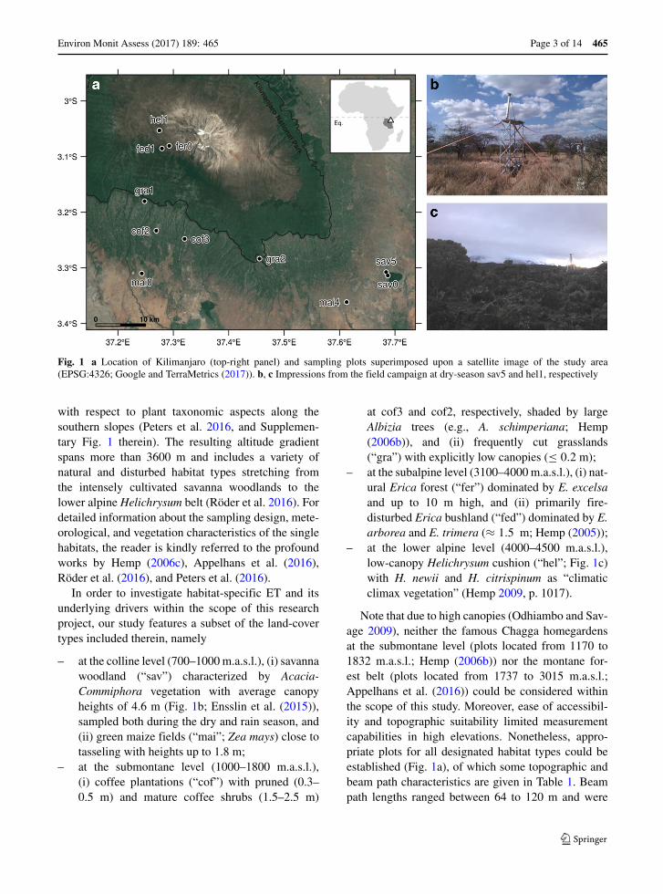
Fig. 1 a Location of Kilimanjaro (top-right panel) and sampling plots superimposed upon a satellite image of the study area(EPSG:4326; Google and TerraMetrics (2017)). b, c Impressions from the field campaign at dry-season sav5 and hel1, respectively

with respect to plant taxonomic aspects along thesouthern slopes (Peters et al. 2016, and Supplemen-tary Fig. 1 therein). The resulting altitude gradientspans more than 3600 m and includes a variety ofnatural and disturbed habitat types stretching fromthe intensely cultivated savanna woodlands to thelower alpine Helichrysum belt (Roder et al. 2016). Fordetailed information about the sampling design, mete-orological, and vegetation characteristics of the singlehabitats, the reader is kindly referred to the profoundworks by Hemp (2006c), Appelhans et al. (2016),Roder et al. (2016), and Peters et al. (2016).

In order to investigate habitat-specific ET and itsunderlying drivers within the scope of this researchproject, our study features a subset of the land-covertypes included therein, namely

– at the colline level (700–1000 m.a.s.l.), (i) savannawoodland (“sav”) characterized by Acacia-Commiphora vegetation with average canopyheights of 4.6 m (Fig. 1b; Ensslin et al. (2015)),sampled both during the dry and rain season, and(ii) green maize fields (“mai”; Zea mays) close totasseling with heights up to 1.8 m;

– at the submontane level (1000–1800 m.a.s.l.),(i) coffee plantations (“cof”) with pruned (0.3–0.5 m) and mature coffee shrubs (1.5–2.5 m)

at cof3 and cof2, respectively, shaded by largeAlbizia trees (e.g., A. schimperiana; Hemp(2006b)), and (ii) frequently cut grasslands(“gra”) with explicitly low canopies (≤ 0.2 m);

– at the subalpine level (3100–4000 m.a.s.l.), (i) nat-ural Erica forest (“fer”) dominated by E. excelsaand up to 10 m high, and (ii) primarily fire-disturbed Erica bushland (“fed”) dominated by E.arborea and E. trimera (≈ 1.5 m; Hemp (2005));

– at the lower alpine level (4000–4500 m.a.s.l.),low-canopy Helichrysum cushion (“hel”; Fig. 1c)with H. newii and H. citrispinum as “climaticclimax vegetation” (Hemp 2009, p. 1017).

Note that due to high canopies (Odhiambo and Sav-age 2009), neither the famous Chagga homegardensat the submontane level (plots located from 1170 to1832 m.a.s.l.; Hemp (2006b)) nor the montane for-est belt (plots located from 1737 to 3015 m.a.s.l.;Appelhans et al. (2016)) could be considered withinthe scope of this study. Moreover, ease of accessibil-ity and topographic suitability limited measurementcapabilities in high elevations. Nonetheless, appro-priate plots for all designated habitat types could beestablished (Fig. 1a), of which some topographic andbeam path characteristics are given in Table 1. Beampath lengths ranged between 64 to 120 m and were

465 Page 4 of 14 Environ Monit Assess (2017) 189: 465

Table 1 Date range,topography and beam pathcharacteristics per plot.‘(d)’ indicates dry-seasonmeasurements

PlotID Date range Topography Beam path

Start (no. of days) Elevation Slope angle Aspect Length Height Inclination

(m.a.s.l.) (◦) (◦) (m) (m) (◦)

fer0 2014329 (6) 3956 17.2 196 100 4 −10.7

hel1 2014335 (5) 3849 9.7 310 120 3 0.8

fed1 2014323 (6) 3498 17.2 264 70 4 −7.8

gra2 2014076 (4) 1754 20.4 94 70 2 −0.5

gra1 2014056 (4) 1742 6.8 146 64 2 4.1

cof2 2014081 (5) 1353 2.8 175 68 5.4 −0.3

cof3 2014070 (3) 1288 18.3 270 103 2.2 4.7

mai0 2014137 (5) 1010 1 177 71 5.3 0.5

mai4 2014133 (5) 962 1.5 273 79 5.3 −1.6

sav0 (d) 2014259 (5) 953 0.8 23 104 5.4 −0.8

sav0 2014125 (5) 953 0.8 23 77 5.4 −0.8

sav5 (d) 2014255 (5) 943 1.2 13 94 5.4 −0.9

sav5 2014129 (5) 943 1.1 13 79 5.3 −0.9

primarily determined by (i) habitat size at low ele-vations, class “sav” excluded and (ii) topographicsuitability at high elevations. Path heights, on the otherhand, were adapted to canopy height and ranged from2 to 5.4 m above ground.

Theoretical and technical background

As regards ground-based remote sensing systems asan alternative to conventional methods such as EC,scintillometer-based techniques (Kite and Droogers2000; Meijninger and de Bruin 2000) have latelyreceived considerable attention regarding their capa-bilities of yielding reliable ET estimates in rathershort time intervals. In this context, the comprehensiveworks by Odhiambo and Savage (2009) and Savage(2009) provide essential information on theoreticalbackground, history, and relevant applications of theSLS method. Briefly, the general principle of scin-tillometry assumes that turbulent fluctuations of airtemperature (Ta), and to a lesser degree, relative airhumidity (rH) induce small-scale fluctuations of therefractive index of air. This, in turn, affects a laserbeam propagating along a given path and hence allowsthe derivation of turbulence-related parameters fromthe resulting intensity fluctuations.

The continuous monitoring of the radiation sig-nal requires a stationary field setup with a transmitterand receiver unit typically positioned 50 to 300 m

apart from each other. Among the advantages associ-ated with the SLS technique (Odhiambo and Savage2009), Nakaya et al. (2007) highlight the represen-tative nature of the path-averaged flux measurementsdue to the larger source area, which makes the tech-nique particularly suitable for small research sites.While requiring no simultaneous wind speed measure-ments in order to derive ET, the SLS results show amore plausible behavior on short time scales as com-pared to EC while maintaining consistent data quality(Thiermann and Grassl 1992).

The herein presented data is derived from a dual-beam SLS of the type SLS40 (Scintec AG, Rot-tenburg, Germany). Complementing factory-certifiedcalibration parameters for wavelength and separationof the laser beam (Van Kesteren et al. 2014), additionalcalibration is carried out in the field through quanti-fying the background signal and crosstalk coefficientsbefore launching the actual measurement. An accom-panying automated weather station (AWS; Scintec(2013a)) records Ta and rH, from which the vaporpressure deficit (VPD) as an important explanatoryvariable of ET in mountainous terrain (Nullet andJuvik 1994) can be calculated, at 1-min intervals. Fur-ther parameters collected by the AWS are air pressure(p), net radiation (Rnet), soil heat flux (S), and rain-fall, among others (Scintec 2013c). Note that windspeed and direction were not collected within thisscope.

Environ Monit Assess (2017) 189: 465 Page 5 of 14 465

Estimation of latent heat flux

Odhiambo and Savage (2009) argue that canopy-related flux terms are negligible for short and opencanopies and, moreover, advection can be left unat-tended when dealing with rather homogeneous sur-faces. Considering the characteristics of the selectedresearch plots (“Study area and sampling design”), theapplication of the shortened energy balance equationto derive the latent heat flux (LE; as a surrogate forET) from

Rnet = LE + H + S (1)

therefore seems justified (Odhiambo and Savage2009). Here, Rnet is net radiation, whereas H and S aresensible and soil heat flux, respectively. It becomesevident that the SLS-based derivation of H allows theestimation of LE given that Rnet and S are available.Note, however, that Eq. 1 cannot be closed entirelywhich, in a more practical sense, means that the resid-ual value (i.e., Rnet – H – S) and the actual LE arenot exactly the same (Tagesson et al. 2015). Despitethis well-known closure issue in boundary-layer mete-orology (e.g., Foken (2008)), Tagesson et al. (2015)underline that averaged daily flux estimates calculatedfrom Eq. 1 may still provide valuable informationwithin the scope of eco-climatological research (e.g.,model validation).

Data processing

The SRun software for automated SLS data retrievalcombines simultaneous optical and meteorologicalrecordings at 1-min intervals (Scintec 2013b), fromwhich hourly ET rates (mm/h) are calculated. Mea-surement gaps introduced during times of power short-age, strong wind and fog add up to 7.2% of all hourlyvalues and are partly refilled using a random forestalgorithm (RF; Breiman (2001)). While filling missingdata introduced by sensor instabilities based on con-comitantly recorded environmental variables is gener-ally considered unproblematic (Goulden et al. 2012),gaps resulting from fog involve a number of unknowns(Dawson 1998) and are hence not recomputed.

Internal validation of the implemented gap-fillingroutine consists of tenfold cross validation (CV) per-formed upon randomly selected training data (75%of all complete records). For a varying number ofsplit variables, the model with the smallest root mean

square error (RMSECV) is used to predict the remain-ing 25% of the complete records. The thus derived ETrates are subsequently compared with the test data bycalculating the test RMSE (RMSET), mean absoluteerror (MAET) and R2

T. The entire procedure is car-ried out ten times for each plot separately to determinethe optimum number of split variables and the meanvalues of all error metrics.

Complementing model validation, the mean vari-able importance of each meteorological input in termsof predicting ET is determined. Briefly, RF-basedvariable importance can be derived through randomlypermuting the values of a given predictor while leav-ing all remaining variables unchanged (Altmann et al.2010). The resulting changes in prediction error (asseen from MAE in regression-based scenarios) serveas a variable-specific measure for the mean decreasein model accuracy (Liaw and Wiener 2002), andtherefore, deploying such an approach is expected toprovide deeper insights for our analysis.

Satellite data

The amount to which vegetation characteristics ofecosystems contribute to ET-elevation relationshipshas been broadly discussed in the literature. In orderto assess potential impacts across multiple land coversin the Kilimanjaro region, our analysis is comple-mented by satellite-borne estimates of the NormalizedDifference Vegetation Index (NDVI) derived fromthe Moderate Resolution Imaging Spectroradiometer(MODIS) aboard the Terra and Aqua satellites. Beinga measure of photosynthetic activity at the Earth’s sur-face, the index distinctly varies between ecosystemsand closely correlates with daytime land surface tem-perature (LST; Maeda and Hurskainen (2014)) andET (Maeda et al. 2011). It is calculated from (Tucker1979)

NDVI = (ρNIR − ρred)/(ρNIR + ρred) (2)

where ρNIR and ρred are reflectances from the near-infrared (841–876 nm) and red MODIS bands (620–670 nm), respectively.

Terra and Aqua-MODIS provide best value com-posites of two selected “Vegetation Indices” (VI),namely Enhanced Vegetation Index (EVI) and NDVI,at a spatial and temporal resolution of 250 mand 16 days, respectively (MOD/MYD13Q1 V006),released with a time lag of 8 days and downloaded

465 Page 6 of 14 Environ Monit Assess (2017) 189: 465

Table 2 Plot-specifictraining and test statistics ofthe random forest-based gapfilling

Plot ID Training Testing

RMSECV R2CV MAET RMSET R2

T

fer0 0.03 ± 0.006 0.96 0.01 ± 0.001 0.03 ± 0 0.96

hel1 0.03 ± 0.005 0.97 0.01 ± 0.001 0.03 ± 0 0.97

fed1 0.07 ± 0.007 0.85 0.03 ± 0.002 0.07 ± 0.001 0.85

gra2 0.03 ± 0.002 0.99 0.01 ± 0.001 0.03 ± 0 0.99

gra1 0.06 ± 0.011 0.93 0.02 ± 0.002 0.05 ± 0.001 0.94

cof2 0.07 ± 0.009 0.94 0.04 ± 0.002 0.06 ± 0.001 0.94

cof3 0.03 ± 0.003 0.99 0.02 ± 0.001 0.03 ± 0 0.99

mai0 0.05 ± 0.005 0.96 0.02 ± 0.001 0.04 ± 0 0.96

mai4 0.04 ± 0.004 0.97 0.02 ± 0.001 0.04 ± 0 0.97

sav0 (d) 0.05 ± 0.003 0.76 0.02 ± 0.001 0.05 ± 0 0.77

sav0 0.07 ± 0.011 0.9 0.03 ± 0.002 0.07 ± 0.001 0.9

sav5 (d) 0.05 ± 0.014 0.58 0.02 ± 0.002 0.06 ± 0.001 0.64

sav5 0.04 ± 0.004 0.85 0.03 ± 0.001 0.04 ± 0 0.86

Included are the root meansquare error (RMSE),coefficient of determination(R2) and, in the case of modeltesting, mean absolute error(MAE). Subscripts “CV” and“T” signify results from modeltraining and testing,respectively, whereas “(d)”indicates dry-seasonmeasurements

from the Land Processes Distributed Active ArchiveCenter (LP DAAC; https://lpdaac.usgs.gov/). Follow-ing two-fold quality control based on the companion“pixel reliability” and “VI quality” layers to retainreliable pixels only, the two datasets are mergedinto a continuous 8-day time series. Finally, a modi-fied Whittaker Smoother (Atzberger and Eilers 2011)is applied for down-weighting remainders of nega-tively biased, low-confidence values in favor of anon-disturbed vegetation signal (Detsch et al. 2016).

Results

Evaluation of ET gap filling

The calculated training and test statistics (Table 2)confirm that the RF-based algorithm used to refillmissing hourly ET rates based on simultaneous mete-orological recordings performs reasonably well. Asfor model training, RMSECV ranges from 0.03 to0.07 mm/h, whereby the associated values of R2

CV(0.58 to 0.99) indicate considerably strong linear rela-tionships. A similar picture is drawn by the test statis-tics, where RMSET and MAET also range from 0.03to 0.07 and 0.01 to 0.04 mm/h, respectively, and R2

Tlies between 0.64 to 0.99.

Complementing the training and test statistics, thecorresponding mean variable importance from internalCV (Fig. 2) indicates that Rnet is the most important

parameter for explaining variations in ET. While p,S, and VPD follow in descending order, Ta and rH—from which VPD is calculated—play only a minorrole. Finally, the relative importance of rainfall is vir-tually zero across all plots, with two minor exceptions(sav5 (d), cof2).

Plo

t ID

sav5

sav5 (d)

sav0

sav0 (d)

mai4

mai0

cof3

cof2

gra1

gra2

fed1

hel1

fer0

Rnet p S VPD Ta rH Rain

0 20 40 60 80 100

Mean variable importance

Fig. 2 Mean relative variable importance per sampling plot(sorted from left to right in descending order of overall impor-tance). Rnet net radiation, p air pressure, S soil heat flux, VPDvapor pressure deficit, Ta air temperature, rH relative humidity.“(d)” indicates dry-season measurements

Environ Monit Assess (2017) 189: 465 Page 7 of 14 465

Elevation profiles

In order to assess the actual influence of the singlemeteorological drivers, further analyses on their short-term interplay with ET are required. As a startingpoint, Fig. 3 depicts the elevation profiles of plot-specific mean daily values of the four most relevantdriving factors.

Rnet lacks a clear altitude gradient as it variesconsiderably between plots even at similar elevationlevels (Fig. 3a). It peaks at the colline maize (mai4,135.7 W/m2) and submontane grassland level (gra1,134.0 W/m2), whereas smaller values become evi-dent from both low (e.g. sav5 (d), 86.0 W/m2) andhigh elevations (e.g. fed1, 65.8 W/m2). Remarkably,dry- and wet-season measurements at sav5 clearly dif-fer, whereas no such seasonal pattern is evident from

sav0. On the other hand, p reveals a much more uni-form distribution as it linearly declines with elevationfrom savanna (sav5, 916.9 hPa) to Helichrysum (hel1,639.6 hPa; Fig. 3b). Rather similar to Rnet, a consid-erably diverse picture is drawn by S, which cannoteasily be subdivided into elevation levels and hencerequires further analysis (Fig. 3c). Interestingly, twoout of three high-elevation plots (hel1, fer0) showpositive flux rates, whereas negative fluxes becomeevident from fed1. At the low-lying sites, the coffeeand grassland habitats as well as sav5 (wet and dry)reveal positive flux rates, whereas sav0 (wet and dry)and maize are characterized by negative or only minorpositive fluxes. Finally, the VPD-elevation relation-ship closely tallies with a strong linear decrease ofTa with elevation (Appelhans et al. 2016, and Fig. 6therein) and reveals highest and lowest deficits at

1000

2000

3000

4000

80 100 120

a) Rnet (W/m2)

700 800 900

b) p (hPa)

−6 −3 0 3 6

c) S (W/m2)

1000

2000

3000

4000

250 500 750

d) VPD (Pa)

1 2 3 4 5

e) ET (mm)

Plot ID

sav5 sav5 (d)

sav0 sav0 (d)

mai4 mai0

cof3 cof2

gra1 gra2

fed1 hel1

fer0

Ele

vatio

n (m

.a.s

.l.)

Fig. 3 Elevation profiles of mean daily a net radiation (Rnet),b air pressure (p), c soil heat flux (S), d vapor pressure deficit(VPD), and e evapotranspiration (ET). In the legend, “(d)”

indicates dry-season measurements, and point shapes and fillcolors signify different land covers and plots per land cover,respectively

465 Page 8 of 14 Environ Monit Assess (2017) 189: 465

dry-season sav5 (858.1 Pa) and hel1 (46.6 Pa), respec-tively (Fig. 3d).

Depicted in Fig. 3e is the determined ET-elevationgradient which vaguely resembles a combinationof the described progression curves of Rnet and S.Accordingly, the highest ET rates are observable atcof2 (5.7 mm/day) that decline both uphill (fed1,2.0 mm/day) and downhill (sav5, 2.5 mm/day). Byfar, the smallest rates become evident during the dryseason in savanna (up to 0.9 mm/day at sav5).

For all variables displayed in Fig. 3a–d, includingrainfall, univariate linear models are fitted to estimatethe degree of variation explained in the observed ET(Table 3). Clearly, Rnet is capable of explaining thebroadest range of variance (R2 0.26 to 0.99), the soleexceptions being dry-season sav5 as well as cof2. Sfollows closely behind and reveals very similar corre-lations as Rnet (R2 0.22 to 0.85), again with the afore-mentioned exceptions. VPD proves to be an importantco-explanatory variable at least at some of the collineand submontane plots (up to R2 = 0.57 at mai0)without following a particular habitat-related pattern.At higher elevations, by contrast, the vapor pressuregradient seems to be of no further relevance. Despitedesignated runner up in terms of RF-based variableimportance, p generally has only little explanatorypower for ET across all elevation levels. Rainfall playsa particular role at dry-season sav5—where the Rnet-based R2 drops to zero—and, to a lesser extent, at cof2

and sav0, while no or only minor showers occurred atthe remaining plots.

The results obtained from multivariate linearregression (Table 3, right column) confirm that,when taking all of the aforementioned variables intoaccount, ET may be reasonably estimated at plot scalein most cases (up to R2 = 1 at gra2). Moreover, whenpooling all data available and building one multivari-ate model for all plots, a comfortably high value ofR2 = 0.71 remains. Still, some deviations downwardspersist at plot scale, which particularly include dry-season sav5 as well as cof2 and sav0, thus pointingtowards additional influence factors that have not beenconsidered so far.

Vegetation characteristics

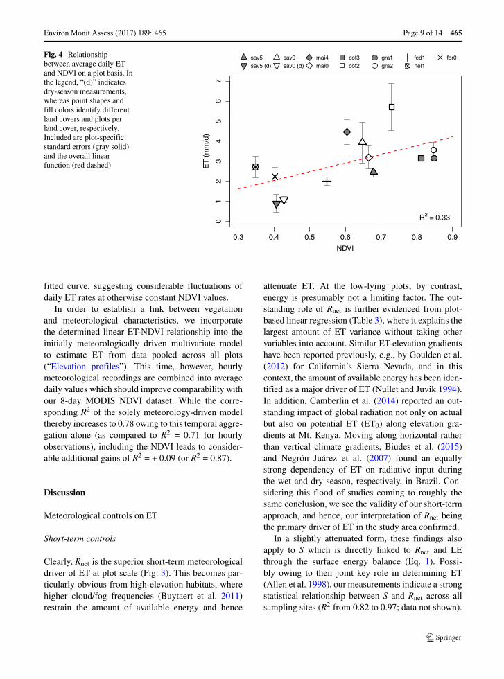
In terms of vegetation characteristics, the highest NDVIvalues occur at the grassland sites (≈ 0.85; Fig. 4)and at cof3 (0.81), which moderately decreasetowards cof2, the two maize fields and the rain-season savanna measurements. With the exceptionof fed1, the upper-mountain habitats and the dry-season savanna measurements reveal explicitlysmaller values between 0.35 and 0.43. Despite theshort measurement periods, the corresponding ET-NDVI relationship proves itself noticeably linear(R2 = 0.33). Plot-specific standard errors therebytend to increase towards the points lying above the

Table 3 Plot-specificcoefficients ofdetermination (R2) derivedfrom univariate andmultivariate linearregression against hourlyET rates. Abbreviations arethe same as in Figs. 2 and 3

PlotID R2 (univariate) R2 (multivariate)

Rnet p S VPD Rain

fer0 0.70 0.09 0.44 0.06 0.10 0.85

hel1 0.88 0.02 0.49 0.03 0.02 0.96

fed1 0.56 0.14 0.26 0.02 0.22 0.89

gra2 0.99 0.03 0.85 0.27 0 1

gra1 0.97 0.11 0.82 0.46 0 0.99

cof2 0.11 0.17 0.10 0.02 0.32 0.63

cof3 0.96 0 0.70 0.16 0 0.98

mai0 0.84 0.03 0.67 0.57 0.03 0.89

mai4 0.75 0 0.68 0.24 0.07 0.87

sav0 (d) 0.83 0.03 0.56 0.14 0 0.88

sav0 0.26 0.02 0.22 0.04 0.29 0.62

sav5 (d) 0.01 0 0 0.04 0.47 0.59

sav5 0.80 0 0.71 0.52 0 0.81

Environ Monit Assess (2017) 189: 465 Page 9 of 14 465

Fig. 4 Relationshipbetween average daily ETand NDVI on a plot basis. Inthe legend, “(d)” indicatesdry-season measurements,whereas point shapes andfill colors identify differentland covers and plots perland cover, respectively.Included are plot-specificstandard errors (gray solid)and the overall linearfunction (red dashed)

sav5sav5 (d)

sav0sav0 (d)

mai4mai0

cof3cof2

gra1gra2

fed1hel1

fer0

0.3 0.4 0.5 0.6 0.7 0.8 0.9

01

23

45

67

NDVI

ET

(m

m/d

)

R2 = 0.33

fitted curve, suggesting considerable fluctuations ofdaily ET rates at otherwise constant NDVI values.

In order to establish a link between vegetationand meteorological characteristics, we incorporatethe determined linear ET-NDVI relationship into theinitially meteorologically driven multivariate modelto estimate ET from data pooled across all plots(“Elevation profiles”). This time, however, hourlymeteorological recordings are combined into averagedaily values which should improve comparability withour 8-day MODIS NDVI dataset. While the corre-sponding R2 of the solely meteorology-driven modelthereby increases to 0.78 owing to this temporal aggre-gation alone (as compared to R2 = 0.71 for hourlyobservations), including the NDVI leads to consider-able additional gains of R2 = + 0.09 (or R2 = 0.87).

Discussion

Meteorological controls on ET

Short-term controls

Clearly, Rnet is the superior short-term meteorologicaldriver of ET at plot scale (Fig. 3). This becomes par-ticularly obvious from high-elevation habitats, wherehigher cloud/fog frequencies (Buytaert et al. 2011)restrain the amount of available energy and hence

attenuate ET. At the low-lying plots, by contrast,energy is presumably not a limiting factor. The out-standing role of Rnet is further evidenced from plot-based linear regression (Table 3), where it explains thelargest amount of ET variance without taking othervariables into account. Similar ET-elevation gradientshave been reported previously, e.g., by Goulden et al.(2012) for California’s Sierra Nevada, and in thiscontext, the amount of available energy has been iden-tified as a major driver of ET (Nullet and Juvik 1994).In addition, Camberlin et al. (2014) reported an out-standing impact of global radiation not only on actualbut also on potential ET (ET0) along elevation gra-dients at Mt. Kenya. Moving along horizontal ratherthan vertical climate gradients, Biudes et al. (2015)and Negron Juarez et al. (2007) found an equallystrong dependency of ET on radiative input duringthe wet and dry season, respectively, in Brazil. Con-sidering this flood of studies coming to roughly thesame conclusion, we see the validity of our short-termapproach, and hence, our interpretation of Rnet beingthe primary driver of ET in the study area confirmed.

In a slightly attenuated form, these findings alsoapply to S which is directly linked to Rnet and LEthrough the surface energy balance (Eq. 1). Possi-bly owing to their joint key role in determining ET(Allen et al. 1998), our measurements indicate a strongstatistical relationship between S and Rnet across allsampling sites (R2 from 0.82 to 0.97; data not shown).

465 Page 10 of 14 Environ Monit Assess (2017) 189: 465

While this is well in agreement with findings fromWest Africa (Kakane 2004), the fact that S gener-ally makes up only a smaller fraction of Rnet (e.g.,Da Rocha et al. (2004)) is likely responsible forthe slightly smaller amounts of explained variance inobserved ET (Table 3). Although the underlying Sto Rnet ratio considerably varies with land-cover typeand season, which has also been one of the key out-comes in Kakane (2004, and references therein), ourresults obtained from univariate regression hence leadus to the conclusion that, complementing Rnet, S is animportant co-explanatory variable for plot-based ETin the region.

In fact, it is only at those plots where precipitationoccurred during our measurements that the relativeimportance of Rnet and S declines (Table 3). In particu-lar, this applies to dry-season sav5 where the impact ofRnet and S practically approaches zero, whereas ET isgoverned almost exclusively by sudden rainfall events.Similar findings were, e.g., reported from semi-aridgrassland and shrubland sites (Nagler et al. 2007),where peak ET rates occurred simultaneous to precip-itation events and, moreover, long-term ET could bebest approximated using rainfall in combination withEVI (R2 = 0.74). Rnet and Ta, on the other hand, wereonly of subordinate importance.

As indicated by previous studies on evaporationprofiles of tropical mountains (e.g., Nullet and Juvik(1994)), linear modeling also suggests that VPD mightbe an essential co-factor impacting ET at least at someof our plots. However, greater uncertainties remain asregards a proper interpretation of this interesting find-ing as higher explanatory power is restricted to someof the lower plots only. At the same time, the amountof explained variance varies considerably between sin-gle land covers and even among plots of the samehabitat type, as seen for example from wet-seasonsavanna sampling. We assume that this behavior can-not entirely be resolved based on the data presentedherein, and therefore, future studies on similar topicsmight provide valuable insights.

Despite indicated otherwise (Fig. 2), we believethat p plays only a minor part in controlling ET. Thisis not only evidenced by plot-based linear regression(Table 3) but also by the fact that the RF procedureindicates a greater significance almost exclusively forwet-season savanna. Here, p typically peaks at aroundlunchtime and drops to a minimum in the late after-noon (data not shown), thus strongly resembling the

diurnal cycle of ET related primarily to Rnet. In con-trast to the remaining habitats, however, no explicitmaximums or minimums are observable during thenight (Hardy et al. 1998), thus agreeing with nocturnalET rates approaching zero.

Possible long-term influences

In addition to short-term controls, we assume the dis-covered ET gradient to be influenced by long-termclimatological factors. Associated with the climategradient are changes in the amount of available mois-ture, with a gradual increase in annual rainfall fromsavanna to the grassland level of roughly + 1300 mm(Appelhans et al. 2016). Of course, these spatial dif-ferences in moisture availability throughout the yearcannot be adequately captured during only a few daysof measurement. However, distinct quantitative devi-ations between dry- and wet-season ET amounts insavanna (Fig. 3e) suggest that water might indeed bea limiting factor at the colline level. This is supportedby the results obtained for maize which is tradition-ally cultivated during the long rains (March to May;Kimaro et al. (2009)) and likewise outweighs ET ratesin dry-season savanna by far. As demonstrated byAppelhans et al. (2016, and Fig. 5 therein), the semi-arid savanna receives most of its annual precipita-tion during the long rains (i.e., wet-season sampling),whereas hardly any rain occurs during the long dryseason from June to September (i.e., dry-season sam-pling). The resulting downregulation of plant stomatalconductance as an adaption of plants to rather dryenvironments (van den Bergh et al. 2013) might con-tribute further to attenuated transpiration rates. On theother hand, intra-annual water availability might notbe such a crucial factor starting from the submontanelevel upwards.

Similar limitations have been reported in quite avariety of eco-climatological studies. Biudes et al.(2015), for instance, found that energy exchange pro-cesses in Brazil savannas were markedly reduced dur-ing the dry season. Moreover, Goulden et al. (2012)reported a rapid ET decline from Sierra Nevada’smontane forest level towards the low-lying savannaareas resulting from less annual rainfall observableeven during the wet season.

In high elevations, by contrast, we assume thatmoisture is not a limiting factor since annual precip-itation amounts do not significantly differ from the

Environ Monit Assess (2017) 189: 465 Page 11 of 14 465

submontane grassland level (Appelhans et al. 2016).Instead, we expect (i) less Rnet resulting from highercloud/fog frequencies (Hemp 2009) and topographicexposure (Nyman et al. 2014) and (ii) reduced VPDresulting from lower Ta to have a dampening effecton ET (van den Bergh et al. 2013). The influence ofexposure becomes particularly evident from the west-exposed and rather steep fed1 (Table 1) that receivesless incident radiation than the south-exposed fer0 orthe flat hel1 plateau.

Vegetation controls on ET

In terms of vegetation properties, we identify a rathergood linear correspondence between ET and NDVI(Fig. 4) documenting that ET in the Kilimanjaroregion is not subject to meteorological influencesalone. Instead, NDVI-based land cover characteristicsseemingly play an important additional role as theyexplain a considerable amount of variation in meandaily ET rates. Accordingly, the highest NDVI val-ues at the submontane grassland/coffee level and themoderate (massive) decline towards lower (higher)situated plots resemble the vaguely hump-shaped ele-vation gradient of ET (Fig. 3e). This is not leastevidenced by the fact that, when adding NDVI tothe already well-performing meteorological model, anadditional boost in explained ET variance (�R2 =+ 0.09) can be achieved. In this context, Nagler et al.(2007) already demonstrated that land cover-specificET could reasonably be estimated as a function ofgreen vegetation derived from EVI (r = 0.80 to 0.94)without deploying meteorological drivers. Moreover,the regional validity of our findings is confirmed byMaeda and Hurskainen (2014) who demonstrated thatland cover properties as seen from the NDVI couldexplain between 26 to 39% of additional spatial vari-ation in daytime LST in the Kilimanjaro region. Asevidenced from the nearby Taita Hills, Kenya (Maedaet al. 2011), LST exerts a substantial impact on poten-tial and actual ET, thus confirming that the hydro-logical cycle is subject to a complex interplay ofmeteorological and land cover-specific factors.

Conclusions

In the study presented herein, we aimed at establishinga short-term ET-elevation gradient along the highly

fragmented southern slopes of Kilimanjaro. Withinthis scope, the major environmental driving factors ofET should be identified to make a step towards assess-ing the consequences of local land-use and global cli-mate change on ecosystem functioning through mod-ifications in the regional-scale water budget. Need-less to say, such ambitious goals—particularly theirgeneralizability—are hard to accomplish with onlya handful of measurement days available. However,we demonstrate that considerable information on thecomplex interplay between ET and its underlyingdriving forces may be deduced even from such explic-itly short-term observations of meteorological andvegetation-related parameters.

As regards the overall elevation profile, ETrevealed a roughly hump-shaped progression curvewhich, in the short term, was strongly linked to the netradiation budget at each elevation level. Topographicinfluences and high cloud/fog frequencies attenuatedET at higher elevations, whereas moisture limitationswere suspected to exert a restraining effect on waterrelease rates at the low-lying savanna woodlands.Consequently, the highest ET amounts occurred atthe submontane coffee/grassland level where neithermoisture nor energy limitations could be identified.

In terms of environmental drivers, we found thatplot-specific ET amounts could be approximated rea-sonably well by multivariate regression involving netradiation, soil heat flux, and to a lesser degree, vaporpressure deficit, air pressure (as a surrogate for ele-vation), and rainfall (R2 0.57 to 1.00). Further gainscould be achieved when including vegetation charac-teristics, resulting in additionally explained variancewhen comparing pooled data multivariate regressionwithout (R2 = 0.71 and 0.78 for hourly and meandaily values, respectively) and with NDVI included(R2 = 0.87).

Having identified the main drivers of ET in the area,future work will presumably aim at testing physicallybased ET modeling approaches to assess the impactsof land-use and climate change on a region-widescale and over longer time periods. In this context,Camberlin et al. (2014), for instance, demonstratedthat seasonal ET0 variability at Mt. Kenya stronglydepended on seasonal fluctuations of moisture avail-ability, air temperature, and global radiation. Consid-ering the explicitly frequent cloud obscuration and thelack of a long-term ground observation network, set-ting up a solely remote sensing-based model on an

465 Page 12 of 14 Environ Monit Assess (2017) 189: 465

appropriate temporal scale remains a challenging yetnot insolvable future goal.

Acknowledgements This study was carried out in the frame-work of the research unit “Kilimanjaro ecosystems under globalchange: Linking biodiversity, biotic interactions and biogeo-chemical ecosystem processes” (KiLi; https://www.kilimanjaro.biozentrum.uni-wuerzburg.de/), and we would like to expressour sincere thanks to the German Research Foundation (DFG)for the provision of funding (funding id Ap 243/1-2, Na 783/5-1, Na 783/5-2). Special thanks go to our diligent Tanzanianfield workers Johannes and Benjamin Silvel, Steve Kuida,and Jimmy Ndyamkama. Finally, we would like to thankour Tanzanian PhD student Ephraim Mwangomo for arrang-ing campaign-related transport and, furthermore, Dr. AndreasHemp for his project-related efforts and his invaluable localknowledge.

Open Access This article is distributed under the terms of theCreative Commons Attribution 4.0 International License (http://creativecommons.org/licenses/by/4.0/), which permits unre-stricted use, distribution, and reproduction in any medium,provided you give appropriate credit to the original author(s)and the source, provide a link to the Creative Commons license,and indicate if changes were made.

References

Afifi, T., Liwenga, E., & Kwezi, L. (2014). Rainfall-inducedcrop failure, food insecurity and out-migration in Same-Kilimanjaro, Tanzania. Climate and Development, 6, 53–60. https://doi.org/10.1080/17565529.2013.826128.

Allen, R.G., Pereira, L.S., Raes, D., & Smith, M. (1998). Cropevapotranspiration—guidelines for computing crop waterrequirements. Irrigation and drainage paper 56, Food andAgriculture Organization of the United Nations, Rome.

Altmann, A., Tolosi, L., Sander, O., & Lengauer, T. (2010).Permutation importance: a corrected feature importancemeasure. Bioinformatics, 26, 1340–1347. https://doi.org/10.1093/bioinformatics/btq134.

Appelhans, T., Mwangomo, E., Otte, I., Detsch, F., Nauss,T., & Hemp, A. (2016). Eco-meteorological character-istics of the southern slopes of Kilimanjaro, Tanzania.International Journal of Climatology, 36, 3245–3258.https://doi.org/10.1002/joc.4552.

Atzberger, C., & Eilers, P.H.C. (2011). Evaluating the effec-tiveness of smoothing algorithms in the absence of groundreference measurements. International Journal of RemoteSensing, 32, 3689–3709. https://doi.org/10.1080/01431161003762405.

Biudes, M.S., Vourlitis, G.L., Machado, N.G., de Arruda,P.H.Z., Neves, G.A.R., Lobo, F.D.A., Neale, C.M.U., &Nogueira, J.D.S. (2015). Patterns of energy exchange fortropical ecosystems across a climate gradient in MatoGrosso, Brazil. Agricultural and Forest Meteorology, 202,112–124. https://doi.org/10.1016/j.agrformet.2014.12.008.

Breiman, L. (2001). Random forests. Machine Learning, 45, 5–32. https://doi.org/10.1023/A:1010933404324.

Buytaert, W., Cuesta-Camacho, F., & Tobon, C. (2011). Poten-tial impacts of climate change on the environmental ser-vices of humid tropical alpine regions. Global Ecology andBiogeography, 20, 19–33. https://doi.org/10.1111/j.1466-8238.2010.00585.x.

Camberlin, P., Boyard-Micheau, J., Philippon, N., Baron, C.,Leclerc, C., & Mwongera, C. (2014). Climatic gradi-ents along the windward slopes of Mount Kenya andtheir implication for crop risks. Part 1: climate variability.International Journal of Climatology, 34, 2136–2152.https://doi.org/10.1002/joc.3427.

Cook, B.I., Smerdon, J.E., Seager, R., & Coats, S. (2014).Global warming and 21st century drying. Climate Dynam-ics, 43, 2607–2627. https://doi.org/10.1007/s00382-014-2075-y.

Da Rocha, H.R., Goulden, M.L., Miller, S.D., Menton, M.C.,Pinto, L.D.V.O., De Freitas, H.C., & Silva Figueira, A.M.E.(2004). Seasonality of water and heat fluxes over a tropi-cal forest in eastern Amazonia. Ecological Applications, 14,S22—S32. https://doi.org/10.1890/02-6001.

Dawson, T.E. (1998). Fog in the California redwood forest:ecosystem inputs and use by plants. Oecologia, 117, 476–485. https://doi.org/10.1007/s004420050683.

DeFries, R., & Eshleman, K.N. (2004). Land-use change andhydrologic processes: a major focus for the future. Hydro-logical Processes, 18, 2183–2186. https://doi.org/10.1002/hyp.5584.

Detsch, F., Otte, I., Appelhans, T., Hemp, A., & Nauss, T.(2016). Seasonal and long-term vegetation dynamics from1-km GIMMS-based NDVI time series at Mt. Kiliman-jaro, Tanzania. Remote Sensing of Environment, 178, 70–83. https://doi.org/10.1016/j.rse.2016.03.007.

Duane, W.J., Pepin, N.C., Losleben, M.L., & Hardy, D.R.(2008). General characteristics of temperature and humid-ity variability on Kilimanjaro, Tanzania. Arctic, Antarctic,and Alpine Research, 40, 323–334. https://doi.org/10.1657/1523-0430(06-127).

Ensslin, A., Rutten, G., Pommer, U., Zimmermann, R., Hemp,A., & Fischer, M. (2015). Effects of elevation and landuse on the biomass of trees, shrubs and herbs at Mount Kil-imanjaro. Ecosphere, 6, 45. https://doi.org/10.1890/ES14-00492.1.

Foken, T. (2008). The energy balance closure problem: anoverview. Ecological Applications, 18, 1351–1367. https://doi.org/10.1890/06-0922.1.

Foley, J.A., DeFries, R., Asner, G.P., Barford, C., Bonan,G., Carpenter, S.R., Chapin, F.S., Coe, M.T., Daily, G.C.,Gibbs, H.K., Helkowski, J.H., Holloway, T., Howard, E.A.,Kucharik, C.J., Monfreda, C., Patz, J.A., Prentice, I.C.,Ramankutty, N., & Snyder, P.K. (2005). Global conse-quences of land use. Science, 309, 570–4. https://doi.org/10.1126/science.1111772.

Glenn, E.P., Nagler, P.L., & Huete, A.R. (2010). Vegetationindex methods for estimating evapotranspiration by remotesensing. Surveys in Geophysics, 31, 531–555. https://doi.org/10.1007/s10712-010-9102-2.

Google and TerraMetrics (2017). Map data. http://maps.googleapis.com/maps/api/staticmap?center=-3.123553240247,37.366348380164&zoom=10&size=640x497&maptype=satellite&format=gif&sensor=false&scale=2. Accessed 25 July2017.

Environ Monit Assess (2017) 189: 465 Page 13 of 14 465

Goulden, M.L., Anderson, R.G., Bales, R.C., Kelly, A.E.,Meadows, M., & Winston, G.C. (2012). Evapotranspirationalong an elevation gradient in California’s Sierra Nevada.Journal of Geophysical Research: Biogeosciences, 117,G03028. https://doi.org/10.1029/2012JG002027.

Hardwick, S.R., Toumi, R., Pfeifer, M., Turner, E.C., Nilus,R., & Ewers, R.M. (2015). The relationship between leafarea index and microclimate in tropical forest and oil palmplantation: forest disturbance drives changes in microcli-mate. Agricultural and Forest Meteorology, 201, 187–195.https://doi.org/10.1016/j.agrformet.2014.11.010.

Hardy, D.R., Vuille, M., Braun, C., Keimig, F., & Bradley,R.S. (1998). Annual and daily meteorological cycles at highaltitude on a tropical mountain. Bulletin of the AmericanMeteorological Society, 79, 1899–1913.

Hemp, A. (2005). Climate change-driven forest fires marginal-ize the impact of ice cap wasting on Kilimanjaro. GlobalChange Biology, 11, 1013–1023. https://doi.org/10.1111/j.1365-2486.2005.00968.x.

Hemp, A. (2006a). Continuum or zonation? Altitudinal gra-dients in the forest vegetation of Mt. Kilimanjaro. PlantEcology, 184, 27–42. https://doi.org/10.1007/s11258-005-9049-4.

Hemp, A. (2006b). The banana forests of Kilimanjaro: biodiver-sity and conservation of the Chagga homegardens. Forestdiversity and management, D. L. Hawksworth and A. T.Bull, eds., Springer, Dordrecht, The Netherlands, 133–155.

Hemp, A. (2006c). Vegetation of Kilimanjaro: hidden endemicsand missing bamboo. African Journal of Ecology, 44, 305–328. https://doi.org/10.1111/j.1365-2028.2006.00679.x.

Hemp, A. (2009). Climate change and its impact on the forestsof Kilimanjaro. African Journal of Ecology, 47, 3–10.https://doi.org/10.1111/j.1365-2028.2008.01043.x.

Jung, M., Reichstein, M., Ciais, P., Seneviratne, S.I., Sheffield,J., Goulden, M.L., Bonan, G., Cescatti, A., Chen, J., deJeu, R., Dolman, A.J., Eugster, W., Gerten, D., Gianelle, D.,Gobron, N., Heinke, J., Kimball, J., Law, B.E., Montagnani,L., Mu, Q., Mueller, B., Oleson, K., Papale, D., Richardson,A.D., Roupsard, O., Running, S., Tomelleri, E., Viovy, N.,Weber, U., Williams, C., Wood, E., Zaehle, S., & Zhang, K.(2010). Recent decline in the global land evapotranspirationtrend due to limited moisture supply. Nature, 467, 951–4.https://doi.org/10.1038/nature09396.

Kakane, V.C.K. (2004). Soil heat flux-net radiation relations forsome surfaces. West African Journal of Applied Ecology, 5,21–29. https://doi.org/10.4314/wajae.v5i1.45599.

Kimaro, A.A., Timmer, V.R., Chamshama, S.A.O., Ngaga,Y.N., & Kimaro, D.A. (2009). Competition between maizeand pigeonpea in semi-arid Tanzania: effect on yields andnutrition of crops. Agriculture, Ecosystems & Environment,134, 115–125. https://doi.org/10.1016/j.agee.2009.06.002.

Kite, G.W., & Droogers, P. (2000). Comparing evapotran-spiration estimates from satellites, hydrological mod-els and field data. Journal of Hydrology, 229, 3–18.https://doi.org/10.1016/S0022-1694(99)00195-X.

Liaw, A., & Wiener, M. (2002). Classification and regressionby randomForest. R News, 2, 18–22.

Maeda, E.E., & Hurskainen, P. (2014). Spatiotemporal charac-terization of land surface temperature in Mount Kilimanjarousing satellite data. Theoretical and Applied Climatology,118, 497–509. https://doi.org/10.1007/s00704-013-1082-y.

Maeda, E.E., Wiberg, D.A., & Pellikka, P.K.E. (2011). Esti-mating reference evapotranspiration using remote sensingand empirical models in a region with limited ground dataavailability in Kenya. Applied Geography, 31, 251–258.https://doi.org/10.1016/j.apgeog.2010.05.011.

Meijninger, W.M.L., & de Bruin, H.A.R. (2000). The sen-sible heat fluxes over irrigated areas in western Turkeydetermined with a large aperture scintillometer. Journalof Hydrology, 229, 42–49. https://doi.org/10.1016/S0022-1694(99)00197-3.

Misana, S.B., Sokoni, C., & Mbonile, M.J. (2012). Land-use/cover changes and their drivers on the slopes ofMount Kilimanjaro, Tanzania. Journal of Geography andRegional Planning, 5, 151–164. https://doi.org/10.5897/JGRP11.050.

Nagler, P.L., Glenn, E.P., Kim, H., Emmerich, W., Scott,R.L., Huxman, T.E., & Huete, A.R. (2007). Relation-ship between evapotranspiration and precipitation pulsesin a semiarid rangeland estimated by moisture flux towersand MODIS vegetation indices. Journal of Arid Envi-ronments, 70, 443–462. https://doi.org/10.1016/j.jaridenv.2006.12.026.

Nakaya, K., Suzuki, C., Kobayashi, T., Ikeda, H., & Yasuike, S.(2007). Spatial averaging effect on local flux measurementusing a displaced-beam small aperture scintillometer abovethe forest canopy. Agricultural and Forest Meteorology,145, 97–109. https://doi.org/10.1016/j.agrformet.2007.04.005.

Negron Juarez, R.I., Hodnett, M.G., Fu, R., Goulden, M.L., &von Randow, C. (2007). Control of dry season evapotranspi-ration over the Amazonian forest as inferred from observa-tions at a southern Amazon forest site. Journal of Climate,20, 2827–2839. https://doi.org/10.1175/JCLI4184.1.

Nullet, D., & Juvik, J.O. (1994). Generalised mountain evap-oration profiles for tropical and subtropical latitudes.Singapore Journal of Tropical Geography, 15, 17–24.https://doi.org/10.1111/j.1467-9493.1994.tb00242.x.

Nyman, P., Sherwin, C.B., Langhans, C., Lane, P.N.J., & Sheri-dan, G.J. (2014). Downscaling regional climate data tocalculate the radiative index of dryness in complex terrain.Australian Meteorological and Oceanographic Journal, 64,109–122.

Odhiambo, G.O., & Ain, A. (2011). Comparison of surfacelayer scintillometer and Eddy covariance footprint and sen-sible heat flux estimates for different wind directions. InIPCBEE (Ed.) 2nd International Conference on Environ-mental Science and Technology, (Vol. 6 pp. V1355–V1360).Singapore: IACSIT Press.

Odhiambo, G.O., & Savage, M.J. (2009). Surface layer scin-tillometry for estimating the sensible heat flux componentof the surface energy balance. South African Journal ofScience, 105, 208–216.

Oettli, P., & Camberlin, P. (2005). Influence of topog-raphy on monthly rainfall distribution over East Africa. Cli-mate Research, 28, 199–212. https://doi.org/10.3354/cr028199.

Peters, M.K., Hemp, A., Appelhans, T., Behler, C., Classen,A., Detsch, F., Ensslin, A., Ferger, S.W., Frederiksen,S.B., Gebert, F., Haas, M., Helbig-Bonitz, M., Hemp, C.,Kindeketa, W.J., Mwangomo, E., Ngereza, C., Otte, I.,Roder, J., Rutten, G., Costa, D.S., Tardanico, J., Zancolli,

465 Page 14 of 14 Environ Monit Assess (2017) 189: 465

G., Deckert, J., Eardley, C.D., Peters, R.S., Rodel, M.-O., Schleuning, M., Ssymank, A., Kakengi, V., Zhang,J., Bohning-Gaese, K., Brandl, R., Kalko, E.K., Kleyer,M., Nauss, T., Tschapka, M., Fischer, M., & Steffan-Dewenter, I. (2016). Predictors of elevational biodiver-sity gradients change from single taxa to the multi-taxa community level. Nature Communications, 7, 13736.https://doi.org/10.1038/ncomms13736.

Roder, J., Detsch, F., Otte, I., Appelhans, T., Nauss, T., Peters,M.K., & Brandl, R. (2016). Heterogeneous patterns ofabundance of epigeic arthropod taxa along a major elevationgradient. Biotropica, 49, 217–228. https://doi.org/10.1111/btp.12403.

Savage, M.J. (2009). Estimation of evaporation using a dual-beam surface layer scintillometer and component energybalance measurements. Agricultural and Forest Meteo-rology, 149, 501–517. https://doi.org/10.1016/j.agrformet.2008.09.012.

Scintec (2013a). Scintec surface layer scintillometer hard-ware manual real-time extension. Scintec AG, Wilhelm-Maybach-Str. 14, 72108 Rottenburg, Germany, version1.06.

Scintec (2013b). Scintec surface layer scintillometer soft-ware manual SRun SLS20/SLS40 SLS20-A/SLS40-ABLS450/BLS900/BLS2000 including SRun real-time sen-sor interface. Scintec AG, Wilhelm-Maybach-Str. 14, 72108Rottenburg, Germany, version 1.12.

Scintec (2013c). Surface layer scintillometer hardware man-ual SLS20/ SLS40 SLS20-A/SLS40-A (including SLSDMIoption). Scintec AG, Wilhelm-Maybach-Str. 14, 72108 Rot-tenburg, Germany, version 1.05.

Tagesson, T., Fensholt, R., Guiro, I., Rasmussen, M.O., Huber,S., Mbow, C., Garcia, M., Horion, S., Sandholt, I., Holm-Rasmussen, B., Gottsche, F.M., Ridler, M.-E., Olen, N.,Olsen, J.L., Ehammer, A., Madsen, M., Olesen, F.S., &Ardo, J. (2015). Ecosystem properties of semiarid savannagrassland in West Africa and its relationship with environ-mental variability. Global Change Biology, 21, 250–264.https://doi.org/10.1111/gcb.12734.

Thiermann, V., & Grassl, H. (1992). The measurementof turbulent surface-layer fluxes by use of bichromaticscintillation. Boundary-Layer Meteorology, 58, 367–389.https://doi.org/10.1007/BF00120238.

Thompson, L.G., Mosley-Thompson, E., Davis, M.E., Hen-derson, K.A., Brecher, H.H., Zagorodnov, V.S., Mashiotta,T.A., Lin, P.-N., Mikhalenko, V.N., Hardy, D.R., & Beer, J.(2002). Kilimanjaro ice core records: evidence of holoceneclimate change in tropical Africa. Science, 298, 589–593.https://doi.org/10.1126/science.1073198.

Torbick, N., Ge, J., & Qi, J. (2009). Changing sur-face conditions at Kilimanjaro indicated from multiscaleimagery. Mountain Research and Development, 29, 5–13.https://doi.org/10.1659/mrd.981.

Tracewski, Ł., Butchart, S.H.M., Donald, P.F., Evans, M.,Fishpool, L.D.C., & Buchanan, G.M. (2016). Patternsof twenty-first century forest loss across a global networkof important sites for biodiversity. Remote Sensing in Ecol-ogy and Conservation, 2, 37–44. https://doi.org/10.1002/rse2.13.

Tucker, C.J. (1979). Red and photographic infrared linearcombinations for monitoring vegetation. Remote Sensingof Environment, 8, 127–150. https://doi.org/10.1016/0034-4257(79)90013-0.

van den Bergh, T., Inauen, N., Hiltbrunner, E., & Korner, C.(2013). Climate and plant cover co-determine the eleva-tional reduction in evapotranspiration in the Swiss Alps.Journal of Hydrology, 500, 75–83. https://doi.org/10.1016/j.jhydrol.2013.07.013.

Van Kesteren, B., Beyrich, F., Hartogensis, O.K., & van denKroonenberg, A.C. (2014). The effect of a new calibra-tion procedure on the measurement accuracy of Scintec’sdisplaced-beam laser scintillometer. Boundary-Layer Mete-orology, 151, 257–271. https://doi.org/10.1007/s10546-013-9891-1.

Weiss, A. (2002). Determination of thermal stratification andturbulence of the atmospheric surface layer over vari-ous types of terrain by optical scintillometry. Zurich: PhDthesis, Swiss Federal Institute of Technology.