A Global Eta Model on Quasi-uniform Gridsgobbert/kali/papers/Zhang_RancicQJ.pdf · A Global Eta Model on Quasi-uniform Grids ... (Arakawa and Lamb 1977), which is a traditional response

Q. J. R. Meteorol. Soc. (2005), 131, pp. 1–999 doi: 10.1256/qj.yy.n

A Global Eta Model on Quasi-uniform Grids

By Hai Zhang1 and Miodrag Rancic2∗

Joint Center for Earth Systems Technology, University of Maryland Baltimore County, USA

Summary

Application of the quasi-uniform grids in global models of the atmosphere is an attempt to increasethe computational efficiency by a more cost effective exploitation of the computing infrastructure. Thispaper describes the development of a global version of NCEP’s regional, step-coordinate, Eta modelon two quasi-uniform girds: cubic and octagonal. The governing equations are expressed in a generalcurvilinear form, so that the cubic and the octagonal version of the model share the same code in spiteof different mapping of the computational domain.

The dynamical core of the derived global Eta model is successfully tested in the benchmark test ofHeld and Suarez. The model with the step-wise formulation of the terrain and full physics is integratedin a series of tests with real data, and the results are compared both with the analysis and the resultsof the regional Eta model.

Keywords: quasi-uniform grids global model Eta

1. Introduction

The objective of this paper is to investigate application of the quasi-uniformgrids for discretization of the governing equations on the sphere, as a solution tothe polar problem of the general circulation models of the atmosphere.

The polar problem is a by-product of the standard longitude-latitude gridand has several aspects. The singular character of geographical poles breaks thepattern of discretization of atmospheric equations on the sphere and complicatespreservation of various integral constraints of the continuous equations withintheir finite-difference approximations. The application of polar Fourier filtering(Arakawa and Lamb 1977), which is a traditional response to the strong increaseof resolution in the latitudinal direction close to poles due to the convergenceof the meridians, is an effective measure for increasing the minimum time-step, but raises many concerns. The most serious of them is a notion that thepolar filtering represents a typical example of an inefficient exploitation of thecomputing infrastructure. The areas around poles are first excessively resolved- wasting memory, and then, through Fourier filtering of the fast modes, theeffect of this resolving is removed - wasting the computing time as well. Thesituation is especially serious in the environment of contemporary distributedmemory computers, where a spatial selectiveness of the polar filtering affects thecomputational balance, causing additional downgrades of the performance.

With the quasi-uniform grids we evade the polar problem, by replacingthe longitude-latitude grid with a mesh of equal (or approximately equal)grid elements. Such a “quasi-uniform” gridding of the sphere may involve theoverlapping grids (e.g., Phillips 1959; Browning et al. 1989) or a continuousmapping (e.g., Sadourny et al. 1968; Williamson 1970). In this paper, we consideronly the quasi-uniform square grids, which have the rectangular base elements,as opposed to the various geodesic grids with the triangular structure of the basicgrid elements (e.g., Ringler and Randall 2002).

Sadourny (1972) suggested first such, a ‘cubic’, grid for the application in thegeneral circulation models of the atmosphere. Sadourny’s cubic grid is derived by

∗ Corresponding author: JCET, Academic IV, 1000 Hilltop Circle, Baltimore, MD 21250, USA.e-mail: [email protected]

c© Royal Meteorological Society, 2005.

1

2 H. ZHANG and M. RANCIC

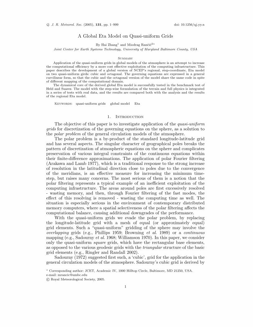
Figure 1. Quasi-uniform grids: cubic (left) and octagonal (right).

a gnomonic projection of the cube to the circumscribed sphere. In the last decadeor so, the distributed memory computers brought once again the application ofthe rectangular quasi-uniform grids in the centre of attention. Rancic et al. (1996)suggested a “conformal” cubic grid as an elegant solution to the problem of anangular discontinuity of the coordinate lines across the edges of the Sadourny’sgnomonic cube. Ronchi et al. (1996) presented an effective overlapping method onthe cubic grid. Purser and Rancic (1997) expanded the set of quasi-uniform gridsby introducing an octagonal grid (or more precisely, the whole series of octagonalgrids with an increasing level of complexity), on which the singular points arearranged along the equator. Within a further refinement of the grid-generationtechnique, Purser and Rancic (1998) enhanced the regularity of the grid-pointdistribution on both cubic and octagonal grids.

The most striking features of these grids are the application of a generalcurvilinear formalism for discretization and the capability to equally distributethe computational load between the processing elements. One can apply exactlythe same code on the cubic grid, all octagonal grids, as well as on any othercontinuous and, with small modifications, overlapping quasi-uniform grids withthe rectangular base elements. Thus, a single unifying model can use any of thesegrids, with an appropriate choice of communications among the processors thatcorresponds to the particular grid topology.

In the last couple of years, several authors accepted quasi-uniform squaregrids as the grid-geometry of choice for the global ocean and/or atmosphericmodels (e.g., McGregor 1996; McGregor and Dix 2001; Tsugawa et al. 2003;Adcroft et al. 2004). In this paper, instead of developing a new global model onthe quasi-uniform grid, we combine the technique of quasi-uniform gridding ofthe sphere with the numerical infrastructure of the regional Eta model, in orderto create a global (or rather, a globalized) version of the Eta model. A globalmodel developed on the quasi-uniform grid has an inclusive design and we referhere to the global Eta model as a Global Eta Framework (GEF). In this paper,the only grids included in this modelling framework are the cubic and the basicoctagonal grid (Figure 1).

The NCEP’s (National Centers for Environmental Prediction) regional Etamodel is a Eulerian grid-point model, whose dynamics is developed followingthe Arakawa principles of integral conservation and of acting on the cause of

A GLOBAL ETA MODEL ON QUASI-UNIFORM GRIDS 3

a numerical problem rather than on its consequences. The early version of themodel has been developed at a ‘Belgrade Numerical School’, in former Yugoslavia,created and led by Dr. Fedor Mesinger and Dr. Zavisa Janjic, the principleauthors of the model. Later developments at NCEP are described, for example,in Mesinger et al. (1988), Janjic (1990; 1994), Black (1994), and Mesinger et al.(2002). The distinguished features of the model are a unique, step-wise treatmentof the lower boundary (Mesinger 1984), and a comprehensive physical package(Janjic 1990; 1994), with inclusion of the land-surface processes (e.g., Chen et al.1997; Ek et al. 2003).

A global version of the regional model, beside a broader spatial coverage, isalso expected to perform better over the domain covered by the regional model.A poor resolution and inadequate treatment of the lateral boundary conditionsare generally considered to be one of the major sources of errors in the limited-area models (e.g., Warner et al. 1997). A global model eliminates the lateralboundary problem and should provide longer and more accurate weather forecastand climate simulations over a specific region of interest.

Section 2 presents the governing equations applied on the quasi-uniformgrids. Section 3 describes numerical methods used to discretize the continuousequations. In section 4, we demonstrate the results of test integrations, whichinclude the Held and Suarez (1994) benchmark test for comparison of dry coresof atmospheric models, and the first experiments with real data and full physics.We provide concluding comments in section 5.

2. Governing equations

The hydrostatic vertical eta (η) coordinate (Mesinger 1984), is defined as

η =p − pT

pS − pTηS , (1)

where

ηS =prf (zS) − pT

prf (0) − pT. (2)

The subscripts S and T stand for the surface and the top of model’satmosphere. prf (z) is a suitably defined reference pressure expressed as a functionof height. zS denotes predefined reference heights of the terrain which may takeonly discrete values. With such a step-wise formulation of the lower boundary,unlike with the customary terrain following used in the σ system of Phillips(1957), the coordinate surfaces remain nearly horizontal, which eliminates errorsof the pressure gradient force close to the steep terrain (Mesinger and Janjic1985). The blocking effect of the step-terrain enforces the component of the flowaround the terrain, which is underestimated in the σ system and is believed tocontribute to a more realistic precipitation forecast (e.g., Mesinger 1996).

The coordinate lines on the cubic and the octagonal grids are strictlyconformal far from the singular points. Close to the singularities, the conformalityconstraint is broken, and the coordinates become curvilinear. The smoothedversions of these grids introduced in Purser and Rancic (1998), have the largerminimum grid distance, but the area where the orthogonality does not applyis also broader. Therefore, in order to describe correctly flow on the quasi-uniform grids, the governing equations need to be expressed in terms of a generalcurvilinear coordinate system.


Let (x, y) define a general curvilinear coordinates on the sphere, and let a1

and a2 be the base vectors of the coordinate transformation in the direction of xand y axis, respectively.

The metric tensor of transformation, G, is defined as

G = Gij = ai · aj , i, j = 1, 2 . (3)

G is the Jacobian of transformation, defined as G = [det(Gij)]12 .

The covariant winds in this system are defined by:

u = V · a1 ,

v = V · a2 . (4)

The contravariant winds are related to the covariant winds via(

u

v

)= G−1

(u

v

). (5)

The relative vorticity is given by

ζ =1G

(∂v

∂x− ∂u

∂y) , (6)

and the kinetic energy by

K =12(uu + vv) . (7)

Further details on application of the general curvilinear coordinate system inthe context of atmospheric primitive equations can be found in Sadourny (1972)and Rancic et al. (1996).

The momentum, the thermodynamic and the continuity equations are re-spectively:

∂u

∂t= (ζ + f)Gv − ∂K

∂x− η

∂u

∂η− ∂Φ

∂x− RTv

p

∂p

∂x+ Fu , (8)

∂v

∂t= −(ζ + f)Gu − ∂K

∂y− η

∂v

∂η− ∂Φ

∂y− RTv

p

∂p

∂y+ Fv , (9)

∂T

∂t= −

(u

∂T

∂x+ v

∂T

∂y

)− η

∂T

∂η+

1cp

RTv

pω +

Q

cp, (10)

∂

∂η

(∂p

∂t

)= − 1

G

[∂

∂x(uGm) +

∂

∂y(vGm)

]− ∂

∂η(ηm) . (11)

The hydrostatic equation is written as:

∂Φ∂η

= −RTv

pm . (12)

Here, the symbols have their usual meanings. The momentum equation iswritten in a vector invariant form, which conveniently encapsulates the curvilinearterms. The mass m is defined as


m =∂p

∂η. (13)

The vertical velocity η is derived from the continuity equation (11)

η∂p

∂η= −∂p

∂t−

∫ η

0

1G

[∂

∂x(uGm) +

∂

∂y(vGm)

]dη . (14)

Similarly, the time tendency of surface pressure is computed by integratingthe horizontal divergence over all layers:

∂pS

∂t= −

∫ ηS

0

1G

[∂

∂x(uGm) +

∂

∂y(vGm)

]dη . (15)

In addition, the transport of a number of atmospheric scalar variables(specific humidity, cloud water, turbulent kinetic energy, etc.) is described by:

∂q

∂t= −

(u

∂q

∂x+ v

∂q

∂y

)− η

∂q

∂η+ Qs , (16)

where Qs are various source and sink terms.

3. Numerical Methods

In this section, we describe the numerical infrastructure used in the GlobalEta Framework. Most of the schemes are simply taken from the regional Etamodel. However, some of the numerical techniques require special modifications,or, in some cases, an adequate replacement, in the general curvilinear system.

(a) Horizontal and vertical arrangement of variablesThe cubic and octagonal quasi-uniform grids (Figure 1) consist respectively,

of 6, and of 14 (or alternatively, 28, if placed diagonally) basic topologicalelements. On the cubic grid, these basic grid elements are identical and coincidewith the faces of the cube. On the octagonal grid, they have equal numberof grid points but cover slightly different areas. More isotropic versions of theoctagonal grid are also available (see Purser and Rancic 1997), but they are notconsidered in this paper. In implementations on the parallel computers, each basictopological element is allocated to its own processor, so that the amount of dataload and computation (at least in the portion of the code which describes theatmospheric dynamics) is equally distributed among processors. Because of thegeneral curvilinear formalism, the only difference in computation on the cubicand the octagonal grid is in definition of communications between the processingelements. The basic grid elements can be further divided into 22, 32, 42, ..., smallerpieces (tiles) depending on the number of available processors and requiredresolution.

The semi-staggered B-grid, following Arakawa notation (Figure 2), is usedfor horizontal staggering of model variables. The B-grid substantially simplifiesindexing in comparison to the E-grid, which is used in the regional Eta model.Because the B- and the E-grid are rotated versions of each other by an angleof 45◦, we are still able to use the efficient E-grid numerical schemes on the B-grid, assuming that the main coordinate lines (x, y) are on the B-grid aligned


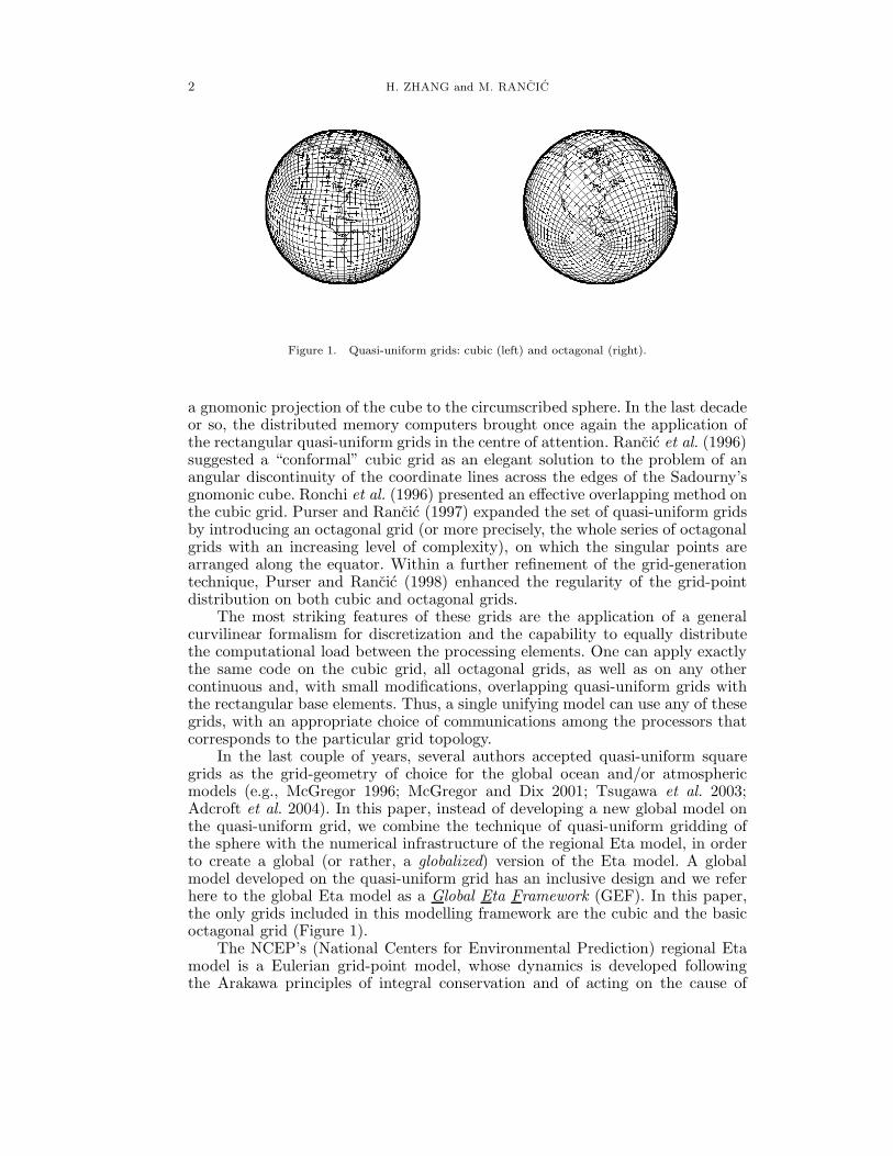
Figure 2. Arakawa B-grid arrangement of variables on a tile of a quasi-uniform grid. T represent scalarpoints and V vector points. If the tile is associated with the corner singularity, then the circled pointsare located in the physically nonexistent, ‘ghost’ space, with values set to 0, and equal T values on each

side from the ghost area.

diagonally. Such a B-grid arrangement with an E-grid definition of the schemeswas introduced in Janjic (1984). The scalar points of the B-grid are placed alongthe boundaries between the tiles. This choice reduces the errors of the pressuregradient force across the boundaries of the faces of the cube and between twoback-to-back octagons that comprise the octagonal grid, as pointed out by Rancicet al. (1996). The values of the variables in the ‘halo’ of a tile are acquired bycommunications from the adjacent tiles. Note that a tile that contains a singularpoint does not have a neighbouring tile in the diagonal direction.

Just as in the regional Eta model, the variables are vertically staggered usinga Lorenz distribution, with the temperature and momentum components definedin the middle of the layers, and the geopotential and the vertical velocity on theinterfaces between the layers.

(b) The dynamicsThe equations describing the dynamics of the hydrostatic atmosphere (mo-

mentum, thermodynamic, continuity, surface pressure and hydrostatic) are dis-cretized in space as:

∂u

∂t=

23Z

x′y′V +

13ZV

yx+ fGv − δxK

x′y′ − δxΦη − πxδxln2 pη − η

x′y′δηu

η

, (17)

∂v

∂t= −2

3Z

x′y′U − 1

3ZU

xy − fGu − δyKx′y′ − δyΦ

η − πyδyln2 pη − η

x′y′δηv

η

,(18)


∂T

∂t= − 1

mG

(UδxT

x + V δyTy)− ηδηT

η

+ 1cpmG

(Uπxδxln2 p

η+ V πyδyln2 p

η) − 1cp

∑ll′=1 Dl′

η, (19)

∂m

∂t= −D − δη(ηmq) , (20)

∂ps

∂t= −

lm∑l=1

Dl , (21)

∆ηΦ = −RTv∆η ln p . (22)

The nonlinear advection terms in the momentum equation are discretizedusing the Janjic (1977) Arakawa-type scheme. A second-order mass and energyconserving spatial differencing is applied for the remaining terms.

The horizontal fluxes, U and V , the relative vorticity, ζ, and the horizontaldivergence, D, are defined respectively as

U = mGx′y′

u ,

V = mGx′y′

v , (23)

ζ =1G

(δxv − δyu) , (24)

D =1G

(δxU + δyV ) . (25)

The potential relative vorticity, Z, is defined as:

Z =ζ

m. (26)

In these expressions, the mass m is defined as the thickness of the eta layers∆ηp, and π is:

π =RTv

2ln pη . (27)

The operators δs and ( )s

represent respectively the two-grid-point finite-difference, and an averaging in the s direction.

A standard technique for suppressing the two-grid-interval noise on the semi-staggered grid (Mesinger 1973; Janjic 1979) is adjusted to the curvilinear frame.This technique consists of a modification of the continuity equation, in which aterm proportional to

−(∇× ·P′ −∇+ · P)

is added to the divergence term. Here, ∇×· and ∇+· are the finite-difference analo-gies of the divergence, and P′ and P are approximations of the pressure gradient


force calculated in the direction of (x′, y′) and (x, y) axes, respectively. Usingthe finite-difference formalism of the general curvilinear system, the modificationterm may be written as

− 1G{[δx′(GPx′) − δy′(GPy′ )] − [δx(GPx) − δy(GPy)]} .

Here, Px′ ,Py′ ,Px and Py are the contravariant components of the pressure gradientforce in the corresponding directions. The contravariant components in thediagonal directions, Px and Py, are:

(Px

Py

)= G−1

(Px

Py

). (28)

In these expressions Px and Py are covariant components of the pressure gradientforce in x and y direction, respectively, defined as

Px = −δxΦη − RTv

2ln pη

x

δxln2 pη

,

Py = −δyΦη − RTv

2ln pη

y

δyln2 pη

. (29)

The contravariant components in the normal directions, Px′ and Py′ , are similarlydefined.

A scalar point located at a corner of the cube or the octagon is surroundedby only three velocity points. In the code, we treat the corner points equally as allother points in the domain, by constructing an artificial ‘ghost’ space at the placeof missing area and by setting the values there to zero. This technique is formallyequivalent to a consistent finite-volume reformulation of the vector operators atthe corner points, and, as stated in Rancic et al. (1996), it enables conservationof the mass, the total energy and the relative vorticity of the general flow (butnot the enstrophy of the non-divergent part of the flow).

The model employs the same explicit time-split differencing for the propa-gation in time as the regional Eta model, with the adjustment time-step beinghalf of that applied to the advection processes. The forward-backward schemeis applied to the gravity-wave terms and the trapezoidal implicit scheme to theCoriolis terms (Mesinger 1977; Janjic 1979). Instead of updating the continuityequation with the forward and the momentum equation with the backward time-differencing scheme, as it is done in the regional Eta model, we reverse theirorder and apply the forward scheme to the momentum and the backward to thecontinuity equation, which we found to be more accurate (Rancic and Zhang2002). The same pattern of time-differencing for the adjustment terms is nowbeing tested within the regional Eta model (e.g., Mesinger et al. 2006).

The multidimensional positive-definite flux corrector scheme of Smolarkiewiczand Grabowski (1990) is applied for the horizontal advection of water vapour andcloud water. Vertical advection is computed using unmodified schemes from theregional Eta model: a piecewise linear upstream scheme for the vertical advectionof humidity and cloud water and the Euler-backward time scheme for the verticaladvection of momentum, temperature, and turbulent kinetic energy.


(c) The physical parameterizationA comprehensive physical package of the regional Eta model is implemented

within the global Eta framework with the minimum modifications.For parameterization of radiation, the model uses the Geophysical Fluid

Dynamics Laboratory (GFDL) scheme (Fels and Schwarzkopf 1975; Lacis andHansen 1974). The surface soil temperature and moisture are predicted using theland-surface scheme described in Chen et al. (1997). The sea surface temperatureis prescribed from NCEP analysis and kept constant during integrations in ourexperiments. The cloud water and ice are treated explicitly as the prognosticvariables using the scheme developed by Zhao and Carr (1997). Just like in theregional Eta model, two schemes for cumulus convection are optionally available:BMJ scheme (Betts 1986; Betts and Miller 1986; Janjic 1990) and Kain-Fritschscheme (Fritsch and Chappell 1980; Kain and Fritsch 1990).

The most notable departures from the physics of the regional Eta model arein the formulation of the horizontal and the vertical diffusion, though the sameexplicit scheme for propagation in time is applied as in the Eta model.

(c).1 Horizontal diffusion

The fourth-order scheme for the lateral diffusion, which is more scale selectivethan the second-order scheme and less affects the larger scales, is applied at theadjustment time-steps for temperature, turbulent kinetic energy and momentumfield.

The diffusion is expressed by a fourth-order Laplacian operator applied in thenormal x′ and y′ directions where the grid distance is minimal. Instead of usingthe general curvilinear system, we approximate the Laplacian operator using aconformal formalism. Technically, we define a new local conformal coordinatesystem (and a new corresponding stencil of grid points) centred at the pointto which we apply the diffusion operator. The values of the variable at thepoints of the local stencil are derived by the high-order interpolations from themodel variables. When applying diffusion to the momentum, we additionallyneed to project winds to the base vectors of the local stencil, and then theresulting Laplacian back to base general curvilinear coordinates, in order to getits covariant components.

This method is designed to cope with the problems that otherwise may arisedue to a combined effect of a strong curvature of the coordinate lines close to thecorners and the application of the fourth-order operator for diffusion, which usesspatially rather distant grid points.

(c).2 Vertical diffusion

Vertical diffusion is applied every 6 adjustment steps to temperature, momentum,water vapour and turbulent kinetic energy. The diffusion coefficients are obtainedfrom the turbulent closure schemes described in Janjic (1990; 1994).

Similarly as in the case of horizontal diffusion, we design an interfacefor transformation between the covariant wind components of the curvilinearsystem and a locally orthogonal system defined at each scalar point separately.Through this interface, the turbulence module from the regional Eta model, whichassumes vertical profiles of the orthogonal wind components, is directly, withoutmodifications, applied to the global Eta model.


4. Results

In this section we present the results of several test integrations of thedeveloped global modelling framework. The dry dynamical core is tested in thetraditional benchmark test of Held and Suarez (1994). The model with full physicsis run in a series of 10-day integrations using real data.

(a) Held-Suarez testThe Held-Suarez test (HS94 hereafter) is commonly used for verification of

the dynamical cores of atmospheric models. In this test, the temperature fieldis relaxed to a prescribed zonally symmetric equilibrium state using a Rayleighdamping at the low-level winds to represent the boundary layer friction.

190190

200

200

210

210 210

220

220

220

230

230 230

230

240

240 240

240

250

250

250

250

260

260

260

260

270

270

270

280

280

290

Latitude

Sig

ma

a

−90 −60 −30 0 30 60 90

0

0.25

0.5

0.75

1

−12

−4

−4−4 −4

4

4

4 44

4

4

4

4

4

4

4

4

12

1212

12

1212

12

12

20

20

20

20

20

20

28

28

28

Latitude

Sig

ma

b

−90 −60 −30 0 30 60 90

0

0.25

0.5

0.75

1

10

10

10

10

10

10

10

10

10

10

20

20

20

20

20

30 30

30

Latitude

Sig

ma

c

−90 −60 −30 0 30 60 90

0

0.25

0.5

0.75

1

2

2

22

2

2

2

2

22

26

6

66

6

66

6

6

6

6

66

10

10

10

10

1010

10

10

10

14

Wavenumber

Latit

ude

d

0 5 10 15−90

−60

−30

0

30

60

90

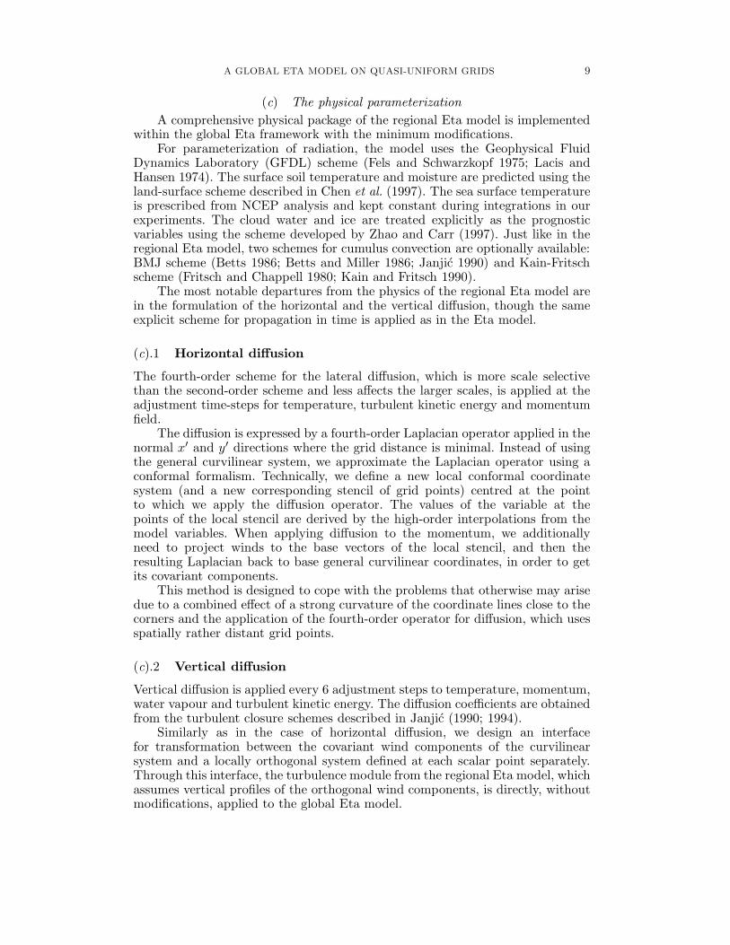
Figure 3. HS94 test of the C42 cubic grid. (a) Zonal mean temperature; (b) Zonal mean wind; (c) Zonalmean zonal wind; (d) Zonal-time mean temperature eddy variance.

Both cubic and octagonal grid models have been integrated in this test withthe fairly similar outcome. Therefore, only the results with the cubic grid will bepresented here for brevity.

The horizontal resolutions of the cubic grid model is set to C42 (42 × 42 × 6grid boxes). Here, the ‘grid box’ is defined as a five-point stencil on the B-gridwith the wind point in the middle and four scalar points at the corners. Thevertical resolution has 20 layers and the pressure at the top of the atmosphereis 25 mb. The model starts integration from an isothermal atmosphere at restand integrates for 1200 days. The statistics are computed for the last 1000 days.The forth-order horizontal diffusion, applied to the temperature and wind field,simulates the physics.

Figures 3 present fields that are obtained in these simulations. These resultsgenerally agree with the solution suggested as the reference in HS94. Figure 3 a


and Figure 3 b show the zonally averaged temperature and the zonally averagedzonal wind, respectively. The midlatitude jets are located at about 40◦ latitudewith the strength of about 30 m/s. The surface maximum westerlies are about4 m/s. The model produces tropical easterlies at all levels. Compared with theresults from HS94, the midlatitude jets are shifted slightly toward equator, andthe surface wind is somewhat weaker.

The eddy temperature variance is shown in Figure 3 c. Two maxima areformed in the midlatitude, one in the lower troposphere and another above thetropopause. The zonal spectrum of the vertically averaged zonal wind varianceis shown in Figure 3 d. The peaks are at the same location as in the HS94, withslightly smaller intensity, and the two midlatitude maxima are at the wavenumbersix rather than at the wavenumber five.

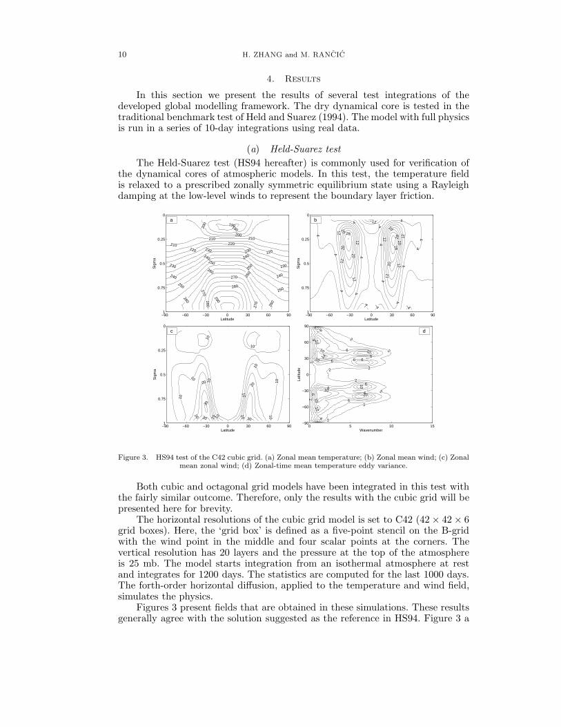
In order to investigate convergence of the derived solution (e.g., Ringler etal. 2000), additional test with the cubic grid at a high resolution (C84, 84x84x6grid boxes) is also performed. The results, shown in Figure 4, are closer to thosesuggested as the reference in HS94. The midlatitude easterlies are located at 45◦,the temperature eddy variance is larger than in C42 experiment, and the twomaxima of midlatitude zonal wind spectra are located at the wavenumber five.

200

200210 210

220 220

220

230

230 230

240

240 240

240

250

250 250

250

260

260

260

260

270

270

270

280

280

280290

290

300

Latitude

Sig

ma

a

−90 −60 −30 0 30 60 90

0

0.25

0.5

0.75

1

−12

−4

−4

−4

−44

44

4

4

4

4

4

4

44

4

12

12

12

12 12

12

12

12

20

20

20

20

20

20

28

28

Latitude

Sig

ma

b

−90 −60 −30 0 30 60 90

0

0.25

0.5

0.75

1

10

10

10

10

10

10

1010

10

10

10

10

20

20

20

20

20

20

30

30 30

30

Latitude

Sig

ma

c

−90 −60 −30 0 30 60 90

0

0.25

0.5

0.75

1

2

2

2

2

2

2

2

22

2

2

2

6

6

66

6

6

6

6

6

6

10

1010

10

10

10 10

1010

10

14

14

14

14

14

14

14

18

Wavenumber

Latit

ude

d

0 5 10 15−90

−60

−30

0

30

60

90

Figure 4. HS94 test of the C84 cubic grid. (a) Zonal mean temperature; (b) Zonal mean wind; (c) Zonalmean zonal wind; (d) Zonal-time mean temperature eddy variance.

(b) Tests with real dataThe developed model is tested in integrations with full physics using real data,

on both the cubic and the octagonal grid. The average horizontal grid distanceused in these tests is shown in Table 1. The corresponding horizontal resolutions,


model grid distance resolution # of grid boxes(km)

C42 219 42 × 42 × 6 10584C100 92 100 × 100 × 6 60000C200 46 200 × 200 × 6 240000O28 215 28 × 28 × 14 10976O68 89 68 × 68 × 14 64736O134 45 134 × 134 × 14 251384

TABLE 1. Grid resolutions in the tests with real data.

expressed as the number of wind points, are also summarized in Table 1. Thenumber of scalar points can be obtained using a general formula:

Ns = τn2 + 2 , (30)

where τ is the number of basic grid elements (6 for cubic and 14 for octagonalgrid), and n is the number of wind grid boxes in each dimension of such anelement.

The vertical resolution has 38 levels, which is a predefined number of levelsin the regional Eta model, structured with a higher density close to the surface.The pressure at the top of the atmosphere is 25 mb.

In these integrations, the primary three-dimensional atmospheric fields, soilmoisture and sea surface temperature are interpolated from the NCEP’s globalanalysis, available at one degree of horizontal resolution. The snow cover in theNorth Hemisphere is determined from the 47-km U.S. Air Force global snowdepth analysis and the 23-km daily NESDIS (National Environmental Satellite,Data and Information Service) Northern Hemisphere snow cover analysis. In theSouthern Hemisphere, the snow cover was determined from NCEP global analysisdata. The initial albedo is derived by interpolation from the seasonal climatevalues.

0 2 4 6 8 100

0.2

0.4

0.6

0.8

1

days

anom

aly

corr

elat

ion

a

C42C100C200

0 2 4 6 8 100

0.2

0.4

0.6

0.8

1

days

anom

aly

corr

elat

ion

b

O28O68O134

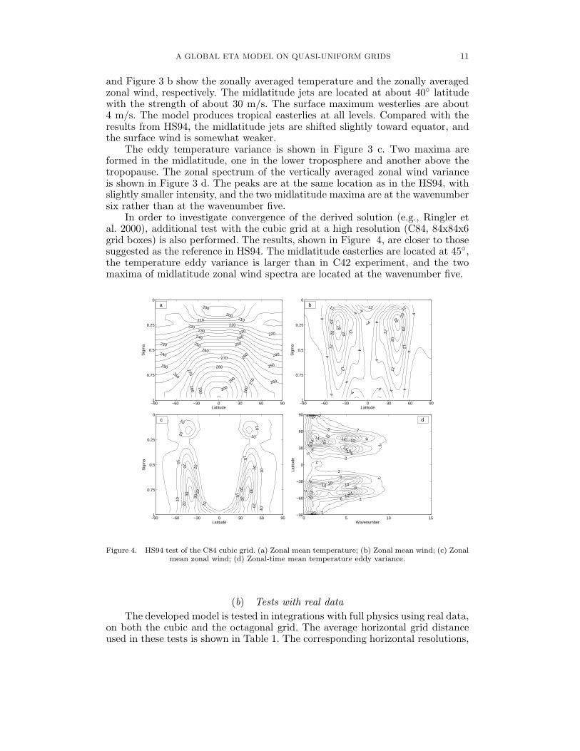
Figure 5. Anomaly correlation of the forecasted 500 mb height with analysis, calculated for the NorthernHemisphere in region of 20◦ − 80◦N : cubic grid (left); octagonal grid (right).

(b).1 Convergence in the tests with real data

Two randomly selected 10-day test cases are run over the whole span of chosenhorizontal resolutions. The initial conditions are taken from 1 February 2005


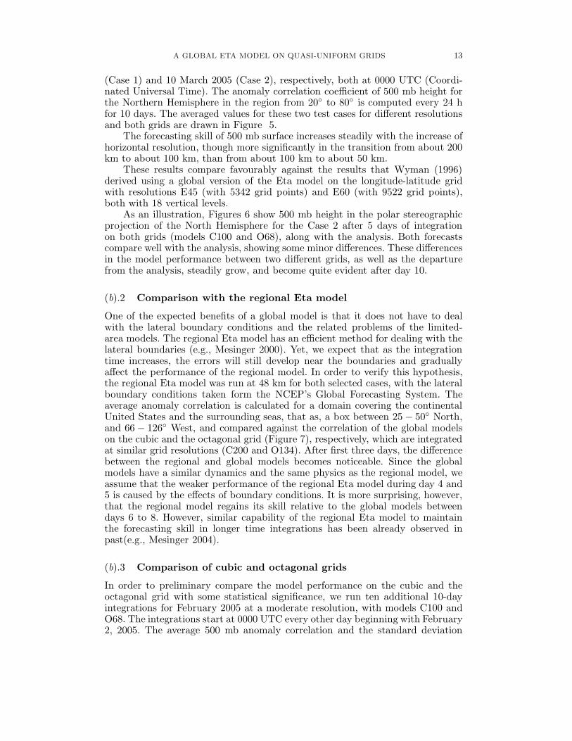
(Case 1) and 10 March 2005 (Case 2), respectively, both at 0000 UTC (Coordi-nated Universal Time). The anomaly correlation coefficient of 500 mb height forthe Northern Hemisphere in the region from 20◦ to 80◦ is computed every 24 hfor 10 days. The averaged values for these two test cases for different resolutionsand both grids are drawn in Figure 5.

The forecasting skill of 500 mb surface increases steadily with the increase ofhorizontal resolution, though more significantly in the transition from about 200km to about 100 km, than from about 100 km to about 50 km.

These results compare favourably against the results that Wyman (1996)derived using a global version of the Eta model on the longitude-latitude gridwith resolutions E45 (with 5342 grid points) and E60 (with 9522 grid points),both with 18 vertical levels.

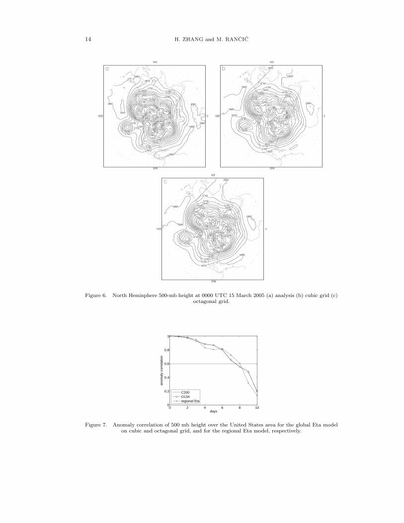
As an illustration, Figures 6 show 500 mb height in the polar stereographicprojection of the North Hemisphere for the Case 2 after 5 days of integrationon both grids (models C100 and O68), along with the analysis. Both forecastscompare well with the analysis, showing some minor differences. These differencesin the model performance between two different grids, as well as the departurefrom the analysis, steadily grow, and become quite evident after day 10.

(b).2 Comparison with the regional Eta model

One of the expected benefits of a global model is that it does not have to dealwith the lateral boundary conditions and the related problems of the limited-area models. The regional Eta model has an efficient method for dealing with thelateral boundaries (e.g., Mesinger 2000). Yet, we expect that as the integrationtime increases, the errors will still develop near the boundaries and graduallyaffect the performance of the regional model. In order to verify this hypothesis,the regional Eta model was run at 48 km for both selected cases, with the lateralboundary conditions taken form the NCEP’s Global Forecasting System. Theaverage anomaly correlation is calculated for a domain covering the continentalUnited States and the surrounding seas, that as, a box between 25 − 50◦ North,and 66 − 126◦ West, and compared against the correlation of the global modelson the cubic and the octagonal grid (Figure 7), respectively, which are integratedat similar grid resolutions (C200 and O134). After first three days, the differencebetween the regional and global models becomes noticeable. Since the globalmodels have a similar dynamics and the same physics as the regional model, weassume that the weaker performance of the regional Eta model during day 4 and5 is caused by the effects of boundary conditions. It is more surprising, however,that the regional model regains its skill relative to the global models betweendays 6 to 8. However, similar capability of the regional Eta model to maintainthe forecasting skill in longer time integrations has been already observed inpast(e.g., Mesinger 2004).

(b).3 Comparison of cubic and octagonal grids

In order to preliminary compare the model performance on the cubic and theoctagonal grid with some statistical significance, we run ten additional 10-dayintegrations for February 2005 at a moderate resolution, with models C100 andO68. The integrations start at 0000 UTC every other day beginning with February2, 2005. The average 500 mb anomaly correlation and the standard deviation


Figure 6. North Hemisphere 500-mb height at 0000 UTC 15 March 2005 (a) analysis (b) cubic grid (c)octagonal grid.

0 2 4 6 8 100

0.2

0.4

0.6

0.8

1

days

anom

aly

corr

elat

ion

C200O134regional Eta

Figure 7. Anomaly correlation of 500 mb height over the United States area for the global Eta modelon cubic and octagonal grid, and for the regional Eta model, respectively.


are presented in (Table 2 and Table 3). The two models have a very similarperformance in these tests, though the model on the cubic grid performs slightlybetter than the model on the octagonal grid.

day 1 2 3 4 5 6 7 8 9 10C100 0.987 0.962 0.921 0.858 0.780 0.697 0.615 0.544 0.479 0.382O68 0.987 0.962 0.921 0.855 0.774 0.689 0.612 0.539 0.464 0.369

TABLE 2. Average 500 mb anomaly correlation in a series of ten additional integrations

day 1 2 3 4 5 6 7 8 9 10C100 0.0019 0.0063 0.015 0.029 0.037 0.048 0.049 0.078 0.12 0.13O68 0.0019 0.0067 0.016 0.031 0.040 0.048 0.053 0.081 0.13 0.14

TABLE 3. Standard deviation of 500 mb anomaly correlation in a series of ten additional integrations

(c) Computational efficiencyThe major motivation for application of the quasi-uniform grids is their clear

potential for improving the computational efficiency. The quasi-uniform gridtopology enables a balanced distribution of the computational load across theprocessors of the massively parallel computer, so that each processor is engagedwith the maximum of its efficiency.

In order to demonstrate this feature of the developed modelling framework,we compare the computational efficiency of dry core of GEF against a model thatexploits the standard longitude-latitude grid. For this comparison, we use a B-gridversion of the atmospheric dynamical core of a Flexible Modeling System (FMS),developed by a GFDL Modeling Team (2004). This is a grid-point model on thelongitude-latitude grid which relies on the application of Fourier polar filtering.The dynamical cores of two models are compared on an IBM 1350 Beowulf Linuxcluster with the high performance capability.

The FMS has horizontal resolution of 144 × 72 × 20, which corresponds to10368 grid-points. GEF is run at horizontal grid configurations C42 and O28(see Table 1 for the corresponding horizontal resolutions). Both models have 20vertical layers.

Table 4 shows the results of the comparison with different number ofprocessors. The time-steps are set at the maximum values capable to maintaina stable integration, which in this case are 360 s, 430 s and 355 s for C42, O28and FMS model, respectively. In spite of application of the Fourier filtering (fromstandard 60 ◦ of latitude toward poles), the time-step of FMS is still smaller thanthat of the global Eta models. The Fourier filtering in these tests takes about20% of total run time of the FMS model. Consequently, the global model onthe quasi-uniform grids, performs more efficiently than the global model on thelongitude-latitude grid.


model time step # of Run time Time spent on(sec) processors per simulated polar filtering per

day (sec) simulated day (sec)C42 360 6 24.0 0C42 360 24 8.0 0O28 430 14 10.1 0FMS 355 6 50.6 10.6FMS 355 14 26.8 6.8FMS 355 24 14.9 3.0

TABLE 4. Comparison of efficiency of GEF and FMS model

5. Conclusions

Quasi-uniform grids eliminate the necessity for polar filtering and generallypromise to improve the computational efficiency. A global version of the regionalEta model has been developed on the quasi-uniform cubic and octagonal grids.

The model dynamics is formulated in terms of general curvilinear system,so that the only difference between the models on the cubic and the octagonalgrid (as well as on any other quasi-uniform grid with the rectangular baseelements) is in formulation of communications between the processing elements.The physical parameterization is taken from the regional Eta model with theminimum modifications. The model can be used both for weather forecasting andclimate simulations, and represents a pioneering prototype for a quasi-uniformexpansion of the regional models of the atmosphere to global coverage.

The dry core of the new model is successfully tested in the Held-Suareztests. The model performance with full physics is verified in a series of 10days integrations at different resolutions. Both grids give similar forecasts of500 mb surface, with the model on the cubic grid being slightly better thanthe model on the octagonal grid, presumably because of the higher resolutionin the extratropical regions. However, note from Table 4 that the octagonalgrid is capable of supporting the larger time-steps than the cubic grid. Overthe United States, the diagnostics of the anomaly correlation of the 500 mbheight is compared to that derived in the corresponding integrations of theregional Eta model. After three days of integration, the global models are clearlybetter as expected, though after day 7 the regional model starts regaining itsrelative skill for a while, among other reasons, most likely because of a somewhatbetter nonlinear momentum advection scheme. Generally, the global model onthe quasi-uniform grids performs better than a global version of the Eta modelon the longitude-latitude grid (Wyman 1996). Dynamical cores of both developedversions of the global Eta model are more efficient than the correspondingdynamical core of atmospheric part of the GFDL’s Forecasting Modeling System.

Admittedly, the method for treatment of the horizontal diffusion in thecurvilinear settings of the global model on the quasi-uniform grids is more timeconsuming than it would be in the orthogonal frame. For example, the fourth-order horizontal diffusion in the global model takes 13.4% out of time spent oncalculation of the dynamical core, and only 10.5% in the regional model.

Work on further testing and improvements of the developed modellingframework is under way.

A more comprehensive testing of various aspects of the model performance,including comparison of the climatology of the cubic, the octagonal and the


longitude-latitude grid versions of the model in the long-term simulations, needsto be done.

One of the strongest features of the regional Eta model is the Janjic (1984)Arakawa type nonlinear advection scheme, as well as its fourth-order counterpart (Rancic 1988), which both successfully constrain the flow of energy in thenonlinear cascading toward (or from) the smallest resolvable scales. We expectthat the implementation of these schemes will further significantly improve theperformance of the presented modelling framework.

Another direction of development is the inclusion of the variable resolutionusing the method of grid stretching (e.g., Fox-Rabinovitz et al. 2001) and applica-tion for the regional climate downscaling. We have recently finished preliminarytesting of the variable resolution concept in the context of quasi-uniform grids(Rancic and Zhang 2006) and we now start working on implementations of gridstretching in the model with full physics.

A version of the regional Eta model with the ‘slope’ (e.g., Adcroft et al. 1997)instead of the ‘step’ approximation of the terrain is now available (Mesingerand Jovic 2004) and incorporation of this upgrade into the global Eta modelframework is also one of the future tasks.

Acknowledgement

The U.S. National Science Foundation (Award Number ATM-0113037) andinternal founds from Joint Center for Earth Systems Technology (JCET) spon-sored the work on this project. We used the Beowulf cluster at the Depart-ment of Mathematics and Statistics of the University of Maryland, BaltimoreCounty (UMBC) for numerical integrations, which was partially supported bythe SCREMS grant DMS-0215373 from the U.S. National Science Foundation,with additional support from UMBC. The authors are grateful to Dr. Ray Hoff,the Director of JCET for his support. Special thanks to Prof. Matthias Gobbertand Prof. Wallace McMillan from UMBC for their help. We also would like toacknowledge the contribution of unknown reviewers of the first version of themanuscript, whose remarks and comments significantly improved the clarity andlevel of presentation.

References

Adcroft, A., Hill C., andMarshall, J.

1997 Representation of topography by shaved cells in a height co-ordinate ocean model. Mon. Weather Rev., 125, 2293-2315

Arakawa, A. and Lamb, V. R. 1977 Computational design of the basic dynamical processes ofthe UCLA general circulation model. in Methods inComputational Physics. 173-265, Academic Press

Betts, A. K. 1986 A new convective adjustment scheme. Part I: Observationaland theoretical basis. Q. J. R. Meteorol. Soc., 112, 677-691

Betts, A. K. and Miller, M. J. 1986 A new convective adjustment scheme. Part II: single columntests using GATE wave, BOMEX and arctic air-massdata sets. Q. J. R. Meteorol. Soc., 112, 693-709

Black, T. L. 1994 The new NMC mesoscale Eta model: Description and fore-cast examples. Weather and Forecasting, 9, 265-278

Browning, G. L., Hack. J. J. andSwarztrauber, P. N.

1989 A comparison of three numerical methods for solving dif-ferential equations on the sphere. Mon. Weather Rev.,117, 1058-1075

Chen, F., Janjic, Z. andMitchell, K.

1997 Impact of atmospheric surface-layer parameterizations in thenew land-surface scheme of the NCEP mesoscale Etamodel. Boundary-Layer Meteorol., 85, 391-421


Ek, M. B., Mitchell, K. E., Lin,Y., Rogers, E., Grunmann,P., Koren, V., Gayno, G.and Tarpley, J. D.

2003 Implementation of Noah land surface model advances inthe National Centers for Environmental Predictionoperational mesoscale Eta model. J. Geophys. Res.108(D22) GCP 12-1 - GCP 12-16

Fels, S. B. and Schwarzkopf, M.D.

1975 The simplified exchange approximation: a new method forradiative transfer calculations. J. Atmos. Sci., 32, 1475-1488

Fox-Rabinovitz, M. S., Takacs,L. L., Govindaraju, R. C.and Suarez, M.

2001 A variable resolution stretched-grid general circulationmodel: regional climate simulation. Mon. Weather Rev.,129, 453-469

Fritsch, J. M. and Chappell, C.F.

1980 Numerical prediction of convectively driven mesoscale pres-sure systems. Part I: convective parameterization. J.Atmos. Sci., 37, 1722-1733

GFDL Global AtmosphericModel Development Team(list of 33 authors)

2004 The new GFDL global atmospheric and land model. AM2-LM2: Evaluation with prescribed SST simulation. J.Climate, 17, 4641-4673

Held, I. and Suarez, M. 1984 A proposal for intercomparison of the dynamical coresof atmospheric general circulation models. Bull. Am.Meteorol. Soc.,73, 1825-1830.

Janjic, Z. I. 1977 Pressure gradient force and advection scheme used for fore-casting with steep and small scale topography. Beitr.Phys. Atmos., 50, 186-199

1979 Forward-backward scheme modified to prevent two-grid-interval noise and its application in sigma coordinatemodels. Beitr. Phys. Atmos., 52, 69-84

1984 Nonlinear advection schemes and energy cascade on semi-staggered grids. Mon. Weather Rev., 112, 12341245

1990 The step-mountain coordinate: physical package. Mon.Weather Rev., 118, 1429-1443

1994 The step-mountain eta coordinate model: Further develop-ments of the convection, viscous sublayer, and turbu-lence closure schemes. Mon. Weather Rev., 122, 927-945

Kain, J. and Fritsch, J. M. 1990 A one-dimensional entraining/detraining plume model andits application in convective parameterization. J.Atmos. Sci., 47, 2784-2802

Lacis, A. A. and Hansen, J. E. 1974 A parameterization for the absorption of solar radiation inthe earth’s atmosphere. J. Atmos. Sci., 31, 118-133

McGregor, J. L. 1996 Semi-Lagrangian advection on conformal-cubic grids. Mon.Weather Rev., 124, 1311-1322

McGregor, J.L. and Dix, M. R. 2001 The CSIRO conformal-cubic atmospheric GCM. In IUTAMSymposium on Advances in Mathematical Modelling ofAtmosphere and Ocean Dynamics, Ed. P. F. Hodnett,Kluwer, Dordrecht, 197-202

Mesinger, F. 1973 A method for construction of second-order accuracy differ-ence schemes permitting no false two-grid-interval wavein the height field. Tellus, 25, 444-458

1977 Forward-backward scheme, and its use in a limited areamodel. Beitr. Phys. Atmos., 50, 200-210

1984 A blocking technique for representation of mountains inatmospheric models. Riv. Meteor. Aeronautica., 44,195-202

1996 Improvements in quantitative precipitation forecasts withthe Eta regional model at the National Centers forEnvironmental Prediction. The 48-km upgrade. Bull.Am. Meteorol. Soc., 77, 2637-2649

2000 Numerical Methods: The Arakawa approach, horizontal grid,global and limited-area modeling. In: General Circu-lation Model Development. Past, Present and Future.Academic Press, Ed. D. A. Randall, 373-419

2004 Dynamical core design: A neglected thrust toward increasingNWP skill several days ahead. In: The First THORPEXInternational Science Symposium. Montreal, Canada,6-10 December 2004


Mesinger, F., and Janjic, Z. I. 1985 Problems and numerical methods of the incorporation ofmountains in atmospheric models. In Large-scale Com-putations in Fluid Mechnaics, Part 2, Lect. Appl. Math.,22, 81-120

Mesinger, F., Janjic, Z. I.,Nickovic, S., Gavrilov, D.and Deaven, D. G.

1988 The step mountain coordinate: Model description and per-formance for cases of Alpine Cyclogenesis and for a caseof an Appalachian redevelopment. Mon. Weather Rev.,116, 1493-1518

Mesinger, F., Black, T., Brill,K., Chuang, H.-Y., DiMego,G. and Rogers, E.

2002 A decade+ of the Eta performance, including that beyondtwo days: Any lessons for the road ahead? Preprints,19th Conf. on Weather Analysis and Forecasting/15thConf. on Numerical Weather Prediction, San Antonio,TX, Am. Meteorol. Soc., 387-390

Mesinger, F. and Jovic, D. 2004 Vertical coordinate, QPF, and resolution. The 2004Workshop on the Solution of Partial DifferentialEquations on the Sphere, Frontier Res. Center forGlobal Change (FRCGC), Yokohama, Japan, 20-23July 2004. ppt in CD-ROM, Vol. 2. Available also athttp://www.jamstec.go.jp/frcgc/eng/workshop/pde2004/agenda.html.

Mesinger, F., Rancic, M., Jovic,D., Zhang. H., and Popovic,J.

2006 Forward-backward scheme modified to suppress lattice sep-aration and impact of the order of execution. GeneralAssembly of the European Geosciences Union, Vienna,Austria, Vienna, Austria, 02 - 07 April 2006, EGU06-A-10164.

Phillips, N. A. 1957 A coordinate system having some special advantages fornumerical forecasting. J. Meteorol., 14, 184-185

1959 Numerical integration of the primitive equations on thehemisphere. Mon. Weather Rev., 87, 333-345

Purser, R.J. and Rancic, M. 1997 Conformal octagon: an attractive framework for global mod-els offering quasi-uniform regional enhancement of res-olution. Meteorol. Atmos. Phys., 62, 33-48

1998 Smooth quasi-homogeneous gridding of the sphere. Q. J. R.Meteorol. Soc., 124, 637-647

Rancic, M., 1988 Fourth-order horizontal advection schemes on the semi-staggered grid. Mon. Weather Rev., 116, 1274-1288

Rancic, M. and Nickovic, S. 1988 Numerical testing of E-grid horizontal advection schemes onthe hemisphere. Beitr. Phys. Atmos., 61, 265-274

Rancic, M., Purser, R.J. andMesinger, F.

1996 A global shallow-water model using an expanded sphericalcube: gnomonic versus conformal coordinates. Q. J. R.Meteorol. Soc., 122, 959-982

Rancic, M., and Zhang, H. 2002 A framework for globalization of regional atmospheric mod-els: Dry core and quasi-uniform grids. In: Preprints,15th Conference of Numerical Weather Prediction. SanAntonio, Texas, 12-16 August 2002. American Meteoro-logical Society. 4B6

2006 Variable resolution on quasi-uniform grids: Linear ad-vection experiments. Meteorol. Atmos. Phys., DOI10.1007/s00703-005-0165-4

Ringler, T., Heiks, R. P.,Randall, D.

2000 Modeling the atmospheric general circulation using a spheri-cal geodesic grid: A new class of dynamical cores. Mon.Weather Rev., 128, 2471-2489

Ringler, T. and Randall, D. 2002 Potential enstrophy and energy conserving numerical schemefor solution of the shallow water equations on a geodesicgrid. Mon. Weather Rev., 130, 1397-1410

Ronchi, C., Iaccono, R.,Paolucci, P. S.

1996 The ‘cubed sphere’: A new method for the solution of partialdifferential equations in spherical geometry. J. Comput.Phys., 124, 93-114

Sadourny, R. 1972 Conservative finite-differencing approximations of the prim-itive equations on quasi-uniform spherical grids. Mon.Weather Rev., 22, 1107-1115

Sadourny, R., Arakawa, A. andMintz, Y.

1968 Integration of the nondivergent barotropic vorticity equationwith an icosahedral-hexagonal grid for the sphere. Mon.Weather Rev., 96, 351-356

Smolarkiewicz, P. K. andGrabowski, W. W.

1990 The multidimensional positive definite advection transportalgorithm: nonoscillatory option. J. Comput. Phys., 86,355-375


Tsugawa, M., Tanaka, Y.,Mimura, Y., and Sakashita,M.

2003 Approach to a high-resolution parallel OGCM for the EarthSimulator. The 5th International Workshop on NextGeneration Climate Models for Advanced High Perfor-mance Computing Facilities, March 3-5, 2003 at INGVin Rome, Italy

Warner, T. T., Peterson, R. A.and Treadon, R. T.

1997 A tutorial on lateral boundary conditions as a basic andpotentially serious limitation to regional numericalweather prediction. Bull. Am. Meteorol. Soc., 78, 2599-2617

Wayman, B. L. 1996 A step-mountain coordinate general circulation mode: De-scription and validation of medium-range forecasts.Mon. Weather Rev., 124, 102-121

Williamson, D. L. 1970 Integration of the primitive barotropic model over a sphericalgeodesic grid. Mon. Weather Rev., 98, 512-520

Zhao, Q. and Carr, F. H. 1997 A prognostic cloud scheme for operational NWP models.Mon. Weather Rev., 125, 1931-1953

Documents

A Global Eta Model on Quasi-uniform Gridsgobbert/kali/papers/Zhang_RancicQJ.pdf · A Global Eta Model on Quasi-uniform Grids ... (Arakawa and Lamb 1977), which is a traditional response