Embed Size (px)
Citation preview


A helical tube of virus head protein.
The protein subunits can be seen clearly in some places but not others.
Although we see some regularities, they are not everywhere.
Is this simply a bad image?
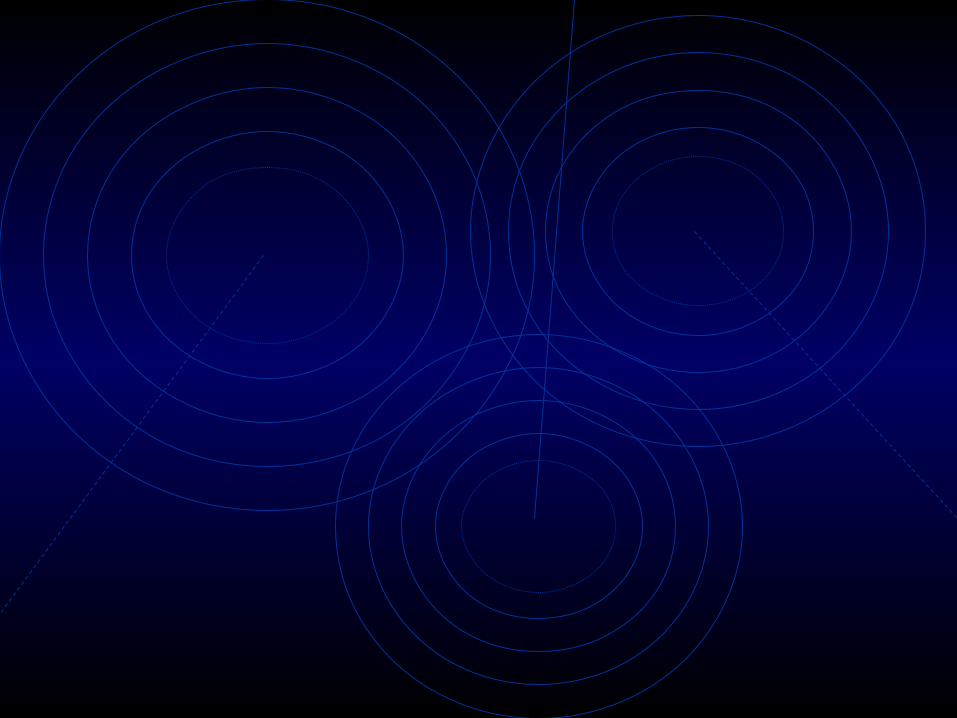
Photographic image superposition (averaging) by Roy Markham.The image is shifted and added to the original.
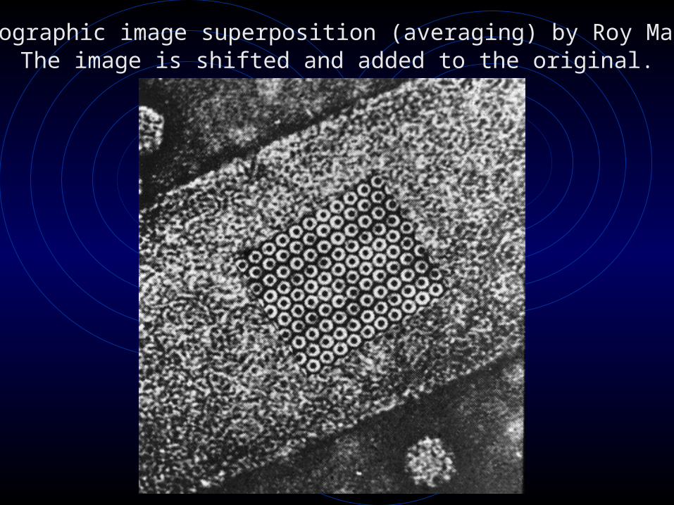
Superimposed images using Adobe Photoshop.
I used Markham’s lattice to determine how much to shift by.
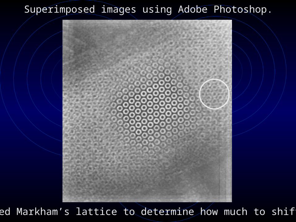
How would I figure out the distance and direction to shift if there weren’t a guide?
1. I could guess and pick the answer (image) that I liked best.
2. I could try all possible shifts and pick out the image with the strongest features (measured objectively rather than subjectively).
The Fourier transform carries out the essence of method 2.

EM of catalase
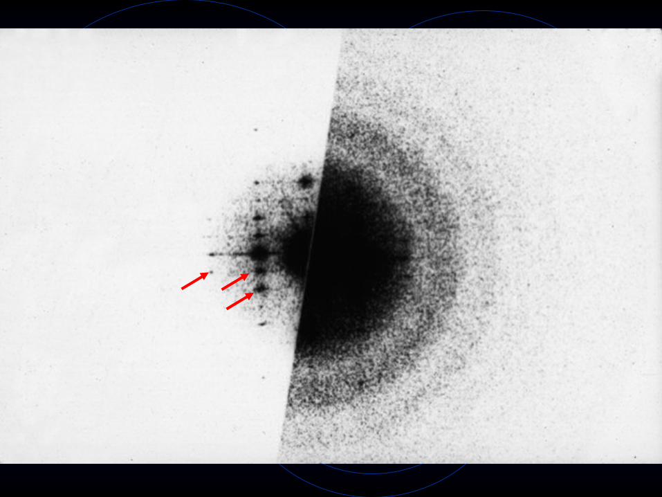
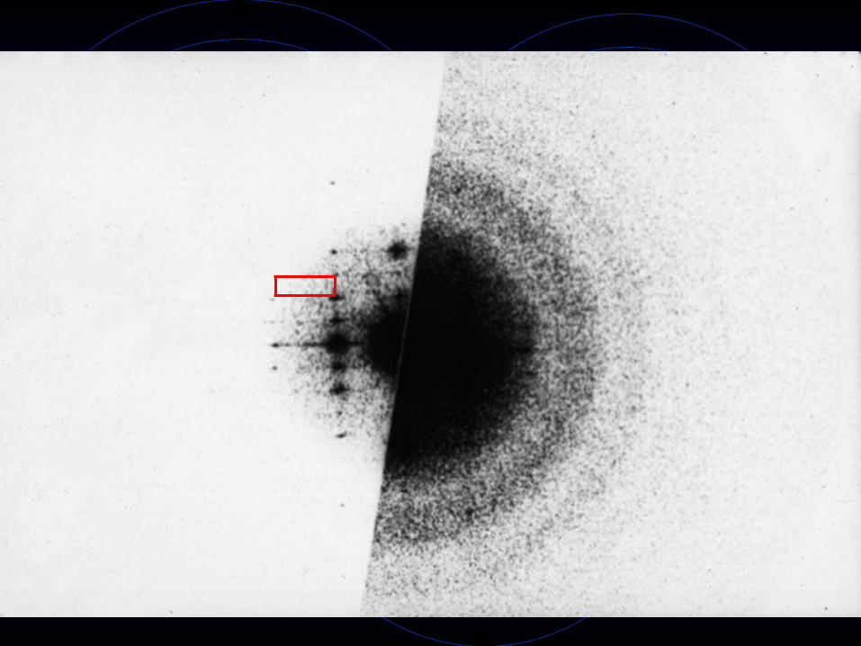
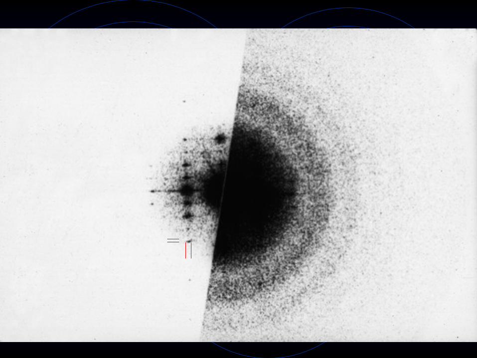
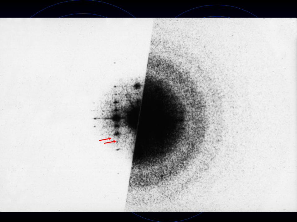
Optical diffraction pattern weak and strong exposure.
(Erikson and Klug, 1971)

Bacterial rhodopsin in glucose Fourier transform of image.

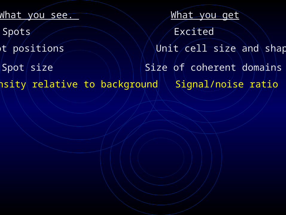
What you see. What you get
Spots Excited

What you see. What you get
Spots Excited
Spot positions Unit cell size and shape

What you see. What you get
Spots Excited
Spot positions Unit cell size and shape
Spot size Size of coherent domains
What you see. What you get
Spots Excited
Spot positions Unit cell size and shape
Spot size Size of coherent domains
Intensity relative to background Signal/noise ratio
What you see. What you get
Spots Excited
Spot positions Unit cell size and shape
Spot size Size of coherent domains
Intensity relative to background Signal/noise ratio
Distance to farthest spot Resolution

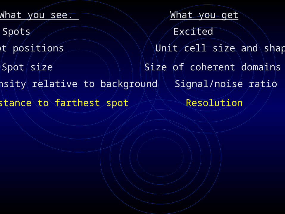
What you see. What you get
Spots Excited
Spot positions Unit cell size and shape
Spot size Size of coherent domains
Intensity relative to background Signal/noise ratio
Distance to farthest spot Resolution
Amplitude and phases of spots Structure of molecules


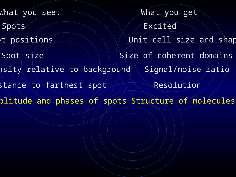
What you see. What you get
Spots Excited
Spot positions Unit cell size and shape
Spot size Size of coherent domains
Intensity relative to background Signal/noise ratio
Distance to farthest spot Resolution
Amplitude and phases of spots Structure of molecules
Positions of Thon rings Amount of defocus


What you see. What you get
Spots Excited
Spot positions Unit cell size and shape
Spot size Size of coherent domains
Intensity relative to background Signal/noise ratio
Distance to farthest spot Resolution
Amplitude and phases of spots Structure of molecules
Positions of Thon rings Amount of defocus
Ellipticity of Thon rings Amount of astigmatism
Asymmetric intensity of Thon rings Amount of instability
Direction of asymmetry Direction of instability

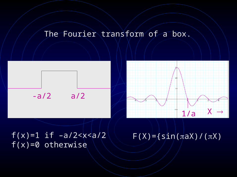
F(X)={sin(aX)/(X)
-a/2 a/2
1/a
The Fourier transform of a box.
f(x)=1 if –a/2<x<a/2f(x)=0 otherwise
X

Fourier transform of a constant.
f(x)=1 F(X)= (X)
0 X x
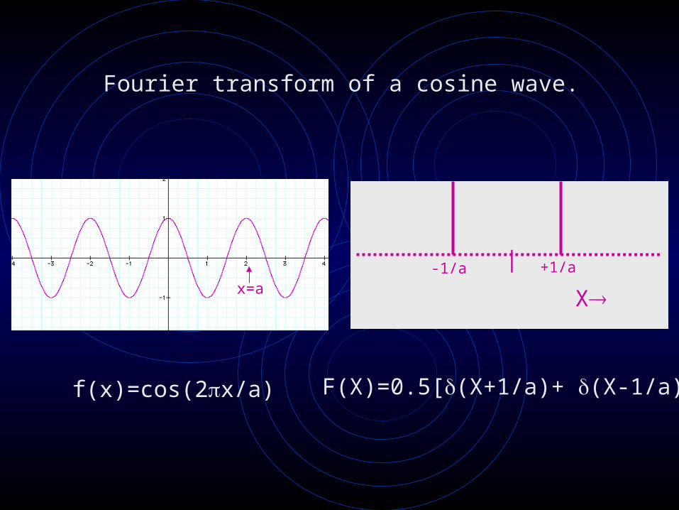
x=a
Fourier transform of a cosine wave.
f(x)=cos(2x/a)
-1/a +1/a
F(X)=0.5[(X+1/a)+ (X-1/a)]
|
X
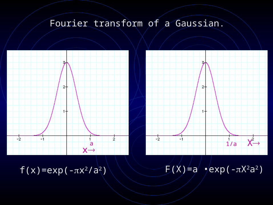
Fourier transform of a Gaussian.
f(x)=exp(-x2/a2) F(X)=a •exp(-X2a2)
a 1/a Xx
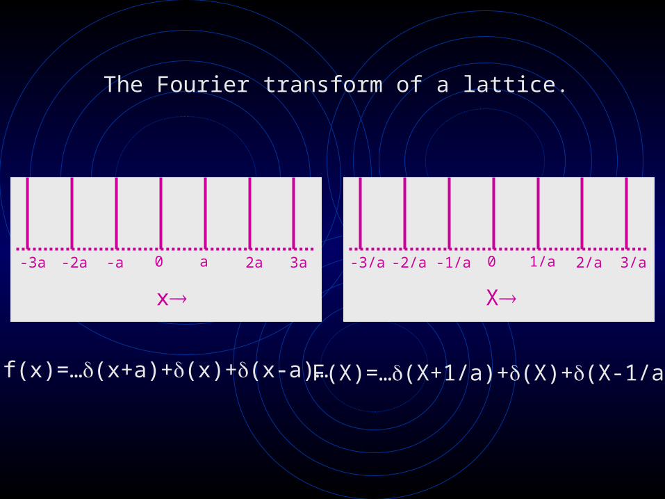
-a a0-2a-3a 2a 3a
The Fourier transform of a lattice.
f(x)=…(x+a)+(x)+(x-a)…
-1/a 1/a0-2/a-3/a 2/a 3/a
F(X)=…(X+1/a)+(X)+(X-1/a)…
x X

In 2D the transform of a row of periodically placed points is a set of lines. This set of lines is perpendicular to the line joining the points.
d
f(x)
1/d
F(X)
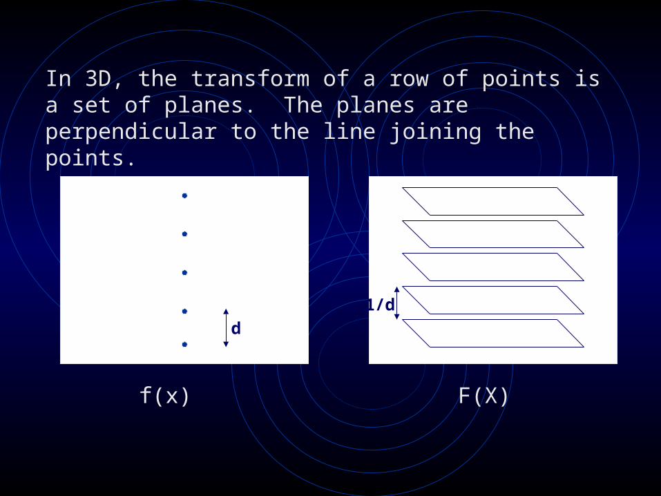
In 3D, the transform of a row of points is a set of planes. The planes are perpendicular to the line joining the points.
d
f(x)
1/d
F(X)

In 3D, the transform of a plane of evenly spaced lines is a plane of evenly placed lines. These lines in real space are perpendicular to the plane containing the lines in reciprocal space (and vice versa).
d
f(x)
1/d
F(X)


If F(X)=FT[f(x)], then f(x)=IFT[F(X)]
where FT=Fourier transform & IFT=Inverse Fourier transform.
USE: If you can obtain the Fourier transform, F(X), of an object, you can regenerate the object itself.
This is the basis of x-ray crystallography and some 3D reconstruction algorithms.
1. Inverse Fourier transform:
FT[ a•f(x) ] = a•F(X)
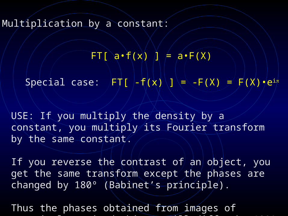
2. Multiplication by a constant:
Special case: FT[ -f(x) ] = -F(X) = F(X)•ei
USE: If you multiply the density by a constant, you multiply its Fourier transform by the same constant.
If you reverse the contrast of an object, you get the same transform except the phases are changed by 180º (Babinet’s principle).
Thus the phases obtained from images of negatively stained objects will differ by 180º from those of an ice-embedded object.
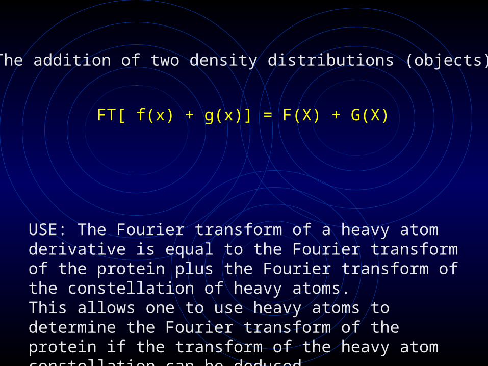
3. The addition of two density distributions (objects):
FT[ f(x) + g(x)] = F(X) + G(X)
USE: The Fourier transform of a heavy atom derivative is equal to the Fourier transform of the protein plus the Fourier transform of the constellation of heavy atoms. This allows one to use heavy atoms to determine the Fourier transform of the protein if the transform of the heavy atom constellation can be deduced.
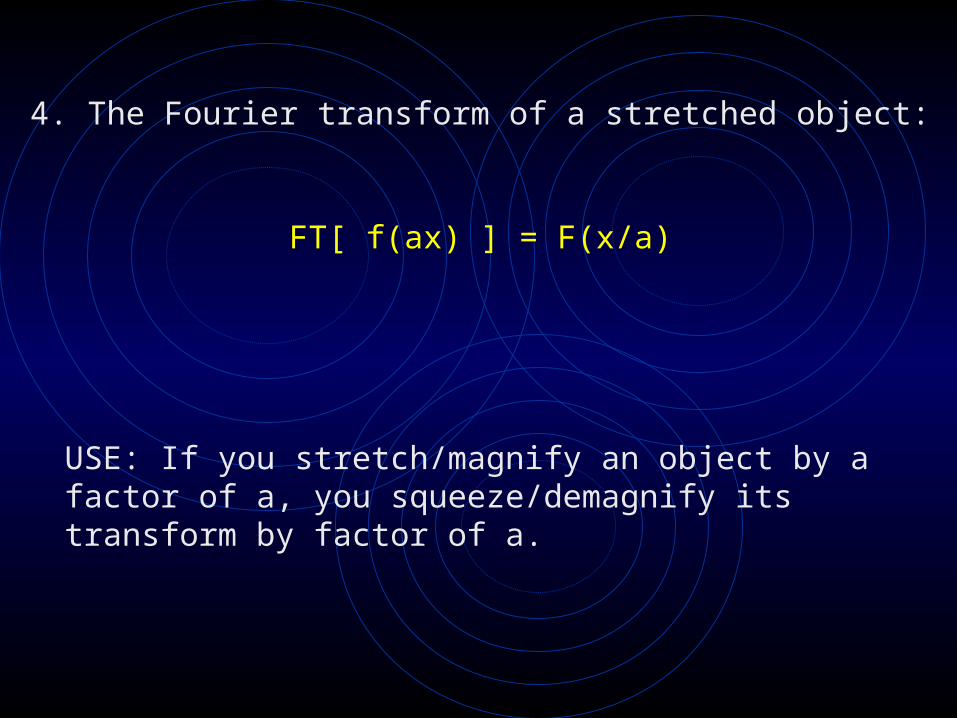
4. The Fourier transform of a stretched object:
FT[ f(ax) ] = F(x/a)
USE: If you stretch/magnify an object by a factor of a, you squeeze/demagnify its transform by factor of a.
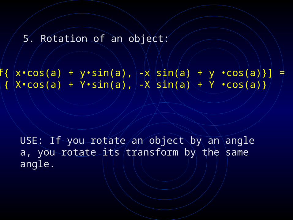
5. Rotation of an object:
FT[ f{ x•cos(a) + y•sin(a), -x sin(a) + y •cos(a)}] = F { X•cos(a) + Y•sin(a), -X sin(a) + Y •cos(a)}
USE: If you rotate an object by an angle a, you rotate its transform by the same angle.

6. Fourier transform of a shifted object:
FT[ f(x-a) ] = F(X)•eiaX
USE: If you shift an object by +a, you leave the amplitudes of its transform unchanged but its phases are increased by aX radians = 180ºaX degrees.
The electron diffraction pattern is not sensitive to movement of the specimen since the intensities do not depend on phases. Vibration of the specimen does not affect the electron diffraction patterns as it does the images.

7. The section/projection theorem:
FT[ f(x,y,z)dx ] = F(0,Y,Z)
USE: The Fourier transform of a projection of a 3D object is equal to a central section of the 3D Fourier transform of the object.
An electron micrograph is a projection of a 3D object.
Its transform provides one slice of the 3D transform of the 3D object.
By combining the transforms of different views, one builds up the 3D transform section by section.
One then uses the IFT to convert the 3D transform into a 3D image.
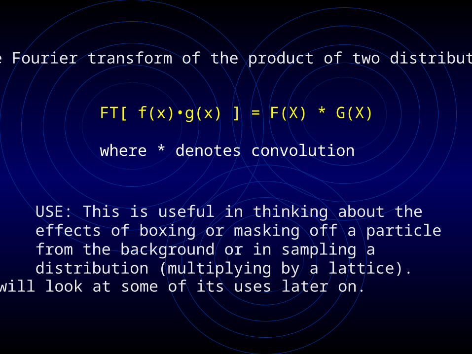
8. The Fourier transform of the product of two distributions:
FT[ f(x)•g(x) ] = F(X) * G(X)
where * denotes convolution
USE: This is useful in thinking about the effects of boxing or masking off a particle from the background or in sampling a distribution (multiplying by a lattice).
We will look at some of its uses later on.
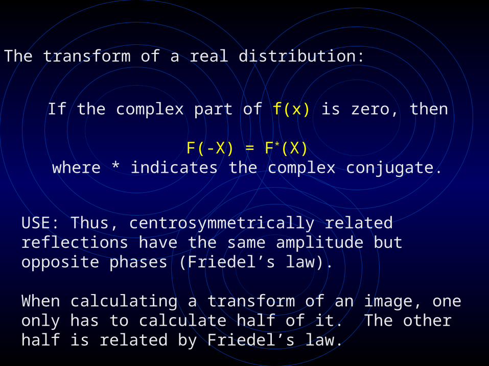
9. The transform of a real distribution:
If the complex part of f(x) is zero, then
F(-X) = F*(X)where * indicates the complex conjugate.
USE: Thus, centrosymmetrically related reflections have the same amplitude but opposite phases (Friedel’s law).
When calculating a transform of an image, one only has to calculate half of it. The other half is related by Friedel’s law.

10. Whatever applies to the FT also applies to the IFT.
USE: If the Fourier transform of a cosine wave is a pair of delta functions, then the inverse Fourier transform of a cosine wave is also a pair of delta functions.

Convolution of a molecule with a lattice generates a crystal.
Molecule = f(x)
lattice = l(x)
Set a molecule down at every lattice point.
f(x)*l(x)
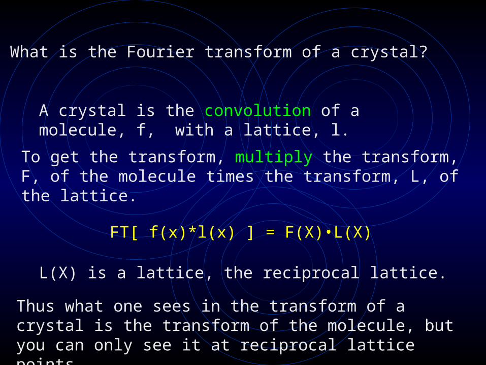
What is the Fourier transform of a crystal?
A crystal is the convolution of a molecule, f, with a lattice, l.
L(X) is a lattice, the reciprocal lattice.
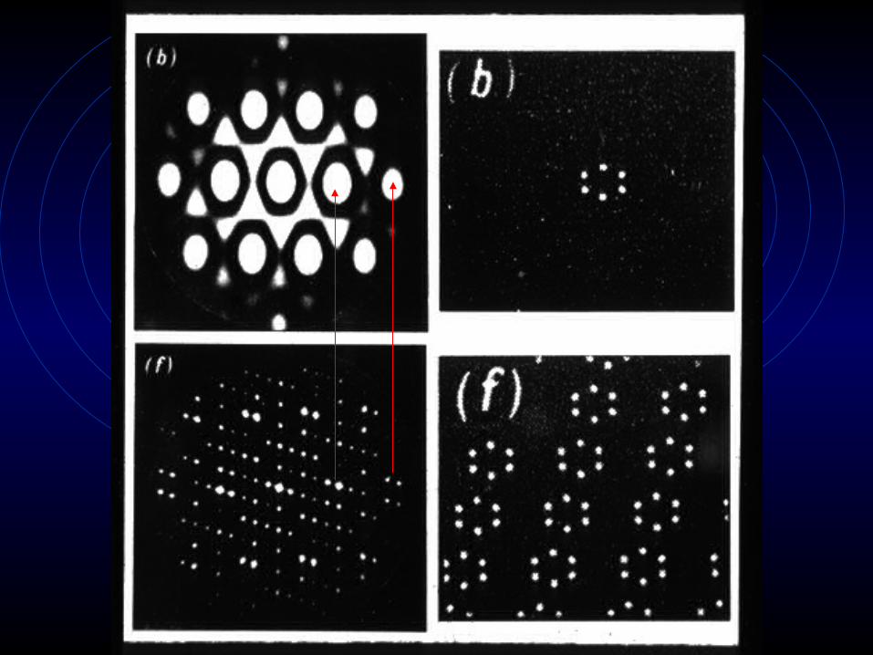
Thus what one sees in the transform of a crystal is the transform of the molecule, but you can only see it at reciprocal lattice points.
FT[ f(x)*l(x) ] = F(X)•L(X)
To get the transform, multiply the transform, F, of the molecule times the transform, L, of the lattice.

What is the Fourier transform of a sampled (digitized) image?
A sampled image is the product of a molecule, f, with a lattice, l.
L(X) is a lattice, the reciprocal lattice.
Thus what one sees is the transform of the molecule repeated at every reciprocal lattice point.
FT[ f(x)•l(x) ] = F(X)*L(X)
To get the transform, convolute the transform, F, of the molecule with the transform, L, of the sampling lattice.
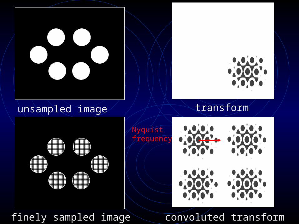
unsampled image transform
finely sampled image convoluted transform
Nyquistfrequency
Since the transform extends infinitely in all direction, the convolution causes overlap of one transform with its neighbors.
This is called aliasing.
The problem can be appreciated if we more coarsely sample the molecule in the previous example.
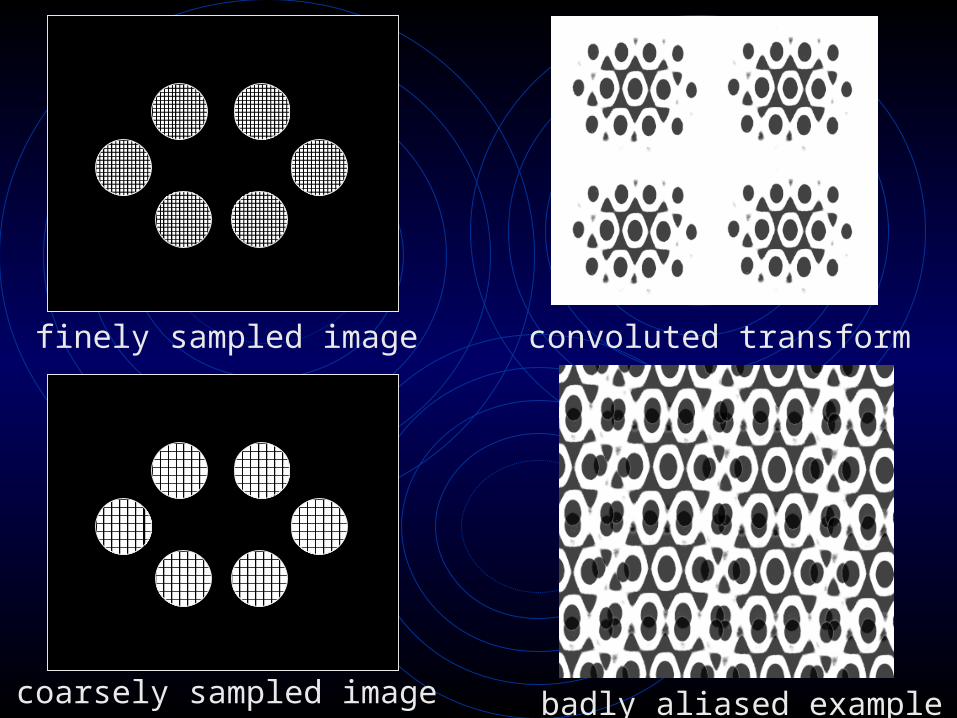
finely sampled image convoluted transform
coarsely sampled image badly aliased example
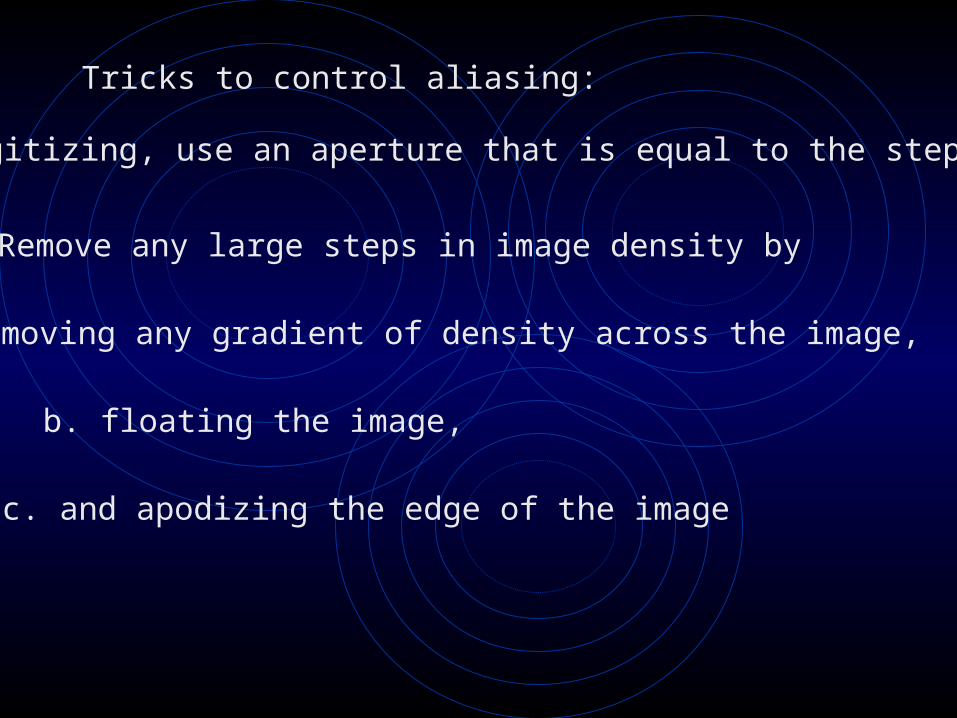
Tricks to control aliasing:
1. In digitizing, use an aperture that is equal to the step size.
2. Remove any large steps in image density by
a. removing any gradient of density across the image,
b. floating the image,
c. and apodizing the edge of the image
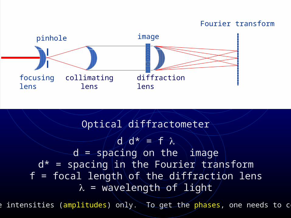
collimatinglens
diffractionlens
image
Fourier transform
pinhole
focusinglens
Optical diffractometer
d d* = f d = spacing on the image
d* = spacing in the Fourier transformf = focal length of the diffraction lens
= wavelength of light
One gets the intensities (amplitudes) only. To get the phases, one needs to compute the FT.

Fourier transforms have both real and imaginary parts.
The real part:
FR(X=1/a) = f(x)•cos(360x/a)
The imaginary part:
FI(X=1/a) = f(x)•sin(360x/a)

One can turn the real and imaginary parts into amplitudes and phases.
Amplitude:
|F(X=1/a)| = (FR *FR + FI *FI )1/2
Phase:
(X=1/a) = tan-1(FI /FR )
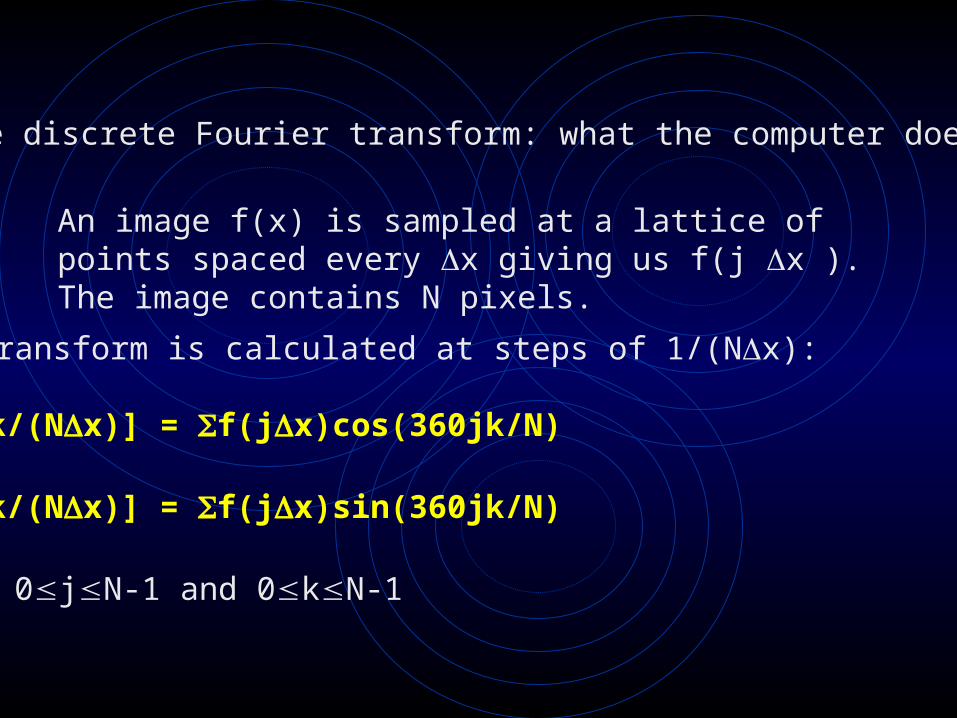
The discrete Fourier transform: what the computer does.
An image f(x) is sampled at a lattice of points spaced every x giving us f(j x ). The image contains N pixels.
The transform is calculated at steps of 1/(Nx):
FR[X=k/(Nx)] = f(jx)cos(360jk/N)
FI[X=k/(Nx)] = f(jx)sin(360jk/N)
where 0jN-1 and 0kN-1
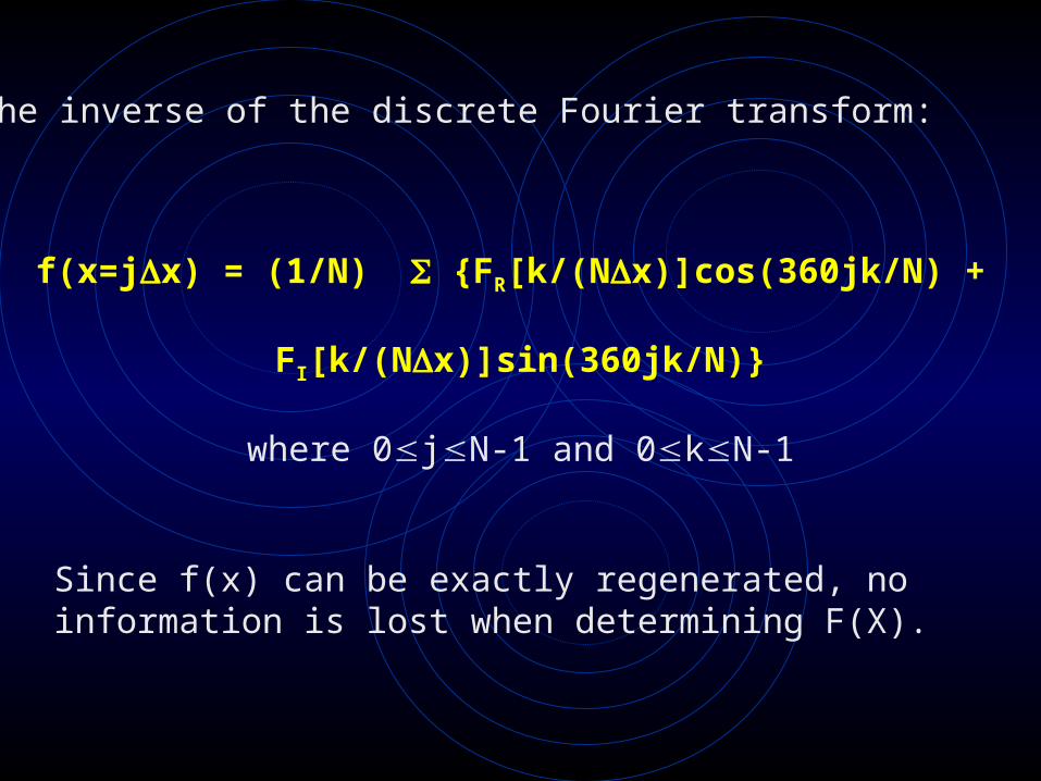
The inverse of the discrete Fourier transform:
f(x=jx) = (1/N) {FR[k/(Nx)]cos(360jk/N) +
FI[k/(Nx)]sin(360jk/N)}
where 0jN-1 and 0kN-1
Since f(x) can be exactly regenerated, no information is lost when determining F(X).
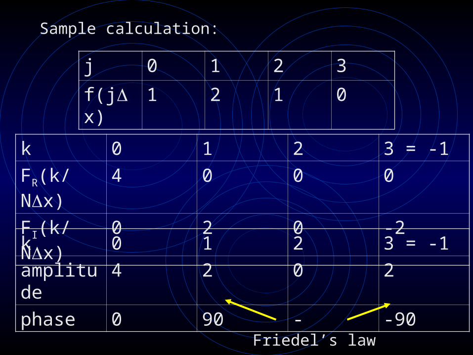
Sample calculation:
j 0 1 2 3
f(jx) 1 2 1 0
k 0 1 2 3 = -1
FR(k/Nx) 4 0 0 0
FI(k/Nx) 0 2 0 -2
k 0 1 2 3 = -1
amplitude 4 2 0 2
phase 0 90 - -90
Friedel’s law

What happens if we more finely sample the image?
Image f(x) is sampled at x/2 instead of x; it contains 2N instead of N pixels.
The transform is sampled at 1/(2Nx/2) = 1/(Nx); i.e. unchanged. However, since there are 2N instead of N steps, the resolution is twice as good.
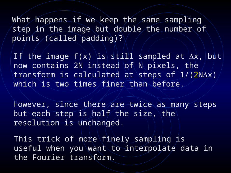
What happens if we keep the same sampling step in the image but double the number of points (called padding)?
If the image f(x) is still sampled at x, but now contains 2N instead of N pixels, the transform is calculated at steps of 1/(2Nx) which is two times finer than before.
However, since there are twice as many steps but each step is half the size, the resolution is unchanged.
This trick of more finely sampling is useful when you want to interpolate data in the Fourier transform.


![URBAN MORPHOLOGY some (very general) geometrical regularities [graphics from The Human Mosaic by Terry Jordan-Bychkov and Mona Domosh]](https://img.pdfslide.net/doc/110x75/56649dbb5503460f94aacaf0/urban-morphology-some-very-general-geometrical-regularities-graphics-from.jpg)

![On Some Regularities ofSubject and Topic Prominence Sang … · 2020. 6. 25. · On Some Regularities ofSubject and Topic Prominence Sang-HwanSeong ... ess-ta] John-nom/top[Mary-nomself-acelove-decl-comp)](https://img.pdfslide.net/doc/110x75/60b924ab9389ba3d5451b72b/on-some-regularities-ofsubject-and-topic-prominence-sang-2020-6-25-on-some.jpg)


![Protein-Protein Docking - cs.princeton.edu · 3 Binding Site Analysis Some residues have higher propensity to be in site [Jones00] Binding Site Analysis Residues in protein-protein](https://img.pdfslide.net/doc/110x75/5cee28b388c993f1758c2b9c/protein-protein-docking-cs-3-binding-site-analysis-some-residues-have-higher.jpg)