A Hybrid Geospatial Data Clustering Method for Hotspot ...journals.iau.ir/article_616_eab6c547b3540c00675ed259ece5446d.pdf · eliminate the deficiency, relatively modern data mining

Journal of Computer and Robotics 1 (2010) 53-67

53

A Hybrid Geospatial Data Clustering Method for Hotspot Analysis

Mohammad Reza Keyvanpoura *

, Mostafa Javidehb, Mohammad Reza Ebrahimi

c

a Department of Computer Engineering, Alzahra University, Tehran, Iran

bShamsipoor Technical College, Tehran, Iran c Islamic Azad University, Qazvin Branch, Qazvin, Iran

Received 10 February 2009; revised 28 October 2009; accepted 12 November 2009

Abstract

Traditional leveraging statistical methods for analyzing today’s large volumes of spatial data have high computational burdens. To eliminate the deficiency, relatively modern data mining techniques have been recently applied in different spatial analysis tasks with the purpose of autonomous knowledge extraction from high-volume spatial data. Fortunately, geospatial data is considered a proper subject for leveraging data mining techniques. The main purpose of this paper is presenting a hybrid geospatial data clustering mechanism in order to achieve a high performance hotspot analysis method. The method basically works on 2 or 3-dimensional geographic coordinates of different natural and unnatural phenomena. It uses the systematic cooperation of two popular clustering algorithms: the AGlomerative NEStive, as a hierarchical clustering method and κ-means, as a partitional clustering method. It is claimed that the hybrid method will inherit the low time complexity of the κ-means algorithm and also relative independency from user’s knowledge of the AGNES algorithm.

Thus, the proposed method is expected to be faster than AGNES algorithm and also more accurate than κ-means algorithm. Finally, the method was evaluated against two popular clustering measurement criteria. The first clustering evaluation criterion is adapted from Fisher’s separability criterion, and the second one is the popular minimum total distance measure. Results of evaluation reveal that the proposed hybrid method results in an acceptable performance. It has a desirable time complexity and also enjoys a higher cluster quality than its parents (AGNES and κ-means). Real-time processing of hotspots requires an efficient approach with low time complexity. So, the problem of time complexity has been taken into account in designing the proposed approach.

Keywords: Geospatial data; Geographical knowledge discovery; Hotspot analysis; Hierarchical clustering; Partitional clustering; Hybrid clustering

approach; Earthquake hotspots; Crime mapping.

1. Introduction

Recently, we are witnessing a growing tendency among

researchers to apply modern data mining techniques, on

geographical data, as one of the most essential steps of

KDD (Knowledge discovery from data) process. The

reason might be the fact that traditional statistical methods,

particularly spatial statistics are confirmatory and require the researcher to have a priori hypothesis, meaning that

they cannot discover unexpected or surprising information

[1].

KDD is the higher level process of obtaining facts

through data mining and distilling this information into

knowledge or ideas and beliefs about the mini-world

described by the data. This generally requires a human-

level intelligence to guide the process and interpret the

results based on pre-existing knowledge [2]. GKD

(Geographical Knowledge Discovery) is an extension of

the broader trend of KDD which is based on a belief that

there is novel and useful geographic knowledge hidden in

the unprecedented amount and scope of digital geo-

referenced data [2]. The current methods for exploratory

spatial analysis and spatial data mining span across three

main groups: computational, statistical, and visual

approaches [3]. This paper mainly addresses the first group. Computational approaches resort to computer algorithms to

search for large volumes of data for specific types of

patterns such as spatial clusters [4], spatial association rules

[5] and spatial outliers [6].

In general, computational methods are able to search for

structures in large datasets with great efficiency but lack

the ability to interpret and attach meaning to patterns [3].

Statistical methods are rigorous and verifiable but often

assume a priori model which has been roughly

predetermined by the analyzer [3].Geospatial Hotspot

analysis is one of the most vital tasks in the process of

*Corresponding author. E-mail: [email protected]

M.R. Keyvanpour et al. / A Hybrid Geospatial Data Clustering Method for Hotspot Analysis.

54

GKD which means finding the notable geographical

regions of natural/unnatural phenomena according to some interesting measures. The most general techniques

available for discovering geospatial hotspots are the mean

center, standard deviation distance, standard deviation

ellipses, and geospatial data clustering. All of these

techniques, except for clustering, are usually considered as

statistical techniques.

Clustering can be defined as dividing/discretizing a

dataset – commonly consisting of homogenous objects –

into subsets, each of which contains the most similar

objects, while every pair of subsets should have the highest

contrast. In fact, defining a proper distance measure will

force similar objects to be placed inside one cluster at the end of the clustering process. Therefore, the label for each

cluster will be unknown until the clustering process is

finished. Because of that, clustering problems are also

known as unsupervised learning methods.

Presenting an efficient method for clustering geospatial

data collected from diverse sources is a challenging task.

This paper mainly discusses the leveraging of a high-

performance approach for discovering geospatial hotspots

via employing the clustering of 2-D geospatial data. The

proposed method utilizes a systematic hybrid approach by

combining AGNES as a hierarchical and κ-means as a partitional clustering algorithms. The paper will examine

the subject by providing a brief accounts of two case

studies in a practical way. In the first case study, analyzing

crime incidents' location data for discovering geospatial

crime hotspots was conducted and the second case study is

concerned with seismological hotspot analysis. Eventually,

the method was tested and evaluated through utilizing it on

a georeferenced data set containing geographical

coordinates (longitude and latitude) of seismic activities in

Iran.

This paper is organized in seven main sections.

Following the introduction, section 2 provides a general background on the related works as well as recent

progresses. Section 3 discusses the most popular methods

for spatial data clustering and hotspot analysis as an

essential part of mapping natural and unnatural phenomena.

The fourth section mainly deals with preparing a

background to leverage three different clustering

techniques for hotspot analysis. The proposed hybrid

approach (HAK) will be introduced in section 5. In section

6, some of the most popular evaluation criteria (Fisher’s

separability criterion and minimum Total Distance) are

introduced, after which the proposed hybrid technique is evaluated on the basis of those criteria. Eventually, the last

section presents the conclusion and the authors’ scheduled

future works.

2. State of the Art

Utilizing spatial/geographical (see the difference in [2])

data mining is a rapidly-growing field of study in most

industries, enterprises and research areas. Hence,

presenting a comprehensive background on the subject

requires a complete book chapter. For the sake of briefness, we will focus on two geospatial hotspot analysis problem

domains: 1) crime incidents' location spatial analysis and

2) earthquake hotspot discovery. For clarity reasons, we

will divide this section into two main subjects and will keep

these two problems for the rest of the paper.

2.1. Crime Analysis

Recently, traditional crime analysis techniques have lost

their popularity in light of the new, less costly, and less

time-consuming analytical techniques. Additionally, using

computer-based analysis of crime data has had an

undeniably positive influence on the police force’s human

resource management. Generally, analyzing crime data includes both behavioral analysis (see [7-11]) and spatio-

temporal analysis. Due to the subject of the paper, we focus

on modern crime hotspot analysis which is considered as a

young field of study built upon new data mining

techniques.

Crime mapping is thoroughly elaborated on in [12]. In

[13], exploiting the spatial analysis for finding the proper

place for establishing the new police stations has been

discussed in detail. In [8], the writers have used

association-rule mining for extracting spatio-temporal

patterns out of large volumes of crime-related data. DBSCAN clustering technique has been utilized to design

and implement a spatial data engine and visualization

interface for a crime information system in [15]. In [16] a

model, named STEM, has been introduced to find frequent

rules among events, hotspots and time points. Another

interesting spatial clustering method which is called U-

Matrix has been discussed in [17].

A dynamic pattern analysis framework, the DPA

framework, has been presented in [18]. This framework

allows users to identify three types of dynamic patterns in

spatio-temporal data: 1) Similar spatial patterns at different

time points, 2) interactive relationship between two geographical locations as a result of specific reason, and 3)

frequent association rules related to particular types of

events, geographical locations and time points.

AIM (Action Information Management) software system

in England [19], benefits from spatial data in order to do

crime matching. This software depicts the results of results

in geographical maps. For example, results are shown as

offender crime corridors in a particular city map. These

corridors are identified by processing the locations’

coordinates of crime incidents which are related to a

specific offender. The United States’ CrimeStat software system processes

spatio-temporal data according to a statistic-based approach

and data mining techniques. Also, this system is capable of

estimating the approximate locations of future crimes.

Hotspot analysis is also covered in this software by means

of hierarchical nearest neighbor clustering algorithm, κ-

means algorithm and also a particular algorithm named

STAC (Spatial and Temporal Analysis of Crime) [20].


55

Fig. 1. Identifying the robbery hotspots using the STAC algorithm in Baltimore County by CrimeStat software [20].

Figure 1 depicts the clustering of street robberies in west

Baltimore County using the STAC clustering approach. As

the results indicate, there is a considerable concentration of

the robberies around one of the main outgoing highways of

the city which are colored in green.

The performance of hotspot analysis applications might

be dependent on doing some efficient optimizations on corresponding hotspot discovering algorithms. In [21],

writers prove that it is necessary to support an optimization

strategy –which is introduced as Join Index- in a hotspot

discovery application for increasing the performance of

identification of the hotspots; otherwise, this operation may

take 2 hours for a dataset size of 15000 crime reports.

2.2. Earthquake Spatial Analysis

Discovering the earthquake hotspots plays an important

role in Seismological researches. In fact, hotspot

identifications can help the researcher to model the seismic

activities of the earth in order to predict the approximate locations of the future earthquakes. The mentioned

activities facilitate making suitable decisions concerning

the scope of risk management problems. As an example, in

[22], a modeling approach for earthquake aftershocks has

been presented and tested based on the epidemic type

aftershock (ETAS) model introduced thoroughly in [23].

This model aims at modeling complex aftershocks’

sequences and global seismic activity [24], and it has been

used to give short-term probabilistic forecast of seismic

activity [24], and to describe the temporal and spatial

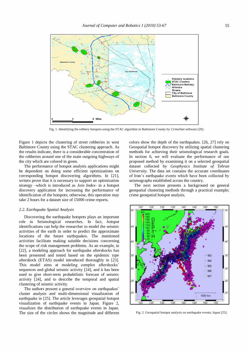
clustering of seismic activity. The authors present a general overview on earthquakes’

cluster analysis and multi-dimensional visualization of

earthquake in [25]. The article leverages geospatial hotspot

visualization of earthquake events in Japan. Figure 2,

visualizes the distribution of earthquake events in Japan.

The size of the circles shows the magnitude and different

colors show the depth of the earthquakes. [26, 27] rely on

Geospatial hotspot discovery by utilizing spatial clustering

methods for achieving their seismological research goals.

In section 6, we will evaluate the performance of our

proposed method by examining it on a selected geospatial

dataset collected by Geophysics Institute of Tehran

University. The data set contains the accurate coordinates of Iran’s earthquake events which have been collected by

seismographs established across the country.

The next section presents a background on general

geospatial clustering methods through a practical example;

crime geospatial hotspot analysis.

Fig. 2. Geospatial hotspot analysis on earthquake events; Japan [25].


56

(a)

(b)

Fig. 3: (a) Non-clustered vehicle crime points in London; (b) Density-based clustering for robbery [30].

3. A Practical Example: Overview of Popular Methods

for Crime Hotspot Analysis

The geographical coordinates of natural/unnatural

phenomena can be considered as the most important kinds of geographical data in geospatial data bases. Hotspot

exploration is considered a proper subject for applying

clustering techniques. The foundation of crime hotspot

analysis and its most popular methods are discussed in

detail in the following sub-sections.

Simply stated, the main purpose of hotspot analysis

process is to find places where the frequency of crime

occurrence is higher than other places. Finding these places

requires clustering analysis on crime spatial data. Doing

hotspot analysis on high-volume crime spatial data, without

using computerized clustering process, is almost impossible since using manual methods to find hotspots increases the

possibility of unintended human recognition mistakes.

Instead, employing clustering techniques with proper

visualization of results leads to an accurate hotspot analysis

process. It is considerable that crime hotspots have a

dynamic nature and they may change through time, so it

requires continuous monitoring over time. In other words,

the underlying pattern among the geospatial data might be

changed by adding new crime incidents.

As a practical example, robbery occurrence rate is more

concentrated in commercial centers and also busy avenues of the cities. These places can be identified accurately by

using hotspot analysis. Predicting location of the next

crime, estimating the offender living place, identifying

offenders’ crime corridors, optimizing police patrol routes

and offering the best place for the establishment of new

police stations are other important usages of crime hotspot

analysis. These applications are discussed in more details in

[28]. In what follows, the most common hotspot analysis

methods and their advantages /disadvantages are presented.

3.1. Point Maps

The Point mapping approach can be considered as one

of the most popular methods for analyzing crime hotspots

and visualizing the results. The popularity of this method lies in its simplicity as well as its similarity to the

traditional pins in map method [29]. As the name of the

method reads, crime incident’s geographical coordinates

are simply marked in a geographical map. The most

significant disadvantage of this method is its lack of

accuracy in identifying hotspots especially when there are

relatively huge amounts of data to be analyzed. Figure 3.a

depicts 9314 instances of vehicle crime occurred in London

marked by point mapping approach. The figure reveals that

not only identifying hot spots through this method is a

difficult task, but also the quality of analysis is tightly dependent on human recognition, because the method gives

no idea about data clustering!

3.2. Density-based Surface Mapping

This type of crime mapping utilizes density-based

clustering methods. The main purpose of this category of

clustering techniques can be summarized as gaining an

estimation of distribution of crime density across

geographical areas and also visualizing the results. The

ability of this method in finding clusters with arbitrary

shapes affords results that are similar to the real-world

distribution of objects. For visualizing the output of this method, a number of different colors should be chosen.

Each color represents a range of crime density in

corresponding area. Therefore, the method will divide the

surface to some colored zones with arbitrary shapes.

Choosing the number of these colors (zones) has a

significant influence on clustering quality, so it should be

chosen intelligently. Figure 3.b shows density-based


57

clustering method for robbery crime incidents in London.

Realizing crime hotspots is also possible by using other clustering methods like hierarchical or partitional clustering

methods.

3.3. Geographic Boundary Thematic Mapping

This kind of hotspot analysis is distinct from other

methods as it enters the provincial boundaries or other

districts’ geographical boundaries in the analysis process.

In this method, every predetermined geographical region is

colored according to the crime occurrence rate

concentration. Coloring strategy is one of the most

important steps for creating maps using this method (see

[30]). As already mentioned, the number of colors chosen

to discretize the surface of the map plays an important role in crime mapping. There are several measurement criteria

for discretizing the surface of the target area. Using the

standard deviation or the ratio of the occurred crimes to

the population of a specific area may be appropriate as

crime occurrence concentration criteria. The quality of hot

spot analysis process depends on choosing the

concentration criteria as well as the number of colors for

discretizing the surface. Designating the number of colors

less than a proper value may result in decreasing the

analysis accuracy; on the other hand, choosing a number

greater than the proper value will lead to complexity of interpreting the analysis results. Using 5 or 6 different

colors/states is optimal for covering the most hotspot

problems [30]. Using the geographical boundary thematic

mapping method is a useful approach for accomplishing

crime reduction strategies in a specific geographical area. It

also aids police services to realize crime management

programs. It is worth knowing that this method assigns a

constant density value to a relatively vast geographical

zone. This behavior results in lack of accuracy and it might

be considered as a drawback.

3.4. Grid-based Mapping

This crime mapping approach originates from grid-based clustering methods. Grid-based clustering is different

from other clustering methods in the way it operates on the

target data set. That is, rather than discretizing the data set

objects, it discretizes the state space in which objects are

resident (see [31]). Each object is assigned to a state space

division according to the parameters of the algorithm.

Being independent from the order of the data objects is

considered as an important advantage of grid-based

clustering method. Simply stated, the crime mapping

process using grid-based clustering method has two main

steps. The first step is dividing the target geographical surface into some square-shaped cells with equal areas. The

next step is assigning each crime incident to an appropriate

cell according to the frequency of incidents occurred in the

corresponding cell surface. This kind of crime mapping

usually does well in performance but it suffers from some

drawbacks. The followings may be considered as some of

the most important drawbacks of grid thematic crime

mapping:

Naturally, the shapes of hotspots are irregular due to

the distribution of crime incidents in the real-world, but

because the method uses square-shaped grids it is not able

to generate arbitrary shapes.

The analysis result extremely depends on the size of

cells. So, different sizes will result in different hotspot

interpretations. Dividing the target surface into a low

number of grids will result in losing details. Also, dividing

the surface into too many cells makes the output

uninterpretable.

Figure 4 demonstrates the output of this kind of crime

mapping method used for burglary crimes in London by Metropolitan Police. If the area of the cells is chosen

wisely, it will be expected that the output will be more

accurate than geographic boundary mapping output. As it

can be seen in Figure 4, there are 4 levels of crime

concentration (1 to 5, 5 to 10, 10 to 15 and more than 15).

Fig.4. Crime mapping by using grid based method-London [30].

4. Utilizing Clustering Techniques for Hotspot

Discovery

In this section, some advantages and disadvantages of

the AGNES method, as a hierarchical clustering method

and κ-means, as a partitional clustering method are

discussed. As pointed out earlier, there are several methods

for spatial data clustering. Choosing the proper method can

be affected by the problem domain. Also, designating a

proper distance measure is considered as a main

prerequisite of all kinds of clustering processes (see [32]). Again, as it was mentioned earlier, Geospatial data sets

usually contain data objects in the form of 2-dimensional


58

points’ coordinates (X, Y) which can be mapped in a

geographical map. Normally, Euclidian Distance measure is used for the purpose of crime spatial data clustering.

Spatial data clustering is widely used in hotspot analysis of

georeferenced data.

4.1. Hotspot Analysis Using the AGNES Clustering

Algorithm

Hierarchical clustering methods can be divided into two

categories [32]: 1) Methods which are based on

agglomerative algorithms and 2) Methods based on divisive

algorithms. In the earliest step of agglomerative algorithms,

each data object is considered as a cluster. Then, the

distance/dissimilarity between each pair of clusters is

computed. The two clusters with the most similarity will be merged into one cluster. This sequence of operations will

be continued until reaching a predefined number of clusters

or a predefined inter-cluster distance. There are multiple

strategies for calculating the distance between two clusters.

For example, in centroid strategy, the distance between two

different clusters can be defined as the distance between

each cluster’s centroid. Centroid of each cluster is the

average of objects’ distances within that cluster. Another

strategy for calculating inter-cluster distance is the average

strategy which uses the Equation (1) for measuring the

distance between two clusters.

𝑑(𝐶𝑖 ,𝐶𝑗 ) =1

𝑛 𝑖𝑛 𝑗 |p − p′ |p ′ ∈C j

p∈C i

(1)

In this equation, the distance between cluster 𝐶𝑖, having

ni objects within it, and cluster 𝐶𝑗 , having nj objects, is

defined as the average of the summation of the distances

between each object within 𝐶𝑖 and all objects within 𝐶𝑗 .

Each level of the naive AGNES clustering process [32]

can be recorded in a hierarchical structure (dendogram)

located in memory. So, it will be possible to access the

process result in each level of executing the algorithm and

then choose the better answer according to some criteria. In

other words, the progression of the clustering process will

be visible through using this method. Also, it will be

possible to use the result of each level in a separate

algorithm. Although this is considered as an important

benefit of this method in comparison to other clustering algorithms, it should be noted that saving the clustering

hierarchy in memory will result in additional memory

consumption. Nevertheless, the other advantage of this

algorithm is being relatively independent from human

knowledge for initializing the algorithm. For Example, it

does not require the user to specify the primary seeds for

the algorithm to be initialized.

This method has the time-complexity of O(n3). It uses an

n×n distance matrix (n is the number of data objects

supposed to be clustered); therefore, the algorithm has the

order of O(n2) spatial complexity [33]. So, the AGNES method is suffering from the relatively high time-space

complexity. This behavior causes the method to be

practically useless in dealing with high-volume data.

Unfortunately, due to the large amounts of data which are often used for crime hotspot analysis, exploiting the

AGNES method does not seem cost-effective.

4.2. Hotspot Analysis Using the κ-means Clustering

Algorithm

The most significant feature of partitional clustering

algorithms, especially κ-means, is their relatively low time

complexity. One of the main reasons for the popularity of

this type of clustering algorithms is its adaptability when it

encounters large volumes of data [32]. Nevertheless,

convergence of the results of this method to local optimums

rather than global optimums is considered as a drawback, in

comparison to hierarchical clustering algorithms (see [33]). Anyway, κ-means and its newer variations are currently

considered as popular methods in hotspot analysis as well

as other fields of study.

The naive κ-means algorithm [32], in the first step,

selects some data objects randomly as primary seeds which

are named as centroid. Each centroid represents a cluster.

Then the distances between all of the data objects with each

of the centroids will be calculated. Each data object will be

assigned to the cluster which is containing the nearest

centroid. As the next step, the average of the data objects

within each cluster will be computed as the new centroid of the corresponding cluster and the mentioned steps repeat

until the result of clustering remains with no change or a

predefined convergence criterion satisfied. MSE (Min

Squared Error) is a common convergence criterion which is

calculated by Equation (2) [33].

𝐸 = 𝑝 − 𝑚𝑖 2

𝑝∈𝐶𝑖

𝑘

𝑖=1 (2)

In Equation (2), |𝑝 − 𝑚𝑖|, represents the distance of

object p from the centroid of its containing cluster 𝐶𝑖 . K is the number of clusters and finally, E is the summation of

mean squared error of clusters. Using MSE leads to

maximizing inter-cluster distance and minimizing intra-

cluster distance. The followings are some of the most

notable disadvantages of the classic κ-means algorithm:

The algorithm requires preliminary knowledge to be

initialized; specifying the number of clusters or even

cluster’s centroids are needed for the algorithm to get

started. Otherwise, the algorithm will choose the centriods

randomly.

The result of clustering is highly dependent on the

selected primary centroids; selecting non proper seeds will

result in unexpected behaviors.

Computing the data objects mean is extremely

sensitive to outliers.

There is not any standard approach for selecting the

primary seeds wisely.

There is no guarantee that algorithm converges to

global optimum; sometimes it converges to local optimums.


59

In spite of the fact that the classic κ-means algorithm has

many considerable drawbacks, it is a common algorithm because of its low time-space complexity (Ο(n)).

5. The Proposed Hybrid Method (HAK)

This section presents the proposed method. The rough

idea for combining the parent algorithms can be described

as follows: First, m iterations of the AGNES algorithm are

executed; so, some clusters will be found and the execution

of the AGNES will be interrupted. As the next step, the

result of the AGNES algorithm will be passed to κ-means

as its initializing inputs (seeds). Then κ-means algorithm

will do the rest of the clustering job.

How many AGNES iterations are enough to be run? The

answer will solve a significant sub-problem in the issue of combining two mentioned algorithms. It should be noted

that executing too many iterations of the AGNES

Algorithm will enforce the hybrid algorithm to behave like

a pure hierarchical algorithm and, as a result, it has its own

mentioned disadvantages. On the other hand, if a rather

slight number of the AGNES iterations is executed,

clustering results will not be of desirable quality because of

non-proper primary centroids.

5.1. The Parameters of the Proposed Method

According to the previous discussions, it can be realized

that specifying the m parameter is the key solution of this hybrid approach. m is the number of the iterations of the

AGNES algorithm. It is also possible to tune m parameter

indirectly by manipulating the distance threshold of the

AGNES algorithm (T). The AGNES distance threshold is

the maximum inter-cluster distance which is considered as

a stop value for the most hierarchical algorithms [32]. At

any rate, using this hybrid method, there is no need to

specify the initializing parameter(s) of the classic κ-means

algorithm directly. In fact, the proposed method can be

manipulated by means of three parameters which are

introduced subsequently. Although initializing these

parameters is optional, if they are set wisely, the performance will be improved significantly.

Parameter m: Specifies the number of iterations of the

AGNES algorithm.

Parameter T: Specifies the AGNES algorithm’s threshold

as defined above.

Parameter λ: Specifies the minimum number of data

objects that a cluster should contain to be involved in the κ-

means algorithm. In other words, valid clusters must have

at least λ objects within them.

As a matter of fact, the first two parameters will tune the

AGNES algorithms and the last one will adjust the κ-means algorithm. Usually, initializing the input parameter of the

naive AGNES clustering algorithm requires setting the

number of output clusters. The value of this parameter will

be equivalent to the difference between the number of

entities in dataset and the mentioned parameter m. The

reason is that the AGNES algorithm will certainly merge

two clusters of the dataset in each iteration of execution [33]. Some notable guidelines for specifying the parameter

m are stated in the following sections.

5.1.1. Identifying the Upper Bound of Parameter m

As already discussed, combining the above-mentioned

clustering methods, requires finding an upper bound for

parameter m to limit its domain. If the value for m is chosen

to be more than a specific threshold, certainly, the proposed

method will have more time-space complexity than the

classic AGNES algorithm. Identifying an upper bound

value for m is considered as an essential requirement for

obtaining a rational performance justification for the hybrid

approach. So, it is recommended that the value of m do not exceeds a calculable threshold. As a rough estimation, let n

be the number of data objects in the target clustering data

set. In the case of using the naive AGNES clustering

method, with centroid inter-cluster distance strategy,

running the first iteration of merging the nearest data

objects, requires n(n-1)/2 comparisons. Thus, in the second

iteration (n-1)(n-2)/2 comparisons are needed to select the

two nearest data objects. As the worst case scenario for the

proposed method, suppose a situation in which an entire κ-

means algorithm process is executed immediately after

finishing each iteration of the AGNES process. Consequently, [(n)(n-1) /2]+ n comparisons is required in

the first iteration of the proposed method. So, the following

equations can be used as a rough estimation:

Required number of comparisons in the naive AGNES

algorithm:

𝑛 𝑛 − 1 + 𝑛 − 1 𝑛 − 2 + 𝑛 − 2 𝑛 − 3 + ⋯+ 2 × 1

+1 × 0 = 𝑘( 𝑘 − 1 𝑛

𝑘=1; (3)

Required number of comparisons in hybrid approach

(worst case scenario):

1/2 𝑛 𝑛 − 1 + 𝑛 + 𝑛 − 1 𝑛 − 2 + 𝑛 + ⋯+ 2 × 1+ 𝑛 + 1 × 0 + 𝑛 =

𝑛2 + 1/2[𝑛 𝑛 − 1 + 𝑛 − 1 𝑛 − 2 + ⋯+ 𝑛 − 𝑝 𝑛 − 𝑝 − 1 + ⋯ + 2 × 1

= 𝑛2 + 1/2 𝑘(𝑘 − 1)

𝑛

𝑘=1

(4)

Equations (3) and (4) are in the form of summation of the

products. In Equation (3), each product term represents the

number of comparisons required in corresponding iteration

of the AGNES algorithm. Similarly, in Equation (4), each

product term represents the number of comparisons

required in the corresponding iteration of proposed hybrid

approach. In order to have the computational overhead of the hybrid method be less than the classic AGNES

algorithm, a specific number of terms in Equation (4)

should be computed rather than computing all of the terms.

This specific number of terms will be equal to n-p+1.


60

Let the maximum number of AGNES’ iterations be

𝑚𝑚𝑎𝑥 . As it is obvious in the Equation (4), the maximum number of included terms, which is actually equal to the

maximum number of iterations (𝑚𝑚𝑎𝑥 ), will be reached,

when the value of P is minimized. Let this minimum value

for P be 𝑃𝑚𝑖𝑛 . Then, the value for 𝑚𝑚𝑎𝑥 will be obtained

by Equation (5).

𝑚𝑚𝑎𝑥 = 𝑛 − 𝑝𝑚𝑖𝑛 + 1 (5)

Including 𝑛 − 𝑝𝑚𝑖𝑛 + 1 terms of the Equation (4), the

overhead which is generated by κ-means will be (n-p+1)n. Consequently, the upper bound of parameter m is

calculated from inequality (6).

(𝑛 − 𝑝 + 1)𝑛 + 𝑘(𝑘−1)

2 ≤

𝑘(𝑘−1)

2 ;𝑛

𝑘=1𝑛𝑘=𝑝 (6)

By expanding the inequality (6), we will obtain

inequality (7):

(𝑛 − 𝑝 + 1)𝑛 ≤ 𝑘(𝑘−1)

2 =>

𝑝−1𝑘=1

𝑛 − 𝑝 + 1 𝑛 ≤1

2 ( 𝑘2 − 𝑘

𝑝−1𝑘=1

𝑝−1𝑘=1 ) =>

𝑛 − 𝑝 + 1 𝑛 ≤ 1/2 𝑝−1 𝑝−2 2𝑝−3

6−

𝑝−1 𝑝

2 =>

6𝑛 𝑛 − 𝑝 + 1 ≤ 𝑝 − 1 (𝑝2 − 5𝑝 + 3) (7)

Now, we can determine the minimum value of p which

satisfies the above inequality (𝑝min ). By substituting n with

a proper integer, 𝑝min is obtained and

subsequently, 𝑚𝑚𝑎𝑥 will be obtained by Equation (5). It is worth mentioning that because of the integer nature of m,

there is no need to solve the mentioned third-degree

inequality. This implies that it will be solved by means of a

simple try-and-error approach. As an example, consider a

situation in which there are 648 objects in the target data

set (n=648). By substituting n in the inequality (7) the

following will be obtained:

6×648× (648-p+1) ≤ 𝑝 − 1 𝑝2 − 5𝑝 + 3 ;

The minimum value for p, pmin, which satisfies the

inequality (7) is 129. Subsequently the value of 𝑚𝑚𝑎𝑥 can

be calculated by the Equation (5) as follows: 𝑚𝑚𝑎𝑥 = n-

p+1= 648-129+1=520. Actually, this means that in order to have a rational computational complexity, the number of

the AGNES iterations in the proposed method must be less

than or equal to 𝑚𝑚𝑎𝑥 = 520.

In other words, if the number of the AGNES algorithm’s

iterations is chosen to be lower than 520 (i.e. equivalent to

129 clusters), the computational complexity of the

proposed method will be also expected to be lower than the

AGNES algorithm’s complexity. Although the proposed

algorithm will not force the user to select values which are

lower than mmax, it is notable that disobeying this rule will

cause the algorithm to behave like its hierarchical parent

AGNES. For example, if m=647 is selected, then the algorithm will be transformed into the pure AGNES, so, it

will lose the benefits we pointed out in section 5.1.

5.1.2. Identifying the Lower Bound of Parameter m

It was previously mentioned that the hybrid algorithm is

able to interact with the user. This means that a quality

evaluation sub-algorithm will be run to determine the

clustering result’s quality according to some criteria which

will be presented in section 6. If the user is not satisfied

with the clustering result, she/he will increase or decrease

the value of parameter m. It is likely that manipulating the

value of parameter m leads to a higher quality clustering.

Therefore, it is recommended that in the situations when the user has no knowledge about distribution of data, the

algorithm be initialized by the starting value of m=2. The

value will be increased gradually according to a method

introduced in the following sub-section. The lower bound

of parameter m varies for different clustering problems,

because it directly depends on the distribution of the data

objects. Thus, calculating the lower bound for each

different problem seems to be a complicated task.

Nevertheless, finding an accurate lower bound for

parameter m is useful to decrease the time complexity of

hybrid algorithm. This problem awaits further research by other researchers.

6. Evaluating the Algorithm

This section is mainly devoted to the comparative

performance evaluation of the proposed hybrid method,

classic AGNES and κ-means algorithms. Actually,

comparing two clustering algorithms is a laborious and

complicated task and there are various criteria to

accomplish this goal. Some of these criteria have single-

purpose usages and some others are widely applicable in

different domains. Unfortunately, there is not any all-

purpose clustering algorithm which satisfies all of the

existing criteria. Thus, the algorithms which perform well against a specific criterion often do not perform well from

the point of view of another criterion. In the following

sections, a combinational criterion, adapted from Fisher’s

separability criterion, is introduced. Fisher criterion is

considered as a widely applicable criterion [34]. Towards

the end of this section, the parent algorithms (AGNES and

κ-means) and the proposed hybrid method will be

evaluated.

6.1. Preparing the Evaluation Prerequisites

There are two main Prerequisites for evaluating the

algorithms: 1) understanding the data set origins and characteristics, and 2) a proper clustering evaluation

criterion. These two prerequisites are discussed in the

following two sub-sections.


61

Data Understanding: In order to examine the

performance of the previously mentioned mechanism, a dataset containing earthquake phenomena which occurred

in Iran in 2008 was selected from the collection of data sets

of Geophysics Institute of Tehran University [35]. The data

set includes a real collection of 2-dimentional earthquake

incidents, which contains 648 data objects. The data set

contains the accurate coordinates of Iran’s earthquake

events collected by seismographs established across the

country. So, the dataset is used widely in seismology

studies and the related experiments. Because the main

purpose of this paper is analyzing the 2-dimentional spatial

data, only the latitude and longitude of the data objects

were included in hotspot analysis. It should be noticed that none of the outliers was omitted in the data preparation

phase to see the algorithm’s behavior in dealing with

outliers.

Introducing the Criteria for Evaluation and

Comparison: Based on the simple definition of clustering,

it can be stated that measuring the amount of maximization

of inter-cluster distance and also the amount of

minimization of intra-cluster distance for an specific

algorithm seems an efficient clustering quality criterion

[36]. In fact, a clustering algorithm will support a desired

quality if it is able to satisfy the following two conditions simultaneously:

The distances between clusters which are determined

by the algorithm should be maximized.

The data objects in a specific cluster should be as

compact as possible.

Two popular clustering quality criteria are referenced to

in the current literature: Fisher’s separability criterion and

Minimum Total Distance. Simplified Fisher’s criterion

requires the calculation of Intra-cluster and Inter-cluster

variance as two popular clustering quality measures. These

measures will be calculated as follows:

1) Intra-cluster variance: Basically, variance measures the distribution of the data objects within a data set around

the mean value of that data set and it can be calculated by

Equation (8).

𝜎2 =1

𝑁 (𝑥𝑖 − 𝜇)2𝑁

𝑖=1 (8)

In the above equation, N represents the number of

objects in a data set and 𝜇 is the mean of the objects. This

criterion is usually used for measuring the distribution of

data objects within a cluster. Thus, the average of the

variance of the data objects within each cluster is

considered as the algorithm’s intra-cluster variance.

Henceforward, the intra-cluster variance measure will be

referenced as Var. So, if the result of running clustering

method C, includes n clusters, the value of the intra-cluster

variance will be calculated from Equation (9).

𝑉𝑎𝑟𝑐 =1

𝑛 𝜎2

𝑖𝑛𝑖=1 (9)

2) Inter-cluster variance: For computing the inter-

cluster variance of a specific clustering method’s result, the following algorithm was used;

a) The distance between cluster 𝑐𝑖 and 𝑐j is defined as

the average distance among all of the data objects within

cluster 𝑐𝑖 and the centroid of cluster 𝑐j . It can be calculated

by Equation (10).

𝑑 𝑐𝑖 , 𝑐𝑗 =1

𝑁 (𝑥𝑖 − 𝜇𝑗 )2𝑁

𝑖=1 (10)

In this equation, N represents the number of objects within

ith cluster. 𝜇𝑗 is the centroid of Jth cluster which is obviously

obtained by: 𝜇𝑗 =1

𝑀 𝑋𝑘

𝑀𝑘=1 ; M is the number of data

objects in jth cluster. b) Step a is repeated for all of the clusters which are

determined in the clustering results. The distances among

each cluster and all of the other clusters are computed. It

will result in generation of a scatter matrix. Inter-cluster

variance for cluster 𝑐i , which was named as Dic, is equal to the average of entries on each row of the matrix and it is

calculated by Equation (11).

𝐷𝑖𝑐 (𝑐𝑖) =1

𝑛−1 𝑑(𝑐𝑖 , 𝑐𝑗 )

𝑛

𝑗=1,𝑗≠𝑖 (11)

In Equation (11), n is the number of objects within 𝑐i

and {i,j∈ ℤ| 𝑖, 𝑗 ≤ 𝑛}. The equation represents how the

value of inter-cluster variance for cluster 𝑐𝑖 is calculated

using the previously-mentioned scatter matrix. Now, the

algorithm’s total inter-cluster variance can be calculated by

computing the average of all of the clusters’ Dic.

3) The ratio of inter-cluster variance to intra-cluster

variance: By combining the two mentioned criteria, a more

generic criterion is created which is the simplified form of

the Fisher’s criterion. Suppose that the result of the clustering method C, contains k clusters (C1,C2,…,Ck),

Then, the mentioned generic criterion can be calculated by

Equation (12).

𝑓 𝐶 =1

𝑘

𝐷𝑖𝑐 𝑐𝑖

𝑉𝑎𝑟 𝑖 𝑘

𝑖=1 (12)

In Equation (12), 𝑉𝑎𝑟𝑖 is the intra-cluster variance of ith

cluster and 𝐷𝑖𝑐 (𝑐𝑖) is the inter-cluster variance of cluster i,

which are obtained from the Equation (9) and (11).

According to this criterion, decreasing the intra-cluster

variance will result in decreasing the value of Vari and

consequently, increasing the value of f(c).

4) Minimum Total Distance: In this criterion, we

minimize the total of the sum of distances of objects to

their cluster centroids and the sum of the distances of the

cluster centroids from the global centroid [36]. Let a clustering assignment discrete the data set into m clusters

and Cj be one of the clusters. The value for Minimum Total

Distance is computed as follows:


62

𝑇𝐷 = 𝐷 𝑅𝑖 , 𝐶𝑗𝑐 𝑅𝑖∈𝐶𝑗

𝑚𝑗=1 + 𝐷 𝐶𝑗𝑐 , 𝐺𝑐

𝑚𝑗 =1 (13)

Where TD is the Minimum Total Distance for a specific

clustering assignment, Ri is an object in cluster Cj, 𝐶𝑗𝑐 is the

centroid of Jth cluster, and GC is the global centroid of the

data set. Finally 𝐷 𝑅𝑖 , 𝐶𝑗𝑐 is the distance between 𝑅𝑖 and

𝐶𝑗𝑐 . It is noteable that unlike the Fisher’s criterion, the

better clustering answers expect to have a lower number of

TD.

6.2. Evaluating the Parent Algorithms

The performance issues of the classic AGNES and κ-

means algorithms are discussed in this section. The

previously introduced criteria have been applied to

accomplish this goal. As already mentioned about test data

set, this set contains 648 earthquake incident’s coordinates.

Each algorithm was evaluated by f(c) and TD(c) measures. The former represents Fisher’s criterion value and the later

is the Minimum Total Distance value for the corresponding

algorithm.

6.2.1. Evaluating the Naive AGNES Algorithm

Table 1 demonstrates the value of Fisher’s criterion

(f(c)) for the various cluster’s quantities in the AGNES

algorithm. The average-link strategy was used as an inter-

cluster distance measuring strategy. As the table shows, the

maximum value for f(c) and the minimum value for TD(c)

occurred in the relatively low numbers of clusters and

moving toward the higher cluster’s quantities results in

reduction of the value for f(c) and increase of the value for

TD(c). In the other words, the more number of clusters we

choose, the worse clustering answer will be gained. It is

noteworthy that the outliers are merged in the latest iterations of the AGNES algorithm. Consequently, the

existence of the outliers among the objects of target data set

may cause deceptive results due to the increasing of f(c)

value.

Table 1

The evaluation of the AGNES algorithm by means of the f(c) and TD(c) criteria

Cluster quality Criterion

10 9 8 7 6 5 4 3 2

317.85 341.16 382.41 455.59 543.56 627.39 770.15 990.25 1274.02 f(c)

634.39 615.93 558.87 525.87 497.03 407.58 356.396 258.80 168.32 TD(c)

19 18 17 16 15 14 13 12 11

340.71 367.36 386.27 406.63 430.92 471.95 506.93 264.20 281.75 f(c)

1011.45 941.13 914.84 905.73 897.90 818.29 809.60 732.95 656.19 TD(c)

80 70 60 50 45 40 35 30 25

174.37 194.18 228.92 265.92 300.86 344.93 198.61 230.88 267.8 f(c)

1468.84 1420.36 1343.88 1290.07 1256.94 1221.47 1195.93 1093.33 1059.29 TD(c)

240 220 200 180 160 140 129 120 100

108.10 110.49 117.99 118.97 114.56 115.34 119.20 122.08 144.37 f(c)

2336.04 2243.31 2134.66 2021.85 1907.17 1812.19 1757.72 1694.98 1596.77 TD(c)

480 450 420 390 360 330 300 280 260

109.74 109.73 118.18 118.47 108.95 102.00 94.23 96.76 100.72 f(c)

3684.09 3548.40 3243.98 3099.44 2962.99 2796.93 2647.92 2538.24 2443.92 TD(c)

628 624 620 610 600 580 560 540 510

39.84 46.81 53.33 63.49 67.49 81.49 89.00 98.49 108.14 f(c)

4488.08 4468.82 4436.79 4380.09 4328.15 4164.75 4059.33 3964.46 3830.88 TD(c)

648 646 644 642 640 638 634 632 630

0 2.68 7.99 13.93 19.19 25.13 27.65 31.50 35.14 f(c)

4587.76 4582.73 4573.19 4559.94 4551.21 4538.83 4518.87 4509.54 4502.92 TD(c)


63

According to the Table 1, it can be realized that there are

several clustering results which own a relatively high quality and some of them may be preferred based on the

domain expert idea. If there are 648 data objects in the data

set, then the number of iterations of the naive AGNES

algorithm must be lower than 520 (equivalent to 129

clusters) to have a rational computational complexity (see

section 5). The related cell for this value is underlined in

the Table 2.

6.3. Comparative Evaluation

In this section, time and space complexity of the

proposed hybrid approach are compared to its previously

mentioned parents. Finally, the results of evaluation are represented as comparative diagrams. According to the

rough estimations mentioned in section 5, if assuming the

worst case in which the hybrid algorithm is initialized by

m=2 and also it is allowed to execute mmax iterations (mmax

is obtained by inequality (6) and Equation (7)), the

algorithm will have the computational complexity equal to the AGNES complexity. In the other situations where the

value of m is less than mmax, it is expected that the hybrid

method’s time complexity is also less than the AGNES

complexity. The HAK algorithm executed by λ=2 (λ is

defined in section 5-2 as a non-essential input parameter of

HAK).

6.3.1. Comparing HAK with AGNES

Figure 5 illustrates the evaluation results for the AGNES,

and the hybrid method (HAK). The horizontal axis of the

graph represents the number of AGNES iterations as an

independent parameter. The vertical axis represents the

values of f(c) criterion for each AGNES’ iterations. The areas that own a better clustering quality have been shown

in boxes. Interestingly, in some cases, the hybrid approach

has led to better results than the AGNES algorithm,

because it was expected to improve just clustering quality

of κ-means!

Table 2

The changes of the f(c) and TD(c) criteria in the κ-means algorithm

Cluster quality Criterion

10 9 8 7 6 5 4 3 2

278.38 308.81 347.08 397.17 440.02 504.93 289.08 225.03 3.43 Avg[f(c)]

317.87 310.58 297.90 295.73 277.23 261.96 179.02 117.51 37.92 Avg[TD(c])

19 18 17 16 15 14 13 12 11

157.14 164.07 172.39 182.10 192.18 205.93 218.80 235.61 255.49 Avg[f(c)]

395.90 391.29 378.53 368.50 356.95 345.64 351.63 342.84 318.78 Avg[TD(c])

80 70 60 50 45 40 35 30 20

94.93 84.66 83.46 88.20 96.54 90.90 102.46 111.26 149.87 Avg[f(c)]

830.70 770.32 705.72 623.59 612.197 588.58 519.93 508.27 409.98 Avg[TD(c])

240 220 200 180 160 140 120 100 90

117.75 119.55 116.00 107.30 106.11 91.87 93.00 89.86 83.70 Avg[f(c)]

1810.84 1714.89 1666.93 1455.36 1343.00 1166.90 1048.44 934.92 865.26 Avg[TD(c])

480 450 420 390 360 330 300 280 260

90.35 99.34 108.78 110.89 123.46 116.75 126.44 118.41 118.47 Avg[f(c)]

3472.61 3249.74 3035.12 2869.22 2610.29 2431.95 2254.95 2113.59 1990.36 Avg[TD(c])

628 624 620 610 600 580 540 520 510

12.439 14.85 16.52 24.37 29.55 43.29 59.16 73.78 75.34 Avg[f(c)]

4447.44 4430.45 4380.86 4315.36 4245.40 4105.21 3815.94 3762.78 3703.86 Avg[TD(c])

646 645 644 642 640 638 636 634 632

0.28 1.08 1.13 3.21 4.65 4.98 5.93 8.37 10.02 Avg[f(c)]

4581.25 4576.01 4568.28 4543.51 4535.56 4528.32 4517.10 4501.79 4486.69 Avg[TD(c])


64

Fig. 5. Comparing the clustering quality of AGNES and hybrid approach; from Fisher’s criterion perspective.

Figure 6 shows the total distance value for AGNES and

HAK algorithm. It seems that moving toward higher

numbers of AGNES’ iterations will lead to a lower (better)

total distance in both of the algorithm. Fortunately, the

value of the proposed hybrid method is always lower than

that of AGNES algorithm.

6.3.2. Comparing HAK with κ-means

As Figure 7 depicts, the values of the hybrid method’s

f(c) are almost always greater than or equal to the κ-means

algorithm’s f(c). Thus, as a general rule, it can be said that

the hybrid method performs better than the κ-means from

the perspective of Fisher’s value. The horizontal axis

represents the number of seeds presented for κ-means

algorithm.

Unlike κ-means, Fisher’s values for the proposed hybrid

method have been shown as discrete points. The reason is

that there is more than one fisher value for some number of

seeds. It means that there is more than one answer with the

same number of seeds during the execution of HAK. The boxes in Figure 8 show the areas that the corresponding

total distance value of HAK is less than that of κ-means. In

other words, in most of the cases, HAK performs better

than κ-means from the perspective of minimum total

distance.

Fig. 6. Comparative evaluation of Total Distance criterion for AGNES and HAK.


65

Fig. 7. Comparing clustering quality of κ-means and hybrid approach from the perspective of Fisher’s separability criterion.

Fig. 8. Comparative evaluation of Total Distance criterion for κ-means and HAK; Note that the lower values for TD(c) will be considered to have a

better quality. The area of the boxes shown in the plot contains the cases that HAK has performed better than κ-means from total distance point of view.


66

7. Conclusion and Future Works

In this paper, the most important considerations and bottlenecks of using hierarchical and partitional clustering

techniques in hotspot analysis were discussed. A hybrid

approach, which is named HAK, was proposed by

combining the naive AGNES and κ-means clustering

methods. The proposed hybrid algorithm represents a better

quality of clustering rather than κ-means algorithm. Since

the proposed method has a lower time complexity than

AGNES algorithm, it is expected to be useful in rela-time

clustering processes. All in all, the method improves the κ-

means algorithm by using the AGNES clustering method

for identifying the primary centroids. It is noteworthy that

using Silhouette coefficients is another way for improving the κ-means clustering. Comparing HAK with silhouette

coefficients approach is planned to be accomplished by the

authors as one of the main issues which can improve the

research.

The most important rationale for presenting the

introduced hybrid approach was generating a moderate

method which, unlike the κ-means, does not depend highly

on the human user’s knowledge and also has a lower

computational complexity than the naive AGNES

algorithm. Consequently, the research results reveals that

by combining hierarchical and partitional methods, it will be possible to achieve moderate approaches which are more

efficient and also do not suffer from their parents’

deficiencies. Obviously, the hybrid approach should also

have a relatively desirable clustering quality. According to

the results of evaluation, the considerable sensitivity of the

proposed hybrid algorithm to the outliers still remains as an

open issue to be dealt with. It seems possible to apply the

hybrid method for different types of data (non-spatial data

with more dimensions) to test the performance of the

method in dealing with discrete variables and also non-

numerical data objects.

References

[1] H. J. Miller and J. Han, Geographic data mining and knowledge

discovery: An overview, In H. J. Miller and J. Han (Eds.) Geographic

Data Mining and Knowledge Discovery, London: Taylor and Francis,

pp. 3-32, 2001.

[2] H. J. Miller, Geographic data mining and knowledge discovery, In J.

P. Wilson and A. S. Fotheringham (Eds.) Handbook of Geographic

Information Science, ISBN: 978-1-4051-0795-2, article No 19, 2007.

[3] D. Guo, Multivariate spatial clustering and geovisualization. In

Geographic Data Mining and Knowledge Discovery, In H. J. Miller

and J. Han (Eds.). London and New York: Taylor & Francis, pp. 325-

345, 2009.

[4] J. Han, M. Kamber and A.K.H. Tung. Spatial clustering methods in

data mining: A survey, In: Geographic Data Mining and Knowledge

Discovery. H.J. Miller and J. Han, (eds.), London: Taylor & Francis,

pp. 33–50, 2001.

[5] J. Han, K. Koperski and N. Stefanovic, GeoMiner: A system prototype

for spatial data mining, ACM SIGMOD International Conference on

Management of Data, Tucson, AZ, pp. 553–556, 1997.

[6] S. Shekhar, C.T. Lu and P. Zhang, A unified approach to detecting

spatial outliers, GeoInformatica, 7, pp. 139–166, 2003.

[7] H. Chen, W. Chung, J.J. Xu., G. Wang, Y.Qin and M. Chau, Crime

data mining: A general framework and some examples, University of

Arizona; published by IEEE Computer Society Press Los Alamitos,

CA, USA, 2004.

[8] H. Chen, W. Chung, Y.Qin, M.Chau, J.J.Xu, G.Wang, R. Zheng and

H. Atabakhsh, Crime data mining: An overview and case studies,

2003.

[9] H. Chen, H. Atabakhsh, T. Petersen, J. Schroeder, T. Buetow, L.

Chaboya, C.O’Toole, M.Chau, T.Cushna, D. Casey and Z. Huang,

COPLINK: Visualization for crime analysis, Proc. of The National

Conf. on Digital Government Research, 2003.

[10] Y. Xiang, M. Chau, H. Atabakhsh and H.Chen, Visualizing criminal

relationships: Comparison of a hyperbolic tree and a hierarchical list,

University of Arizona, 2004.

[11] P. Thongtae and S. Srisuk, An analysis of data mining applications in

crime domain, citworkshops, pp. 122-126, IEEE 8th International

Conf. on Computer and Information Technology Workshops, 2008.

[12] A.Gonzales, R.Schofield, and S.Hart, Mapping crime: Understanding

hotspot. U.S. Department of Justice, 2005.

[13] M. Ahmadi, A Sharifi and M.J. Valadan, Crime mapping and spatial

analysis, International institute for geo-information science and earth

observation, Enschede, Neatherlands, 2003.

[14] V.Estivill-Castro and I. Lee, Data mining techniques for autonomous

exploration of large volumes of geo-referenced crime data, 6th Int.

Conf. on Geocomputation, Brisbane, Australia, 2008.

[15] M.Wyland, Design and Implementation of a spatial Data Engine and

Visualization Interface for a Crime Information System, 2008.

[16] L.Kelvin, C.Stephen, N.Vincent and S.Simon, Introduction of STEM:

Space-Time-Event Model for crime pattern analysis. Asian journal of

information technology, 2008.

[17] M.A.Santos da Silva, A.M.

Vieira Monteiro and J.S. Medeiros,

Visualization of Geospatial data by component plane and U-Matrix,

Brazil, 2008.

[18] L.Kelvin, J.Li, C. Stephen and N.Vincent, An Application of the

dynamic pattern analysis framework to the analysis of spatial-

temporal crime relationships, Journal of Universal Computer Science,

vol. 15, no. 9, 2009.

[19] R.W.Adderley, The use of data mining techniques in crime trend

analysis and offender, profiling, PhD thesis, Publisher: University of

Wolverhampton, 2007.

[20] N. Levin, The CrimeStat Program: Characteristics, Use, and Audience,

Houston, TX, 2004

[21] P. Mohan, S. Shekhar, N. Levine, R. Wilson, B. George and M.Celik,

Should SDBMS support a join index?: A case study from crime stat,

USA(c) 2008 ACM, ISBN:978-1-60558-323-5, 2008.

[22] A. Helmstetter and D. Sornette, Subcritical and supercritical regimes in

epidemic models of earthquake aftershocks, J. Geophys.

Res., 107(B10), 2237, DOI:10.1029/2001JB001580, 2002.

[23] Y.Y. Kagan and L.Knopoff, Statistical short-term earthquake

prediction, Science 236, pp. 1563–1567, 1987.

[24] Y.Ogata, Statistical models for earthquake occurrence and residual

analysis for point processes, J. Am. stat. Assoc., 83, pp. 9-27, 1998.

[25] W.Dzwinel, D.A.Yuen, K.Boryczko, Y.Ben-Zion, S. Yoshioka and

T.Ito, Cluster analysis, data-mining, multi-dimensional visualization

of earthquakes over space, time and feature space, Nonlinear

Processes in Geophysics. Vol. 12. pp. 117-128, 2005.

[26] C.C.Chen, J. B.Rundle, J. R.Holliday, K. Z.Nanjo, D. L.Turcotte, S.C.

Li and K. F.Tiampo, The 1999 Chi-Chi, Taiwan, earthquake as a

typical example of seismic activation and quiescence, Geophys. Res.

Lett., 32, L22315, DOI:10.1029/ 2005GL023991, 2005.

[27] R.Muir-Wood, Earthquake clustering due to stress interactions,

proceedings of the 2008 science symposium: Advances in Earthquake

Forcasting, RMS Special Report 2008, Risk Management

Solutions,Inc, 2008.


67

[28] M.R.Keyvanpour, M.Javideh, M.R. Ebrahimi, and M.Sojoodi, Using

Geographical information systems for crime prevention, Proceedings

of National Conf. on Crime Prevention, Iran, 2008.

[29] G.C.Oatley, B.W.Ewart and J.Zeleznikow, Decision support systems

for police: lessons from the application of data mining techniques to

'Soft' forensic evidence, Journal of Artificial Intelligence and Law,

Vol. 14, No. 1-2, DOI: 10.1007/s10506-006-9023-z, 2006.

[30] http://www.crimereduction.homeoffice.gov.uk.

[31] J.Reno, D.Marcus, L.Robinson, N.Brennan, and J.Travis, Mapping

crime principle and practice, U.S. Department of Justice, 1999.

[32] J.Han, and M.Kamber, Data mining concepts and techniques, second

edition, Morgan Kaufmann, November 3, 2005.

[33] G.K. Gupta, Introduction to data mining with case studies, prentice-

hall of India, New Delhi, 2006.

[34] X.W. Syrmos, Optimal cluster selection based on Fisher class

separability measure, American Control Conference, IEEE, 2005.

[35] http://www.geophysics.ut.ac.ir.

[36] B.Raskutti and C.Leckie, An evaluation of criteria for measuring the

quality of clusters, pp. 905 – 910, ISBN:1-55860-613-0, Morgan

Kaufmann Publishers Inc. San Francisco, CA, USA, 1999.

http://ieeexplore.ieee.org/xpl/RecentCon.jsp?punumber=9861

Documents

A Hybrid Geospatial Data Clustering Method for Hotspot ...journals.iau.ir/article_616_eab6c547b3540c00675ed259ece5446d.pdf · eliminate the deficiency, relatively modern data mining