A joint electromagnetic and seismic study of an active ... · Goswami 1,KarenA. Weitemeyer ,TimothyA. Minshull ,MartinC. ... WestSvalbardmargin,J. Geophys. ... ness [Constable,2010

Journal of Geophysical Research: Solid Earth

A joint electromagnetic and seismic study of an activepockmark within the hydrate stability fieldat the Vestnesa Ridge, WestSvalbard margin

Bedanta K. Goswami1, Karen A. Weitemeyer1, Timothy A. Minshull1, Martin C. Sinha1,Graham K. Westbrook1,2,3, Anne Chabert1,4, Timothy J. Henstock1, and Stephan Ker3

1Ocean and Earth Science, University of Southampton, National Oceanography Centre Southampton, Southampton, UK,2School of Geography, Earth and Environmental Sciences, University of Birmingham, Birmingham, UK, 3GeosciencesMarines, Ifremer Centre de Brest, Plouzané, France, 4Fugro EMU Ltd., Southampton, UK

Abstract We acquired coincident marine controlled source electromagnetic (CSEM), high-resolutionseismic reflection and ocean-bottom seismometer (OBS) data over an active pockmark in the crest of thesouthern part of the Vestnesa Ridge, to estimate fluid composition within an underlying fluid-migrationchimney. Synthetic model studies suggest resistivity obtained from CSEM data can resolve gas or hydratesaturation greater than 5% within the chimney. Acoustic chimneys imaged by seismic reflection databeneath the pockmark and on the ridge flanks were found to be associated with high-resistivity anomalies(+2–4 Ωm). High-velocity anomalies (+0.3 km/s), within the gas-hydrate stability zone (GHSZ) andlow-velocity anomalies (−0.2 km/s) underlying the GHSZ, were also observed. Joint analysis of the resistivityand velocity anomaly indicates pore saturation of up to 52% hydrate with 28% free gas, or up to 73% hydratewith 4% free gas, within the chimney beneath the pockmark assuming a nonuniform and uniform fluiddistribution, respectively. Similarly, we estimate up to 30% hydrate with 4% free gas or 30% hydrate with2% free gas within the pore space of the GHSZ outside the central chimney assuming a nonuniform anduniform fluid distribution, respectively. High levels of free-gas saturation in the top part of the chimney areconsistent with episodic gas venting from the pockmark.

1. Introduction

Gas hydrates are naturally occurring solid substances containing a gas molecule within a rigid cage of watermolecules that form at low temperatures and high pressures [Kvenvolden, 1999]. In 80% of naturally occurringgas hydrates, the constituent gas is methane, although carbon dioxide, hydrogen sulphide, ethane, propane,and isobutane can also form hydrates [Kvenvolden, 1993; Sloan et al., 1998]. Hydrate formation is mainly con-trolled by temperature, pressure, gas concentration, pore fluid salinity, and the nature of the gas enclosed[Sloan and Koh, 2008]. The Vestnesa Ridge, located on the West Svalbard continental margin, is an area wheregas hydrates are stable within the top 200 m of sediments below the seafloor [Vogt et al., 1994; Hustoft et al.,2009; Bünz et al., 2012; Smith et al., 2014a]. The presence of gas hydrate in the area was predicted from theobservation of a discontinuous bottom simulating reflector (BSR) in seismic reflection data [Vogt et al., 1994].High seismic velocities near the interpreted base of gas hydrate stability zone (GHSZ) [Hustoft et al., 2009],further supported the argument for hydrate presence, which was later confirmed by the recovery of hydratesin a shallow sediment core collected from the pockmark in 2008 [Fisher et al., 2011].

The discovery of numerous pockmarks with episodic methane venting along the crest of the Vestnesa Ridge[Hustoft et al., 2009; Fisher et al., 2011; Bünz et al., 2012; Smith et al., 2014a] has caused increased scientific inter-est over the last decade to understand the dynamics of the gas/gas hydrate system beneath these pockmarks.Acoustic flares observed on hydroacoustic data show that some bubbles occasionally reach the upper mixedlayer of the ocean (≤400 m in NW of Svalbard) [de Boye Montegut et al., 2004; Hustoft et al., 2009; Bünz et al.,2012; Smith et al., 2014a]. Geochemical analysis of gas and hydrate sampled at the Vestnesa pockmarks con-tain a strong thermogenic signature [Fisher et al., 2011; Smith et al., 2014a; Panieri et al., 2014], which suggestthe venting gas migrates from depth and escapes through the GHSZ. The origin of the thermogenic gas is

RESEARCH ARTICLE10.1002/2015JB012344

Key Points:• First joint CSEM and seismic

analysis of an active pockmark atVestnesa ridge

• Synthetic resistivity models suggestedsensitivity to underlying chimney

• Estimated a gas- andhydrate-saturated chimney beneathpockmark supports venting

Correspondence to:B. K. Goswami,[email protected]

Citation:Goswami, B. K., K. A. Weitemeyer, T. A.Minshull, M. C. Sinha, G. K. Westbrook,A. Chabert, T. J. Henstock, and S. Ker(2015), A joint electromagneticand seismic study of an activepockmark within the hydrate sta-bility field at the Vestnesa Ridge,West Svalbard margin, J. Geophys.Res. Solid Earth, 120, 6797–6822,doi:10.1002/2015JB012344.

Received 10 JUL 2015

Accepted 7 OCT 2015

Accepted article online 10 OCT 2015

Published online 31 OCT 2015

©2015. American Geophysical Union.All Rights Reserved.

GOSWAMI ET AL. CSEM AND SEISMIC: VESTNESA RIDGE 6797

http://publications.agu.org/journals/

http://onlinelibrary.wiley.com/journal/10.1002/(ISSN)2169-9356

http://dx.doi.org/10.1002/2015JB012344

Journal of Geophysical Research: Solid Earth 10.1002/2015JB012344

Figure 1. Map of west Svalbard highlighting the Vestnesa Ridge survey area on the regional bathymetry map frominternational bathymetric chart of the Arctic Ocean (IBCAO) data [Jakobsson et al., 2008]. The zoomed survey area mapshows the location of the coincident CSEM and seismic survey overlaid on top of multibeam bathymetry data acquiredin 2011. CSEM-Line9 and 2012-10 are used along with velocity profile obtained from the OBS sites to interpretsubsurface properties across the ridge over an active pockmark discovered in 2008 [Westbrook et al., 2009].VR = Vestnesa, MR = Molloy Ridge, N3 = OBS Site [Chabert et al., 2011], WSC = West Spitsbergen Current, RAC = ReturnAtlantic Current, NSC = North Spitsbergen Current, and YSC = Yermak Slope Current [Sarkar et al., 2012; Gebhardtet al., 2014].

inferred to be early Miocene source rocks [Smith et al., 2014a]. Acoustic chimneys imaged by seismic reflec-tion data underneath some of these pockmarks appear to act as migration pathways for the free gas [Hustoftet al., 2009; Bünz et al., 2012; Smith et al., 2014a].

Similar fluid escape features have been observed in other gas hydrate provinces [Bünz, 2004; Tréhu et al., 2004;Torres et al., 2004; Gay et al., 2006; Sultan et al., 2014] which has led to modeling studies, to understand whyfree gas and gas hydrate coexist within the GHSZ [Liu and Flemings, 2006, 2007; Smith et al., 2014b]. Thesemodel studies also address how fluid escape features form and evolve over time to allow free gas to escape.On the basis of seismic reflection data, it has been argued that the chimneys underneath the pockmarks atthe Vestnesa Ridge are fed by an overpressured free-gas zone directly below the GHSZ [Hustoft et al., 2009].Zones of connected free gas with significant depth extent lead to excess pore pressure below the ridge, whichsubsequently drives free gas toward the seafloor through weaknesses along sediments below the ridge [Vogtet al., 1994; Hustoft et al., 2009].

Marine controlled source electromagnetic (CSEM) data provide a measure of the bulk resistivity of sediments,which is sensitive to the fluid composition in the pore spaces. Gas hydrate and free gas cause an increasein bulk resistivity, while saline pore waters are conductive (low resistivity). Use of CSEM data for marine gashydrate detection was first suggested by Edwards [1997] and has since been used in various gas hydrate set-tings around the world [Schwalenberg et al., 2005; Weitemeyer et al., 2006b; Ellis et al., 2008; Schwalenberg et al.,2010; Weitemeyer et al., 2011; Weitemeyer and Constable, 2010]. In this paper, our objective is to estimate thefluid saturations within the fluid-escape features linked to the seafloor pockmarks with the help of coincidentCSEM, seismic reflection, and velocity data. This approach will help in evaluating the factors assisting methanegas to escape through the GHSZ.

2. Regional Setting

The Vestnesa Ridge is a sediment drift situated on a hot (>115 mW/m2) [Hustoft et al., 2009] and young oceaniccrust (<20 Ma) on the eastern flank of the Molloy Ridge in the Fram Strait, west of Svalbard [Vogt et al., 1994;Engen et al., 2008; Petersen et al., 2010] (Figure 1). As part of the West Svalbard continental margin, its stratigra-phy has been largely influenced by seafloor spreading, bottom water currents, and glaciation [Eiken and Hinz,1993; Forsberg et al., 1999]. The boomerang-shaped ridge with the western segment striking 100∘, parallel tothe Molloy transform and the eastern segment striking 125∘ contains 2–5 km of late Miocene and Pliocenesediments [Eiken and Hinz, 1993; Howe et al., 2008] deposited by the northward flowing contour currents.Plio-Pleistocene contourite deposits containing glacial debris drape the older contourites, and the very topof the ridge is then covered by silty turbidites and muddy-silty contourites of mid-Weichselian and Holoceneage [Howe et al., 2008].



Figure 2. Sketch of the CSEM instrument layout used in the 2012 survey at the Vestnesa Ridge. CSEM transmitter, DASI was towed 50 m above the seafloor andtransmitted a 81 A current across its 100 m dipole. The towed receiver, Vulcan was attached 300 m behind the DASI antenna and recorded the transmitted EMsignal along with the seafloor EM receivers, OBEs (modified from Weitemeyer and Constable [2010]).

3. Joint Seismic and CSEM Experiment3.1. RationaleCurrent knowledge of gas and hydrate distribution at the Vestnesa Ridge is primarily based on seismic reflec-tion data. An intermittent BSR at the expected base of the GHSZ has been long used as an indicator for gashydrates at the Vestnesa Ridge [Vogt et al., 1994; Hustoft et al., 2009]. However, free gas is the primary causeof the BSR [MacKay et al., 1994], and hydrate has been discovered in areas with no reported BSR [Paull andMatsumoto, 2000; Haacke et al., 2007]. Seismic velocity anomalies, also used for estimating hydrate and gassaturation, can be obscured by the presence of small amounts of free gas.

Hydrate saturation in pores is often estimated using resistivity measurements during drilling. High resistivitywithin sediment may be an indicator for hydrate [Collett and Ladd, 2000; Collett et al., 2012] and also freegas-occupying sediment pores [Pearson et al., 1983]. However, other geologic factors such as carbonates,decreased porosity, or pore fluid freshening among others may also lead to high resistivities. While a smallconcentration of free gas leads to a significant lowering of P wave velocity, a much larger amount of free gasis required to give the same proportionate rise in resistivity [Constable, 2010]. Colocated seismic and CSEMdata were acquired at the Vestnesa Ridge during summer 2011 and 2012 (Figure 1), to identify and measuregas hydrate and free gas saturation using CSEM-derived resistivities and velocity from seismic data.

3.2. CSEM Data AcquisitionWe used a deep-towed CSEM transmitter: deep-towed active source instrument (DASI) [Sinha et al., 1990],nine ocean-bottom electric field (OBE) sensors [Minshull et al., 2005], and a deep-towed triaxis electric fieldreceiver—Vulcan [Weitemeyer and Constable, 2010] (Figure 2). DASI was towed 50 m above the seafloor andtransmitted a 1 Hz square wave of 81 A current across its 100 m horizontal dipole antenna. A low dipolemoment (10 kA m for the fundamental 1 Hz frequency) was chosen to reduce the effect of saturating theelectric field preamplifiers. The two orthogonal 12 m long dipoles on each OBE recorded the horizontal com-ponents of the electric field at a sampling frequency of 125 Hz. Vulcan was towed 300 m behind the DASIantenna to record the Evertical and Ecross line across its 1 m dipole antennae and Einline across its 2 m dipole antennaat 250 Hz sampling frequency.

An ultrashort baseline (USBL) acoustic navigation system was used during the CSEM operation to obtain highaccuracy in transmitter positioning. A remotely operated vehicle (ROV), HyBIS [Murton et al., 2012] equippedwith a USBL transponder, was used for OBE deployment to obtain accurate placement on the seafloor. OBEswere released from approximately 2–3 m above the planned deployment locations. ROV cameras providedadditional confirmation of the OBEs on the seafloor.

3.3. Seismic Data AcquisitionHigh-resolution seismic data were acquired using a GI gun source (45 cubic inches/2000 psi) that generateduseful frequencies up to 300 Hz and a 60-channel streamer with 1 m group spacing. Two ocean bottom seis-mometers (OBSs) [Minshull et al., 2005] were deployed to record the GI gun source along a profile coincidentwith the CSEM profile. These instruments were deployed on the seabed using the approach described abovefor the OBEs and recorded a hydrophone channel and three orthogonal geophone channels, each at 4 kHz



Table 1. OBE Dipole Orientations From Geographic NorthMeasured Clockwise Obtained Using OPRA Rotation Code ofKey and Lockwood [2010]a

Inline Orientation—64.5∘

OBE Site Orientation Ch-1 (Ex ) Orientation Ch-2 (Ey )

V01 105.5∘ 195.5∘

V02 −16.0∘ 76.0∘

V03 101.5∘ 191.5∘

V04 0.5∘ 90.5∘

V05 −50.5∘ 40.5∘

V06 −160.0∘ −70.0∘

V07 −90.0∘ 0.0∘

V08 −36.0∘ 66.0∘

V10 40.5∘ 130.5∘

aThe angles obtained have an uncertainty of ±3∘.

sample rate. One was deployed on the south-west flank of Vestnesa Ridge to determinethe velocity structure of the contourite sed-iment away from the influence of the pock-mark and the pipe structure beneath it. Theother was deployed within the pockmark(Figure 1).

4. Data Analysis4.1. CSEM Data ProcessingIn marine CSEM geophysical measurements,we are interested in the Earth’s responseto the induced currents due to the elec-tromagnetic source. This response can berepresented by a transfer function (TF) andvaries according to changes in conductivity,source-receiver offset, and other geometricfactors [Myer et al., 2011]. When using a con-tinuous CSEM signal, we examine the infor-

mation about Earth’s TF in the frequency domain [Myer et al., 2011]. We have followed the processing methoddetailed in Myer et al. [2011] to analyze the data in frequency domain. We used 1 s analysis window for theFourier transform of the CSEM data which were then stacked over 60 s windows to improve signal-to-noise(S/N) ratio [Myer et al., 2011]. All the transmitter and receiver navigation (see Appendix A) was merged withthe stacked data to assign spatial positions every 46 m along the profile. Due to compass failure in HyBIS, wewere unable to obtain directly the orientations of the receiver dipoles, which are important for the quality of2-D inversion results. The orientation of OBE dipoles was calculated using the orthogonal procrustes rotationanalysis (OPRA) code of Key and Lockwood [2010] (Table 1). The angles obtained using OPRA have previouslybeen shown to be accurate to within 3∘ [Key and Lockwood, 2010]. Data from the top five harmonic frequencies(1–9 Hz) of Vulcan data and top four harmonic frequencies (1–7 Hz) for OBE data were found to have sufficientS/N ratio for detailed analysis. The OBE receivers saturated at amplitudes higher than 10−9 V/Am2, which usu-ally occurred at source-receiver offsets of around 850 m for the fundamental 1 Hz frequency. The noise floorof the OBE instruments was below 10−12.5 V/Am2, which at 1 Hz occurred at about 3000 m source-receiveroffset. The low-saturation limit and high noise floor are likely to be related to the nature of the preamplifiersused and the age of the Ag-AgCl electrodes used in the OBEs.

4.2. CSEM Data Error and UncertaintyThe main sources of error in our data were the location uncertainties for our transmitter antenna and receivers(see Appendix B) and environmental noise (see Appendix C). Due to similarity in the instrument setup to Myeret al. [2012], we expected location uncertainties to be the dominant contributor to CSEM data errors. Ampli-tude and phase uncertainty as a result of location uncertainty in our data were calculated using a compositeuncertainty model analysis [Myer et al., 2012]. We then combined the location uncertainty with the environ-mental noise, captured in our variance calculations, to obtain the total uncertainty for the purpose of CSEMinversion (typically around 2–3% of the datum).

4.3. Pseudosection for Vulcan DataThe pseudosection technique is a tool often used in direct current (DC) resistivity and induced polariza-tion (IP) methods as it provides a quick preview of lateral resistivity variations of the subsurface [Weitemeyeret al., 2011]. Weitemeyer et al. [2006b] and Weitemeyer and Constable [2010] showed that the same techniquecan be used to analyze towed receiver (Vulcan) CSEM data. The magnitude of the major axis of the polar-ization ellipse traced by the electric field (Pmax) [Smith and Ward, 1974] is a robust way of estimating thehorizontal field at the receiver location, as it depends only upon the relative phase between the recordedelectric fields and the amplitudes of the horizontal components [Behrens, 2005]. The pseudosection methodinvolves 1-D forward modeling for various resistivity values and computation of polarization ellipses to elim-inate source receiver geometry uncertainty in the horizontal plane [Behrens, 2005; Weitemeyer et al., 2006b].One-dimensional forward models were generated for each transmitter-receiver location for the Vulcan data(Figure 3a) using the Dipole1D forward modeling code of Key [2009]. The 1-D model contained three main



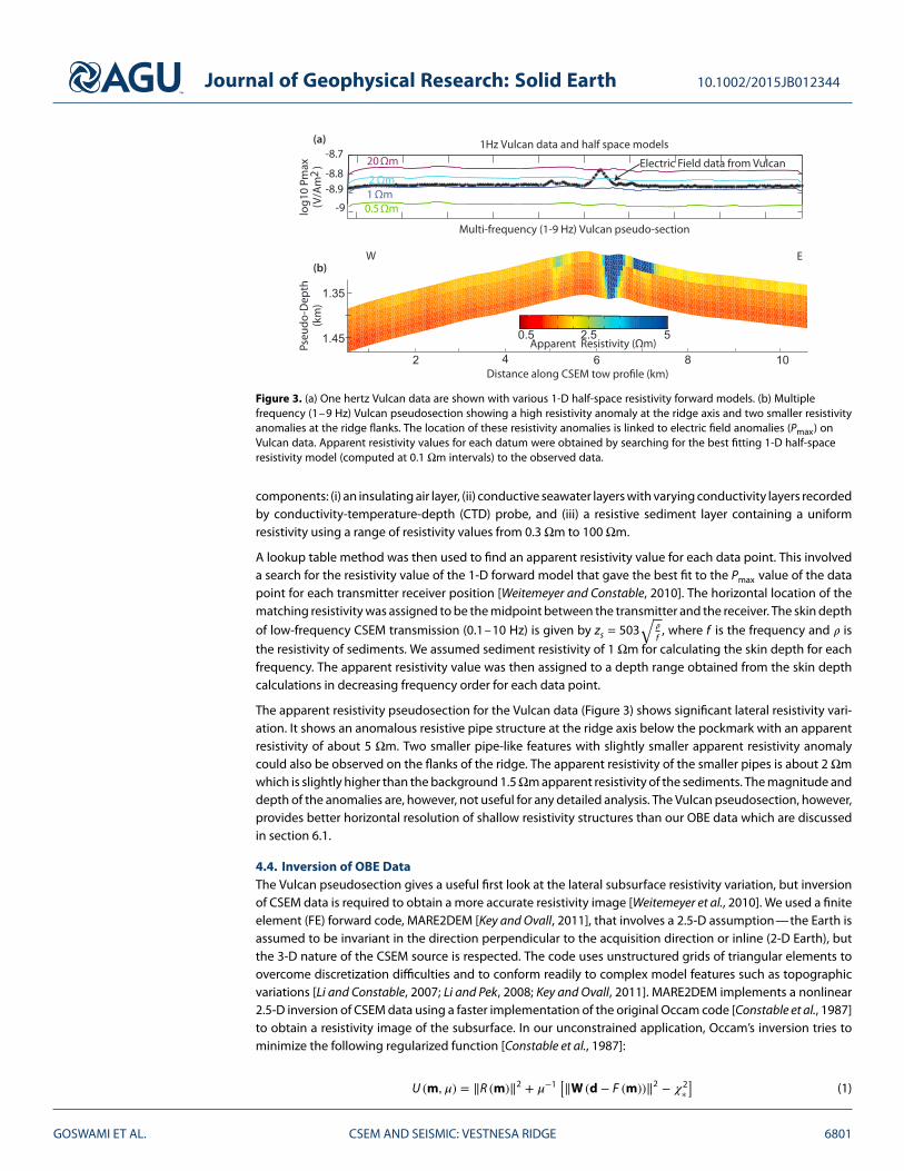
Figure 3. (a) One hertz Vulcan data are shown with various 1-D half-space resistivity forward models. (b) Multiplefrequency (1–9 Hz) Vulcan pseudosection showing a high resistivity anomaly at the ridge axis and two smaller resistivityanomalies at the ridge flanks. The location of these resistivity anomalies is linked to electric field anomalies (Pmax) onVulcan data. Apparent resistivity values for each datum were obtained by searching for the best fitting 1-D half-spaceresistivity model (computed at 0.1 Ωm intervals) to the observed data.

components: (i) an insulating air layer, (ii) conductive seawater layers with varying conductivity layers recordedby conductivity-temperature-depth (CTD) probe, and (iii) a resistive sediment layer containing a uniformresistivity using a range of resistivity values from 0.3 Ωm to 100 Ωm.

A lookup table method was then used to find an apparent resistivity value for each data point. This involveda search for the resistivity value of the 1-D forward model that gave the best fit to the Pmax value of the datapoint for each transmitter receiver position [Weitemeyer and Constable, 2010]. The horizontal location of thematching resistivity was assigned to be the midpoint between the transmitter and the receiver. The skin depth

of low-frequency CSEM transmission (0.1–10 Hz) is given by zs = 503√

𝜌

f, where f is the frequency and 𝜌 is

the resistivity of sediments. We assumed sediment resistivity of 1 Ωm for calculating the skin depth for eachfrequency. The apparent resistivity value was then assigned to a depth range obtained from the skin depthcalculations in decreasing frequency order for each data point.

The apparent resistivity pseudosection for the Vulcan data (Figure 3) shows significant lateral resistivity vari-ation. It shows an anomalous resistive pipe structure at the ridge axis below the pockmark with an apparentresistivity of about 5 Ωm. Two smaller pipe-like features with slightly smaller apparent resistivity anomalycould also be observed on the flanks of the ridge. The apparent resistivity of the smaller pipes is about 2 Ωmwhich is slightly higher than the background 1.5Ωm apparent resistivity of the sediments. The magnitude anddepth of the anomalies are, however, not useful for any detailed analysis. The Vulcan pseudosection, however,provides better horizontal resolution of shallow resistivity structures than our OBE data which are discussedin section 6.1.

4.4. Inversion of OBE DataThe Vulcan pseudosection gives a useful first look at the lateral subsurface resistivity variation, but inversionof CSEM data is required to obtain a more accurate resistivity image [Weitemeyer et al., 2010]. We used a finiteelement (FE) forward code, MARE2DEM [Key and Ovall, 2011], that involves a 2.5-D assumption—the Earth isassumed to be invariant in the direction perpendicular to the acquisition direction or inline (2-D Earth), butthe 3-D nature of the CSEM source is respected. The code uses unstructured grids of triangular elements toovercome discretization difficulties and to conform readily to complex model features such as topographicvariations [Li and Constable, 2007; Li and Pek, 2008; Key and Ovall, 2011]. MARE2DEM implements a nonlinear2.5-D inversion of CSEM data using a faster implementation of the original Occam code [Constable et al., 1987]to obtain a resistivity image of the subsurface. In our unconstrained application, Occam’s inversion tries tominimize the following regularized function [Constable et al., 1987]:

U (m, 𝜇) = ‖R (m)‖2 + 𝜇−1[‖W (d − F (m))‖2 − 𝜒2

∗]

(1)



Table 2. 𝜒2 Misfit for the 2-D VTI Anisotropic Inversion for Individual OBE Sitesand Frequenciesa

OBE Site 1 Hz 3 Hz 5 Hz 7 Hz

V01 0.60 0.42 0.46 0.51

V02 0.64 0.56 0.61 0.68

V03 0.70 0.61 0.56 0.62

V04 0.76 0.68 0.73 0.79

V05 0.79 0.76 0.77 0.83

V06 0.89 0.76 0.77 0.78

V07 0.84 0.74 0.75 0.80

V08 0.85 0.76 0.69 0.77

V09 0.85 0.64 0.63 0.68

All 0.77 0.68 0.67 0.73aInversion target misfit of 0.75 was achieved in eight iterations.

where ‖.‖ is the Euclidean norm and R, the measure of roughness, is the discrete first difference operatoron the model vector m which consists of logarithmic resistivity 𝜌 values. The first term acts as a regularizerto stabilize the inversion and prevents it from producing wildly oscillating resistivity structures [Constableet al., 1987]. The second term is the measure of the misfit of the forward response F(m) to the data d. W isa weighting function that is the inverse of the standard data errors and 𝜒2

∗ is the target misfit. The result ofOccam inversion is mathematically unique because the inversion automatically chooses a value of Lagrange’smultiplier, 𝜇, in order to fit the smoothest model to the data. In the initial stages of the inversion, it triesto minimize the misfit of the model predictions until it reaches the target misfit. Once the target misfit isreached, it performs a search over a range of 𝜇 values to find the smoothest model. The unique smoothmodel is almost independent of the starting model [Wheelock, 2012] in the absence of excessive noise orextreme subsurface resistivity structures.

Two-dimensional inversion of CSEM data requires careful parameterization. Multifrequency (1–7 Hz) OBEamplitude and phase data with transmitter-receiver offsets 850 m to 3000 m were used for the inversion. Wespecified a simple starting model containing a highly resistive air layer (1012Ωm), seawater with 10 horizon-tal resistivity layers (0.295–0.345 Ωm), computed from the recorded CTD measurements during the surveyand a constant resistivity of 1 Ωm for the sediments below the seafloor. We also specified an accurate seafloorbathymetry, using the sum of the altitude (from altimeter) and depth (from CTD) mounted on the DASI frame.The air and seawater resistivity were fixed while the resistivity below the seafloor is a free parameter in theinversion scheme. Beneath the seabed, the initial triangular mesh were set up such that the mesh becamesparser with depth and toward the ends of the profile to minimize computation time. To choose a reason-able target misfit and ensure that the inversion satisfy the global minimum, we ran an initial inversion to anextremely low (0 or 0.1) target misfit, which the inversion could never reach. The target misfit is then found byanalyzing the value of misfit and Lagrange’s multiplier, and the inversion was rerun with the new target misfit.Both isotropic and anisotropic inversions were initially tested and produced very similar models for the giventarget misfit and error structures. Since the Occam inversion optimizes the value of Lagrange’s multiplier andthe roughness term for the given misfit, these parameters are not a good measure of how identical the twomodels are. Therefore, we refer to the visual similarity of the models. The anisotropic inversion with verticaltransverse isotropy (VTI) was, however, smoother in the shallow sediments and converged faster (eight iter-ations) than the isotropic inversion (14 iterations) and was chosen for our analysis. This inversion reached atarget root-mean-square misfit of 0.75 (Table 2) for the given error (approximately 2–3% of the datum).

4.5. OBS Data AnalysisData from the OBS8 deployed on the flank of the ridge were of high quality, and it was straightforward to picka series of reflection events extending 700 ms below the seabed at normal incidence (Figure 4a). Picks weremade mainly on the hydrophone component. However, the hydrophone was saturated by the shots at shortrange and the corresponding artifact obscures reflectors within 50 ms of the direct arrival. Therefore, the firstreflector below the seabed was picked on the vertical geophone component instead. Pick uncertainties varyfrom 4–5 ms near the seabed to 8 ms at the deepest reflector. Data from the OBS5 deployed on the pockmark



Figure 4. (a) Record section from OBS8 on the flank of Vestnesa Ridge. Data were filtered with a trapezoidal band-passfilter with corner frequencies of 10, 20, 250, and 300 Hz and flattened on a direct arrival pick. Hydrophone data areshown at negative offsets and geophone data at positive offsets. Red circles mark every tenth travel time pick.(b) Record section from OBS5 on the pockmark. Processing as for OBS8; hydrophone data only are shown, and redcircles mark every tenth travel time pick. (c) Predicted (black lines) and observed (red circles, subsampled as above)travel times for modeled reflectors. (d) Corresponding velocity model. Inverted triangles mark OBS positions, and blacklines mark picked reflectors.

were much more difficult to interpret (Figure 4b), but several shallow reflectors could be traced between thetwo instruments using data from the 60 m streamer. The deepest of these reflectors is the BSR. Some deeperreflectors could also be identified in these data but could not be correlated confidently with reflectors pickedon OBS8.

A velocity model was developed using the forward modeling code of Zelt and Smith [1992]. Based on CTD data,the ocean layer was assigned a velocity decreasing linearly from 1.48 km/s at the sea surface to 1.465 km/s atthe seabed. Reflector depths were constrained using the coincident reflection profile, and only velocities wereadjusted to fit the OBS data. The two OBSs sample the subsurface in a region about 2 km across at the depthof the BSR, so with 3 km between the OBSs, the experiment is not reversed in the classical sense, and a widerange of models could be constructed that would fit the data. Our preferred model (Figure 4d) was developed



Figure 5. The seismic profile 2012_10 was acquired during the 2012 cruise and shows prominent acoustic signatures ofsubsurface features at the Vestnesa Ridge. The seismic data were poststack time migrated and have been converted todepth using a 1-D velocity function obtained from the OBS data analysis (Figure 8).

by considering each OBS separately and then merging the models. This model has a root-mean-square misfitof 7 ms and a normalized 𝜒2 statistic of 1.485. Given the high quality of the data and pick uncertainties of1–2% of the two-way time of reflections below the seabed, velocity uncertainties in the vicinity of OBS8 arejust a few percent. At OBS5 the uncertainties are larger because of the difficulty of picking reflections.

4.6. Seismic Reflection DataThe seismic reflection data (Figure 5) from the 60-channel streamer were poststack time migrated using aKirchhoff migration and converted to depth using a simple 1-D variation of velocity with depth below theseabed obtained from the OBS data analysis.

5. Synthetic Model Studies of CSEM Data

A resistivity model obtained from the smooth Occam inversion [Constable et al., 1987] usually has poorerresolution compared to seismic velocity models due to the difference in the physics of energy propagation[Constable, 2010]. However, our resistivity model was constrained by nine OBE sites which were approximately500 m apart, whereas the velocity model was obtained from only two OBS stations that were 3 km apart.We, therefore, expect our resistivity model to have better spatial resolution and coverage than our velocitymodel. The resistivity model obtained from Occam inversion eliminates spurious features and retains only theessential features that explain the CSEM data [Constable et al., 1987]. The resistivity solution thus obtained isa unique smooth model [Wheelock, 2012], but no measure of model uncertainty or resolution is available. Weaddress this issue via synthetic studies.

Inline CSEM data are sensitive to transverse resistance, i.e., the product of resistivity of a feature and its thick-ness [Constable, 2010]. The resistivity contrast between a resistive feature and the background sediments istherefore an important consideration in trying to answer questions about resolution and sensitivity of ourCSEM survey. We want to understand the effect of resistivity contrast and variation in fluid composition onresolution of inverted CSEM data. We have attempted to ensure all parameters in the synthetic inversionresemble the real data in terms of available data, acquisition geometry, S/N ratio, and predicted errors. Gaus-sian random noise of 2% was added to the synthetic data before inversion. We assumed an ideal scenariowhere we are able to estimate our errors and specified a 2% data error for the inversion and a target 𝜒2 valueof 1 which indicates that the model fits the data within their uncertainties. It is, however, likely that the realdata have slightly larger uncertainty than we have incorporated in the synthetic data inversions. The syntheticmodel analysis will therefore provide the best-case scenario of what we can sense and resolve using our CSEMexperiment.



We have based our synthetic models primarily on features observed on seismic reflection data (Figure 5). Wetested the sensitivity and resolution of a compaction model and various cases of buried resistors. Our assess-ment of an interpretable anomaly is a resistivity anomaly that has at least the lateral width of two consecutiveelements of our initial grid (≥100 m) and approximately 0.5 Ωm of resistivity contrast.

5.1. Model Generation Using Archie’s EquationWe assumed a pore-filling scenario and applied a modified version of Archie’s equation [Archie, 1942; Winsaueret al., 1952; Hearst et al., 2000] to calculate the approximate subsurface resistivity values for each model. Porewater saturation in sediments can be expressed as

Sw =[𝜌wa𝜙−m

𝜌

] 1n

(2)

for pores partially filled with water and hydrate or gas. Here Sw is sediment water saturation, 𝜌w is the porewater resistivity, 𝜌 is the measured resistivity of sediments, 𝜙 is the sediment porosity, and n is the saturationcoefficient, often equal to the cementation constant, m. The tortuosity constant, a, and cementation con-stant, m, are both related to the interconnection of pores in the sediment matrix. The tortuosity constantwas added to the original Archie’s equation [Archie, 1942] by Winsauer et al. [1952] and should theoreticallybe a = 1. The saturation constant n was introduced later by Hearst et al. [2000] to account for variation inpore shape, connectivity, and the distribution of the conducting phase. SR can easily be calculated from watersaturation using

SR = 1 − Sw (3)

Since we have no empirical values of Archie’s constants for the study area, we used empirical constants fromother studies with similar lithologies; a = 1, m = 2.4, and n = 2 [Archie, 1942; Jackson et al., 1978; Evans et al.,1999; Evans, 2007; Schwalenberg et al., 2010; Weitemeyer et al., 2011]. A pore water resistivity trend with depthwas obtained using the relationship of Becker [1985]

𝜌w = (3 + T∕10)−1 (4)

where T is the sediment temperature in degrees Celsius obtained using bottom water temperature of−0.84∘C(obtained from DASI CTD) and a geothermal gradient of 80 C/km [Vanneste et al., 2005; Geissler et al., 2014].The estimated pore water resistivity trend was similar to the pore water salinity derived pore water resistivityfor nearby Ocean Drilling Program (ODP) Site 986 [Jansen et al., 1996]. Sediment resistivities obtained usingthese assumptions are displayed in Table 3 which show resistivity values for different assumed porosity andpore water saturation which were used for building our synthetic models.

5.2. Simple Compaction ModelA resistivity model representing pore water-saturated sediments with decreasing porosity and pore waterresistivity with depth (Table 3), similar to ODP Site 986 [Jansen et al., 1996], was first tested (Figure 6a). Limi-tations of our model-building tool prevented us from specifying smooth changes in porosity, so we defineda five-layer model, which sufficiently accounts for the porosity changes with depth. The inversion convergedrapidly (five iterations), and the result shows a strong resemblance to the true model in the overall trend andresistivity values (Figure 6b). Since EM wave propagation at low frequency is diffusive [Constable, 2010], andOccam inversion outputs a smooth model, the inversion result does not contain the sharp resistive bound-aries of the true model. Otherwise, the inversion easily recovers the changes in resistivity in the true modeldown to a depth of about 2.5 km. However, the value of resistivity recovered for the 3Ωm resistor is influencedby the 4 Ωm resistivity of the zone beneath.

This observation suggests that we are probably at the limit of resolution of the inversion at the 3–4 Ωmboundary. The maximum depth to which our inversion is sensitive, however, is not simple and depends on theavailable data range, amount of noise, and data errors. An increase in the amount of random noise and spec-ified data uncertainty in inversion parameters both lead to a decrease in sensitivity to the deepest resistivityboundary, and we lose sensitivity to this boundary if noise exceeds 7% of signal in the synthetic inversions.



Table 3. Sediment Resistivity for Varying Pore Water Saturation for an Assumed EffectivePorosity, and Pore Water Resistivity Trend Similar to Site 986 [Jansen et al., 1996]a

Effective Pore Water Pore Water Resistivity AssumedPorosity (%) Resistivity (Ωm) Saturation (%) (Ωm) Depth (m bsf b)

60 0.30 100 1 0–100

95 1.1

90 1.3

80 1.6

50 4.0

48 0.26 100 1.5 100–200

95 1.7

90 1.9

80 2.4

50 6.0

37 0.19 100 2 200–500

95 2.3

90 2.5

80 3.2

50 8.2

26 0.12 100 3 500–1200

95 3.4

90 3.8

80 4.8

50 12.2

19.5 0.08 100 4 1200–2200

95 4.5

90 5

80 6.3

50 16.2aResistivity was calculated using Archie’s equation [Archie, 1942] for a = 1, m = 2.4, and n = 2.bMeters below seafloor.

5.3. Buried Resistors5.3.1. Shallow PipeAn acoustic chimney is observed below the pockmark on seismic reflection data (Figure 5). We designed a800 m wide and 200 m thick resistive pipe which we expect to resolve if there is sufficient resistivity con-trast with the background, as the width of this pipe is more than twice the burial depth [Constable, 2010]. Wetherefore wanted to test the minimum resistivity contrast within the pipe that we can resolve in the inversionof synthetic data (Figure 6d). Assuming that porosity does not vary laterally, we found that a resistivity con-trast equivalent of SR = 5% or higher within the modeled pipe was required to show up as an interpretableanomaly (Figure 6e). The minimum width of a shallow pipe that can be resolved by our inversion was primarilycontrolled by the size of the meshes used for inversion. We were only able to test and resolve pipe anoma-lies wider than 100 m, as the minimum side length of our user-defined triangular mesh in the shallow was50 m. This value was based on the 100 m dipole length and approximately 46 m separation between eachstacked datum.5.3.2. Shallow ResistorA zone of enhanced amplitude reflectors below the ridge axis can be observed on seismic reflection dataaround the base of GHSZ (about 200 m beneath the seabed) (Figure 5). Assuming this enhanced reflectivity isdue to accumulation of free gas [Hustoft et al., 2009; Bünz et al., 2012], we would also expect a resistive anomaly.Whether the anomaly is resolved by our CSEM experiment depends on the amount of resistive material in thepores. To inform us about the minimum saturation of the resistive material in this zone that we could resolve



Figure 6. Inversion of synthetic CSEM data with identical acquisition geometry, data range, and S/N ratio as acquired data, to test sensitivity and resolution of theinversion for various synthetic models. The synthetic study shows (a and b) a simple compaction model, (d and e) a shallow pipe with resistivity contrastequivalent to SR = 5% resistive material; (g and h) a shallow buried resistor with resistivity contrast equivalent to SR = 20% resistive material, and (j and k) a deepresistor with high resistivity contrast (approximately SR = 50%) can be resolved by the CSEM inversion. Note that the color scale is different for Figures 6g and 6h.(c, f, i, and l) Resistivity-depth profiles extracted at 6.3 km model distance (dashed line) are also displayed to the right of each inversion model for each synthetictest. The comparison between true and inverted models demonstrates that the inversion almost recovers the transverse resistance for each synthetic case study.



with our CSEM survey, we generated synthetic models in which a 3 km wide and 80 m thick zone 200 m belowthe ridge axis had SR values of 2%, 5%, 10%, 20%, and 50% (Figure 6g).

The inverted resistivity of the various scenarios suggests that although SR = 10% shows up as a slight anomalyon the inversion results, it will be hard to interpret the result without prior knowledge of the true model.SR = 20% was inferred to be the lower limit for our CSEM survey to resolve confidently (Figure 6h). Althoughwe are able to resolve this SR = 20% resistive anomaly, the dimensions of the resistor are different from thetrue model. There is also an effect on the resistivity of the deeper 3 Ωm resistor due to a possible trade-offbetween the thickness and resistivity of the zone, as CSEM data are sensitive to transverse resistance. For a1-D resistivity profile extracted at 6.3 km model distance (Figure 6i), the transverse resistance of 208 Ωm2 forthe 80 m thick (1450–1530 m), 2.6 Ωm resistor of the true model was recovered by the CSEM inversion as a100 m thick (1440–1540 m) resistor with resistivity ranging in 1.8–2.3 Ωm.5.3.3. Deeper ResistorWe would like to determine whether there is any deep gas reservoir feeding the observed fluid escape featureson seismic reflection data. The maximum resolvable depth of the CSEM inversion is around 2.5 km (about 1 kmbeneath the seabed) (Figure 6b). We therefore wanted to see whether we can resolve the top and the base ofa 120 m thick deep resistive feature of 12 Ωm at a depth of approximately 2.2 km (Figure 6j).

We found that a very high resistivity contrast was required for the inversion to resolve such a deep resis-tor; e.g., our SR = 50% saturation model. The true resistivity anomaly modeled was 12 Ωm extended from4.5 to 8.2 km along the profile and was 120 m thick. The inverted resistivity anomaly was about 2–3 times(240–360 m) the original thickness and slightly shorter (around 500 m) with lower resistivities between 4 and6 Ωm in magnitude. The inverted deep resistive anomaly also distorted the deeper layers of the model andintroduced a deep terminating layer. The CSEM inversion is at the limits of its sensitivity at the center of ourdeep synthetic anomaly around 2.2 km. It therefore fails to fully resolve the base of the deep anomaly as wellas the deeper resistive boundary underneath the anomaly as it tries to find a trade-off between resistivity andthickness to account for the anomaly in the synthetic data (Figure 6k). The transverse resistance of 1440 Ωm2

(120 m × 12 Ωm) for the deep resistor between 2120 and 2240 m was recovered as 1426 Ωm2 by integrat-ing the transverse resistance between 1980 and 2260 m (280 m thick) which had resistivities between 3.7 and5.9 Ωm (Figure 6l). The transverse resistance of the inverted model for the deep resistor was within 1% of thetrue model.

6. Result6.1. Two-Dimensional InversionThe resistivity models obtained from the isotropic inversion (Figure 7a) and VTI anisotropic inversion(Figures 7b to 7d) of OBE data were very similar, with the vertical resistivity model (Figure 7b) being smootherfor the shallow sediments. Very weak anisotropy within the shallow sediments (Figure 7d) was predicted bythe anisotropic inversion. However, in deep water setting like our survey (>1200 m), inline data are primarilysensitive to vertical resistivity [Ramananjaona et al., 2011; MacGregor and Tomlinson, 2014]. Additionally, Mac-Gregor and Tomlinson [2014] and Ramananjaona et al. [2011] also showed that broadside data are requiredto have improved sensitivity to the horizontal resistivity in deep waters. However, for our data, between theoffsets (850–3000 m) and frequencies (1–7 Hz) used in our inversion, inline data could have some sensitiv-ity to horizontal resistivity as well [MacGregor and Tomlinson, 2014]. Since only inline data were available forour inversion and the vertical and horizontal resistivity models were very similar, we will focus on the verticalresistivity results in this paper. The main features of the vertical resistivity model are discussed below.6.1.1. Central Resistive PipeA high-resistivity zone can be observed beneath the seafloor pockmark from 6.1 to 6.6 km along the resistiv-ity profile, coinciding with the pipe structures imaged in the seismic reflection profile (Figure 7b). This zoneextends from the seafloor to a depth of about 300 m below the pockmark. It has slightly higher resistivity valuetoward the center, which increases in magnitude to the seafloor. The resistivity ranges from about 2.5 Ωm atthe edges to about 4 Ωm at center in the lower part of the pipe whereas the central part of the anomaly isabout 6 Ωm just below the pockmark location. The feature is also connected to a deeper zone of high resis-tivity via an extension of the elevated resistivity pipe of about 2.25 Ωm magnitude. The core of the higherresistivity appears to be located around 5–7 km along the profile at the depth of about 2.3 km below the seasurface (approximately 1.3 km below seafloor) with a maximum resistivity of approximately 3 Ωm.



Figure 7. Resistivity models obtained from 2.5-D inversion of OBE data. (a) Isotropic inversion was initially tested andshows a similar result to the anisotropic inversions. The isotropic inversion reached the target misfit of 0.75 in 14iterations. (b) The vertical resistivity model obtained from the VTI anisotropic inversion results are, however, smootherjust beneath the seafloor and was therefore chosen as the preferred result for interpretation. The anisotropic inversionreached the target misfit of 0.75 in eight iterations. (c) The horizontal resistivity model also shows lateral resistivityvariation with a prominent central chimney structure with a zone of high resistivity at depth. (d) The ratio of vertical tohorizontal resistivity reveals weak anisotropy in the shallow sediments.

6.1.2. Narrow Elevated Resistive Zones at Ridge FlanksA few regions of higher resistivity connected to the deep resistive anomaly can be observed on both flanks ofthe ridge (Figure 7b). These features of about 2.25 Ωm and sometimes can be observed to reach close to theseafloor, such as at around 5 and 7 km along the model distance (Figure 7b).

6.2. Velocity ModelsAt OBS8, the model shows velocities increasing with depth from 1.51 km/s at the seabed to 1.88 km/s at theBSR, then a decrease to 1.70 km/s, with anomalously low velocities then present to the bottom of the model

Figure 8. Solid line marks velocity at the locationof OBS8. Dashed line marks velocity at site N3 ofChabert et al. [2011]. Thin curve marks Hamilton’s[1980] regression for terriginous sediments.

(Figures 4d and 8). The model includes lateral velocity varia-tions in all the layers, but an adequate fit to the data can beachieved if such variations are restricted to the layer immedi-ately above the BSR. Larger lateral variations in the shallowerlayers are also allowed by the data from OBS5, and such vari-ations might not be sampled by OBS8 since reflection pointsfor shallow reflectors are very close to the OBS.

The lateral velocity increase can be attributed to the presenceof hydrate beneath the pockmark, but its magnitude is notsufficiently constrained to allow an estimate of hydrate satu-ration based on these data alone. The spatial coverage of thevelocity model (Figure 4d) is limited by the number of OBSstations and their large separation (approximately 3 km).

7. Discussion

Reliable coincident seismic and resistivity models are limitedto a small area (Figure 9a) due to large spacing (approximately3 km) between the two OBSs and extend only up to a depthof 1850 m, which limits the maximum depth of our joint inter-pretation. A low-velocity zone can be associated with the



Figure 9. (a) Seismic velocity and seismic reflection data overlay shows a low-velocity zone associated with theenhanced reflectors beneath the GHSZ. (b) Vertical resistivity and seismic reflection data overlay shows a highcorrelation between the resistive chimney and the acoustic chimney. The seismic fluid escape features on the ridgeflanks are also associated with higher resistivity anomalies. No strong resistivity anomaly can be observed with thehigh-amplitude reflectors beneath the BSR. (c) Velocity contours overlaid on resistivity results show an increase inseismic velocity toward the lateral position of the resistive chimney. There is no clear resistivity anomaly associated withthe low-velocity zone beneath the BSR at the ridge axis suggesting a very low concentration of free gas.

enhanced amplitude reflectors beneath the GHSZ with lower apparent frequency (Figure 9a). The frequencyloss and enhanced amplitudes can be caused by the presence of gas [Hustoft et al., 2007]. The low-velocityzone suggests the presence of a free gas zone (FGZ) at least 50 m thick below the ridge axis. The FGZ mayextend at least 300 m below the BSR (Figure 8), but its thickness is not constrained by our OBS data on theridge axis.

The zone directly above the FGZ has high velocity (Figure 9a). In order to assess the presence of velocity (andresistivity) anomalies due to the presence of hydrate or gas, we must establish a reference background velocityfunction that we expect in the absence of either.

7.1. Velocity AnomalyThe appropriate background velocity for hemipelagic sediments in this region was investigated extensivelyby Westbrook et al. [2008], using differential effective medium (DEM) models. They concluded that two alter-native models (their DEM2 and DEM3) were most appropriate, and these models both predict a very similarvelocity-depth function to the empirical curve of Hamilton [1980] (Figure 8). We constructed velocity anomaly



Figure 10. Background porosity estimate for the studyobtained using a reference velocity function. Thereference velocity function consists of Hamilton’s [1980]curve for terrigeneous sediments for the top 800 m bsfand Ritzmann’s [2004] velocity trend below. It wasconverted to density and porosity using Hamilton’s[1978] regression equations. A different velocity-densityequation (equation (4)) was used for the unconsolidatedsediments (≤ 2 km/s). Archie’s equation [Archie, 1942](empirical constants a = 1, m = 2.4, and n = 2) was usedto convert the reference porosity function into abackground resistivity function.

plots using DEM2, DEM3, and Hamilton’s curve as refer-ence velocity, and all looked very similar; therefore, wehave used the Hamilton’s curve here (Figure 11a).

We observe a positive velocity anomaly above the BSRassociated with our high-velocity zone and a nega-tive velocity anomaly associated with the underlyingFGZ (Figure 11a). Similar observations of high-velocityanomalies above the BSR and low-velocity anoma-lies beneath have been reported due to gas hydratenear our study area, on the West Svalbard margin[Westbrook et al., 2008; Hustoft et al., 2009; Chabertet al., 2011] and on the mid-Norwegian Atlanticmargin [Bünz, 2004; Hustoft et al., 2007; Plaza-Faverolaet al., 2010].

7.2. Resistivity AnomalyIn the absence of hydrate or gas, the seismic veloc-ity response in the subsurface is largely controlled bychanges in porosity whereas resistivity changes can becaused by changes in either porosity or fluid compo-sition. Assuming water-saturated pores, we used thereference background velocity trend to calculate a ref-erence background porosity trend (Figure 10). First, weextended the reference velocity function beyond 1 kmdepth below the seabed, where the comparisons ofWestbrook et al. [2008] are no longer valid, by usingthe velocity trend of Ritzmann et al. [2004]. Initially,we used Hamilton’s [1978] velocity-density relation-ship to convert the reference velocity function to areference density function. However, we found thatHamilton’s [1978] relationship for unconsolidated sed-iments (velocity <2 km/s) provided a poor fit to thedensity log from nearby ODP Site 986 [Jansen et al.,1996] which likely sampled similar lithologies. There-fore, we used an altered equation for the unconsoli-dated sediments which provided a good fit to densityand porosity data from Site 986 (Figure 10).

d = 0.743V + 0.602 (5)

Here d is the density and V is the P wave velocity of sediments. The altered equation also provided a better fitthan Hamilton’s [1978] relationship to the Site 986 density log when we used both relationships to convert theODP velocity log to density. We used a grain density of 2710 kg/m3 and pore water density of 1023.7 kg/m3

[Jansen et al., 1996] to obtain a reference porosity trend. Comparison of our reference velocity to the ODPSite 986 velocity log suggests approximately 4% uncertainty in our reference velocity function within the top1000 m bsf. We infer approximately 5% uncertainty in our estimated density obtained using equation (5) bycomparison with the Site 986 density log and 6–8% uncertainty in our inferred porosity trend.

The background resistivity trend was then estimated using Archie’s equation [Archie, 1942] using a = 1 andn = 2 and m = 2.4, which fits the ODP Site 986 resistivity log. The pore water resistivity trend was derivedfor the synthetic models and matches the trend suggested by ODP Site 986 salinity [Jansen et al., 1996]. Theresistivity anomaly (Figure 11b) was calculated by comparing the vertical resistivity model (Figure 7b) withthe reference background resistivity model. Reference resistivity obtained from porosity using equation (2)also suggested a reasonable fit to the ODP Site 986 resistivity log for m = 2.2–2.6. Accounting an uncertaintyof 10% for Archie’s constant m and 10–15 % for the geothermal gradient [Vanneste et al., 2005] in equation(4), roughly 18–20% ambiguity is likely for our reference resistivity trend.



A resistivity anomaly straddling the BSR (Figure 11b) can be associated with the velocity anomalies (Figure 11a)beneath the ridge axis. This display highlights strong anomalies around the chimney structures which extendsbeneath the BSR at the central chimney. The FGZ beneath the ridge axis could be a possible explanation forthe observed negative velocity anomaly and positive resistivity anomaly beneath the BSR, but the positiveresistivity anomaly could also be a smoothing artifact of the CSEM inversion. A joint saturation estimate istherefore not appropriate. Away from the chimney, the free gas saturation immediately below the BSR is likelyto be on the lower end of that predicted at site N3 [Chabert et al., 2011] as indicated by the less pronouncedlow-velocity zone (Figure 8).

There is no strong resistivity anomaly within the GHSZ away from the chimneys, which suggests low hydratesaturations that may not be detectable our survey setup. Hustoft et al. [2009] suggest around 10% hydratesaturation near the base of the GHSZ and around 2% free gas saturation beneath, which is too low to beresolved by our CSEM survey according to our synthetic model studies. A deeper resistivity anomaly can alsobe identified (Figure 11b), which could be caused by widespread presence of free gas beneath the GHSZ witha possible free gas reservoir at depth. At this depth, our data are mainly sensitive to the transverse resistance(Figure 6h) which makes it difficult to perform a saturation analysis.

7.3. Apparent Porosity AnomalyOne common parameter that links resistivity and velocity of sediments is porosity. The velocity and resistivitymodels were converted into apparent porosity models using methods described earlier and compared tothe reference background porosity (Figure 10) function to obtain apparent porosity anomalies. The positivevelocity anomalies above the BSR (Figure 11a) correspond to lower apparent porosity (Figure 11c), and thenegative velocity anomalies beneath the BSR (Figure 11a) correspond to higher apparent porosity (Figure 11c).On the other hand, from resistivity models, we obtain a lower apparent porosity anomalies both above andbeneath the BSR (Figure 11d) since both hydrate and gas show up as positive resistivity anomaly (Figure 11b).

7.4. Chimney StructuresThe central chimney beneath the pockmark is 500–600 m wide whereas the chimneys on the ridge flanksare narrower (100–120 m) with lower resistivity (Figure 9b). The disturbed sequence of reflectors within theacoustic chimneys, and the associated high resistivity extend beyond the FGZ beneath the BSR (Figure 9b).This observation could suggest a deeper source of fluid migration into the GHSZ.

Geochemical analysis of samples taken at the pockmark above the central chimney suggests episodicrelease of thermogenic gas through the chimney for over 20 ka [Panieri et al., 2014; Smith et al., 2014a]. Thecentral chimney is therefore likely a long-term feature with three-phase equilibrium for gas, hydrate, and waterextending throughout the GHSZ [Liu and Flemings, 2007; Smith et al., 2014b]. We therefore expect both gasand hydrate to coexist within the chimney.

Free gas migration through the long-term chimney is likely to occur through microfractures and faults [Smithet al., 2014b] which are not resolved by our seismic reflection data. However, the enhanced reflectors asso-ciated with the FGZ beneath the central chimney have a small vertical offset between the eastern and thewestern ridge flank, which is an argument for possible faulting within the central chimney. Microfracturesand faults within a fluid escape chimney with similar sediments have been suggested at the Nyegga CNE03pockmark [Plaza-Faverola et al., 2010].

7.5. Free Gas and Hydrate Saturation Estimates Within the GHSZBy including both resistivity and velocity information in rock physics models, we can constrain both free gasand hydrate saturations within the GHSZ. Our pore water-saturated background velocity and resistivity mod-els were based on ODP Site 986 [Jansen et al., 1996] and may not be accurate as this site is around 200 kmaway from our study area. Therefore, for quantitative saturation estimates, we computed a depth-integrated,average velocity and resistivity for the top (0–100 m bsf ) and bottom (100 m bsf to BSR) parts of the GHSZ forevery 50 m along our profile (Figures 11e and 11f). This approach has the additional benefit of reducing theamount of scatter in our cross plots when comparing our data to predicted resistivity and velocity models.The observed depth-integrated average velocity for the top (Figure 11e) and bottom (Figure 11f ) parts of thechimney was around 5% and 8% higher than the background, respectively. The observed depth-integratedaverage velocity outside the chimney was similar to the background for the top part of the GHSZ (Figure 11e)and around 2% higher for the bottom part of the GHSZ (Figure 11f ). In addition to the velocity anomalies,the observed depth-integrated average resistivities within the central chimney were 15–380% and 30–180%



Figure 11. (a) Velocity anomaly showing the difference between the observed velocity model and a water-saturated background velocity obtained from theHamilton [1980] curve for terrigenous sediments. A positive anomaly within the GHSZ and a negative anomaly beneath the GHSZ can be observed clearly.(b) Resistivity anomaly showing the difference between the observed resistivity and background resistivity generated from velocity-derived porosity (Figure 10)highlights anomalies associated with the chimney structures and at depth. (c) Apparent porosity anomaly derived from the velocity model showing a region oflower apparent porosity above the BSR and higher apparent porosity below the BSR. (d) Apparent porosity anomaly derived from the resistivity model showing aregion of lower apparent porosity associated with the chimney structures beneath the GHSZ. Depth-averaged velocity and resistivity comparison for the (e) toppart and (f ) bottom part of the GHSZ along the CSEM profile showing the locations of the highest anomalies. A coincident positive resistivity and positivevelocity anomaly can be observed around the central chimney.



higher than the background for the top (Figure 11e) and bottom (Figure 11f ) parts, respectively. Outside thecentral chimney, the depth-integrated average resistivities for the top (Figure 11e) and bottom (Figure 11f )parts of the GHSZ were 0–300% and 30–300% higher than the background, respectively. To quantify theamount of hydrate and free gas saturation within the top and bottom parts of the GHSZ, we replaced the porewater in our background models by varying amounts of hydrate and gas to estimate the theoretical velocityand resistivity responses.7.5.1. Velocity ModelsWe used two different rock physics models for calculating the velocity response due to change in porefluid saturation: fracture-filling model of Plaza-Faverola et al. [2010] and Gassman’s fluid substitution[Berryman, 1999].

1. We used the simple fracture-filling model of Plaza-Faverola et al. [2010] as our preferred model for estimat-ing the velocity response due to varying hydrate saturation within the pores. In this model, free gas replacespore fluids, and hydrate formation from this gas leads to a change in porosity of the original frame. Thismodel, however, only accounts for hydrate as fraction of volume and was not useful for modeling the effectof free gas.

2. To estimate the velocity response for both free gas and hydrate in pores, we adapted Gassman’s fluid sub-stitution [Berryman, 1999] to account for hydrate in the rock frame (see Appendix D). The velocity responseobtained from Gassman’s substitution [Berryman, 1999] is strongly influenced by the mixing model used tocalculate the bulk modulus of the fluid mixture. The Reuss and Voigt bounds provide the lower and upperbound for the bulk modulus, respectively. The Reuss bound is expected to provide an accurate estimateof bulk moduli of the fluid mixture when the constituents are liquids or gases [Mavko et al., 2009] whichleads to a uniform mixture. The effect of nonuniform distribution was modeled by using the Voigt-Reuss-Hillaverage [Mavko et al., 2009].

7.5.2. Resistivity ModelSince we do not have direct measurements of the electrical properties of the various minerals, we usedArchie’s equation [Archie, 1942] for our resistivity calculations. A depth-averaged pore fluid resistivity, adepth-averaged GHSZ porosity, and other empirical constants as used for the background resistivity calcula-tions were assumed. The bulk modulus estimated using Reuss bound and resistivity obtained from Archie’sequation are consistent in the assumption of a uniform fluid distribution (Figures 12a and 12b).7.5.3. Saturation Estimate for Central ChimneyEstimated saturations depend on whether a uniform (Reuss bound) or a nonuniform (Reuss-Voigt-Hill aver-age) fluid distribution is assumed within the pores. Inferred hydrate and free gas saturations for the top(Figures 12a and 12b) and bottom (Figures 12c and 12d) parts of the chimney for each of the mixing modelsare listed in Table 4.

Assuming a nonuniform fluid distribution, up to 22% free gas saturation is inferred at the top part of thechimney (Figure 12b). As the distribution of gas that has migrated through the chimney is likely to be patchy,the nonuniform model (Figures 12b and 12d) is better suited for predicting the effect of the gas on seismicvelocity. So the larger concentrations of gas and smaller concentrations of hydrate predicted from this model,compared with those from the uniform model, are more probable. This high free gas saturation may result inhigh pore fluid pressures that could push fluids, including free gas, to the seafloor [Westbrook et al., 2009].

In the absence of direct sampling of hydrate and gas from deep boreholes in the study area, the inferredhydrate, and gas saturation for the chimney can be compared with those modeled for the postbreaching case(20 ka) of a long-term chimney by Smith et al. [2014b] where 50–80% hydrate and up to 1% free gas saturationwas predicted in the top 200 m. Our saturation estimates are therefore comparable to the model chimney[Smith et al., 2014b] for hydrates but higher for free higher saturation. The model chimney is in similar waterdepths but has a thicker GHSZ and higher temperature and salinity profiles. The 20 ka postbreaching modelof Smith et al. [2014b] suggests highest hydrate and gas saturation directly beneath the seafloor, consistentwith the location of the highest resistivity observed in our model (Figure 9b).

Although we infer the greatest amount of resistive material at the top part of our studied chimney, the hydratesaturation is estimated to be slightly higher at the bottom part of the chimney in the case of our nonuniformfluid distribution, which contrasts with Smith et al.’s [2014b] model. It is difficult to determine the cause ofthe difference between the model chimney and our observations in the absence of temperature and salinitymeasurements from the Vestnesa chimney. If, however, an average salinity of 85 parts per thousand (ppt) and65 ppt was assumed for the top and bottom parts of our chimney, respectively, based on the salinity profile of



Figure 12. Cross plot showing depth-averaged velocity and resistivity for the GHSZ (also see Figures 11e and 11f ) against theoretical models. The resistivity iscalculated using Archie’s equation [Archie, 1942], whereas two different models were used for the velocity: (a) 𝜙 = 55%, (c) 𝜌w = 0.303 Ωm and (b) 𝜙 = 50.5%,(d) 𝜌w = 0.243 Ωm. The Plaza-Faverola et al. [2010] model (solid blue line in each panel) assumes that hydrate is formed as free gas flows into fractures and veinsand alters the porosity of the frame. This model is only valid in the absence of free gas. To model free gas along with hydrate, Gassman’s substitution [Berryman,1999] was used for each load-bearing hydrate frame. The bulk modulus of the gas and pore water mixture was calculated using the Reuss bound (Figures 12aand 12b) and the Voigt-Reuss-Hill average (Figures 12c and 12d) to explore the different fluid mixing scenarios. The noncircled datum represents the regionoutside the chimney.

Smith et al. [2014b], the estimated pore water resistivity using the equation of state of Lewis and Perkin [1981]would be 0.10 Ωm and 0.14 Ωm, respectively. These pore water resistivity values are much lower comparedto 0.30 Ωm (32 ppt) for the top and 0.24 Ωm (30 ppt) for the bottom parts of the chimney estimated for ourarea on the basis of the bottom water temperatures and geothermal gradients (see section 5.1). The amountof hydrate and gas would then be higher in the top part of the chimney for both uniform and nonuniformfluid distribution (Figure E1 in Appendix E). The location of the highest saturation at the top of the chimney isthen consistent with the model of Smith et al. [2014b].7.5.4. Saturation Estimate Outside Central ChimneyOur resistivity and velocity cross plots suggest the presence of up to 30% hydrate saturation in the top partand 20–30% in the bottom part of the GHSZ. Both uniform and nonuniform fluid distribution models suggestless than 5% free gas saturation for the GHSZ with a slightly higher value for the nonuniform model. Whetherwe assume the uniform distribution (Reuss bound) or nonuniform distribution (Voigt-Reuss-Hill average), thepredicted hydrate saturation outside the chimney (Table 4) is higher than previous estimates of 11% for theVestnesa Ridge [Hustoft et al., 2009]. These predictions are closer to those from the frame-plus-pore model ofWestbrook et al. [2008], for their NW Svalbard study location, where 5–25% hydrate in pore space was pre-dicted using a reference velocity from Hamilton [1978]. Our higher hydrate saturation estimates outside thechimney arise from the constraints provided by the resistivity data which allow us to take account of the effectof free gas on velocity within the GHSZ.



Table 4. Inferred Hydrate and Gas Saturation (% of Pore Space) for the Central ChimneyObtained Using Joint Resistivity and Velocity Analysis (Figure 12)a

Uniform (Reuss) Patchy (Voigt)Location Hydrate Gas Hydrate Gas

Chimney Top (0–100 m bsf)

Edge 10–30 <1 10–30 0–2

Center 50–73 1–4 40–52 10–22

Outside 0–30 0–1 0–25 0–4

Bottom (100 m bsf—BSR)

Edge 30–45 <1 30–42 0–5

Center 50–68 0–2 40–55 5–15

Outside 20–30 0–1 20–30 1–3aApproximately ±25% uncertainty is estimates for these inferred saturations.

7.5.5. Saturation UncertaintiesOur inferred saturations have large uncertainties due to assumptions made while choosing the backgroundfunctions and using ODP Site 986 for reference, which is approximately 200 km away. An additional complica-tion for our models is that the host sediments are clay rich which is not accounted for by the modified Archie’sequation (equation (2)) [Archie, 1942]. The effect of clay conductivity and cation exchange capacity [Waxmanand Smits, 1968; Revil et al., 1998] is therefore ignored in our estimates, which likely leads to an overestimateof pore water saturations (Sw). This will lead to an underestimate of hydrate and gas saturations. In addition,hydrate is likely to form in fractures in low permeability clay-rich sediments [Liu and Flemings, 2007], whichour resistivity models do not incorporate.

Perturbation analysis allows us to obtain a first-order estimate of our inferred saturation uncertainties. It is ourpreferred approach due to the nonlinearity in the relationship between velocity, resistivity, and saturation pre-sented in our cross plots (Figure 12). On the basis of analysis of the ODP Site 986 logs, around 4% uncertaintyin our reference velocity and around 10% in our choice of Archie’s parameter m were inferred. The uncertaintyin our reference velocity leads to around 8% uncertainty in our reference porosity used for the saturation esti-mates. Although the depth-averaging approach reduces these uncertainties slightly, we consider the highervalues for our analysis to compensate for the poor controls on our parameter assumptions. The perturbationanalysis for m and porosity suggests up to 18% uncertainty in our inferred saturations of gas and hydratefor both uniform and nonuniform gas distributions. On the other hand, the uncertainty in inferred satura-tion is around 20% due to the difference in assumption of uniform and nonuniform gas distribution models.We therefore assume 20% (larger of the two estimates) as the saturation uncertainty due to ambiguity in theestimated theoretical velocity and resistivity responses. However, no measure of uncertainty in our resistiv-ity data is known. Occam inversion [Constable et al., 1987] only outputs a smooth resistivity model and doesnot provide any measure of model uncertainty. Postcalculation of model uncertainty by perturbing the finalmodel is not practical due to large compute times (current inversion takes approximately 24 h on 64 nodes of4x Xeon E5/Core i7 1333 MHz processors with 256GB RAM) as this would require several inversions to performthis analysis. However, we can infer an uncertainty of 10% in our depth-averaged resistivity and velocity data.This may account for an additional 5% saturation uncertainty. Accounting for the largest errors in the theoret-ical and observed values, we suggest around 20–25% uncertainty in our inferred saturations obtained fromour cross plots.

The inferred values of hydrate and free gas saturation are high for normal values of salinity and even higherfor the values of salinity predicted by Smith et al. [2014b]. The absence of particularly high or low values ofseismic velocity is a consequence of the presence of free gas and hydrate together, probably as a consequenceof locally high pore water salinity caused by the formation of hydrate, which suppresses the conversion of theremaining gas to hydrate. Additionally, the presence of authigenic carbonate, formed by anaerobic oxidationof methane, at shallow depth, would with its high seismic velocity counteract the effect of gas on averagevelocity. As carbonate also has a high resistivity, it cannot be distinguished from hydrate, using our data, soit is probable that in the shallowest part of the chimney, where carbonate is most likely to be abundant, theamount of hydrate is overestimated.



Figure 13. A schematic cartoon of the gas hydrate system at the Vestnesa Ridge on the basis of colocated seismic and CSEM data. A GHSZ with up to 30%hydrate saturation is inferred within the GHSZ on the basis of coincident seismic and resistivity data. Extremely high hydrate and free gas saturation is inferredwithin the chimney beneath the pockmark at the ridge axis where active venting was observed in 2008 [Westbrook et al., 2009]. A FGZ with around 2% free gassaturation is inferred beneath the GHSZ which is likely to be overpressured beneath the ridge axis [Hustoft et al., 2009]. Up to 50% free gas saturation may beinferred directly beneath the chimney using our resistivity estimates. There is also evidence of the FGZ being fed by a deeper gas reservoir.

The presence of hydrate, carbonate, and free gas with high contrasts of acoustic impedance between themand the normal sediment, and the acoustic absorption caused by free gas would lead to significant atten-uation of seismic waves traveling through a volume of sediment that was heavily invaded by them. Strongseismic attenuation beneath the pockmark, however, is not shown above the BSR by seismic reflectionsections, except very locally, although the gas-invaded region beneath the BSR shows strong attenuation(Figure 5). Furthermore, at the seabed, emissions of gas bubbles into the water are confined to a few smallseep sites around the periphery of the pockmark. From these observations, we infer that although highsalinity water is likely to be present locally in and around active gas-migration pathways, it is probably notcharacteristic of the whole of the chimney volume.

8. ConclusionWe were able to constrain the degree of hydrate and free gas saturation within the GHSZ at the Vestnesa Ridge(Figure 13) for the first time, using joint velocity and resistivity analysis from coincident seismic and CSEM data.Although it is difficult to judge the accuracy of these estimates, Gao et al. [2012] showed that joint seismic andresistivity estimates provide better constraints on porosity and fluid saturation compared to estimates usingseismic and EM data individually. From these estimates, we conclude that

1. The top part of the chimney (0–100 m bsf ) beneath the pockmark is likely to be highly saturated by hydrateand gas. Maximum depth-averaged saturations of 73% hydrate and 4% free gas or 52% hydrate and 22%free gas are possible assuming uniform and nonuniform fluid distribution, respectively.

2. In the bottom part of the chimney (100 m bsf—BSR), a maximum depth-averaged saturation of 68% hydrateand 2% free gas or 55% hydrate and 15% free gas are possible assuming uniform and nonuniform fluiddistribution, respectively.

3. Up to 25% hydrate and 2% free gas might be present in the GHSZ outside the central chimney, with highesthydrate saturation in the bottom part of the GHSZ.

4. The amount of gas estimated in the top part of the chimney makes it very likely to be overpressured,resulting in free gas being expelled through the seafloor.

5. Widespread existence of free gas beneath the GHSZ can be inferred, with a possible free gas reservoir atdepth feeding the GHSZ. New CSEM and seismic surveys that have an increased depth of investigationwould be required to resolve fully the size and nature of the deep gas reservoir.



Although there is a need for boreholes into the pockmark and the ridge flank to test our interpretations, wehave been able to demonstrate that CSEM is a good complement to other geophysical methods for resolvingissues of fluid saturation in complex geological settings, such as the Vestnesa pockmark.

Appendix A: NavigationAccurate navigation is essential for improvement in quality of quantitative interpretation using CSEM data[Morten et al., 2009; Constable, 2010; Weitemeyer and Constable, 2014]. Ambiguity in antenna dip and cross-lineuncertainty as a result of feather has large impact on the quality of CSEM inversion [Weitemeyer and Constable,2014]. The GPS provided the ship’s position that was then used as an input to the USBL navigation system toobtain the position of the towed instrument, DASI frame, and HyBIS. The course over ground (COG) of the DASIframe was calculated using the vector given by the instantaneous position of the ship and the DASI frame.We assumed that Vulcan followed the DASI track. The positions of the DASI and Vulcan antennae were thencalculated by back projecting the DASI frame coordinates using the COG and laybacks (Figure 2). Uncertaintiesin position resulting from this approach would affect the accuracy of our CSEM models and were taken intoconsideration in CSEM inversion parameterization (see section 4.2).

Appendix B: Location UncertaintyThe ship’s position obtained from the GPS, which was used by the USBL for the position of the deep towedDASI frame and HyBIS (for OBE deployments), had a horizontal uncertainty of ±4 m. The USBL system wascalibrated during the 2012 cruise and was found to be accurate to 0.1% of slant range. During CSEM operation,the ship maintained a steady course and sailed in an almost straight line. Considering the amount of cable(>1500 m) and the weight of the towed equipment—DASI frame, DASI streamer, and Vulcan—we expectedthem to follow the ship’s track. However, it was found that the position of the DASI frame shifted from slightlynorth of the ship track to slightly south of the ship track around the crest of the Vestnesa Ridge. This could bedue to deepwater currents on the flanks of the ridge.

Although the neutrally buoyant oil-filled streamer used for the DASI antenna was expected to keep it horizon-tal, uncertainty existed over its dip during periods when the length of the tow cable was altered to maintain aconstant height of DASI 50 m above the seabed. The dip and azimuth of the DASI antenna could also have beenaffected by the positive buoyancy of Vulcan, attached to the tail of the antenna by a tow rope. Near-bottomcurrents could also influence the position of DASI antenna and Vulcan. An approximate uncertainty of ±2–3∘

on antenna dip was assumed on the basis of observed jitter on DASI height and changes in bathymetry. Wealso assumed a ±2–3∘ uncertainty in the calculated azimuth of the towed antenna and Vulcan, on the basisof observed jitter in the position of ship and DASI. This orientation uncertainty leads to a±7 m uncertainty forthe DASI antenna-middle position, a ±5 m uncertainty in the DASI antenna-middle depth, and about ±12 muncertainty on the position of Vulcan. The OBE receivers, which were deployed using HyBIS, also had a ±6 mposition uncertainty, on the basis of GPS uncertainty and USBL uncertainty.

Appendix C: Environmental UncertaintyThere were a number of other possible causes of error in our data, such as currents and acoustic interfer-ence, which we grouped as environmental noise. These sources caused a certain amount of instability to ourreceivers during operation and resulted in noise appearing in our data. Stacking of the data into 60 s windowsprovided us with a measure of variance (typically<1.5% of the datum) in our data along with an improvementin S/N ratio.

Appendix D: Estimating Velocity Due to Both Free Gas and HydrateThe reference background P wave velocity and background porosity trends for the study area were presentedin sections 7.1 and 7.2. The shear wave velocity trend was calculated using Castagna’s (1985) mudrock relation[Mavko et al., 2009]. These background trends were then used to calculate the depth-integrated backgroundporosity (𝜙), P wave velocity (vp), and S wave velocity (vs) for the top (0–100 m bsf ) and bottom (101 m bsfto BSR) parts of the GHSZ. The bulk modulus (K), shear modulus (𝜇), and density (d) of hydrate (hyd), gas (g),water (water), and sediment grains (grain) used for the calculations were based on ODP Site 986 (Appendix Dand Table D1) [Jansen et al., 1996; Carcione et al., 2005]. The density of the top and bottom parts of the GHSZwas then calculated from

dGHSZ = (𝜙)dwater + (1 − 𝜙)dgrain (D1)



Table D1. Material Properties for the Svalbard Area as Suggested by Carcione et al. [2005]

Material Bulk Modulus (K (GPa)) Shear Modulus (𝜇 (GPa)) Density (d (kg/m3))

Grain 29.8 18.0 2623

Hydrate 7.7 3.2 910

Free Gas 21 130

Water 2.24 1024

The bulk and shear modulus of the water-saturated sediments were estimated using equations (D2) and (D3).

𝜇satGHSZ = (vs2)dGHSZ (D2)

KsatGHSZ = (vp2 − 4

3vs

2)dGHSZ (D3)

The dry bulk modulus of the frame was then estimated by solving Gassman’s equation which simplifies to

KdryGHSZ =

KsatGHSZ(𝜙)Kwater

+ KsatGHSZ(1−𝜙)Kgrain

(1−𝜙)Kgrain

− 2Kgrain

+ KsatGHSZ

Kgrain2

(D4)

Figure E1. Cross plot showing the depth-averaged observed velocity and resistivity data from the top and bottom partsof the central chimney, along with theoretical estimates of velocity and resistivity assuming depth-averaged salinityvalues from the postbreaching behavior of a long-term chimney suggested by Smith et al. [2014b]. The theoreticalestimates for velocity and resistivity are estimated in the same way as Figure 12.



Assuming a certain saturation of hydrate (Shyd) within the pores, the fraction of hydrate (Fhyd), grain (Fgrain), andwater (Fwater) in the sediments can be easily calculated using mixing laws. Hydrate formation was assumed toreduce the porosity of the GHSZ and alter the bulk and shear modulus of the new frame containing hydrateand rock.

𝜙frame = 𝜙 − Fhyd (D5)

The dry modulus of the new dry frame, mineral frame, and the shear modulus of the new mineral framecontaining hydrate and rock was then estimated using a Reuss-Voigt-Hill average.

We then replaced pore water by varying the saturation of free gas and computed the bulk modulus of the newpore fluid composition using the Reuss bound and a Reuss-Voigt-Hill average. The shear modulus of the newcomposition was assumed to be same as the dry case and used to compute the P wave velocity response.

Appendix E: Figure-Cross Plot Assuming Smith et al. [2014b] SalinityFigure E1 shows a cross plot of the depth-averaged observed velocity and resistivity data from the top andbottom parts of the central chimney, along with theoretical estimates of velocity and resistivity assumingdepth-averaged salinity values from the postbreaching behavior of a long-term chimney suggested by Smithet al. [2014b].

ReferencesArchie, G. E. (1942), The electrical resistivity log as an aid in determining some reservoir characteristics, Trans. Am. Inst. Min. Eng., 146, 54–62.Becker, K. (1985), Large scale electrical resistivity and bulk porosity of the oceanic crust, deep sea drilling project hole 504B, Tech. Rep.,

Initial Report, Deap Sea Drilling Project, doi:10.2973/dsdp.proc.83.124.1985.Behrens, J. P. (2005), The detection of electrical anisotropy in 35 Ma Pacific lithosphere: Results from a marine controlled-source

electromagnetic survey and implications for hydration of the upper mantle, PhD thesis, Univ. of Calif., San Diego.Berryman, J. G. (1999), Origin of Gassmann’s equations, Geophysics, 64(5), 1627–1629, doi:10.1190/1.1444667.Bünz, S. (2004), Acoustic imaging of gas hydrate and free gas at the Storegga Slide, J. Geophys. Res., 109, B04102, doi:10.1029/2003JB002863.Bünz, S., S. Polyanov, S. Vadakkepuliyambatta, C. Consolaro, and J. Mienert (2012), Active gas venting through hydrate-bearing sediments

on the Vestnesa Ridge, offshore W-Svalbard, Mar. Geol., 332-334, 189–197, doi:10.1016/j.margeo.2012.09.012.Carcione, J. M., D. Gei, G. Rossi, and G. Madrussani (2005), Estimation of gas-hydrate concentration and free-gas saturation at the

Norwegian-Svalbard continental margin, Geophys. Prospect., 53(6), 803–810, doi:10.1111/j.1365-2478.2005.00502.x.Chabert, A., T. A. Minshull, G. K. Westbrook, C. Berndt, K. E. Thatcher, and S. Sarkar (2011), Characterization of a stratigraphically constrained

gas hydrate system along the western continental margin of Svalbard from ocean bottom seismometer data, J. Geophys. Res., 116,B12102, doi:10.1029/2011JB008211.

Collett, T. S., and J. Ladd (2000), Detection of gas hydrate with downhole logs and assessment of gas hydrate concentrations (saturations)and gas volumes on the Blake Ridge with electrical resistivity data, in Proceedings of the Ocean Drilling Program, Scientific Results, vol. 164,edited by C. K. Paull et al., pp. 179–191, Ocean Drilling Program, College Station, Tex.

Collett, T. S., M. W. Lee, M. V. Zyrianova, S. A. Mrozewski, G. Guerin, A. E. Cook, and D. S. Goldberg (2012), Gulf of MexicoGas Hydrate Joint Industry Project Leg II logging-while-drilling data acquisition and analysis, Mar. Pet. Geol., 34(1), 41–61,doi:10.1016/j.marpetgeo.2011.08.003.

Constable, S. (2010), Ten years of marine CSEM for hydrocarbon exploration, Geophysics, 75(5), 75,A67–75,A81.Constable, S. C., R. L. Parker, and G. Constable (1987), Occam’s inversion: A practical algorithm for generating smooth models from

electromagnetic sounding data, Geophysics, 52(3), 289–300.de Boye Montegut, C., G. Madec, A. S. Fischer, A. Lazar, and D. Iudicone (2004), Mixed layer depth over the global ocean: An examination of

profile data and a profile-based climatology, J. Geophys. Res., 109, C12003, doi:10.1029/2004JC002378.Edwards, R. N. (1997), On the resource evaluation of marine gas hydrate deposits using sea-floor transient electric dipole-dipole methods,

Geophysics, 62(1), 63–74.Eiken, O., and K. Hinz (1993), Contourites in the Fram Strait, Sediment. Geol., 82(1–4), 15–32, doi:10.1016/0037-0738(93)90110-Q.Ellis, M., R. Evans, D. Hutchinson, P. Hart, J. Gardner, and R Hagen (2008), Electromagnetic surveying of seafloor mounds in the northern Gulf

of Mexico, Mar. Pet. Geol., 25(9), 960–968, doi:10.1016/j.marpetgeo.2007.12.006.Engen, O., J. I. Faleide, and T. K. Dyreng (2008), Opening of the Fram Strait gateway: A review of plate tectonic constraints, Tectonophysics,

450(1–4), 51–69, doi:10.1016/j.tecto.2008.01.002.Evans, R. L. (2007), Using controlled source electromagnetics to map the shallow section of seafloor: From the coastline to the edges of the

continental slope, Geophysics, 72, WA,105–WA,116.Evans, R. L., L. K. Law, B. St. Louis, S. Cheesman, and K. Sananikone (1999), The shallow porosity structure of the Eel shelf, northern California:

Results of a towed electromagnetic survey, Mar. Geol., 154(1–4), 211–226, doi:10.1016/S0025-3227(98)00114-5.Fisher, R. E., et al. (2011), Arctic methane sources: Isotopic evidence for atmospheric inputs, Geophys. Res. Lett., 38, L21803,

doi:10.1029/2011GL049319.Forsberg, C. F., A. Solheim, E. Jansen, and E. S. Andersen (1999), The Depositional Environment of the Western Svalbard Margin During the

Late Pliocene and the Pleistocene: Sedimentary facies at Site 986, in Proceedings of the Ocean Drilling Program, Scientific Results, vol. 162,edited by M. E. Raymo et al., pp. 233–246, Ocean Drilling Program, College Station, Tex.

Gao, G., A. Abubakar, and T. M. Habashy (2012), Joint petrophysical inversion of electromagnetic and full-waveform seismic data,Geophysics, 77(3), WA3–WA18.

Gay, A., M. Lopez, P. Cochonat, D. Levaché, G. Sermondadaz, and M. Seranne (2006), Evidences of early to late fluid migration from an upperMiocene turbiditic channel revealed by 3D seismic coupled to geochemical sampling within seafloor pockmarks, Lower Congo Basin,Mar. Pet. Geol., 23(3), 387–399, doi:10.1016/j.marpetgeo.2006.02.004.

AcknowledgmentsWe are grateful to the captain, crew,and shipboard scientific party of RRSJames Clark Ross cruises JCR269A andJCR269B for their hardwork at sea. Weare also thankful to Veit Huehnerbachfor operating HyBIS, Laurence North,Hector Marin-Moreno, and Yee YuanTan for their time during DASIoperation and PhD students, AmeliaAstley, Anupama Rajan, CarolynGraves, Helen Miller, and JoanCampanya i Llovet for their hardworkduring the two cruises. We would alsolike to thank Natural EnvironmentResearch Council’s Ocean BottomInstrumentation Facility and especiallyBen Pitcairn and Robert Kirk for theironboard technical support. Thisresearch would not have been possiblewithout the funding of the NationalEnvironment Research Council(NERC), UK (grants NE/H002732/1and NE/H022260/1). Seismic andCSEM data are archived at the BritishOceanographic Data Centre (email:[email protected]). We would alsolike to thank Kerry Key for developingthe MARE2DEM code and making itpublicly available and David Myerfor the CSEM processing codes andvaluable discussions. We would like tothank the two anonymous reviewersfor their comments and feedbackwhich helped to improve the qualityof this paper.


http://dx.doi.org/10.2973/dsdp.proc.83.124.1985

http://dx.doi.org/10.1190/1.1444667

http://dx.doi.org/10.1029/2003JB002863

http://dx.doi.org/10.1016/j.margeo.2012.09.012

http://dx.doi.org/10.1111/j.1365-2478.2005.00502.x

http://dx.doi.org/10.1029/2011JB008211

http://dx.doi.org/10.1016/j.marpetgeo.2011.08.003

http://dx.doi.org/10.1029/2004JC002378

http://dx.doi.org/10.1016/0037-0738(93)90110-Q


http://dx.doi.org/10.1016/j.tecto.2008.01.002

http://dx.doi.org/10.1016/S0025-3227(98)00114-5

http://dx.doi.org/10.1029/2011GL049319



Gebhardt, A., W. Geissler, J. Matthiessen, and W. Jokat (2014), Changes in current patterns in the Fram Strait at the Pliocene/Pleistoceneboundary, Quat. Sci. Rev., 92, 179–189, doi:10.1016/j.quascirev.2013.07.015.

Geissler, W. H., P. V. Pulm, W. Jokat, and A. C. Gebhardt (2014), Indications for the occurrence of gas hydrates in the fram strait from heat flowand multichannel seismic reflection data, J. Geol. Res., 2014, 582424, doi:10.1155/2014/582424.

Haacke, R. R., G. K. Westbrook, and R. D. Hyndman (2007), Gas hydrate, fluid flow and free gas: Formation of the bottom-simulating reflector,Earth Planet. Sci. Lett., 261(3–4), 407–420, doi:10.1016/j.epsl.2007.07.008.

Hamilton, E. L. (1980), Geoacoustic modeling of the sea floor, J. Acoust. Soc. Am., 68(5), 1313–1340.Hamilton, L. (1978), Sound velocity-density rocks relations in sea-floor sediments and rocks, J. Acoust. Soc. Am., 63(2), 366–377.Hearst, J. R., P. H. Nelson, and F. L. Paillet (2000), Well Logging for Physical Properties, 2nd ed, John Wiley, Hoboken, N. J.Howe, J. A., T. M. Shimmield, and R. Harland (2008), Late quaternary contourites and glaciomarine sedimentation in the fram strait,

Sedimentology, 55, 179–200, doi:10.1111/j.1365-3091.2007.00897.x.Hustoft, S., J. Mienert, S. Bünz, and H. Nouzé (2007), High-resolution 3D-seismic data indicate focussed fluid migration pathways above

polygonal fault systems of the mid-Norwegian margin, Mar. Geol., 245(1–4), 89–106, doi:10.1016/j.margeo.2007.07.004.Hustoft, S., S. Bünz, J. Mienert, and S. Chand (2009), Gas hydrate reservoir and active methane-venting province in sediments on <20 Ma

young oceanic crust in the Fram Strait, offshore NW-Svalbard, Earth Planet. Sci. Lett., 284(1–2), 12–24, doi:10.1016/j.epsl.2009.03.038.Jackson, P. D., D. Taylor Smith, and P. N. Stanford (1978), Resistivity-porosity-particle shape relationships for marine sands, Geophysics, 43(6),

1250–1268.Jakobsson, M., R. Macnab, L. Mayer, R. Anderson, M. Edwards, J. Hatzky, H. W. Schenke, and P. Johnson (2008), An improved bathymetric

portrayal of the Arctic Ocean: Implications for ocean modeling and geological, geophysical and oceanographic analyses, Geophys. Res.Lett., 35, L07602, doi:10.1029/2008GL033520.

Jansen, E., M. Raymo, and P. Blum (1996), Shipboard Scientific Party 2 Hole 986A, in Proceedings of the Ocean Drilling Program, Initial Reports,vol. 162, pp. 287–342, Ocean Drilling Program, College Station, Tex.

Key, K. (2009), 1D inversion of multicomponent, multifrequency marine CSEM data: Methodology and synthetic studies for resolving thinresistive layers, Geophysics, 74(2), F9–F20.

Key, K., and A. Lockwood (2010), Determining the orientation of marine CSEM receivers using orthogonal Procrustes rotation analysis,Geophysics, 75(3), F63–F70, doi:10.1190/1.3378765.

Key, K., and J. Ovall (2011), A parallel goal-oriented adaptive finite element method for 2.5D electromagnetic modelling, Geophys. J. Int.,186(1), 137–154, doi:10.1111/j.1365-246X.2011.05025.x.

Kvenvolden, K. (1993), Gas Hydrates- geological perspective and global change, Rev. Geophys., 31(2), 173–187.Kvenvolden, K. A. (1999), Potential effects of gas hydrate on human welfare, Proc. Natl. Acad. Sci. U.S.A., 96(7), 3420–3426.Lewis, E. L., and R. G. Perkin (1981), The practical salinity scale 1978: Conversion of existing data, Deep Sea Res., 28(4), 307–328.Li, Y., and S. Constable (2007), Special section - Marine control-source electromagnetic methods 2D marine controlled-source

electromagnetic modeling: Part 2 - The effect of bathymetry, Geophysics, 72(2), WA63–WA71.Li, Y., and J. Pek (2008), Adaptive finite element modelling of two-dimensional magnetotelluric fields in general anisotropic media,

eophys. J. Int., 175(3), 942–954, doi:10.1111/j.1365-246X.2008.03955.x.Liu, X., and P. B. Flemings (2006), Passing gas through the hydrate stability zone at southern Hydrate Ridge, offshore Oregon, Earth Planet.

Sci. Lett., 241(1–2), 211–226, doi:10.1016/j.epsl.2005.10.026.Liu, X., and P. B. Flemings (2007), Dynamic multiphase flow model of hydrate formation in marine sediments, J. Geophys. Res., 112, B03101,

doi:10.1029/2005JB004227.MacGregor, L., and J. Tomlinson (2014), Special section: Interpretation and integration of CSEM data Marine controlled-source

electromagnetic methods in the hydrocarbon industry: A tutorial on method and practice, Interpretation, 2(3), 13–32.MacKay, M. E., R. D. Jarrard, G. K. Westbrook, and R. D. Hyndman (1994), Origin of bottom-simulating reflectors: Geophysical evidence from

the Cascadia accretionary prism, Geology, 22, 459–462, doi:10.1130/0091-7613(1994)022<0459:OOBSRG>2.3.CO;2.Mavko, G., T. Mukerji, and J. Dvorkin (2009), The Rock Physics Handbook, 1–511 pp., Cambridge Univ. Press, Cambridge, U. K.Minshull, T., M. Sinha, and C. Pierce (2005), Multi-disciplinary, sub-seabed geophysical imaging, Sea Technol., 46(10), 27–31.Morten, J. P., A. K. Bjorke, and T. Storen (2009), CSEM data uncertainty analysis for 3D inversion SEG Houston 2009 International Exposition

and Annual Meeting SEG Houston 2009 International Exposition and Annual Meeting, SEG Houston International Exposition and AnnualMeeting, pp. 724–728, Houston, Tex.

Murton, B., V. Huhnerbach, and J. Garrard (2012), Exploring ultradeep hydrothermal vents in the Cayman Trough by ROV, Sea Technol., 53(9),9–15.

Myer, D., S. Constable, and K. Key (2011), Broad-band waveforms and robust processing for marine CSEM surveys, Geophys. J. Int., 184,689–698, doi:10.1111/j.1365-246X.2010.04887.x.

Myer, D., S. Constable, K. Key, M. E. Glinsky, and G. Liu (2012), Marine CSEM of the Scarborough gas field, Part 1: Experimental design anddata uncertainty, Geophysics, 77(4), E281–E299, doi:10.1190/geo2011-0380.1.

Panieri, G., R. H. James, A. Camerlenghi, V. Cesari, C. S. Cervera, I. Cacho, and G. K. Westbrook (2014), Record of methane emissions fromthe West Svalbard continental margin during the last 16,000 years revealed by 𝛿13C of benthic foraminifera, Global Planet. Change, 122,151–160, doi:10.1016/j.gloplacha.2014.08.014.

Paull, C. K., and R. Matsumoto (2000), Leg 164 Overview, in Proceedings of the Ocean Drilling Program, Scientific Results, vol. 164, edited byC. K. Paull et al., pp. 3–10, Ocean Drilling Program, College Station, Tex.

Pearson, C. F., P. M. Halleck, P. L. McGuire, R. Hermes, and M. Mathews (1983), Natural gas hydrate deposits: A review of in situ properties,J. Phys. Chem., 87(21), 4180–4185, doi:10.1021/j100244a041.

Petersen, C. J., S. Bünz, S. Hustoft, J. Mienert, and D. Klaeschen (2010), High-resolution P-Cable 3D seismic imaging of gas chimney structuresin gas hydrated sediments of an Arctic sediment drift, Mar. Pet. Geol., 27(9), 1981–1994, doi:10.1016/j.marpetgeo.2010.06.006.

Plaza-Faverola, A., G. K. Westbrook, S. Ker, R. J. K. Exley, A. Gailler, T. A. Minshull, and K. Broto (2010), Evidence from three-dimensionalseismic tomography for a substantial accumulation of gas hydrate in a fluid-escape chimney in the Nyegga pockmark field, offshoreNorway, J. Geophys. Res., 115, B08104, doi:10.1029/2009JB007078.

Ramananjaona, C., L. MacGregor, and D. Andréis (2011), Sensitivity and inversion of marine electromagnetic data in a vertically anisotropicstratified earth, Geophys. Prospect., 59(2), 341–360, doi:10.1111/j.1365-2478.2010.00919.x.

Revil, A., L. M. Cathles, S. Losh, and J. A. Nunn (1998), Electrical conductivity in shaly sands with geophysical applications, J. Geophys. Res.,103(B10), 23,925–23,936, doi:10.1029/98JB02125.

Ritzmann, O., W. Jokat, W. Czuba, A. Guterch, R. Mjelde, and Y. Nishimura (2004), A deep seismic transect from Hovgard Ridgeto northwestern Svalbard across the continental-ocean transition: A sheared margin study, Geophys. J. Int., 157, 683–702,doi:10.1111/j.1365-246X.2004.02204.x.


http://dx.doi.org/10.1016/j.quascirev.2013.07.015

http://dx.doi.org/10.1155/2014/582424

http://dx.doi.org/10.1016/j.epsl.2007.07.008

http://dx.doi.org/10.1111/j.1365-3091.2007.00897.x



http://dx.doi.org/10.1029/2008GL033520

http://dx.doi.org/10.1190/1.3378765

http://dx.doi.org/10.1111/j.1365-246X.2011.05025.x



http://dx.doi.org/10.1029/2005JB004227

http://dx.doi.org/10.1130/0091-7613(1994)022<0459:OOBSRG>2.3.CO;2


http://dx.doi.org/10.1190/geo2011-0380.1

http://dx.doi.org/10.1016/j.gloplacha.2014.08.014

http://dx.doi.org/10.1021/j100244a041


http://dx.doi.org/10.1029/2009JB007078

http://dx.doi.org/10.1111/j.1365-2478.2010.00919.x

http://dx.doi.org/10.1029/98JB02125



Sarkar, S., C. Berndt, T. A. Minshull, G. K. Westbrook, D. Klaeschen, D. G. Masson, A. Chabert, and K. E. Thatcher (2012), Seismic evidencefor shallow gas-escape features associated with a retreating gas hydrate zone offshore west Svalbard, J. Geophys. Res., 117, B09102,doi:10.1029/2011JB009126.

Schwalenberg, K., E. Willoughby, R. Mir, and R. N. Edwards (2005), Marine gas hydrate electromagnetic signatures in Cascadia and theircorrelation with seismic blank zones, First Break, 23, 57–63.

Schwalenberg, K., M. Haeckel, J. Poort, and M. Jegen (2010), Evaluation of gas hydrate deposits in an active seep area using marinecontrolled source electromagnetics: Results from Opouawe Bank, Hikurangi Margin, New Zealand, Mar. Geol., 272(1–4), 79–88,doi:10.1016/j.margeo.2009.07.006.

Sinha, M. C., P. D. Patel, M. J. Unsworth, T. R. E. Owen, M. R. G. Maccormack, and M. Road (1990), An active source electromagnetic soundingsystem for marine use, Mar. Geophys. Res., 12, 59–68.

Sloan, E. D., and C. A. Koh (2008), Clathrate Hydrates of Natural Gases 3rd ed., CRC Press, Taylor & Francis Group, Boca Raton, London, NewYork, doi:10.1016/S0076-6895(09)70001-0.

Sloan, E. D., S. Subramanian, P. N. Matthews, J. P. Lederhos, and A. A. Khokhar (1998), Quantifying hydrate formation and kinetic inhibition,Ind. Eng. Chem. Res., 5885(97), 3124–3132.

Smith, A. J., J. Mienert, S. Bünz, and J. Greinert (2014a), Thermogenic methane injection via bubble transport into the upper Arctic Oceanfrom the hydrate-charged Vestnesa Ridge, Svalbard, Geochem. Geophys. Geosyst., 15, 1945–1959, doi:10.1002/2013GC005179.

Smith, A. J., P. B. Flemings, X. Liu, and K. Darnell (2014b), The evolution of methane vents that pierce the hydrate stability zone in the world’soceans, J. Geophys. Res. Solid Earth, 119, 6337–6356, doi:10.1002/2013JB010686.

Smith, B. D., and S. H. Ward (1974), On the computation of polarization ellipse parameters, Geophysics, 39(6), 867–869.Sultan, N., et al. (2014), Pockmark formation and evolution in deep water Nigeria: Rapid hydrate growth versus slow hydrate dissolution,

J. Geophys. Res. Solid Earth, 119, 2679–2694, doi:10.1029/2010JB007453.Torres, M., K. Wallmann, A. Tréhu, G. Bohrmann, W. Borowski, and H. Tomaru (2004), Gas hydrate growth, methane transport, and chloride

enrichment at the southern summit of Hydrate Ridge, Cascadia margin off Oregon, Earth Planet. Sci. Lett., 226(1–2), 225–241,doi:10.1016/j.epsl.2004.07.029.

Tréhu, A., et al. (2004), Three-dimensional distribution of gas hydrate beneath southern Hydrate Ridge: Constraints from ODP Leg 204,Earth Planet. Sci. Lett., 222(3–4), 845–862, doi:10.1016/j.epsl.2004.03.035.

Vanneste, M., S. Guidard, and J. Mienert (2005), Bottom-simulating reflections and geothermal gradients across the western Svalbardmargin, Terra Nova, 17(6), 510–516, doi:10.1111/j.1365-3121.2005.00643.x.

Vogt, P. R., K. Crane, E. Sundvor, M. D. Max, and S. L. Pfirman (1994), Methane-generated (?) pockmarks on young, thickly sedimented oceaniccrust in the Arctic : Vestnesa ridge, Fram strait, Geology, 22, 255–258, doi:10.1130/0091-7613(1994)022<0255:MGPOYT>2.3.CO;2.

Waxman, M. H., and L. J. M. Smits (1968), Electrical conductivities in oil-bearing shaly sands, Soc. Pet. Eng. J., 8, 107–122.Weitemeyer, K., and S. Constable (2010), Mapping shallow geology and gas hydrate with marine CSEM surveys, First Break, 28, 97–102.Weitemeyer, K., G. Gao, S. Constable, and D. Alumbaugh (2010), The practical application of 2D inversion to marine controlled-source

electromagnetic data, Geophysics, 75(6), F199–F211.Weitemeyer, K. A., S. C. Constable, K. W. Key, and J. P. Behrens (2006b), First results from a marine controlled-source electromagnetic survey

to detect gas hydrates offshore Oregon, Geophys. Res. Lett., 33, L03304, doi:10.1029/2005GL024896.Weitemeyer, K. A., S. Constable, and A. M. Tréhu (2011), A marine electromagnetic survey to detect gas hydrate at Hydrate Ridge, Oregon,

Geophys. J. Int., 187(1), 45–62, doi:10.1111/j.1365-246X.2011.05105.x.Weitemeyer, K., and S. Constable (2014), Navigating marine electromagnetic transmitters using dipole field geometry, Geophys. Prospect.,

62(3), 573–596, doi:10.1111/1365-2478.12092.Westbrook, G., et al. (2008), Estimation of gas hydrate concentration from multi-component seismic data at sites on the continental margins

of NW Svalbard and the Storegga region of Norway, Mar. Pet. Geol., 25(8), 744–758, doi:10.1016/j.marpetgeo.2008.02.003.Westbrook, G. K., et al. (2009), Escape of methane gas from the seabed along the West Spitsbergen continental margin, Geophys. Res. Lett.,

36, L15608, doi:10.1029/2009GL039191.Winsauer, W. O., H. M. Shearin, P. H. Masson, and M. Williams (1952), Resistivity of brine-saturated sands in relation to pore geometry,

AAPG Bull., 36, 253–277.Wheelock, B. D. (2012), Electromagnetic imaging of the crust and upper mantle across the continental margin in central California,

PhD thesis, Univ. of Calif., San Diego.Zelt, C., and R. Smith (1992), Seismic travel-time inversion for 2-D crustal structure, Geophys. J. Int., 108, 16–34,

doi:10.1111/j.1365-246X.1992.tb00836.x.


http://dx.doi.org/10.1029/2011JB009126


http://dx.doi.org/10.1016/S0076&hyphen;6895(09)70001&hyphen;0

http://dx.doi.org/10.1002/2013GC005179

http://dx.doi.org/10.1002/2013JB010686

http://dx.doi.org/10.1029/2010JB007453



http://dx.doi.org/10.1111/j.1365-3121.2005.00643.x

http://dx.doi.org/10.1130/0091&hyphen;7613(1994)022<0255:MGPOYT>2.3.CO;2

http://dx.doi.org/10.1029/2005GL024896


http://dx.doi.org/10.1111/1365-2478.12092


http://dx.doi.org/10.1029/2009GL039191

http://dx.doi.org/10.1111/j.1365-246X.1992.tb00836.x

Documents

A joint electromagnetic and seismic study of an active ... · Goswami 1,KarenA. Weitemeyer ,TimothyA. Minshull ,MartinC. ... WestSvalbardmargin,J. Geophys. ... ness [Constable,2010