Florida International UniversityFIU Digital Commons

FIU Electronic Theses and Dissertations University Graduate School

11-8-2011

A Large-scale Dynamic Vector and Raster DataVisualization Geographic Information SystemBased on Parallel Map TilingHuan WangFlorida International University, hwang008@fiu.edu

DOI: 10.25148/etd.FI12041101Follow this and additional works at: http://digitalcommons.fiu.edu/etd

This work is brought to you for free and open access by the University Graduate School at FIU Digital Commons. It has been accepted for inclusion inFIU Electronic Theses and Dissertations by an authorized administrator of FIU Digital Commons. For more information, please contact dcc@fiu.edu.

Recommended CitationWang, Huan, "A Large-scale Dynamic Vector and Raster Data Visualization Geographic Information System Based on Parallel MapTiling" (2011). FIU Electronic Theses and Dissertations. 550.http://digitalcommons.fiu.edu/etd/550

FLORIDA INTERNATIONAL UNIVERSITY

Miami, Florida

A LARGE-SCALE DYNAMIC VECTOR AND RASTER DATA VISUALIZATION

GEOGRAPHIC INFORMATION SYSTEM BASED ON PARALLEL MAP TILING

A dissertation submitted in partial fulfillment of the

requirements for the degree of

DOCTOR OF PHILOSOPHY

in

COMPUTER SCIENCE

by

Huan Wang

2012

ii

To: Dean Amir Mirmiran College of Engineering and Computing This dissertation, written by Huan Wang, and entitled A Large-scale Dynamic Vector and Raster Data Visualization Geographic Information System based on Parallel Map Tiling, having been approved in respect to style and intellectual content, is referred to you for judgment.

We have read this dissertation and recommend that it be approved.

_______________________________________ Xudong He

_______________________________________ Shu-Ching Chen

_______________________________________ Malek Adjouadi

_______________________________________ Naphtali Rishe, Major Professor

Date of Defence: November 08, 2011

The dissertation of Huan Wang is approved.

_______________________________________ Dean Amir Mirmiran

College of Engineering and Computing

_______________________________________ Dean Lakshmi N. Reddi

University Graduate School

Florida International University, 2012

iii

© Copyright 2012 by Huan Wang

All rights reserved.

iv

DEDICATION

To my family.

v

ACKNOWLEDGMENTS

First, I would like to express my deepest and foremost gratitude to my advisor, Professor

Naphtali Rishe, for his guidance and continuous support of my Ph.D. study and research

in HPDRC.

Second, I would also like to thank other members of my dissertation committee. For their

insightful comments, thorough questioning and outside of dissertation writing, all of

these helped me focus on my research ideas in completing my dissertation.

Next, I would like to thank all members who have been working in the HPDRC team, for

their generous support, and always willing to offer suggestions for work and research,

where I learned a lot during every work and discussion.

Finally and most important, I would like to express my deepest thank to my family, who

provides me with selfless support and generous encouragement during my dissertation

writing.

vi

ABSTRACT OF THE DISSERTATION

A LARGE-SCALE DYNAMIC VECTOR AND RASTER DATA

VISUALIZATION GEOGRAPHIC INFORMATION SYSTEM BASED ON

PARALLEL MAP TILING

by

Huan Wang

Florida International University, 2012

Miami, Florida

Professor Naphtali Rishe, Major Professor

With the exponential increasing demands and uses of GIS data visualization system, such

as urban planning, environment and climate change monitoring, weather simulation,

hydrographic gauge and so forth, the geospatial vector and raster data visualization

research, application and technology has become prevalent. However, we observe that

current web GIS techniques are merely suitable for static vector and raster data where no

dynamic overlaying layers. While it is desirable to enable visual explorations of large-

scale dynamic vector and raster geospatial data in a web environment, improving the

performance between backend datasets and the vector and raster applications remains a

challenging technical issue.

This dissertation is to implement these challenging and unimplemented areas: how to

provide a large-scale dynamic vector and raster data visualization service with dynamic

overlaying layers accessible from various client devices through a standard web browser,

and how to make the large-scale dynamic vector and raster data visualization service as

rapid as the static one. To accomplish these, a large-scale dynamic vector and raster data

vii

visualization geographic information system based on parallel map tiling and a

comprehensive performance improvement solution are proposed, designed and

implemented. They include: the quadtree-based indexing and parallel map tiling, the

Legend String, the vector data visualization with dynamic layers overlaying, the vector

data time series visualization, the algorithm of vector data rendering, the algorithm of

raster data re-projection, the algorithm for elimination of superfluous level of detail, the

algorithm for vector data gridding and re-grouping and the cluster servers side vector and

raster data caching.

viii

TABLE OF CONTENTS

CHAPTER PAGE 1. INTRODUCTION ................................................................................................................. 1

1.1. GIS Data Visualization ......................................................................................... 1 1.2. My Work .............................................................................................................. 2 1.3. The Organization of the Dissertation ................................................................... 3

2. GIS Background .................................................................................................................... 4

2.1. Vector Data Format .............................................................................................. 4 2.1.1. Shapefile ....................................................................................................... 4 2.1.2. Well-Known Binary ...................................................................................... 5

2.2. Raster Data Format ............................................................................................... 5 2.3. The Projection System ......................................................................................... 6

2.3.1. UTM .............................................................................................................. 6 2.3.2. Tile Mercator ................................................................................................ 6

3. The GIS Vector and Raster Data Visualization................................................................. 9

3.1. System Architecture ............................................................................................. 9 3.2. Quadtree-based Parallel Tiling ........................................................................... 10

3.2.1. Quadkey ...................................................................................................... 10 3.2.2. Quadkey Suffix-based Parallel Tiling ......................................................... 11

3.3. The Resource Availability Management ............................................................ 15 3.3.1. The Failover Strategy .................................................................................. 15 3.3.2. The Feedback Loop-based Monitoring ....................................................... 16

3.4. GIS Vector Data Visualization with Real-Time Dynamic Layers ..................... 17 3.4.1. Introduction and Related Work ................................................................... 17 3.4.2. GIS Vector Data Modeling ......................................................................... 19 3.4.3. Vector Data Labeling .................................................................................. 21 3.4.4. Legend String .............................................................................................. 27 3.4.5. Quad Tile Dataset Representation .............................................................. 30 3.4.6. Real-Time Dynamic Layers ........................................................................ 32

3.5. Raster Data Visualization ................................................................................... 33 3.5.1. Raster Data .................................................................................................. 33 3.5.2. Re-projection............................................................................................... 33

3.6. Experiment: Implementations of Real-Time Dynamic Layers .......................... 39 3.6.1. Cluster Setup ............................................................................................... 39 3.6.2. Real-Time Dynamic Layers with ADC WorldMap vector data ................. 39 3.6.3. Time Series with SOAR vector data ........................................................... 42

3.7. Conclusion and Future Work ............................................................................. 44 4. Performance Improvement of Vector Data Mapping ..................................................... 45

ix

4.1. Introduction and Related Work .......................................................................... 45 4.2. A Performance Improvement Solution .............................................................. 48

4.2.1. Vector Data Projection ................................................................................ 49 4.2.2. LOD ............................................................................................................ 49

4.3. Approach 1: Vector Data Reduce ....................................................................... 52 4.3.1. Vector Data in Pixel Coordinates ............................................................... 52 4.3.2. Single vector data projected within LOD ................................................... 53 4.3.3. Vector datasets projected within LOD ........................................................ 55 4.3.4. LOD vector datasets .................................................................................... 56 4.3.5. Pixel Distance ............................................................................................. 56 4.3.6. Reduce......................................................................................................... 57 4.3.7. Reduce with weighting factor ..................................................................... 59 4.3.8. Reduced Objects projected in LOD ............................................................ 60

4.4. Approach 2: Reduced Vector Data Gridding ..................................................... 61 4.5. Approach 3: Map Imagery Tile Server Side Caching ........................................ 64 4.6. Experiments ........................................................................................................ 66

4.6.1. Experiment Setup ........................................................................................ 66 4.6.2. Experimental Result and Analysis .............................................................. 70

4.7. Conclusion and Future Works ............................................................................ 72

References .................................................................................................................................... 73

VITA ............................................................................................................................................. 77

x

LIST OF TABLES TABLE PAGE

Table 1 ADC WorldMap Vector Volumes ....................................................................... 39

Table 2 SOAR Vector Volumes ....................................................................................... 42

Table 3 LOD levels, Map Size and Ground Resolution ................................................... 50

Table 4 The Server, Test Tool and Test Time .................................................................. 67

Table 5 Test Scenario........................................................................................................ 69

Table 6 the arithmetic mean of response time for 6 scenarios .......................................... 71

xi

LIST OF FIGURES

FIGURE PAGE

Figure 1 Tile Mercator Projection ....................................................................................... 7

Figure 2 The System Architecture ................................................................................... 10

Figure 3 Tile Server Mapping ........................................................................................... 13

Figure 4 8×8 quadtree suffix-based indexing .................................................................. 14

Figure 5 4×4 quadtree suffix-based indexing .................................................................. 14

Figure 6 The Resource Availability Management ........................................................... 16

Figure 7 The Circles around Letters ................................................................................. 22

Figure 8 The World_Nations Layer Horizontally Labeled ............................................... 23

Figure 9 Many Duplicated Segments Labeling ................................................................ 24

Figure 10 Merged LineString Labeling ............................................................................ 25

Figure 11 Three Candidate Labeling Position ................................................................. 26

Figure 12 Dynamic Map Layers ...................................................................................... 33

Figure 13 Targeted Pixel and its Nearest-neighbors in Matrix Pixels ............................. 34

Figure 14 Sample A Dynamic Layers .............................................................................. 40

Figure 15 Sample B Dynamic Layers .............................................................................. 42

Figure 16 AIRS Channel 20 Radiance at 01/2005 ........................................................... 43

Figure 17 MODIS-Aqua Channel 20 Radiance at 01/2005 ............................................. 44

Figure 18 LOD Level 1 .................................................................................................... 51

Figure 19 Reduced USA Country Object LOD Data ....................................................... 62

Figure 20 The Data Gridding on LOD Levels ................................................................. 63

xii

Figure 21 A Tested Map Tile ........................................................................................... 68

Figure 22 Experiment Results for 4 scenarios .................................................................. 72

1

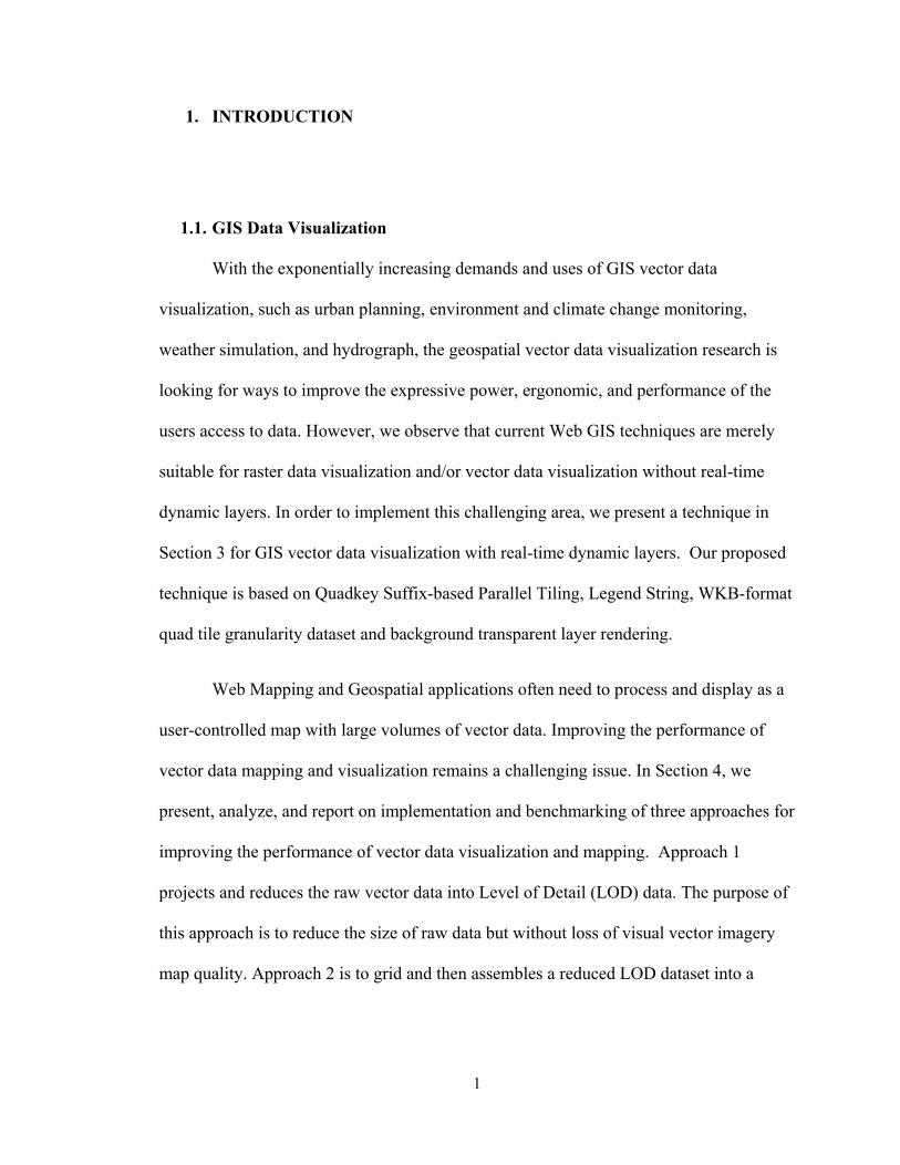
1. INTRODUCTION

1.1. GIS Data Visualization

With the exponentially increasing demands and uses of GIS vector data

visualization, such as urban planning, environment and climate change monitoring,

weather simulation, and hydrograph, the geospatial vector data visualization research is

looking for ways to improve the expressive power, ergonomic, and performance of the

users access to data. However, we observe that current Web GIS techniques are merely

suitable for raster data visualization and/or vector data visualization without real-time

dynamic layers. In order to implement this challenging area, we present a technique in

Section 3 for GIS vector data visualization with real-time dynamic layers. Our proposed

technique is based on Quadkey Suffix-based Parallel Tiling, Legend String, WKB-format

quad tile granularity dataset and background transparent layer rendering.

Web Mapping and Geospatial applications often need to process and display as a

user-controlled map with large volumes of vector data. Improving the performance of

vector data mapping and visualization remains a challenging issue. In Section 4, we

present, analyze, and report on implementation and benchmarking of three approaches for

improving the performance of vector data visualization and mapping. Approach 1

projects and reduces the raw vector data into Level of Detail (LOD) data. The purpose of

this approach is to reduce the size of raw data but without loss of visual vector imagery

map quality. Approach 2 is to grid and then assembles a reduced LOD dataset into a

2

Quadtree granularity dataset, to reduce the dataset granularity in order to speed up the

data retrieval and loading. Approach 3 is server-side vector data caching.

1.2. My Work

The objective of this research is to achieve the challenging and unimplemented

areas in GIS data visualization and its performance improvement.

The Section 3 presents a GIS vector and raster data visualization with real-time

dynamic layers. The ability of real-time dynamic layers is gained by the techniques of our

proposed Quadkey Suffix-based Parallel Tiling, Legend String, WKB-format quad tile

granularity dataset and background transparent layer rendering. Two of implementations

of vector data visualization applied with our proposed techniques are presented.

In order to make vector data visualization as fast and responsive as possible, three

approaches for improving the performance of vector data visualization are formed,

proposed and implemented in Section 4. Approach 1 intends to project and reduce the

raw vector data into LOD data. The purpose of this process is to reduce the size of raw

data but without loss of visual map imagery quality. Approach 2 is proposed for gridding

and assembling reduced LOD dataset into Quadtree granularity dataset, it intends to

reduce the dataset granularity to speed up the data retrieval and loading. Approach 3 is

the server side vector data caching. Approach 1 and 2 are pre-processing that designed

for speeding up the vector data rendering and loading during the first time request. They

reduce the overhead unnecessary and redundant in real time computation. Approach 3 is

used to expedite the response time for the vector data that have been cached in database.

It is designed for the second time and succeeding requests performance improvement.

3

1.3. The Organization of the Dissertation

The organization of this dissertation is structured as follows:

Chapter 2: States the GIS background techniques focus on standard GIS vector

and raster data format, the GIS coordinates system.

Chapter 3: Presents a GIS vector and raster data visualization with real-time

dynamic layers, including Quadkey Suffix-based Parallel Tiling, Legend String, WKB-

format quad tile granularity dataset and background transparent layer rendering, the

algorithm of vector labeling of Point, LineString and Polygon. At the end of this section,

two of implementations of vector data visualization applied with our proposed techniques

are presented.

Chapter 4: Describes a comprehensive performance improvement solution, it

includes three approaches: projects and reduces the raw vector data into Level of Detail

(LOD) data, grid and then assembles a reduced LOD dataset into a Quadtree granularity

dataset and server-side vector data caching. Finally, we perform and describe 14

experimental tests in 6 scenarios and the experimental test results were expected as our

system applied with the comprehensive performance improvement solution.

At each end of section we present a summary of this dissertation in terms of an

overview of the contribution and future directions of this research.

4

2. GIS Background

2.1. Vector Data Format

2.1.1. Shapefile

The Shapefile[1][2][3] is a geospatial vector data format for GIS established by

ESRI[1][2]. The format of our raw vector data is in shapefile format which are the current

industry standard and work with most all GIS commercial software products and other

open source applications. In general, a shapefile is a set of three files that store the vector

data records that comprises a shapefile: ".shp", ".shx", ".dbf". [1][2][3].

Since the shapefile standard formed in 1980s, [3] presents 3 key limitations for

current GIS as follows:

• The maximum size of either “.shp” or “.dbf” component files cannot

exceed 2 GB.

• Maximum length of field names is 10 characters and maximum number of

fields is 255.

• A shapefile cannot store type-mixed vector data

Typically, the shapefile format has less flexibility and scalability to perform any

record (or vector object)-level operations, such as grouping records, records alteration.

5

2.1.2. Well-Known Binary

The WKB representation for geometric values is defined by the OpenGIS

specification. Since shapefile format has several key limitations, the WKB (Well-Known

Binary) [4] vector data format is modeled, employed and applied in our vector

visualization in Section 3.4.2. Compared to shapefile format, the WKB format has three

main advantages over shapefile format described in [4] as follows:

1. No maximum size limitation. No maximum length of field names limitation.

And no maximum number of fields limitation

2. Capable of mixed type of vector data

3. Capable of record (object) granularity operation.

2.2. Raster Data Format

Our geospatial raster raw data are from various sources, such as USGS Digital

Orthophoto Quadrangles (DOQs), County Photography, Ikonos Satellite Imagery and

Geoeye. All raster raw data which from various sources are in TIFF (Tagged Image File

Format [5]) format to store digital satellite images with embedding geographic

information, such as latitude, longitude, map projection etc.

[5] defines a three-level hierarchy: 1. a file Header. The file header contains the

geospatial information such as as latitude, longitude, and map projection etc. 2. One or

more directories called IFDs (Image File Directories), containing codes and their data, or

pointer to the data. 3. Data. The data is the pixels of this imagery.

6

2.3. The Projection System

2.3.1. UTM

All of our raster raw data are in UTM [6] projection. [6] describes the UTM

system divides the surface of Earth between 80°S and 84°N latitude into 60 zones, each 6°

of longitude in width and centered over a meridian of longitude. Zone 1 is bounded by

longitude 180° to 174° W and is centered on the 177th West meridian. Zone numbering

increases in an easterly direction. Each of the 60 longitude zones in the UTM system is

based on a transverse Mercator projection, which is capable of mapping a region of large

north-south extent with a low amount of distortion. [6]

[6] describes UTM projection has following main disadvantages:

1. A full reference requires a zone number and easting and northing coordinates.

2. The axes in adjacent zones are skewed. Therefore, problems arise when

working across zone boundaries.

3. No mathematical relationship between coordinates in one zone and those in an

adjacent zone.

2.3.2. Tile Mercator

Considering the disadvantage of UTM, [7] proposes and introduces the Tile

Mercator Projection System, which solves all projection problems that are happened in

UTM. The Tile Mercator projection system is a close variant of the Mercator projection,

which looks like as follows:

7

Figure 1 Tile Mercator Projection

The Tile Mercator has two important properties that outweigh the scale distortion

described in [7] is following:

1. Conformal Projection: means that it preserves the shape of relatively small

objects.

2. Cylindrical Projection: means that north and south are always straight up and

down, and west and east are always straight left and right.

In addition to the projection, the ground resolution or map scale is specified in

order to render a map in [7]. The ground resolution indicates the distance on the ground

that is represented by a single pixel in the map. For example, at a ground resolution of

100 meters/pixel, each pixel represents a ground distance of 100 meters. The ground

resolution varies depending on the level of detail and the latitude at which it’s measured.

8

[7] also defines that at the lowest level of detail (Level 1), the map is 512 × 512

pixels. At each successive level of detail, the map width and height grow by a factor of 2.

For instance, Level 2 is 1024 × 1024 pixels, Level 3 is 2048 × 2048 pixels, and Level 4 is

4096 × 4096 pixels, and so on.

[7] generalizes the width and height of the map (in pixels) at successive each level

can be calculated as:

256 2levelwidth height= = ×

9

3. The GIS Vector and Raster Data Visualization

In this section, we presents the quadtree-based indexing and tiling techniques,

parallel map tiling infrastructure and its implementation, algorithm of vector Point

labeling, algorithm of LineString segments merging, algorithm of convex and non-

convex Polygon labeling, the PNG [8] and KML [9] output, Legend String, time series, a

comprehensive performance improvement solution, the algorithm of raster data re-

projection and an implementation of server side geospatial data LRU caching algorithm.

3.1. System Architecture

The dynamic vector and raster data visualization parallel map tiling system is a

web service-based GIS system through the internet.

The capability provided to the user is the vector and raster data visualization,

virtual fly over maps comprised of raster satellite imagery overlaid with vector data. This

data visualization is able to assistant users to explore, analysis the vector and raster data.

All of this data visualization capability builds on multi-tiers system architecture, it

includes:

1. Vector data visualization engine and vector datasets and databases

2. Raster data visualization engine and raster datasets and databases

3. JavaScript-based and Flash-based Client side navigation application

4. cluster servers

10

Figure 2 The System Architecture

3.2. Quadtree-based Parallel Tiling

3.2.1. Quadkey

[7] proposes and presents the Tile-based Square Mercator projection, and this

Tile-based Square Mercator projection is applied in our vector data visualization system.

In this projection, the latitude and longitude are on the WGS 84 datum. The longitude is

assumed to range from -180 to +180 degrees, and the latitude is clipped to range from -

85.05112878 to 85.05112878.

Large-scale Raster Datasets Large-scale Raster Datasets and Databases

Raster Data Visualization Engine

Vector Data Visualization Engine

Cluster Side Caching

JavaScript-based Navigation Application

Flash-based Navigation Application

Cluster Servers

11

In terms of this square projection, our rendered map in our system is cut into 256

by 256 pixels each. [7] describes the tile coordinates and quadkey to index each tile as

follows:

• Each tile is given XY coordinates ranging from (0,0) in the upper left to

1 1(2 ,2 )n n− − in the lower right, where n is the number of level. For example,

at level 3 the tile coordinates range from (0,0) to (7,7) . Given a pair of

pixel XY coordinates, tile XY coordinates can be determined by pixel

coordinates as follows:

/ 256x xt p=

/ 256y yt p=

• The two-dimensional tile XY coordinates is able to be combined into one-

dimensional strings in Quaternary called Quadkey by interleaving the bits

of the Y and X coordinates. For instance, given tile XY coordinates of (1,

2) at level 3, the quadkey is deducted as follows:

1 001x Dec Bint = =

2 010y Dec Bint = =

2 001001 021 "021"Dec Bin Quaq = = = =

3.2.2. Quadkey Suffix-based Parallel Tiling

Our map is organized by level of details. At the lowest level of detail (Level 1),

the map is 512 by 512 pixels. At each successive level of detail, the map width and height

12

grow by a factor of 2: Level 2 is 1024 by 1024 pixels, Level 3 is 2048 by 2048 pixels,

and Level 4 is 4096 by 4096 pixels, and so on. It is defined as follows:

1

2

21

512 512

1,024 1,024

536,870,912 536,870,912

l

lL

l

× × = = ×

The corresponding ground resolution (meter) in our system is shown as following:

1

2

21

78,271.5170

39,135.758

0.075

g

gG

g

= =

A quadtree is a tree data structure in which each internal node has exactly four

children. The Quadkey is used to identify each tile in our quadtree organized maps. Since

our rendered map is gridded into 256 by 256 pixels each, in terms of property of quadtree,

we proposed a 4n tiling approach. The purpose of this approach is to make one map tile

mapped for one server. This approach intends to cut a whole map into smaller tiles, and

hence the computation for a whole map, like labeling, data retrieving and loading, are

divided into a smaller computation with tile granularity. These divided computations are

able to be carried out simultaneously by clustered servers. In other words, this approach

allows one tile mapped into one server and thus its corresponding computation is

assigned to this one server. Finally, our client navigation application collects the divided

map tiles and gathers the divided tiles, and then reverts them into a whole map.

13

In theoretical, the performance of 4n tiling system is in direct proportion to the

number of servers. In practical, 34 8 8 64= × = tiles that equal 2048 2048× pixels, this

pixels area could be covering by most popular monitors. To optimize the performance of

map retrieval, display and save energy, 8 8× tiling is applied and implemented in our

system. The one-server-to-one-tile mapping is shown in Figure 3.

Figure 3 Tile Server Mapping

The Quadkeys have some interesting properties. First, the length of a quadkey

equals the level of details in tile. For example, tile 001 is in Level 3. Second, the quadkey

of tile starts with the quadkey of its parent. For example, tile 0010 is a child of tile 001.

Finally, The tiles is able to be grouped by the prefix of quadkey and the suffix of quadkey.

In terms of properties of quadkey, in order to mapping and indexing tiles to severs, we

14

further propose a 8 8 quadtree suffix-based indexing algorithm. The Figure 4 shows 8 8 quadtree suffix-based indexing:

000 001 010 011 100 101 110 111

002 003 012 013 102 103 112 113

020 021 030 031 120 121 130 131

022 023 032 033 122 123 132 133

200 201 210 211 300 301 310 311

202 203 212 213 302 303 312 313

220 221 230 231 320 321 330 331

222 223 232 233 322 323 332 333

Figure 4 8×8 quadtree suffix-based indexing

In Figure 4, for example, tile 001 assigned to server 001 . And any map tile

having the 001 suffix of quadkey, such as 012001, 10231001etc., is expected to be

assigned to the server 001 . In other words, the 001 is able to mapping the tiles in Level

3 and the tiles fall in after Level 3 but having suffix 001 . As for the 20 tiles in Level 1 (4

tiles) and Level 2 (16 tiles), they randomly assigned to any server in an 8 8× cluster.

Furthermore, building less than 8 8× the number of servers is feasible in our approach.

In case of the 24 4 4 16= × = servers (shown in Figure 3), any map tile having the 01

suffix of quadkey, such as 012001, 10231001, etc., is expected to be assigned to the

server 01 .

00 01 10 11

02 03 12 13

20 21 30 31

22 23 32 33

Figure 5 4×4 quadtree suffix-based indexing

15

3.3. The Resource Availability Management

The parallel tiling is eligible to support resource pool-based consumption model

[10]. The VM resource pool has a real-time list with all of available VMs. Once one of

VMs gets failed, the monitoring system would put any available VM to fill this absence.

3.3.1. The Failover Strategy

The right neighbor failover strategy is selected for our Failover Strategy. The

right neighbor is able to be easily determined by Quadkey :

1r cQuadkey Quadkey= +

Where Quadkey is a quaternary number, cQuadkey denotes the Quadkey of

current server, rQuadkey is denoted as the right neighbor of cQuadkey .

Once a server gets failed, the server availability list would be getting updated, and

the system put the right neighbor server to take the computation for tiles which assigned

for that failed server. And the system notifies this failure to administrator.

After failed server fixed up, the system recovers the status before this failure and

updates the availability server list.

16

3.3.2. The Feedback Loop-based Monitoring

Feedback loops based system takes the system real-time status into consideration.

The system monitor takes the initial resource allocation first, and then it monitors every

working VM.

Every 5 seconds, the resource availability management system monitor scans

entire VMs. Once a VM failure is found, it updates the VM availability list. The VM

availability list shared with the client navigation application, it requests to VMs on this

updated list then. This feedback loops based process provides availability guarantees.

Figure 6 The Resource Availability Management

17

3.4. GIS Vector Data Visualization with Real-Time Dynamic Layers

With the exponentially increasing demands and uses of GIS vector data

visualization, such as urban planning, environment and climate change monitoring,

weather simulation, and hydrograph, the geospatial vector data visualization research is

looking for ways to improve the expressive power, ergonomic, and performance of the

users access to data. However, we observe that current Web GIS techniques are merely

suitable for raster data visualization and/or vector data visualization without real-time

dynamic layers. This paper presents a technique for GIS vector data visualization with

real-time dynamic layers. Our proposed technique is based on Quadkey Suffix-based

Parallel Tiling, Legend String, WKB-format quad tile granularity dataset and background

transparent layer rendering.

3.4.1. Introduction and Related Work

GIS data represents the real world’s geographic objects (such as streets, lakes,

lands, cities etc.) in digital world. Traditionally, there are two broad types used to store

data in a GIS: raster data and vector data [11][12][13]. A raster data type (digital image)

is essentially represented by graphical cell grid (typically, it is a pixel). Typically, vector

data is composed of discrete coordinates that can be used as Point or connected to create

LineString and Polygon.

[14] describes there are two principal methods to visualize vector data. (1) A set

of vector data is rasterized at a given resolution as an image and combined with other

images (e.g., road system combined with topographic map) (2) Vector data is mapped by

primitives such as points, lines, and polygons, which can be modified by point symbols,

18

line patterns, or polygon styles. The first strategy is to rasterizing vector data as images in

a pre-processing step. The image is used as texture and projected onto the level-of-detail

terrain geometry. Using multi-overlaying, different rasterized vector data sets can be

visually combined [15]. However, the rasterized images require additional storage space,

and the orders of layers and level cannot be changed without rasterizing the vector data

again [14]. Our work falls primarily into the second category. Our vector data

visualization is the use of geography WKB-format primitives Point, LineString and

Polygon, composed of geography coordinates, to represent map images in real-time. In

this strategy, the ability of real-time dynamic layers is feasible since the orders of layers

and level is able to be changed during real-time.

In recent years, various open source applications to vector data visualization GIS

have been developed and published. In general, [16] represent vector data fall in the first

strategy. The ability of dynamic layers is not allowed in [16]. [17] and [18] represent

vector data in the second strategy. In the field of vector data visualization, [17] visualizes

vector data based on XML, which defines a wide variety of vector objects and styles.

And [17] mainly focuses on LineString (street) object. [18] visualizes vector data based

on shapefile, which is not able to handle large volume data (greater than 2GB). None of

them allow the ability of real-time dynamic layers.

In general, the strategy and algorithm with vector data visualization have not

changed much in principle for years. However, recently, approaches towards vector data

transmission have been emerged and applied, for example, to progressively transmit

[19][20] [21]and/or compress [22] vector data. They do not concentrate on the

19

visualization of vector data, but can substantially support the design and implementation

of visual multi-resolution representations of vector data.

3.4.2. GIS Vector Data Modeling

WKT and WKB [4] (A binary equivalent with WKT) are selected and

implemented as our vector data representations. The data in WKT and WKB are

organized by records, each of which represents an object in a GIS vector data layer. The

GIS vector WKT and WKB formats are regulated by the Open Geospatial Consortium

(OGC) [4] and described in their Simple Feature Access and Coordinate Transformation

Service specifications [4]. In terms of OGC specification, we define a geospatial vector

set S composed by vector V

as following:

The geospatial vector set

1

n

i

V

VS

=

Where n is natural number greater than 1

Since the attributes are metadata attached to a geospatial object, we simple define

a geospatial vector V

with its vertices v as following:

V

= 1 2[ , ,..., ,...,

[

]

]

i mv v v v

v

Where each v or iv is formed by the coordinate (latitude, longitude) and m is natural

number greater than 1

V

is a vector of vertices

Each iV

is a vector of attributes

v is a vertex of the Point vector

Each iv is a vertex of the LineString or

Polygon vector

20

The Point vector

PTV

= [ ]1v

Due to any vertex can be presented by a pair with geography coordinates

( , )latitude longitude , PTV

is denoted by a coordinates representation is as following:

PTV

= 1 1( , )latitude longitude

These coordinate numbers are often arranged into a row vector or column vector,

particularly when dealing with matrices. And the (lat, long) is used to indicate

( , )latitude longitude as following:

1 1 [ , ]PTV lat long=

LineString vector

LSV

= [ ]1 2,..., ,...,, i mv v v v

Where each iv is formed by the coordinate (latitude, longitude) and m is natural

number greater than 1

Polygon vector

PGV

= [ ]1 2 1,..., ,..., ,, i mv v v v v

Where each iv is formed by the coordinate (latitude, longitude) and m is natural

number greater than 1

In general, any type of vector can be defined as follows:

21

[ ][ ]

[ ]

1

1 2

1 2 1

,..., ,...,

,..., ,..., ,

,

,i m

i m

v

V v v v v

v v v v v

=

Where each iv is formed by the coordinate (latitude, longitude) and m is

natural number greater than 1

3.4.3. Vector Data Labeling

The vector data visualization is drawn with 3 different types of objects:

• Points, representing top of mountains, cities, airports, etc.

• Lines, representing rivers, streets, etc.

• Polygons, representing countries, states, provinces, lakes, parcels, etc.

In the case of labeling a vector object, the text is placed around the object. The

goal of point labeling is to find a position for each label in such a way that no label

overlaps another one or overlaps the symbol marking a point. [23]

The Circle Detecting Algorithm

A proposed Circle Detecting Algorithm is to avoid conflict and limits labels to four candidate positions around a labeling position, which are listed as following:

o0θ =

o90θ =

o180θ =

o360θ =

22

All labels are ASCII-based characters, each of them on map occupies a circle

position fully fits itself is proposed, shown in below:

Figure 7 The Circles around Letters

The circle detecting is that each circle of character of label cannot overlap with

the others circle of characters of labels, in this proposed algorithm, it has two functions,

one is IsSelfTwoCircleOverlaped and IsTwoCircleOverlaped.

The purpose of function IsSelfTwoCircleOverlaped is to check if two characters

in same label are overlapped, the main idea is to check if the distance of two same size

circles is greater than the sum of two circles’ radiuses.

The function IsTwoCircleOverlaped is intend to check if two characters from

different labels are overlapped, the principle idea is as same as the function

IsSelfTwoCircleOverlaped, but it has three cases, one is for the big font labels checking,

the other is for some special point labeling such as very density points labeling, the last

one is for the regular overlap checking. The different of them is only the distance of two

circles, the big font labels overlay checking has the smallest distance capability, and the

special point labeling has the biggest distance capability.

Since a map is drawn with 3 different types of elements: Point, LineString and

Polygon, obviously, each of them has different labeling approaches:

23

1. The Point labeling always be labeled horizontally.

2. The LineString labeling has much different way to be drawn since it is not

always be horizontal but its labeling almost always oriented in a direction

locally parallel to the line.

3. The Polygon labeling always be labeled horizontally but the Polygon object

positing is much more complicated.

The Point Horizontal Labeling

On a map, a character of one label of a point object can be included in a circle of

radius r. The label of this object cannot overlap with this circle. The candidate positions

for a point object are spread as regularly as possible around this circle. Point object are

almost always labeled horizontally in practice. Our Point label placing rule is followed

our regular placing rule which allows four positions to be labeled, it listed in Figure 16.

Figure 8 The World_Nations Layer Horizontally Labeled

Figure 18 shows the Point vector data (World_Nations Layer) horizontally labeled

on our vector map engine.

24

The LineString labeling

The LineString labeling has following 2 steps:

1. Merging the segment objects into one LineString object

2. Labeling the LineString object with oriented in a direction locally parallel to

the line, as well as each character in one label is to perpendicularity to the line.

1. Merging the Segments into LineString

The LineString objects (roads, streets, highways) are represented with broken line

objects (the segment object) in original vector data format (shapefile).

Therefore, there would be many duplicated segment labels to be drawn on the

map if the LineString objects to be labeled directly from original shapefile without any

object merging. Given figure 19 is to show this duplicated segment labeling:

Figure 9 Many Duplicated Segments Labeling

25

To avoid this, first of all, in each map tile (256pixles*256pixles), merging as

many segments (which belongs to the one same LineString object) as possible into one

LineString object is needed. Figure A2 and A3 show this merging process:

First, checking if two segments have the same LineString object name, if so,

second, checking if the starting point and ending point of two segment have the same

coordinates, if so, merging them into one LineString object, all of the others cases, ignore

them , which means all of them are in different LineString object.

Figure 10 Merged LineString Labeling

Figure 10 shows the LineString labeling in our vector map engine after applied

merging algorithm, the result is not crowd and easy to read.

2. Labeling

In practice, the label associated with a line is almost always oriented in a direction

locally parallel to the line, as well as each character in one label is to perpendicularity to

the line.

26

Our LineString label placing rule limits LineString labels to three possible

candidate positions along with a line, which includes the middle position, the one-third

position (at one-third away from the starting point), and the two-third position (at two-

third away from the starting point). Once any character in any label cannot be placed, it

would be trying to the next candidate position until placed or ignored (which means there

is no space to be placed).

Figure 11 illustrate how candidate positions are generated for LineString.

Figure 11 Three Candidate Labeling Position

The Polygon Labeling

The Polygon object labeling has much more complicity than Point and LineString

labeling, since Polygon labeling has much more cases need to be considered:

1. The very small polygon labeling

2. The very big polygon labeling

3. The regular polygon labeling

To define if a polygon is a very small polygon or not, the spatial bounding box

(The minimum bounding rectangle) is needed. The minimum bounding rectangle (MBR),

also known as bounding box or envelope, is an expression of the maximum extents of a

27

2-dimensional object (e.g. point, line, and polygon) within its 2-D (x, y) coordinate

system, in other words min(x), max(x), min(y), max(y). [24]

1. The very small polygon labeling

A very small polygon can be considered as a point object. In our system, the very

small polygon is defined as a polygon whose spatial bounding boxes (The minimum

bounding rectangle) occupies the area less than 20 40 pixels× in each corresponding

resolution. The candidate generation is done as for point object in this case.

2. The very big polygon labeling

Basically, the very big polygon labeling, like continental, country, province or

states, would be shown only at very zoom-out resolution, the very big polygon labeling

always be labeled horizontally in the center of Polygon object.

3. The regular polygon labeling

The regular polygon labeling should always be labeled horizontally in the center

of Polygon object.

3.4.4. Legend String

Legend String (LS) is a layer control convention between the user interfaces

(client application) and the backend vector data visualization system. The client

application collects user commands by a flash-based checklist toolkit Legend Layer

Control. The Legend Layer Control lists all available layers in it and provides checkboxes

to allow the user to customize the layer composition. Once the layers are checked, the

28

client application collects user’s commands and converts the commands into LS and

finally sends the customized LS to the backend vector data visualization system. The

convention of Legend String has three syntaxes to customize map layers:

1. Layers Priority: The + is used to delimit layers in LS. The order of layers in

LS reflects the priority of layer rendering. For instance, layerA layerB+ means that both

layerA and layerB rendered in map, and layerA has higher rendering priority of than

layerB .

2. Level Visibility: The – is used to indicate the level range of layer visibility.

Given a lower bound level and an upper bound level with delimited by a symbol – , the

layer is expected to be shown within this specified level visible range.

3. Layer Coloring and Transparency: The color and transparency values in LS

are typically expressed using 8 hexadecimal digits, with each pair of the hexadecimal

digits representing the sample values of the Alpha, Red, Green and Blue channel,

respectively. For example, the Legend String 80FFFF00 represents a 50.2% opaque

yellow.

While the 21-level views setup in our system, for every vector dataset, we pre-

generate 21 vector subsets for each level of detail. Since the difference of pixel spaces in

each level of details, at some cases, especially in zoomed-out levels, some vertices in

vector object that are all going to render into the same pixel on screen. In terms of this

principle, a pixel distance based data reduce process is applied in the 21 vector subsets.

Because our map is cut into a 256 256× pixels tile each, and its relatively low

29

granularity provided by the tile causes many vertices or objects in 21 vector subsets not

in the tile-of-view to be loaded, we propose a tile granularity subset that only containing

the vertices and objects to be rendered in the tile-of-view. The tile granularity subset is

determined by a quad tile intersecting with its corresponding 21 level subsets. For

example, tile 0 subset at level 1, it is determined by an square area of [(0,0), (256,0),

(256,256), (0, 256), (0,0)] intersecting with level 1 subset. We define a ST_intersect

geography process followed OpenGIS Specifications (Standards) [4] as follows:

_ ( ; )liij ijT ST Intersect s t=

A semi-colon delimits two arguments liijan tds , ljs denotes LOD subset at level i,

ijt is used to indicate the jth tile at level i, ijT denotes the jth tile subset at level i, n is the

number of level, the subsets at level i is denoted as follows:

[ ]1 2, ,...,iTi i ims T T T=

:where

4nm =

The entire 21-level subsets gridded into Tile subsets are denoted by TS as follows:

1 2 21, ,...,T T TTS s s s =

30

3.4.5. Quad Tile Dataset Representation

WKB

The GIS vector WKB format are regulated by the Open Geospatial Consortium

(OGC) and described in their Simple Feature Access and Coordinate Transformation

Service specifications [4]. In system, WKB are selected and implemented as our vector

data representations. The data WKB are organized by records, each of which represents

an object in a vector data layer. In terms of WKB specification, our Point PTV

,

LineString LSV

and Polygon PGV

vector data in LOD pixel coordinates which converted

from latitude and longitude that on the WGS 84 datum are defined as follows:

PTV

= ,x yP P

LSV

= [ ]1 2, ,..., ,...,i mv v v v ,1m i m∈ ≤ ≤N

:where

iv = ,xi yiP P

PGV

= [ ]1 2 1, ,..., ,..., ,i mv v v v v ,1m i m∈ ≤ ≤N

:where

iv = ,xi yiP P

, x yP P denote the pixel coordinates in two-dimension XY.

31

Quad Tile Dataset

While the 21-level views setup in our system, for every vector dataset, we pre-

generated 21 vector subsets for each level of detail. Since the difference of pixel spaces in

each level of details, at some cases, especially in zoomed-out levels, some vertices in

vector object that are all going to render into the same pixel on screen. In terms of this

principle, a pixel distance based data reduce process is applied in the 21 vector subsets.

Because our map is cut into a 256 256× pixels tile each, and its relatively low

granularity provided by the tile causes many vertices or objects in 21 vector subsets not

in the tile-of-view to be loaded, we propose a tile granularity subset that only containing

the vertices and objects to be rendered in the tile-of-view. The tile granularity subset is

determined by a quad tile intersecting with its corresponding 21 level subsets. For

example, tile 0 subset at level 1, it is determined by an square area of [(0,0), (256,0),

(256,256), (0, 256), (0,0)] intersecting with level 1 subset. We define a ST_intersect

geographic process followed the OpenGIS Specifications (Standards) as follows:

_ ( ; )iij ijT ST Intersect s t=

A semi-colon delimits two arguments iijs , t , is denotes LOD subset at level i, t

is used to indicate the jth tile at level i, ijT denotes the jth tile subset at level i, and hence,

the subsets at level i is denoted as follows, where the indicates the number of tile at

level i:

32

[ ]1 2, ,...,ii i ims T T T=

:where

4nm =

The entire 21-level subsets gridded into Tile subsets are denoted by as follows:

1 2 21, ,...,S s s s =

3.4.6. Real-Time Dynamic Layers

The advantage of our vector data visualization system is its real-time dynamic

layer. The ability of the real-time dynamic layers is to allow any vector layer overlaying

any other vector layers in any order during real-time (at least the average response time

less than 1 seconds, to meet our “real-time” criteria). The ability of real-time dynamic

layer is gained by the techniques of Legend String, WKB-format quad tile granularity

dataset and background transparent layer rendering.

The Legend String and WKB-format tile dataset are presented in Section 2 and 3,

respectively. The ability of background transparent layer rendering is gained by alpha

channel technique in Portable Network Graphics (PNG). 32-bit PNG and added an alpha

channel (8 bits) to control the level of transparency is implemented in our vector data

visualization system. The alpha channel basically controls the transparency of all the

other channels. By adding the alpha channel to a map tile image, our system is able to

control the transparency of the red channel, green channel and the blue channel [25][26].

Shown in Figure 4, we build a base layer with fully opaque and set the background of

each layer to be fully transparent to seamlessly make any vector layer overlaying with

others vector layers.

33

3.5. Raster Data Visualization

3.5.1. Raster Data

Raster data are cell-based spatial datasets. There are also three types of raster

datasets: thematic data, spectral data and pixel-based pictures. The pixel-based pictures

format is the only source of our raster imagery engine. Unlike vector data, raster imagery

data is formed by each pixel.

3.5.2. Re-projection

Most of our raw raster data are in UTM projection. Considering the disadvantages

of UTM projection system, the Tile Mercator projection is applied to our raster imagery

engine. Therefore, an UTM to Tile Mercator re-projection is pre-processed in our raster

engine, which has two major steps:

• A re-projection from the UTM to the Tile Mercator

Base Layer

Dynamic Layers

Figure 12 Dynamic Map Layers

34

• A conversion from a large tiff image to the quadtree-based JPEG image

tiles.

The Related Work

[27][28] concludes two major re-projection methods have been widely used in

image process as follows:

1. Area Weighted Convolution (AWC) [29], which assumes square pixel of

uniform activity,

2. Gaussian-pixel convolution (GPC) method, it assumes the activity of each

pixel is represented by a Gaussian function.[30][31]

The Re-projection from UTM to Tile Mercator

The UTM to Tile Mercator re-projection algorithm is an AWC-based, pixel-

driven, nearest-neighbor algorithm. Each nearest-neighbor’s weigh is treated as the same

weight during the re-projection process. The nearest-neighbor is a neighbor pixel next to

targeted pixel.

Figure 13 shows Pixel 1, 2, 3, 4, 6, 7, 8 and 9 are the nearest-neighbors of targeted

pixel 5.

Pixel 1 Pixel 2 Pixel 3 Pixel 4 Targeted Pixel 5 Pixel 6 Pixel 7 Pixel 8 Pixel 9

Figure 13 Targeted Pixel and its Nearest-neighbors in Matrix Pixels

35

The re-projection from UTM to Tile Mercator has two steps:

• The images in UTM: Loop all of the pixels, for each pixel, calculating the

average color value from this pixel and its all of nearest-neighbors. All pixels

are treated as the same weight.

• The image in Tile Mercator: converting each UTM Pixel Coordinates to Tile

Pixel Coordinates. In Tile image, addressing this pixel and setting the color

value of this Tile Mercator image pixel as the average color value from its

corresponding UTM image pixel and UTM image pixel’s all nearest-

neighbors.

Gridding the UTM Images to the Tile Mercator Images

Our raster raw data are from various sources, such as USGS Digital Orthophoto

Quadrangles (DOQs), County Photography, Ikonos Satellite Imagery and Geoeye, all

various sources raster raw data are in TIFF with UTM to store digital pixels and with

embedding geographic information.

The TIFF is a bitmap imagery format, and JEPG is a lightweight image format

with much smaller size. Considering the data shipping, to archive the best performance,

the JEPG is used as our raster data format.

In terms of Quadtree indexing system, all raster images are organized by Quadtree

data structure. Therefore, each raster imagery tile is a JPEP image with 256 by 256 pixels

in Tile Mercator.

36

These gridded raster imagery tiles finally are formed in a Quadtree-based dataset.

And each source has one Quadtree-based dataset. And each tile has a unique key as

follows:

A unique key = source name + quadkey.

The UTM to Tile Mercator image gridding algorithm has following steps:

• The Bottom Level Gridding

Current bottom level is the Level 21 (resolution=0.075 meter). In this level,

cutting source images into 256 pixels by 256 pixels each, each tile assigned a unique key

after its generated.

• The Rest of Levels Processed in Bottom-up Gridding

After Level 21 tiles generated, Level 20 is the next. In terms of the Level of Detail,

a square area of one Level 20 tile covered equals four Level 21 tiles covered. Therefore, a

bottom-up processing is formed as follows:

1. For each tile in Level 20, merging its four children tiles from Level 21 into

one tile with 4×256×256 pixels

2. Cutting this tile into 256×256 grids, each grid has 4×4 pixels, calculating the

average color value from this grid.

3. For each pixel of Level 20, setting its value as the average color value from

the grid

37

After Level 20 is ready, Level 19 is the next. This process is repeated until the top

level, Level 1. This generation process designed from the bottom of the system to the top

of the system, it is a bottom-up gridding.

A Re-projection from UTM to Tile Mercator

UTM to Tile Mercator re-projection is a pre-processing as follows:

• Re-projecting UTM images into Tile Mercator images.

• Converting the raw tiff large images into the quadtree-based JPEG tiles.

The UTM to Tile Mercator re-projection algorithm is applied in Step 1, the UTM

to Tile Mercator image gridding algorithm implemented in Step 2. This pre-processing is

formed in following detailed steps:

o Parsing the TIFF to retrieve geospatial information and saving this location

information to plaint file

o Getting the tile’s 4 vertices coordinates and its resolution from plaint file

o Creating a hash table to save tiles’ unique quardkey and its geospatial

information.

o Cutting the bottom Level 21 tiles:

When process a TIFF image:

o Verify this quadkey is hit existed in hash table,

38

o Hit: generating the quadkey and cutting TIFF into the JEPG tile image,

inserting this quadkey and information into the hash table

o No Hit: loading this tile and form steps as follows:

For each pixel when (pixel.RGB == 000000)

Filling the color value of this pixel as the average color value from its

corresponding UTM image pixel and UTM image pixel’s all of nearest-neighbors.

Bottom-up generating Level 20 to Level 1 tiles:

o For each tile in up level, merging its four children tiles from its bottom level

into one tile with 4×256×256 pixels

o Cutting this tile into 256×256 grids, each grid has 4×4 pixels, calculating the

average color value from this grid.

o For each pixel of up level, setting its value as the average color value from the

grid

The Raster Data Visualization

Shown in Figure 12, the raster data is able to be visualized by building a base

layer as raster imagery and set the background of other vector layers to be fully

transparent. This hybrid mode seamlessly makes the vector data overlaying with raster

data. The hybrid vector and raster data visualization means offering a combined satellite

and map view.

39

3.6. Experiment: Implementations of Real-Time Dynamic Layers

In this section, we present two implementations of our proposed real-time

dynamic layers.

3.6.1. Cluster Setup

All the implementations in this section were conducted on a cluster of 16 virtual

machines provided by TerraFly [32] team. The cluster setup followed our proposed

approach of Quadkey Suffix-based Parallel Tiling, which we described in section 3.3.

3.6.2. Real-Time Dynamic Layers with ADC WorldMap vector data

ADC WorldMap [33] vector data is a topographical background map data of all

countries from the entire world. The data has the most detailed digital atlas at a

1:1,000,000 map accuracy scale. The data are available in the following volumes:

Table 1 ADC WorldMap Vector Volumes

Vector Layer Definition World_Nations Borders for the countries of the World World_Admin Level 1 political boundaries for the countries of the World Airports Airport points and labels BuiltUp_Areas Urban Sprawl Capitals Country Capitals Cities_Greater_900K Cities with population greater than 900,000 Cities_75K_to_900K Cities with population between 75,000 and 900,000 Cities_up_to_75k Cities with population up to 75,000 Cities_Unknownpop Cities with population unknown. World_Cities All cities in the world Cultural_Landmarks Cultural landmarks of the world Water_Poly Lakes and other water polygon features Water_Line Rivers and other water line features Glacier Glacier & other permanent ice fields Seas_Bays Seas and bays labels

40

Grid1 1 degree Lat/Long Grid Grid5 5 degree Lat/Long Grid Grid15 15 degree Lat/Long Grid Mountains Mountain labels Physiography Craters, cliffs, faults, rock outcrops Marine Ports Major marine ports of the world Railroad_Track Railway track Railway_Stations Freight and passenger railway station Major_Routes Major highways and interstates Minor Routes Highways and other routes Utilities Power transmission lines

Two vector data pre-processing are carried out: one is for the reduced 21-level

intermediate subsets for each layer, the other one is for the Quad Tile subsets. Two of

dynamic layers samples loaded with ADC vector data is given as follows:

Sample A :

A sample of a vector visualization map with real-time dynamic layers is shown in

Figure 2:

Figure 14 Sample A Dynamic Layers

41

A Legend String for Figure 5 is composed as follows:

_ _ _ _ _

_

World Nations Water Poly Water Line Major Routes Minor Routes Capitals

World Cities

+ + + + + +

This Legend String denotes that the data visualization composed with layers:

World _ Nations, Water _ Poly, Water _ Line, Major _ Routes, Minor _ Routes,

Capitals and World_Cities. And the rendering priority in this map belongs to:

_World Nations > _Water Poly > _Water Line > _Major Routes >

_Minor Routes > _Capitals World Cities> .

Sample B :

In sample B, we place Utilities and Railrod_Track over the other layers except

base layer World _ Nations . And hence the Legend String and the rendering priority are

modified as follows:

_ _ _ _

_ _ _

World Nations Utilities Railrod Track Water Poly Water Line

Major Routes Minor Routes Capitals World Cities

+ + + + ++ + +

_ _ _ _

_ _ _

World Nations Utilities Railrod Track Water Poly Water Line

Major Routes Minor Routes Capitals World Cities

> > > > >> > >

The layers Utilities and Railrod _ Track on vector map dynamically overlaying

with others is shown in Figure 6.

42

Figure 15 Sample B Dynamic Layers

3.6.3. Time Series with SOAR vector data

A time series is a sequence of dynamic vector layer at real-time, measured

typically at successive times spaced at uniform time intervals (3 seconds). The time series

of vector visualization creates the animated time sequence by fading-in and fading–out

with vector layers in the specific timeline. SOAR stands for the Service Oriented

Atmospheric Radiances [34][35][36]. SOAR vector data provides vector data for AIRS

and MODIS-Aqua, respectively. The SOAR vector data is in a binary format and

logically built with 360 360 grids. Each grid is of 4 bytes that contains the radiance or

brightness value of that particular 1 0.5 gridded region. For instance, the value of the

top left grid denotes the radiance or brightness value of the region of -180 to -179 in

longitude and 90 to 89.5 in latitude. We first convert SOAR format into our WKB format

and we load AIRS and MODIS-Aqua in Channel 20 in following dates:

Table 2 SOAR Vector Volumes

AIRS 01/2005, 02/2005, 04/2005, 05/2005, 07/2005, 08/2005 01/2006, 02/2006, 03/2006, 05/2006, 06/2006, 08/2006 01/2007, 02/2007, 03/2007, 04/2007, 05/2007, 06/2007, 07/2007, 09/2007, 10/2007

43

MODIS-Aqua

01/2005, 02/2005, 03/2005

The two of data pre-processing (21-level subsets and Quad Tile subsets) are

carried out for AIRS and MODIS-Aqua, respectively. Figure 15 shows a Time Series for

AIRS, a Legend String composed with all the loaded AIRS data. Each of AIRS data

divided by Date is set as base layer in each sequence. The layer World_Nationshas less

priority than AIRS and rendered on top of base layer.

Figure 16 AIRS Channel 20 Radiance at 01/2005

Figure 16 shows a MODIS-Aqua Time Series, a Legend String composed with

01/2005, 02/2005 and 03/2005 vector data and the layer World_Nations put on top of

layer MODIS-Aqua.

44

Figure 17 MODIS-Aqua Channel 20 Radiance at 01/2005

3.7. Conclusion and Future Work

In this section, a vector data visualization GIS with real-time dynamic layers is

formed, proposed and implemented. The ability of real-time dynamic layers is gained by

the techniques of our proposed Quadkey Suffix-based Parallel Tiling, Legend String,

WKB-format quad tile granularity dataset and background transparent layer rendering.

Two of implementations of vector data visualization applied with our proposed

techniques are presented. The research for vector data transmission has become

prevalent. In the future, we plan to support the visual multi-resolution representations of

vector data with real-time dynamic layers in our system.

45

4. Performance Improvement of Vector Data Mapping

Web Mapping and Geospatial applications often need to process and display as a

user-controlled map with large volumes of vector data. Improving the performance of

vector data mapping and visualization remains a challenging issue. This paper presents,

analyzes, and reports on implementation and benchmarking of three approaches for

improving the performance of vector data visualization and mapping. Approach 1

projects and reduces the raw vector data into Level of Detail (LOD) data. The purpose of

this approach is to reduce the size of raw data but without loss of visual vector imagery

map quality. Approach 2 is to grid and assemble a reduced LOD dataset into a Quadtree

granularity dataset, to reduce the dataset granularity in order to speed up the data retrieval

and loading. Approach 3 is server-side vector data caching.

4.1. Introduction and Related Work

With the increasing use of the GIS data visualization, the performance of vector

data visualization become of critical concern. In recent decades, LOD and Quadtree [37]

techniques are used widely to facilitate the performance improvement.

LOD techniques provide different representations of the same geometric object,

with each representation having a different level of details. LOD techniques are the

methods used to generate the multiple resolution representations of vector data objects.

Two types of LOD techniques presently used are discrete and continuous LODs. The

discrete multi-resolution representation of polygonal models was proposed in [38].

46

Continuous LODs intend to increase or decrease the resolution of a polygon mesh

through a series of geometry vertices and edges [39]. Continuous LODs was introduced

and implemented in GIS in [7]. Our data reduce work targeted with the second category

Continuous LOD datasets. By using pixel distance in Continuous LOD, we reduce the

raw vector datasets into a hierarchical vector datasets of different levels of detail.

A quadtree is a tree data structure in which each internal node has exactly four

children. The Quadtree data structure has been named and formed in [40] by Raphael

Finkel and J.L. Bentley in 1974. [41] introduces Quadtree into image processing,

computer graphics, geographic information systems and robotic. In recent decades,

Quadtree was widely used in GIS field. [42] describes a quadtree spatial indexing

implemented in a large GIS database product. [43] presents a triangulation model is based

on the restricted quadtree triangulation in a 2D large scale terrain visualization.

Several performance improvements formed in recent decades. [44] presented a

use of pyramids and hash indices on the server side to speed up large maps. Caching is

designed to enhance concurrent data access. Compressed binary representation is

implemented on both server and client sides to reduce transmission volume [45]. There

was no vector data reduce process in [45], the solution in [45] is not able to do neither

vector data culling or handle the vector objects with large amount vertices. [46] presents

a quadtree based data grouping with raw data in order to do polygon culling and solve the

polygon vector objects with large amount vertices. [46] also proposes a vector data

reduce without loss of visual terrain image quality based on level of details, it

dynamically determine the pixel distance and choose the appropriate polygon resolution.

47

[37] focused on polygon vector object only and its dynamic determination solution suit

for a map with different resolution (with elevation data). Our work intends to reduce the

size of raw vector data for all of types: Point, LineString and Polygon. And also a

weighting factor is considered. While many points could be reduced to one point, giving

each point a weighting factor is able to determine which one is expected to be shown on

map. Our data gridding process is based on pre-generated LOD datasets, dealing with

reduced LOD datasets directly. Our data gridding process also is a process for vector data

culling.

In order to make vector data visualization as fast and responsive as possible, three

approaches for improving the performance of vector data visualization are formed,

proposed and implemented in this paper. Approach 1 intends to project and reduce the

raw vector data into LOD data. The purpose of this process is to reduce the size of raw

data but without loss of visual map imagery quality. Approach 2 is proposed for gridding

and assembling reduced LOD dataset into Quadtree granularity dataset, it intends to

reduce the dataset granularity to speed up the data retrieval and loading. Approach 3 is

the server side vector data caching. Approach 1 and 2 are pre-processing that designed

for speeding up the vector data rendering and loading during the first time request. They

reduce the overhead unnecessary and redundant in real time computation. Approach 3 is

used to expedite the response time for the vector data that have been cached in database.

It is designed for the second time and succeeding requests performance improvement.

48

The structure of this part is as follows. Section 1 details the previous relevant

work in this area. Section 2 details a performance improvement solution. Section 3 details

the 14 experiments and their analysis. Section 4 details the conclusion and future works.

4.2. A Performance Improvement Solution

LOD, Level of Detail, our vector map engine have 21 LOD datasets, it is

organized by Levels and its format is WKB.

Actually, LOD datasets is an intermediate datasets for vector map engine, all of

LOD datasets would be processed into Quadtree Nodes Datasets (see Quadtree-based

gridding data), which is the only data source of vector map engine.

LOD datasets generation is a pre-processing for raw data’s reducing, which means

reducing many duplicated vertices from raw data. The duplicated vertices occupy the

same pixel in 256*256 map tile based on Pixel Coordinates.

The purpose of Elimination of Superfluous LOD pro-processing is to ensure one

pixel in final map imagery tile uniquely only represents one geographic vertex of 21-

Level LOD datasets. In other words, thus in view of map tile imagery, using Pixel

Coordinates, the LOD data pre-processing is a lossless data compression process for

shapefile raw data.

49

4.2.1. Vector Data Projection

In order to make the vector data visualization on map seamless and to ensure that

map tiles from different sources line up properly, a single projection for the entire world

is needed. A Tile-based square Mercator projection is applied in our vector data

visualization on map. Since the Mercator projection goes to infinity at the poles, it

doesn’t actually show the entire world. Using a square aspect ratio for the map, the

maximum latitude shown is approximately 85.05 degrees. To simplify the calculations,

we use the spherical form of this projection, not the ellipsoidal form. Since the projection

is used only for map display, and not for displaying numeric coordinates, we do not need

the extra precision of an ellipsoidal projection. The spherical projection causes

approximately 0.33% scale distortion in the Y direction, which is not visually noticeable

[5]. In addition to the projection, the ground resolution or map scale must be specified in

order to render a map, at each successive Level of Detail (LOD), the map width and

height grow by a factor of 2, according our imagery data source, we choose to divide

Level of Detail into 21 levels, the range of ground resolution (meters/pixel) from

78,271.5170 to 0.0746.

4.2.2. LOD

LOD, level of detail, it is defined in Table 1. At the lowest level of detail (Level

1), the map is 512 by 512 pixels. At each successive level of detail, the map width and

height grow by a factor of 2: Level 2 is 1024 by 1024 pixels, Level 3 is 2048 by 2048

pixels, and Level 4 is 4096 by 4096 pixels, and so on. Table 1 shows the LOD levels and

their corresponding map size and ground resolution in our system.

50

Table 3 LOD levels, Map Size and Ground Resolution

Level of Detail Map Width and Height (pixels)

Ground Resolution (meters / pixel)

1 512 78,271.517 2 1,024 39,135.758 3 2,048 19,567.879 4 4,096 9,783.939 5 8,192 4,891.969 6 16,384 2,445.984 7 32,768 1,222.992 8 65,536 611.496 9 131,072 305.748 10 262,144 152.874 11 524,288 76.8 12 1,048,576 38.4 13 2,097,152 19.2 14 4,194,304 9.6 15 8,388,608 4.8 16 16,777,216 2.4 17 33,554,432 1.2 18 67,108,864 0.6 19 134,217,728 0.3 20 268,435,456 0.15 21 536,870,912 0.075

In general, the width W and height H of the LOD map (in pixels) can be

calculated by the width w and height h of a map tile as following:

W H= = 2 iNw × 2 iNh= × 256 2 iN= ×

:where

w h= = 256 pixels

Let M denotes a map set with all of levels maps and m denotes the ith W H×

pixels LOD map.

51

M =

1

2

N

m

m

m

:where

im = i iW H pixels×

Let l

denote a square polygon vector to represent the LOD map with pixel

coordinates, l₁ is a square polygon vector for level 1 map is shown in Figure 1.

Figure 18 LOD Level 1

A square polygon LOD map vector sets L with entire levels l

is denoted as

following:

L

1 1 1 1 1

2 2 2 2 2

, , , ,

, , , ,

, , , ,N N N N N

A B C D A

A B C D A

A B C D A

=

N

l

l

l

=

₁₂

0 1

2 3

,

,

,

: ,

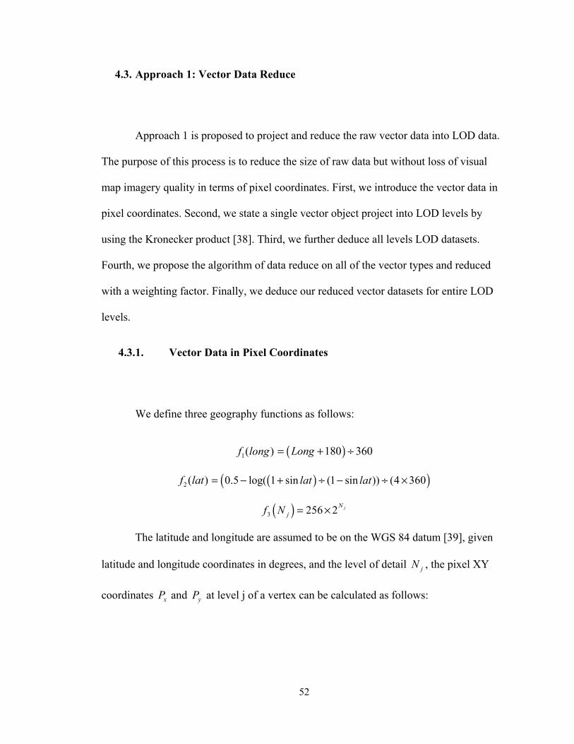
52

4.3. Approach 1: Vector Data Reduce

Approach 1 is proposed to project and reduce the raw vector data into LOD data.

The purpose of this process is to reduce the size of raw data but without loss of visual

map imagery quality in terms of pixel coordinates. First, we introduce the vector data in

pixel coordinates. Second, we state a single vector object project into LOD levels by

using the Kronecker product [38]. Third, we further deduce all levels LOD datasets.

Fourth, we propose the algorithm of data reduce on all of the vector types and reduced

with a weighting factor. Finally, we deduce our reduced vector datasets for entire LOD

levels.

4.3.1. Vector Data in Pixel Coordinates

We define three geography functions as follows:

1( )f long ( )180 360Long= + ÷

2 ( )f lat ( )( )0.5 log( 1 sin (1 sin )) (4 360lat lat= − + ÷ − ÷ ×

( )3 256 2 jNjf N = ×

The latitude and longitude are assumed to be on the WGS 84 datum [39], given

latitude and longitude coordinates in degrees, and the level of detail jN , the pixel XY

coordinates xP and yP at level j of a vertex can be calculated as follows:

53

( )1 3( )x jP f long f N= ×

( )2 3( )y jP f lat f N= ×

:where

sin sin( 180)lat lat π= × ÷

Therefore, by applying above formula, the geography vector V

with latitude

longitude coordinates can be converted into its geometric pixel coordinates equivalent

vector 'V

:

'1

' ' ' '1 2

' ' ' '1 2 1

[ ]

[ , ,..., ]

[ , ,..., , ]

lj

lj lj slj

lj lj slj lj

v

V v v v

v v v v

=

:where

'i ljv = ,ix iyP P Levelj ∈

m is natural number greater than 1

4.3.2. Single vector data projected within LOD

The Kronecker product is used to indicate the single object vector projected

within all of LOD L in this section. Let F denote a function pair

( ) [ ]1 2( ), ( )F v f flong lat= . For simplicity, we present a LineString vector V

, the Point

54

and Polygon object vectors have same deduction. A set FV

applied with this function as

follows:

1 2[ ( ), ( ),..., ( )]FmV F v F v F v=

Let G denote ( )3 jf N , we have set FG with all of levels applied with this

function:

1

2

( )

( )

( )

F

N

G l

G lG

G l

=

Therefore, the single object projected within entire LOD levels is denoted by s as

follows:

( ) 21 2

1(

( ), ,..., ( )

)

( )

( )

F Fm

N

G l

G ls V G F v F

l

v

G

v F

= ⊗ = ⊗ =

1[ ( ) ,..., ( ) ]F FmF v G F v G =

( ) ( )1 1 2 1 1 2( ) ,... (, , , )F Fm mf long f lat G f long f lat G =

( ) ( )1 1 2 1 1 2( ) ,..., ( ), ,F F F Fm mf long G f lat G f long G f lat G =

55

( ) ( )

( ) ( )

1 1

1 1 22 2

2 2

1

1 1

1 2

( ) ( )

( ) ( ), ,

( ) ( )

( ) ( )

( ) ( ) ,

( ) ( )

N N

m m

N N

G l G l

G l G lf long f lat

G l G l

G l G l

G l G lf long f lat

G l G l

=

( )

1 1 1 2 1 1 1 1 2 1

1 1 2 1 1 2

1 1 1

2 2

2 1

, ,...

( ) ( ) ( ) ( ) ( ) ( ) ( ) (

( ) ( ) ( ) ( ) ( ) ( )

( ) ( ) ( ) ( )

, ,

( )

m m

m

N N m N

G G G G

G G

f long l f lat l f long l f lat l

f long l f lat l f long l

f long G l f lat l f long l

G

G G

2 2

2

)

( ) ( )

( )

( )

m

m N

f lat l

f la

G

t lG

=

1 11 1112 22 211

11

, ,..., ,

l ll ly ymx xml ll ly ymx xm

lN lNlN lNy ymx xm

P PP P

P PP P

P PP P

=

1 1 1 1 ' '1 1 1 1 1

' '1 1 1

, ,

, ,

l l l lx y xm ym l ml

lN lN lN lNx y xm ym lN mlN

P P P P v v

P P P P v v

=

Where the 1 11 1,l l

x yP P denote the pixel XY coordinates in level 1 for vertex 1v .

4.3.3. Vector datasets projected within LOD

Let S denote the vector sets composed with multiple vectors s which projected

within LOD, and thus:

[ ]1 2, , , nS s s s= =

56

1 1 1 1 1 1 1 111 11 1 1 1 1

1 1 1 1 1 1 1 1

, , , ,

, ,

, , , ,

l l l l l l l lx y xm ym x n y n xs n ys n

lN lN lN lN lN lN lN lNx y xm ym x n y n xs n ys n

P P P P P P P P

P P P P P P P P

=

' ' ' '1 11 11 1 1 1

' ' ' '1 1 1 1

, ,l ml l n sl n

lN mlN lN n slN n

v v v v

v v v v

As the number of pixels differs at each level of detail, so does the number of tiles:

2levelLODLevelwidth LODLevelheight tiles= =

Furthermore, each tile actually can be treated as each node of quadtree.

4.3.4. LOD vector datasets

We further define a LOD vector dataset LODS , which divided S by LOD level,

therefore, the formula in section 3.3.3 is modified as:

1 1 1 1 1 1 1 11 11 11 1 1 1 1

2 2 2 2 2 2 2 221 1 1 1 1 1 1 1

1 1 1 1 1 1 1 1

, , , ,

, , , ,

, , ,

l l l l l l l ll x y xm ym x n y n xmn ymn

l l l l l l l llx y xm ym x n y n xmn ymnLOD

lNlN lN lN lN lN lN lN

x y xm ym x n y n xm

P P P P P P P Ps

P P P P P P P PsS

s P P P P P P P

= =

, lNn ym nP

4.3.5. Pixel Distance

Since the pixel XY coordinates is a Cartesian coordinate system specifies each

pixel uniquely in a plane by a pair of numerical coordinates xP and yP , which are the

signed distances from the point to two fixed perpendicular directed lines, measured in the

57

same unit of length. The distance between two pixels of the plane with Cartesian Pixel

XY coordinates 1 1( , )x yA P P and 2 2( , )x yB P P is as following:

2 21 2 1 2( ) ( )AB x x y yD P P P P= − + −

In terms of the formula in section 2.1, any two Point vector pixel distance is as

same as the above formula. Furthermore, Let id denotes the distance between two

adjacent vertices, the ith and the (i+1)th, with Cartesian Pixel XY coordinates are as

following:

id ( 1) ( ) ( 1) ( )

2 2( ) ( )v i v i v i yv i

x x y iP P P P+ +

= − + −

4.3.6. Reduce

We have five cases reduce, they include: a group of multiple Point vectors

reduced into one Point vector, a raw LineString vector reduced into one LineString vector

but with smaller vertices set, a raw LineString vector reduced into one Point vector, a raw

Polygon vector reduced into a Polygon vector with smaller vertices set and a raw Polygon

vector reduced into a Point vector.

In following formulas, ' RljV

is used to indicate the reduced object at Level j, δ is

a pixel distance threshold, to make a 100% lossless of visual vector imagery map quality,

we set 0 pixelδ = :

Case 1: Multiple Points Reduce

→ Point

58

For a Point set{ }' ' '1 2 , ,...,ln ln mlnV V V

At level n if 0 0

m n

ijj i

D δ= =

<

Then: ' ' ' '1 2 R

ln ln ln mlnV V V V= = = =

Case 2: LineString Reduce

→ LineString

For any ' ' ' '

1 2, ,...,lj lj lj s ljV v v v =

At level j if any id δ<

Then ' '

1i iv v +=,and then:

' ' ' ' ' '1 2 1 1 , ,..., , ,...,R

lj lj lj i lj i lj t ljV v v v v v− + =

:where

( )', ( )R LSlnt s Dimension V Dimension V< <

Case 3: LineString Reduce

→ Point

For any ' ' ' '

1 2 , ,...,lj lj lj s ljV v v v =

at level j if 0

n

ii

d δ=

< then

' RljV =

'1 jlv

59

Case 4: Polygon Reduce

→ Polygon

For any' ' ' ' '

1 2 1, ,..., ,lj lj lj slj ljV v v v v =

if any id δ< then' '

1i iv v += and then

' ' ' ' ' ' '1 2 1 1 1, ,..., , ,..., ,R

lj lj lj i lj i lj t lj ljV v v v v v v− + =

:where

( )', ( )R LSlnt s Dimension V Dimension V< <

Case 5: Polygon Reduce

→ Point

For any' ' ' ' '

1 2 1, ,..., ,lj lj lj slj ljV v v v v =

if 0

n

ji

d δ=

< then

' RljV =

'1 jlv

4.3.7. Reduce with weighting factor

A weighting factor w is used to give importance to certain object vector in the

group set. While many points could be reduced to one point, giving each point a

weighting factor is able to determine which one is expected to be shown on map. Since

all of three vector types are able to be reduced to a point in map, we have different

weighting ways to determine them. In general, for Point object vector, the value of

weighting factor is based on its attributes. For example, we have City vector data sets, the

60

cities objects are weighted by the attributes: population, capital, metropolitan. For

Polygon and LineString object vectors, their weighting factor values are determined by

the Polygon area size attribute and LineString length attribute, respectively. And hence,

our formula in section 4.3.6 is modified as following:

For a Points set{ }' ' '1 2, ,...,ln ln mlnV V V

at level n if 0 0

m n

ijj i

D δ= =

< then

( )1 2 , ,..., , :m x naw Max tw w w hen=

' '

s

Rln max lV V=

This formula denotes the reduced object ' RlnV

is set as a point object with the

maximum value of weighting factor in Points set.

4.3.8. Reduced Objects projected in LOD

Each 'V

can be reduced to 'RV

. Let 'Ro

replace 'o

in the formula in section 4.3.4,

the entire object sets S and single object in entire LOD sets s with reduced objects are

denoted by RS and Rs , respectively. The reduced objects vector sets projected in LOD

are as following:

61

'1'2

'

Rl

RR l

RlN

V

Vs

V

=

1 2 , ,...,R R R RNS s s s ∴ =

1 2

1 2

1 2

'' '1111 11'' '22 2

' ' '

, ,

S

S

S

ll l

l l l

RR Rll l

RR R

R R RN N N

VV V

VV V

V V V

=

:where

,s N ∈N

The dimension of ' RlijV

are reduced into different values, the dimension of S is

determined by following:

( ) '( ( ))RlijDimension S N max Demension V= ×

In Matrix S , any off-non-zero blocks are zero block matrixes.

4.4. Approach 2: Reduced Vector Data Gridding

In this section, we state the limitation of reduced LOD datasets, and we propose a

data gridding process to reduce the LOD dataset granularity.

The vector data reduce can make sure that one pixel only represents one

geography vector vertex in pixel LOD maps. However, the zoomed-in LOD maps have

62

much more pixel spaces than zoomed-out maps. Therefore, with enlarging the size of

LOD map (zoomed-in), the LOD reduce gradually lose its effectiveness. In other words,

the LOD data reduce decreases with the increase of the LOD map size. Figure 2 shows

LOD data reduced enormously the total vertices number (410,111 vertices in raw) in an

USA country polygon vector data during top 10 levels. However, the closer to level 10

and after, the fewer total vertices number are reduced.

Figure 19 Reduced USA Country Object LOD Data

LOD reduce losing effectiveness in zoomed-in levels means that there are still

enormous computation in zoom-in levels, like traversal across over huge vertices against

LOD datasets, this enormous computation significantly lowers the performance of vector

data visualization.

To solve this problem, a data gridding for the reduced dataset is proposed. The

purpose of data gridding is to reduce the granularity of the vector dataset to speed up data

retrieval and loading. In LOD datasets, the vector data are grouped into 21 level subsets.

The size of subset is increased significantly by increasing the pixel space in zoomed-in

0

100000

200000

300000

400000

500000

0 5 10 15 20 25

Tota

l Ver

tices

Num

ber

Level

63

levels. In this case, the granularity of 21-level-subset is too huge for vector data loading,

traversal and retrieval. In order to reduce the granularity of 21-level-subset, we further

grid the 21-level-subset into Tile subsets. Section 3.2 describes that at each successive

level of detail, the map width and height grow by a factor of 2:

im = 256 2 256 2i iN Ni iW H pixels× = × × × .

Each tile is 256 256pixels× , therefore, im is able to be gridded into iN4 tile map.

4 iNim tile= ×

The map size grow by a factor of 4, in other words, the map size in each

successive LOD organized by a quadtree which grow by a factor of 4 as shown in Figure

19.

Figure 20 The Data Gridding on LOD Levels

Figure 2019 shows each level of LOD dataset gridded into tile subsets. Each tile

subset determined by its corresponding LOD dataset intersecting with a square tile

polygon, for example, tile 0 subset at level 1, it is determined by an geography

64

intersection with an square area of [(0,0), (256,0), (256,256), (0, 256), (0,0)] and LOD

level 1 dataset l1s . We define a ST_intersect geography function followed OpenGIS

Specifications (Standards) as follows:

_ ( ; )iij ijT ST Intersect s t=

A semi-colon delimits two arguments iijs and t , ljs denotes LOD subset at level i,

ijt is used to indicate the jth tile at level i, ijT denotes the jth tile subset at level i, and

hence, the entire subsets at level i is denoted as follows:

[ ]1 2, ,...,iTi i ims T T T=

:where

4nm =

The entire LOD subset gridded into Tile subsets is denoted by S as follows:

1 2 21, , ,S s s s =

4.5. Approach 3: Map Imagery Tile Server Side Caching

The server side caching is for speeding up the response time for the vector data

that have been cached in database. It is designed for the second time and succeeding

requests. The cache database stores the map imagery tiles, which is able to be any

imagery format, like PNG, GIF, JEPG and so forth. If ay requested map imagery tile is

found in the cache database, this request would be responded by the cache database

instead of the vector data visualization system. This is not only comparably faster, but

65

also lowering the server load (computation and data shipping). Otherwise (caching miss),

the map imagery tile has to be generated in vector data visualization system, which is

comparably slower and the server load gets increased. Therefore, the more requests are

responded from the cache database, the better the performance gained.

Besides the performance improvement from the server side database caching, we

can also gain the controllable ability for cache management from server side caching,

such as we can control over what the map imagery should be cached and how long the

imagery remains and which ones should be updated. In our server side caching system, a

LRU algorithm is implemented. Least Recently Used (LRU) is an algorithm that discards

the least recently used items first. This algorithm requires keeping track of what was used

when, which is expensive if one wants to make sure the algorithm always discards the

least recently used item. [47][48].

The algorithm of vector data LRU caching

We have implemented two data structure in our caching system: a doubly linked

list and a hash table. The doubly linked list is implicitly sorted by the age of the vector

map tile. The hash table indexing this doubly linked list.

The algorithm of vector data LRU [49] caching is described as following:

Get the map tile from the cache needs to refresh the map tile in the cache. That is,

move the node from the middle to the head.

If no map tile in cache, return NULL

66

If map tile in cache, removing this tile from doubly linked list first, then inserting

this tile into the head of double linked list, since this is the most recent accessed. And it

returns the cached tile.

Besides a refresh action, putting map tile into the cache also needs to maintain the

cache size and update the content.

When putting a map tile, if it existed, removing this tile from doubly linked list

first, then inserting this tile into the head of double linked list

If not existed, putting this into hash table and inserting this tile into the head of

double linked list, and then updating the cache size and the content

4.6. Experiments

In this section, we setup and perform experiments firstly, and then we present and

analysis our experimental results.

4.6.1. Experiment Setup

All the experiments in section 4.2 and section 4.3 were conducted on a cluster of

16 virtual machines provided by TerraFly team. The cluster setup strictly followed our

Parallel Map Tiling infrastructure and algorithms, which we described in section 3.3.

We perform 14 experimental tests in 6 scenarios on our vector data visualization

engine, which is a web-based engine for rendering vector data through web environment.

The experiment includes 12 comparative experimental tests in 4 scenarios to prove the

significant performance improvement by applying the performance improvement solution,

67

as we described in section 3. And the other 2 experimental tests in 2 scenarios are to

demonstrate the performance of vector data visualization engine. All of the 14

experimental tests belong to the performance test category. All experimental tests were

performed in one physical server. The simulated Test Scenarios covered the most user

activities in our current system. Table 2 describes the testing physical server, test tool,

test time.

Table 4 The Server, Test Tool and Test Time

Server Intel Xeon CPU 4*1.60 GHz, 6GB of RAM

Microsoft Server 2003 x64 Edition

Test Tool Microsoft Visual Studio 2010 Team Test Suit [17]

Test Time 10 minutes

For better demonstration, we define:

A as the vector data visualization engine NOT applied with the performance

improvement solution.

B as the vector data visualization engine applied with the performance

improvement solution but EXCLUDED the caching part.

C as the vector data visualization engine FULLY applied with the performance

improvement solution.

The Scenario 1, 2, 3 and 4 perform 12 comparative experimental tests, and thus

each scenario has 3 experimental tests, includes scenario testing for the A, B and C,

68

respectively. The Scenario 5 and 6 were tested against C only. The extremely slow and

many timed-out tiles were emerged during we setup the scenario 5 and 6 to test against A

and B, and hence we did not perform these scenarios on A and B.

Figure 21 A Tested Map Tile

In Scenario 1, 2, 3 and 4, we choose the ADC WorldMap World_Nations layer as

our testing vector dataset. The testing web request is a single map tile request, this single

map tile request is a map tile with 256 pixels width and 256 pixels height, as shown in

Figure 4, whose geographic coordinates is described as following:

The upper left vertex: longitude=-0.3515, latitude=85.0511

The bottom right vertex: latitude=0.3515, longitude=179.6484

In Scenario 5, the testing request composed with 16 different tiles which fully

cover the world-wide map in Level 2. The request in Scenario 6 is 84 different tiles

which fully cover the world-wide map Level 1 (4 tiles), Level 2 (16 tiles) and Level 3 (64

tiles).

69

Table 5 Test Scenario

Scenario 1 Single User

Single Map Tile

Scenario 2 10 concurrent Users

Single Map Tile

Scenario 3 From 10 concurrent Users to 50 concurrent Users

User Count Step Duration:

120 seconds

Single Map Tile

Scenario 4 From 10 concurrent Users to 50 concurrent Users

User Count Step Duration:

10 seconds

Single Map Tile

Scenario 5 10 concurrent Users

16 Different Tiles Fully Cover Level 2

with Server Side Caching

Scenario 6 1 User

84 Different Tiles Fully Cover 3 Levels

with Server Side Caching

Table 3 describes the 6 scenarios: the Scenario 1 is a typical one-user-one-request

test. Scenario 2 has 10 concurrent users. The Scenario 3 and 4 are Step Load Test, it sets

step user count increased from 10 concurrent users to 50 concurrent users, and it sends a

single tile request to vector map engine. The initial user count is 10 and the maximum

user count is 50, the step user count set as 10, and step duration set as 120 seconds and 10

70

seconds, respectively. With respect to Scenario 5, the 10 concurrent users are performed

concurrently. And each user needs to finish a request queue, which has 16 tiles requests

(one by one performed). In Scenario 6, a single user is setup. The request in Scenario 6 is

84 different tiles which fully cover Level 1 (4 tiles), Level 2 (16 tiles) and Level 3 (64

tiles).

4.6.2. Experimental Result and Analysis

The response time is defined as the time elapsed between the dispatch (time when

request is ready to execute) to the time when it finishes its job (time upon receipted a

single map tile) per each user. Suppose we have sample response time { }1 1, , ,r r rnt t t , the

u tn n n= × where un denotes the user count and tn denotes the tile count. And thus the

arithmetic mean of response time T is defined via the equation:

0

1 nri

i

T tn =

= ∶

Table 4 lists the 14 test results for Scenario 1, 2, 3, 4, 5 and 6, respectively. With

respect to the testing results in Table 5, from Scenario 1 to Scenario 4, B has 9.36 times,

8.53 times, 7.39 times and 18.1 times faster than A, respectively. C has 530.67 times,

135.33 times, 116 times and 295.77 times faster than A, respectively.

71

Table 6 the arithmetic mean of response time for 6 scenarios

A B C

Scenario 1: (Second) 7.96 0.85 0.015

Scenario 2: (Second) 20.3 2.38 0.15

Scenario 3: (Second) 52.2 7.06 0.45

Scenario 4: (Second) 210 11.6 0.71

Scenario 5: (Second) N/A N/A 0.155

Scenario 6: (Second) N/A N/A 0.062

Figure 5 shows the line chart, which comparatively represent the T of Scenario 1,

2, 3, 4 with respect to A, B and C. The x-axis shows T and the y-axis shows the Test

Scenario. The graphs show with the increasing web loads, the T of A soars up. As for B

and C, the T keeps slow and slight linear increase. With respect to Scenario 5 and 6, the

T for C under Scenario 5 is 0.155 seconds. In Scenario 6, the T of a single tile is 0.062

second. These results mean even in such extreme web load cases, the C exhibits excellent

performance. These experimental test results were expected since the C fully applied with

the comprehensive performance improvement solution.

72

Figure 22 Experiment Results for 4 scenarios

4.7. Conclusion and Future Works

In this section, first, we model the GIS vector data, and state the projection system.

Second, we propose and present three performance improvement approaches and

corresponding deductions. Finally, we perform and describe 14 experimental tests in 6

scenarios and the experimental test results were expected as our system applied with the

comprehensive performance improvement solution.

Considering the enormous computation in vector data reduce and gridding,

especially some worldwide geospatial vector data, we plan to introduce a sophisticated

cloud computing framework such as MapReduce [50] or Azure [51] to implement and

take these enormous computations.

73

References

[1] Zeiler, Michael (1999). Modeling Our World: The ESRI Guide to Geodatabase Design. ESRI. p. 4.

[2] ESRI, 2009. ESRI (Environmental Systems Research Institute), 2009. ESRI Data-ArcGIS Desktop ArcGIS 9.3.1 (CD Media), Redland, CA.

[3] ESRI Shapefile Technical Description – ESRI White Paper, July 1998

[4] J. Lieberman, ed., OpenGIS Web Services Architecture, Open Geospatial Consortium specification 03-025, Jan. 2003.

[5] "The TIFF/IT file format". Retrieved 2011-02-19.

[6] Snyder, John P. (1987). Map Projections - A Working Manual. U.S. Geological Survey Professional Paper 1395. United States Government Printing Office, Washington, D.C..

[7] Joe Schwartz, Bing Maps Tile System, Microsoft MSDN, 2009.

[8] "Portable Network Graphics (PNG) Specification (Second Edition) Information technology — Computer graphics and image processing — Portable Network Graphics (PNG): Functional specification. ISO/IEC 15948:2003 (E) W3C Recommendation 10 November 2003".

[9] The OGC Seeks Comment on OGC Candidate KML 2.2 Standard" (Press release). Open Geospatial Consortium, Inc. 2007-12-04. Retrieved 2007-12-10.

[10] Bernardetta Addis, Danilo Ardagna, Barbara Panicucci, Li Zhang, "Autonomic Management of Cloud Service Centers with Availability Guarantees," Cloud Computing, IEEE International Conference on, pp. 220-227, 2010 IEEE 3rd International Conference on Cloud Computing, 2010

[11] Goodchild, Michael F (2010). "Twenty years of progress: GIScience in 2010". Journal of Spatial Information Science.

[12] Chang, K. (2007) Introduction to Geographic Information System, 4th Edition. McGraw Hill.

[13] Coppock, J. T., and D. W. Rhind, (1991). The history of GIS. Geographical Information Systems: principles and applications. Ed. David J. Maguire, Michael F. Goodchild and David W. Rhind. Essex: Longman Scientific & Technical, 1991. 1: 21–43.

74

[14] Oliver Kersting and Jürgen Döllner. Interactive 3D visualization of vector data in GIS. In Proceedings of the tenth ACM international symposium on Advances in geographic information systems, pages 107–112. ACM Press, 2002.

[15] Döllner, J., Baumann, K., and Hinrichs, K. Texturing Techniques for Terrain Visualization. Proceedings IEEE Visualization 2000, 227-234, 2000.

[16] J. Lieberman, ed., OpenGIS Web Services Architecture, Open Geospatial Consortium specification 03-025, Jan. 2003.

[17] NASA World Wind, http://worldwind.arc.nasa.gov/

[18] OpenStreetMap, http://www.openstreetmap.org/

[19] MapServer, http://www.mapserver.org/

[20] Antoniou, V., Morley, J., Haklay, M.: Tiled Vectors: A Method for Vector Transmission over the Web. In: Carswell, J.D., Fotheringham, A.S., McArdle, G. (eds.) W2GIS 2009. LNCS, vol. 5886, pp. 56–71. Springer, Heidelberg (2009)

[21] Corcoran, P., Mooney, P.: Topologically Consistent Selective Progressive Transmission. In: AGILE International Conference on Geographic Information Science. Lecture Notes in Geoinformation and Cartography, Springer, Heidelberg (in press, 2011)

[22] Yang, B., Weibel, R.: Editorial: Some thoughts on progressive transmission of spatial datasets in the web environment. Computers and Geosciences 35(11), 2175–2176 (2009)

[23] Lucas Bradstreet, Luigi Barone, and Lyndon While. 2005. Map-labelling with a multi-objective evolutionary algorithm. In Proceedings of the 2005 conference on Genetic and evolutionary computation (GECCO '05)

[24] E. Imhof. Positioning names on maps. The American Cartographer, 2(2):128-144, 1975

[25] "Portable Network Graphics (PNG) Specification (Second Edition) Information technology — Computer graphics and image processing — Portable Network Graphics (PNG): Functional specification. ISO/IEC 15948:2003 (E) W3C Recommendation 10 November 2003".

[26] Portable Network Graphics (PNG) Specification (Second Edition): 11.2.2 IHDR Image header.

[27] J.H. Kim, K.Y. Kwak, S.B. Park, Z.H. Cho, "Projection space iteration reconstruction-reprojection" IEEE Trans Med Imaging MI4 (3) :139-143,1985

75

[28] T. M. Peters "Algorithm for fast back- and reprojection in computed tomography", IEEE Trans. Nucl. Sci., vol. 28, pp.3641 1981

[29] R.B. Schwinger, SL. Cool, M.A. King, "Area weighter convolutional interpolation for data reprojection in single photon emission computed tomography" Med. Phys., 13

[30] J.H. Kim, K.Y. Kwak, S.B. Park, Z.H. Cho, "Projection space iteration reconstruction-reprojection" IEEE Trans Med Imaging MI4 (3) :139-143,1985

[31] S.C. Huang, D.C. Yu, "Capability evaluation of a sinogram error detection and correction method in computed tomography", IEEE Trans Nucl Sci, Vol 39(4): 1 106- 1 110,1992

[32] TerraFly Project: http://terrafly.fiu.edu/tf-whitepaper.pdf, 2011

[33] ADC WorldMap Version 5.2 User's Guide, 2011

[34] Milton Halem et al., "Service-Oriented Atmospheric Radiances (SOAR): Gridding and Analysis Services for Multisensor Aqua IR Radiance Data for Climate Studies", IEEE Transactions on Geoscience and Remote Sensing, January 2009

[35] Milton Halem et al., "SOAR: A System for the Analysis of Atmospheric Radiances", EOS Transactions, December 2007

[36] Milton Halem et al., " A Web Service Tool (SOAR) for the Dynamic Generation of L1 Grids of Coincident AIRS, AMSU and MODIS Satellite Sounding Radiance Data for Climate Studies ", EOS Transactions, June 2007

[37] Raphael Finkel and J.L. Bentley (1974). "Quad Trees: A Data Structure for Retrieval on Composite Keys". Acta Informatica 4 (1): 1–9.

[38] CLARK, J. 1976. Hierarchical Geometric Models for Visible Surface Algorithms, Communications of the ACM, 19, 10,547-554.

[39] HOPPE, H. 1996. Progressive Meshes, Proceedings of SIGGRAPH ’96, 30, 99-108.

[40] Raphael Finkel and J.L. Bentley (1974). "Quad Trees: A Data Structure for Retrieval on Composite Keys". Acta Informatica 4 (1): 1–9.

[41] Hanan Samet. 1984. The Quadtree and Related Hierarchical Data Structures. ACM Comput. Surv. 16, 2 (June 1984), 187-260.

76

[42] Ravi Kanth V Kothuri, Siva Ravada, and Daniel Abugov. 2002. Quadtree and R-tree indexes in oracle spatial: a comparison using GIS data. In Proceedings of the 2002 ACM SIGMOD international conference on Management of data (SIGMOD '02). ACM, New York, NY, USA, 546-557.

[43] Renato Pajarola, "Large Scale Terrain Visualization Using the Restricted Quadtree Triangulation," Visualization Conference, IEEE, p. 19, Ninth IEEE Visualization 1998 (VIS '98), 1998

[44] Yang, C., D. Wong, R.X. Yang, Q. Li, V. Tao, and M. Kafatos,2004. Performance improving techniques in WebGIS, International Journal of Geographic Information Sciences, 19(3):319–341.

[45] P. Lindstrom, D. Koller, L. Hodges, W. Ribarsky, N. Faust, G. Turner: Level-of-detail Management for Real-Time Rendering of Phototextured Terrain. GVU TR 95-06, 1995.

[46] Horn, Roger A.; Johnson, Charles R. (1991), Topics in Matrix Analysis, Cambridge University Press, ISBN 0-521-46713-6

[47] National Imagery and Mapping Agency Technical Report TR 8350.2 Third Edition, Amendment 1, 1 Jan 2000, "Department of Defense World Geodetic System 1984"

[48] Hong-Tai Chou and David J. Dewitt. An Evaluation of Buffer Management Strategies for Relational Database Systems. VLDB, 1985

[49] Shaul Dar, Michael J. Franklin, Björn Þór Jónsson, Divesh Srivastava, and Michael Tan. Semantic Data Caching and Replacement. VLDB, 1996

[50] J. Dean and S. Ghemawat, “MapReduce: simplified data processing on large clusters,” Proceedings of the 6th Conference on Symposium on Opearting Systems Design & Implementation - Volume 6 (San Francisco, CA, December 06 - 08, 2004). Operating Systems Design and Implementation. USENIX Association, Berkeley, CA, 10-10.

[51] "Windows Azure Platform". Microsoft. 2011

77

VITA

HUAN WANG

2004 B.E., Software Engineering Zhejiang University Hangzhou, China

2006 M.E., Software Engineering Beihang University Beijing, China

2007-2012 Doctoral Candidate in Computer Science Florida International University Miami, FL, USA

WORKS IN PROGRESS

Huan Wang, Mingjin Zhang, Naphtali Rishe, GIS Vector Data Visualization with Real-

Time Dynamic Layers. SUBMITTED

Huan Wang, Yanmei Wu, Mingjin Zhang, and Naphtali Rishe, Performance

Improvement of Vector Data Mapping. SUBMITTED