Corey Abshire1, Dmitri Gusev2, Ioannis Papapanagiotou3, Sergey Stafeyev4

A Mathematical Method for Visualizing Ptolemy’s India in Modern GIS Tools5

Keywords: Ptolemy, GIS, digital archaeology, history of cartography, ancient India

Summary: Ptolemy’s Geography provides latitudes and longitudes for over 6,000 loca-tions known in his time in the ancient world. Unfortunately, many of the coordinates that were chronicled at that time are known to represent a distorted view of the world. We provide a window into Ptolemy's world by systematically converting the ancient coordi-nates into their modern equivalents and then loading them into modern GIS tools such as Google Earth. We present our methods of estimating the required adjustments along with an overview of our data flow and an initial application of the methods on the data from Book 7 of Ptolemy’s work, covering the Indian subcontinent and adjacent parts of Southeast Asia. By using existing research on locations for which we do know the modern equivalents, we develop a mathematical model for estimating the coordinates of the re-maining ones, providing a comprehensive conversion of the ancient data set. The end re-sult and value added by this work is a previously unavailable picture of Ptolemy's 'known world' developed using the same tools we use to better understand our world today, substantially increasing our ability to understand many aspects of our cultural heritage.

Introduction

Ptolemy’s Geography provides coordinates for over 6,000 places in the ancient world6 along with

descriptions and related contextual metadata. Combined with other historical sources such as

the Periplus of the Erythraean Sea (Schoff 1912), this remarkable cartographic dataset provides

an image of how the ancient world looked like, contributes to improved understanding and ap-

preciation of our shared cultural heritage and enables further correlation of other ancient da-

tasets through geospatial association.

Unfortunately, Ptolemy was constrained by the cartographic and information technologies avail-

able to him at the time of his work. The voluminous catalog he produced with its degree of detail

and accuracy is absolutely impressive, but the misunderstandings of the true shape of the world

that it reflects substantially limit its usefulness as a modern geospatial reference. Considerable

efforts are needed to compensate for errors and misunderstandings, unlock the wealth of infor-

mation the book contains and make it more directly accessible in a modern context.

1 Graduate student of Data Science, School of Informatics and Computing, Indiana University, Bloomington [dcabshir@indiana.edu] 2 Associate Professor of Computer and Information Technology, College of Technology, Purdue University [dgusev@purdue.edu] 3 Assistant Professor of Computer and Information Technology, College of Technology, Purdue University [ipapapan@purdue.edu] 4 Scientist, All-Russian Institute of Economics of Mineral Resources and Subsoil Use (Vserossijskij Institut E’konomiki Mineral’nogo Syr’ia i Nedropol’zovaniya) [staff1@mail.ru] 5 This work was partially supported by Google Geo Education Award and Google Maps Engine Grant. 6 This estimate is based on the translation of Ptolemy’s catalog by Stückelberger and Grasshoff (2006). We took their place database file, filtered out records that did not list Ptolemy latitude and longitude as well as those with a duplicate ID and arrived at 6,331 distinct places complete with their coordinates.

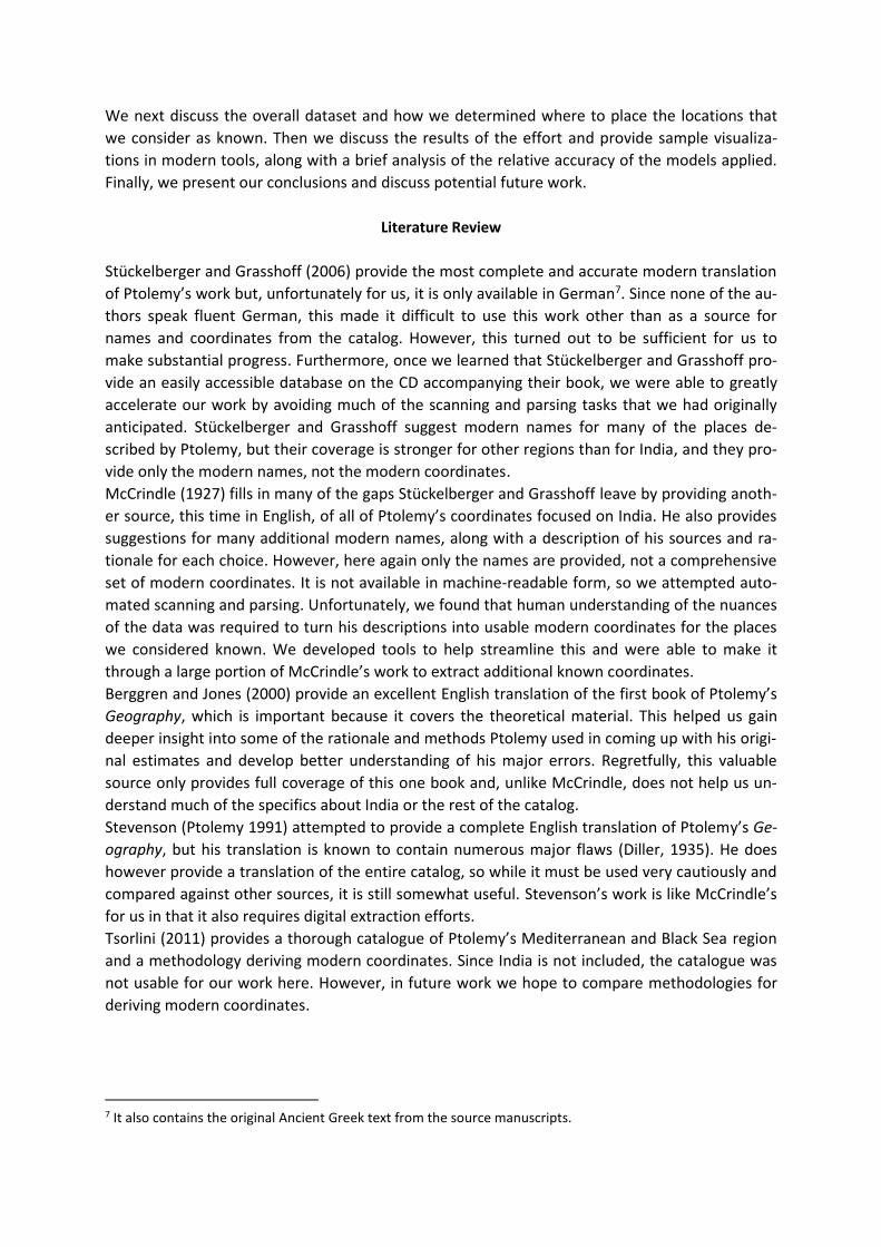
This paper reports on our results achieved so far, with Figure 1 providing a visual representation.

The initial work presented here focuses on India, which corresponds to Book 7 of Ptolemy’s

work, especially Chapters 1 and 4. Our eventual goal is publication of a comprehensive modern

version of Ptolemy’s catalog that will provide either exact or approximate modern coordinates

for every place for which Ptolemy gives us ancient coordinates. By providing such a dataset and

corresponding GIS assets, we will enable exploration and visualization of the ancient world in

ways that are currently not possible.

This paper is organized as follows. First we review the literature we explored including the sur-

viving translations of Ptolemy’s work and their associated commentary. Next we discuss our

tools and workflow and how it supports our effort. After that we discuss the models we applied

to the places for which we do have modern coordinates to predict the coordinates of the others.

Figure 1. This figure provides a rendering of our combined known and unknown loca-

tions from Ptolemy’s Geography using the triangulation approach. The labels shown are

the original Ptolemy names as translated into German by Stückelberger and Grasshoff.

Odoka

Poduke

IoganaModuttu

Spatana

Nakaduma

UlispadaMordula Nubartha

Talakori*

Pati-Golf

Korkobara

Anubingara

Nördliches Kap

Nördliches Kap

AburBere

Kuba

Inde

Sora

Kosa

Iatur

MagurEikur

Gange

Anara

Agara

Ostha

Xoana

Piska

Azika

Semne

Nitra

Dunga

Barake

Ikarta

Polëur

Karige

KaliurPasagePalura

Tabaso

Tagara

Kastra Dosara

Ozoana

Sageda

Soara Nasika

Ozene*

Sydros

Asinda

Tiausa

KoankaSagala

Kindia

Toana

Konta

ArdoneIomusa

Taxila

PaluraKokala

Mapura

Kottis

Bakare

Kamani

Kalliga

Malanga

Tangala

Subuttu

Opotura

Sibrion

Panassa

Bridama

Xodrake

Kodrana

Sabana

Tamasis

Sannaba

MargaraDaidala

Labokla

Poklais

Kosamba

Sippara

Koddura

Melange

Suppara

Kerauge

Gamaliba

Deopalli

Sigalla

Aspathis

Maleiba

Tiatura

Kamigara

Orbadaru

Sarbana

Patala*

Pasipeda

Banagara

Artoarta

AdisdaraPersakra

Amakatis

Arispara

Minagara

Palura*

Kottiara

Armagara

Simylla*

Pulipula

NusaripaSyrastra

Peperine

Bardamana

PikendakaMusopalle

Olochoira

Baithana*

Manipalla

Kartasina

Kartinaga

AsthaguraBardaotis

Patistama

Antachara

Xerogerei

Auxoamis

Barbarei*

Asigramma

Andrapana

Liganeira

Ithaguros

Allosigne

Byzantion

Mandagora

Heptanesia

Banauasei

Bammogura

Nagaruraris

Agrinagara

Pardabathra

Pentagramma

Bukephala*

Kantakosyla

Kap Komaria

Monoglosson

Palimbothra*

Tisapatinga

Ostobalasara

Soas-Quellen

Dionysopolis

Tynas-Mündung

Indus-MündungIndus-Mündung

Indus-Mündung

Ganges-Mündung Antibole-Mündung

Narmades (Aufteilung zum Fluss Mophis)

Ganges (Abzweigung zur Antibole-Mündung)

Copyright:© 2014 Esri

100°0'0"E

100°0'0"E

90°0'0"E

90°0'0"E

80°0'0"E

80°0'0"E

70°0'0"E

70°0'0"E

60°0'0"E

60°0'0"E

30°0'0"N 30°0'0"N

20°0'0"N 20°0'0"N

10°0'0"N 10°0'0"N

Legend

Island of Taprobane (7.04)

India within the Ganges (7.01)

World Shaded Relief

Ptolemy's India

We next discuss the overall dataset and how we determined where to place the locations that

we consider as known. Then we discuss the results of the effort and provide sample visualiza-

tions in modern tools, along with a brief analysis of the relative accuracy of the models applied.

Finally, we present our conclusions and discuss potential future work.

Literature Review

Stückelberger and Grasshoff (2006) provide the most complete and accurate modern translation

of Ptolemy’s work but, unfortunately for us, it is only available in German7. Since none of the au-

thors speak fluent German, this made it difficult to use this work other than as a source for

names and coordinates from the catalog. However, this turned out to be sufficient for us to

make substantial progress. Furthermore, once we learned that Stückelberger and Grasshoff pro-

vide an easily accessible database on the CD accompanying their book, we were able to greatly

accelerate our work by avoiding much of the scanning and parsing tasks that we had originally

anticipated. Stückelberger and Grasshoff suggest modern names for many of the places de-

scribed by Ptolemy, but their coverage is stronger for other regions than for India, and they pro-

vide only the modern names, not the modern coordinates.

McCrindle (1927) fills in many of the gaps Stückelberger and Grasshoff leave by providing anoth-

er source, this time in English, of all of Ptolemy’s coordinates focused on India. He also provides

suggestions for many additional modern names, along with a description of his sources and ra-

tionale for each choice. However, here again only the names are provided, not a comprehensive

set of modern coordinates. It is not available in machine-readable form, so we attempted auto-

mated scanning and parsing. Unfortunately, we found that human understanding of the nuances

of the data was required to turn his descriptions into usable modern coordinates for the places

we considered known. We developed tools to help streamline this and were able to make it

through a large portion of McCrindle’s work to extract additional known coordinates.

Berggren and Jones (2000) provide an excellent English translation of the first book of Ptolemy’s

Geography, which is important because it covers the theoretical material. This helped us gain

deeper insight into some of the rationale and methods Ptolemy used in coming up with his origi-

nal estimates and develop better understanding of his major errors. Regretfully, this valuable

source only provides full coverage of this one book and, unlike McCrindle, does not help us un-

derstand much of the specifics about India or the rest of the catalog.

Stevenson (Ptolemy 1991) attempted to provide a complete English translation of Ptolemy’s Ge-

ography, but his translation is known to contain numerous major flaws (Diller, 1935). He does

however provide a translation of the entire catalog, so while it must be used very cautiously and

compared against other sources, it is still somewhat useful. Stevenson’s work is like McCrindle’s

for us in that it also requires digital extraction efforts.

Tsorlini (2011) provides a thorough catalogue of Ptolemy’s Mediterranean and Black Sea region

and a methodology deriving modern coordinates. Since India is not included, the catalogue was

not usable for our work here. However, in future work we hope to compare methodologies for

deriving modern coordinates.

7 It also contains the original Ancient Greek text from the source manuscripts.

Tools and Workflow

We developed a number of tools and techniques in this work that may be useful to other re-

searchers. This section describes these tools and associated workflow organized as five distinct

functional areas: scanning, data import, KML generation, geocoding, and visualization.

Scanning

Given the data-intensive nature of our problem, one challenge we faced was in scanning and

parsing the various source texts we needed to use. To this end, we developed automated work-

flows based on Tesseract (Smith 2007) and ABBYY FineReader (ABBYY 2015), scanners and scan-

ner automation libraries, and custom parsers to extract data tables from raw recognized text.

While this added some value early on in our process, we eventually determined that the ma-

chine-readable database included by Stückelberger and Grasshoff was sufficient for our initial

work. We need future improvements in this area, as there are tables and other data in source

texts such as McCrindle that we would like to incorporate into our algorithms and make availa-

ble for easy reference in our output and visualization tools.

Data Import

We developed software to read the data on the Stückelberger and Grasshoff CD into our algo-

rithms. Stückelberger and Grasshoff provide four main data files: places, categories, people, and

realities; however, so far we only need places and, to some degree, categories for our work.

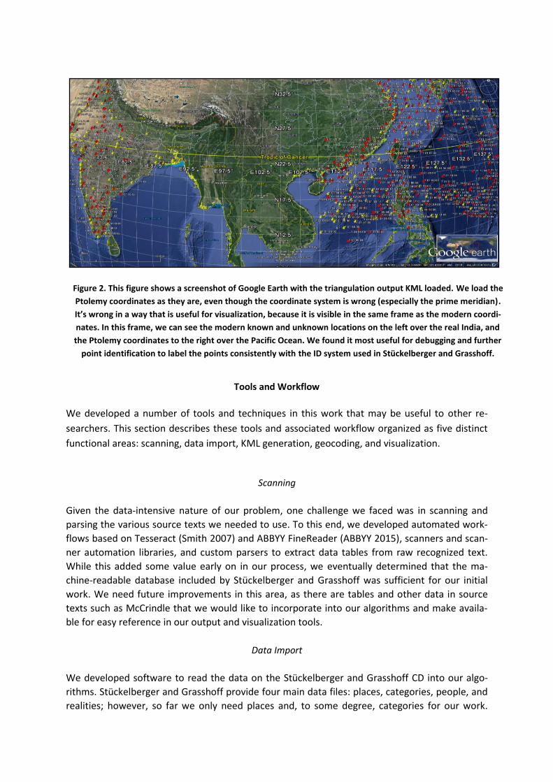
Figure 2. This figure shows a screenshot of Google Earth with the triangulation output KML loaded. We load the

Ptolemy coordinates as they are, even though the coordinate system is wrong (especially the prime meridian).

It’s wrong in a way that is useful for visualization, because it is visible in the same frame as the modern coordi-

nates. In this frame, we can see the modern known and unknown locations on the left over the real India, and

the Ptolemy coordinates to the right over the Pacific Ocean. We found it most useful for debugging and further

point identification to label the points consistently with the ID system used in Stückelberger and Grasshoff.

Translation remains a challenge for us here. Like the book, the data on the CD is all in German.

Even as we would prefer it to be in English, we recognize that for any language we choose for

our output many members of our international audience would face a similar problem. There-

fore, in addition to translating the data from German to English, we also intend to make our re-

sults available in as many other languages as possible. Other internationalization issues, such as

determining the correct file encodings for reading, were worked through somewhat painfully

and taught us to take special precautions as we move towards publishing our data.

KML Generation

Since one of our stated goals with this research is making Ptolemy’s work available in Google

Earth and related tools, we developed several routines to help us produce KML files from the

data. In addition to needing these files as deliverables for our project, we found them invaluable

for our own research tasks including identification of known locations, validation of scanning and

parsing output, and better understanding and verification of mathematical models. An example

of its use is shown in Figure 2. One of the primary libraries we used during our work was sim-

plekml (Lancaster, 2014), which worked well for us initially, but created challenges later on. We

intend to create a custom KML library specifically tailored to our purposes. This will enable a sig-

nificantly enhanced workflow, allowing us to incorporate a faster and more intuitive edit loop on

manual known point adjustments and inputs from other researchers interested in this area.

Geocoding

As our sources mentioned only the names or descriptions for their modern suggestions for plac-

es described by Ptolemy as opposed to the actual modern coordinates, we needed another tool-

set to help us convert those names into coordinates that we could use to feed our algorithms.

We developed two such tools. The first was a program to take in an ID8 and a place name, inter-

face with the Google Geocoding API (Google, 2015) for the actual geocoding, and output a file

containing modern coordinates for that place name that could be referenced during later pro-

cessing for that ID. The second was a program that generated the same files, but did so by

providing us with a minimal GUI to allow us to manually find the locations on a map and copy

them over or input them by hand. Both tools could still use some improvements, but saved us

countless hours in collecting the data to feed our models.

Visualization

Google Earth was a key focus of our effort and became a primary visualization tool for us. The

KML generation and Google Earth import steps we built into our workflow were essential to our

rapid progress. In addition, two other visualization tools we used are also worth mentioning. The

first is Google Maps because of its usefulness in helping determine where the harder to find sug-

gested modern place names might actually be located and looking up their specific coordinates

manually. This included tasks such as tracing rivers from mouth to source to match the reference

points mentioned by Ptolemy. The second is a custom animation that interpolated all points

from their Ptolemy location to their modern equivalents.

8 We adopted Stückelberger and Grasshoff’s Ptolemy ID labeling method.

Visualization became essential in helping us understand our models, identify outliers and errors

in our geocoding process, and envision new models. A screenshot of our visualization program in

action is shown in Figure 3.

Places

Ptolemy’s Geography is a unique ancient work, and identifying the modern equivalent of even a

single place mentioned in its catalog can be extremely difficult sometimes. Even for known plac-

es, there are often several reasonable modern candidates available in the literature, each with

its compelling rationale, and with alternatives being hundreds of kilometers apart. In this sec-

tion, we provide more information about Ptolemy’s Geography, the data that we used to seed

our set of known modern equivalents, and our efforts to identify additional known data points to

use for predicting where the other data points fall.

About Ptolemy’s Geography

Ptolemy’s Geography is comprised of several books. The first book describes prior work by other

scholars of his time and his improvements to that work along with his own novel contributions.

Book 2 begins the catalog part and each subsequent book up to and including Book 7 focuses on

a different area of the known world at that time. Because our focus is on India, we primarily in-

vestigated Book 7 for the India portion of the catalog, and Book 1 for theoretical underpinnings.

Book 7 is comprised of four chapters, each pertaining to a different region of southern Asia.

Chapter 1 is by far the largest and focuses on the Indian subcontinent spanning from modern

Pakistan, including the area around the Indus River, to all around the coastline of India, and

along Ganges River and the Himalayas to where the Ganges enters the sea. Chapter 2 describes

the area beyond the Ganges River. Chapter 3 describes the areas located even further east than

India. Finally, Chapter 4 describes the island of Taprobane, which is known today as Sri Lanka,

former Ceylon. Of these, for our purposes in focusing on modern India, Chapters 1 and 4 are the

most important.

Within each chapter, Ptolemy follows a consistent pattern to enumerate all the places. First, he

outlines the entire coastal area. Then he lists all the mountain ranges, followed by the sources,

major confluences, bends, and mouths of the major rivers. He then proceeds to list the various

Figure 3. Shown above are the screenshots of the animation visualization sketch in its extreme states. The tool cy-

cles smoothly between ancient and modern coordinates, allowing the eye to follow both the known and unknown

points as they move between their two locations. Users can click on the sketch to take manual control of the time

bar.

people of the land along with their major towns. Finally he lists the surrounding islands.

Stückelberger and Grasshoff’s Database

In the database that accompanies their translation of Ptolemy’s work, Stückelberger and Grass-

hoff list 12,883 unique records in their places table. Of those, 1,217 records pertain to Book 7.

Within that set, 640 records actually have a Ptolemy latitude and longitude associated with

them. Because of the nature of our work, we filtered out all records that lacked coordinates. Of

those that remained, 47 were duplicates by their ID, most of which were there because they rep-

resented either an alternate name, or a larger feature such as a mountain, and each row speci-

fied a different point within the feature. This leaves 593 unique places in Book 7. Stückelberger

and Grasshoff suggest a modern name for 99 of those places, 84 of which are for Chapter 1. Dur-

ing our first pass, we were only able to successfully geocode about 50 of those locations using

our program that leveraged Google’s geocoding API. This was the initial set we took for further

processing to try to derive the other unknown points.

Additional Points

After working with the various models for some time, we realized that we really needed addi-

tional known points. Using a combination of translations of Stückelberger and Grasshoff names

Figure 4. This figure shows the triangulation visualization, depicting especially clearly the Delaunay triangulation

used in selecting which known points for each unknown points would be used for the estimation. The colors are

inconsistent when viewing them all at the same time as in the top figure, but become clear when only a single

triangle is viewed at a time as shown in the bottom figures.

along with McCrindle, Wikipedia, Google searches, and Google Maps, we were able to come up

with potential names and coordinates for 85 more places out of the 593 that we would like to be

able to plot. The 98 known points for Chapter 1 are listed in Table 1, and the 21 points known for

Chapter 4 are listed in Table 2.

Models

While we know some of the modern equivalents of places that Ptolemy describes based on evi-

dence accumulated through the literature, most of them are simply unknown. The challenge we

address with our work is to use the few places whose locations are known through the literature

to estimate the locations of many that remain unknown. This section describes the models we

used to make such estimates.

Linear Regression Model

Like Gusev, Stafeyev and Filatova’s (2005) in their work on Ptolemy’s Africa, one of our models

was a simple linear regression model. We use both ancient latitude and longitude to predict the

modern latitude and then separately use the same input data to predict the modern longitude.

We used the scikit-learn library for Python (Pedregosa 2011) in our implementation9.

The model used is the one described earlier in Gusev, Stafeyev and Filatova: 𝜆𝑚 = 𝑎0 + 𝑎1𝜆𝑝 + 𝑎2𝜑𝑝,

𝜑𝑚 = 𝑏0 + 𝑏1𝜆𝑝 + 𝑏2𝜑𝑝,

where 𝜆𝑚 and 𝜑𝑚 represent the modern longitude and latitude, 𝜆𝑝 and 𝜑𝑝 represent the longi-

tude and latitude mentioned by Ptolemy, and the vectors 𝒂 and 𝒃 are the regression coeffi-

cients.

Triangulation Model

Also originating from Gusev, Stafeyev and Filatova, this method uses three Ptolemy points for

which we know their modern coordinates to form a spherical triangle surrounding a point to be

predicted, and then triangulate to find the unknown point. That is, we estimate the unknown

modern coordinate pair 𝜆𝑚 and 𝜑𝑚 using the formulas

𝜆𝑚 = ∑𝜆𝑖𝑆𝑖

𝑆1 + 𝑆2 + 𝑆3

,

3

𝑖=1

𝜑𝑚 = ∑𝜑𝑖𝑆𝑖

𝑆1 + 𝑆2 + 𝑆3

,

3

𝑖=1

maintaining the notation used earlier, and extending it with 𝜆𝑖 and 𝜑𝑖 as the longitude and lati-

tude of the modern coordinates for the three surrounding points, and 𝑆𝑖 as the surface area for

the spherical sub-triangle across from the unknown point, which is formed by trisecting the out-

er triangle by the lines leading from each of its three vertices to the interior unknown point. Like

9 We use aspects of scikit-learn for other models and tasks in our work as well, but do not proceed to exhaust-ively enumerate them all here.

Gusev, Stafeyev and Filatova, we also compute the area of the spherical triangle 𝑆 mentioned

above as

𝑆 = 4 arctan √tan (𝑠

2) tan (

𝑠 − 𝑎

2) tan (

𝑠 − 𝑏

2) tan (

𝑠 − 𝑐

2)

where 𝑎, 𝑏, and 𝑐 are the lengths of the sides of the triangle in radians, and 𝑠 = (𝑎 + 𝑏 + 𝑐)/2.

Finally, again following Gusev, Stafeyev and Filatova, we use the modified great circle distance to

compute the lengths of the sides of the spherical triangle according to the formula

𝑑1,2 = 2 arcsin [min {(sin|𝜑1 − 𝜑2|

2)

2

+ cos 𝜑1 cos 𝜑2 (sin𝛾|𝜆1 − 𝜆2|

2)

2

}] ,

where, like before, 𝜆 and 𝜑 represent the longitude and latitude of the two points, and a nar-

rowing coefficient of 𝛾 is applied to account for the local longitudinal stretch of Ptolemy coordi-

nates.

Note the constraint that each of the unknown places to be predicted must be enclosed by a

spherical triangle of other points that we do know. We found that many unknown locations do

not satisfy that criteria, so this model fails to estimate modern coordinates for a significant por-

tion of the catalog. Furthermore, this constraint makes it quite difficult to test and validate the

model, because many of the known points that we’d want to validate are on the convex hull, so

removing them makes it impossible to estimate their modern locations, and thereby impossible

to measure predictive accuracy for them.

However, for the remaining points, and after substantial manual effort to find additional known

points along the convex hull of the dataset, this approach turned out to be the most accurate of

those we have researched, and seemed the most conceptually straightforward.

Another noteworthy challenge not addressed by Gusev, Stafeyev and Filatova was how to assign

the set of unknown points to the sets of points representing their respective surrounding spheri-

cal triangles. To address this challenge in an efficient way we computed a Delaunay (1934) trian-

gulation of the known points in their ancient coordinates and looked up the surrounding points

for a point to be predicted by querying the results.

Basis Vector Model

This model attempts to relax the surrounding triangle constraint, but the price appears to be

highly variant results. We find the three nearest known neighbors for each location to be pre-

dicted based on their distance to the unknown and then treat them as a basis vector as men-

tioned by Strang (2009) of the unknown in ancient coordinate space. We use these to construct

a matrix 𝐴 representing the basis

[𝜆3 − 𝜆1 𝜆2 − 𝜆1

𝜑3 − 𝜑1 𝜑2 − 𝜑1].

We then take the Ptolemy coordinates for the unknown point, 𝜆4 and 𝜑4 to form a vector 𝒃 as

[𝜆4 − 𝜆1

𝜑4 − 𝜑1].

We use these to solve for a vector 𝒙 in

𝐴𝒙 = 𝒃 representing the unknown point in terms of the basis formed by the known points.

We form a second basis and the associated matrix 𝐵 using our modern coordinates for the

known points and solve

𝐵𝒙 = 𝒄

for the vector 𝒄, which represents the modern equivalent of the unknown location in terms of

the modern basis. We compute the estimated modern coordinates for the unknown point as

[𝜆𝑚

𝜑𝑚] = [

𝜆1

𝜑1] + [

𝑐𝜆

𝑐𝜑].

Bayesian Adjustment

The technique developed in this section is not a model on its own. Rather, it takes the output of

any of the other models and adjusts it to account for certain prior beliefs, such as that places

described by Ptolemy as situated on mainland should fall somewhere on the land mass repre-

senting India.

Specifically, we create an image representing the map of India that is black and white, with black

representing areas of zero probability and white representing areas of a uniformly distributed

probability over the entire subcontinent. This map is loaded as a grid approximation of the prob-

ability, normalized so that the entire image (i.e., the grid of probabilities) sums to one. We then

take each of the output points and create a second grid probability approximation that treats the

output point as the mean of a bivariate normal distribution. We use what Kruschke (2011) shows

us about how to infer a binomial proportion via grid approximation to apply Bayes rule

𝑃(𝐴|𝐵) =𝑃(𝐴)𝑃(𝐵|𝐴)

𝑃(𝐵),

combining the prior with the data and normalizing to arrive at a posterior belief for the new

point. For us, 𝑃(𝐴|𝐵) is the posterior grid we are interested in, containing the probability distri-

bution of our belief of the new location of the point. The prior 𝑃(𝐴) is our belief in where the

point must lie without regard to our new data, which for us is the land mass of the Indian sub-

continent as represented by the black and white map of India. The new data 𝑃(𝐵|𝐴) we take as

the output from our input model, a bivariate normal grid representation. The evidence 𝑃(𝐵)

given our grid approach is the value the causes our grid to be a probability distribution by sum-

ming to 1, which is the sum of the entire grid.

We then take the maximum a-posteriori (MAP) of the resulting grid approximation posterior as

the new output point. We deemed this approach superior to the maximum likelihood estimator

(MLE) for our purposes, because with the latter we still occasionally end up with points in the

middle of the ocean. The MAP does not suffer from this, because the point has to have some

probability to survive as the MAP. But the points in the ocean are treated as zero probability in

our prior, so they have zero probability in the posterior as well. The prior, along with the data

and posterior as interim images are shown in Figure 6. We intend to extend this approach to ap-

ply our beliefs around other features such as rivers, lakes, and mountains to our other models.

For instance, we could similarly load a prior with a grid approximation of a river such as the Gan-

ges to help adjust points describing towns that are described by Ptolemy as near it. The nature of

Ptolemy’s descriptions and approach will lend itself well to this adjustment.

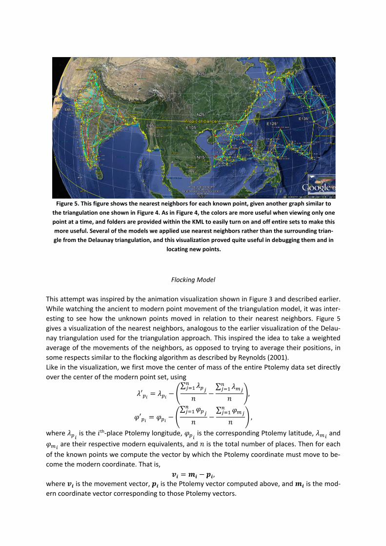
Flocking Model

This attempt was inspired by the animation visualization shown in Figure 3 and described earlier.

While watching the ancient to modern point movement of the triangulation model, it was inter-

esting to see how the unknown points moved in relation to their nearest neighbors. Figure 5

gives a visualization of the nearest neighbors, analogous to the earlier visualization of the Delau-

nay triangulation used for the triangulation approach. This inspired the idea to take a weighted

average of the movements of the neighbors, as opposed to trying to average their positions, in

some respects similar to the flocking algorithm as described by Reynolds (2001).

Like in the visualization, we first move the center of mass of the entire Ptolemy data set directly

over the center of the modern point set, using

𝜆′𝑝𝑖= 𝜆𝑝𝑖

− (∑ 𝜆𝑝𝑗

𝑛𝑗=1

𝑛−

∑ 𝜆𝑚𝑗𝑛𝑗=1

𝑛),

𝜑′𝑝𝑖= 𝜑𝑝𝑖

− (∑ 𝜑𝑝𝑗

𝑛𝑗=1

𝑛−

∑ 𝜑𝑚𝑗𝑛𝑗=1

𝑛) ,

where 𝜆𝑝𝑖 is the 𝑖th-place Ptolemy longitude, 𝜑𝑝𝑖

is the corresponding Ptolemy latitude, 𝜆𝑚𝑖 and

𝜑𝑚𝑖 are their respective modern equivalents, and 𝑛 is the total number of places. Then for each

of the known points we compute the vector by which the Ptolemy coordinate must move to be-

come the modern coordinate. That is,

𝒗𝒊 = 𝒎𝒊 − 𝒑𝒊,

where 𝒗𝒊 is the movement vector, 𝒑𝒊 is the Ptolemy vector computed above, and 𝒎𝒊 is the mod-

ern coordinate vector corresponding to those Ptolemy vectors.

Figure 5. This figure shows the nearest neighbors for each known point, given another graph similar to

the triangulation one shown in Figure 4. As in Figure 4, the colors are more useful when viewing only one

point at a time, and folders are provided within the KML to easily turn on and off entire sets to make this

more useful. Several of the models we applied use nearest neighbors rather than the surrounding trian-

gle from the Delaunay triangulation, and this visualization proved quite useful in debugging them and in

locating new points.

For prediction, we take the 𝑘 nearest neighbors of the unknown point 𝑦𝑝, use their respective

distances to compute weighted average of the movement, and use the obtained average to

move the unknown point so that it becomes its modern point

𝑦𝑚 = 𝑦𝑝 + ∑ 𝑣𝑖𝑤𝑖

𝑘

𝑖=1

where y is the predicted point vector 𝜆𝑚 and 𝜑𝑚, 𝑣𝑖 is the difference of the 𝑖th nearest neighbor

of 𝑦’s 𝑘 neighbors of its modern coordinate to its Ptolemy coordinate, and 𝑤𝑖 is the weight for

the 𝑖th neighbor. The weight for each neighbor is computed as

𝑤𝑖 =𝑑𝑖

∑ 𝑑𝑗𝑘𝑗=1

.

Unsuccessful Models

Two additional attempts were made at breaking free of the triangulation constraint. The first of

the resulting methods we called our multilateration approach. It sought to adopt techniques

used by modern GPS technologies, locating a point based on its relative spherical distance from

3 other known points. We constructed spheres based on the modern coordinates and found

their intersection, using an SVD based method we found on Stack Overflow (zerm 2011). We do

not elaborate further, as we found the overall approach complex and ineffective. However, as

we later identified several important flaws in our attempt, we may revisit it later.

We called our second method the tri-area approach. We intended to enhance the triangulation

model by removing the constraint that the unknown points had to be fully enclosed. The idea

was based on what turned out to be a misunderstanding about the way the triangulation ap-

proach actually works. We mistakenly thought that after applying the weights to compute the

new points, the ratios of the areas of the triangles would be preserved in the new configuration.

Unfortunately, this is not true; applying the weighted average does not preserve the ratios of the

areas. While we were successful in creating a solution that does seem to preserve the areas of

the triangles, it does not appear to match up at all with the previous triangulation approach. We

also found this approach ineffective and do not consider it further here.

Figure 6. The leftmost figure shows the prior we used for India (book 7, chapter 1). The other figures show the rest

of the Bayesian calculation. The prior is on the left, the data is in the center, and the posterior is on the right. We

take the MAP of the posterior as the adjusted point.

Results

Google Earth

This was our primary output, especially given how much we made use of it. We found KML to be

remarkably powerful, despite its simplicity, in communicating our visualization needs to Google

Earth and found the tool to support our workflow well in trying to determine new points to con-

sider as known.

In addition to visualizing the points, we also found it incredibly useful to visualize other geomet-

ric artifacts from our models. For instance, the triangulation approach relies heavily on the De-

launay triangulation. Visualization of this triangulation, along with the points that comprise it

and the points that fall within each triangle, proved to be quite useful in improving both the

model and the data. An example of this visualization is shown in Figure 4.

Processing Visualization

This was a useful visualization for understanding which points moved where, and how the

movements compared with one another. It was the inspiration for the flocking model. This tool

was developed as a Processing sketch (Raes 2007). Screenshots of the visualization in its two ex-

treme states are given in Figure 3.

Figure 7. This figure shows the error computed for leave-one-out validation for our two strongest mathematical

models: triangulation and flocking. The data has been sorted in decreasing order of the triangulation error. We

can see here that the flocking error seems to follow roughly along with the triangulation error, but that there is a

high degree of variance along the line, indicating that for some points flocking does better, while for others tri-

angulation does better.

-

100.00

200.00

300.00

400.00

500.00

600.00

1 4 7 10 13 16 19 22 25 28 31 34 37 40 43 46 49 52 55 58 61 64 67 70 73 76 79

Erro

r (m

iles)

Location row number (with rows ordered by decreasing triangulation error)

Ptolemy error comparison: triangulation vs. flocking

triangulation error flocking error

Error Analysis

We conducted leave-one-out validation and cross-validation on the two models we found to be

most accurate, after applying our Bayesian adjustment to each, for Book 7 Chapter 1, which co-

vers most of modern India, which Ptolemy describes as the intra-Ganges. We were only able to

compare for regions that were not excluded by the triangulation constraint described earlier in

this paper. Our average error for the flocking approach was 145 miles, and our average triangu-

lation error was 132 miles. Figure 7 allows us to visualize how the two models are each more ac-

curate for some points than others. That is, because the plot is sorted by decreasing error on the

triangulation approach, the high degree of change shown in the series for the flocking approach

means that it was less accurate than triangulation in some cases and more accurate in others.

Furthermore, we can also see that as this happens, the two do follow the same trend, with over-

all error decreasing for flocking as it decreases for triangulation.

Conclusions and Future Work

Our hope is that this work will stimulate future research interest in this area and serve as a use-

ful foundation for such work. In the rest of this section, we give some recommendations for fu-

ture projects in this area.

The first and most obvious extension is to simply apply the same concepts and techniques to

each of the other books and chapters in Ptolemy’s Geography. We focused on India to get start-

ed, but the same principles and techniques should work just as well for any of the other regions.

In fact, it is likely that other regions may have far better results, because Ptolemy knew those

areas better and greater percentages of Ptolemaic places may turn out to be known.

The next extension is to further improve on the known locations within India. We recognize that

there is still a degree of uncertainty in respect of many of the places we are classifying as known,

and additional work in this area could reduce that amount of uncertainty. A dream scenario

would be for archaeologists to travel to the coordinates we provide and find a lost ancient city

mentioned by Ptolemy.

Also, we are not doing anything yet to effectively capture the degree to which we consider each

place known, while clearly we know some locations with a higher degree of certainty than oth-

ers. Adopting a rating-like discrete classification of the degree to which each point is known

could be useful. We could even go further and describe a full prior distribution for each known,

fully capturing our beliefs about its certainty. We already use this concept in our Bayesian ad-

justment, but it could be utilized to a much greater degree in future work.

We also recognize that the models we developed leave ample opportunity for improvements

along several dimensions. For example, we could substantially extend the amount of data we

use. The only data we are using in terms of features for prediction are the Ptolemy latitude and

longitude. It is worth exploring other potential feature data such as toponym information, tribe

names, metadata such as more detailed category information, and further geological feature

information. For instance, for mountain identification it may be possible to make use of eleva-

tion data to predict more likely coordinates for mountain ranges. Similarly, vector data for river

paths could potentially be used to better locate various river-related features, towns and other

places that are described in terms of their proximity to such rivers. Other dimensions might in-

clude type of model used and applying combinations of models.

We anticipate that many of the tools and techniques described in this paper would be useful in

understanding other ancient authors. Indeed, we intend to carry the work through the rest of

Ptolemy’s Geography, providing a complete modern rendition of his oikoumene in tools like

Google Earth, Google Maps, and ArcGIS.

The source code for the tools developed in this work is available on GitHub10.

Acknowledgments

This work was partially supported by Google Geo Education Award and Google Maps Engine Grant.

10 https://github.com/coreyabshire/ptolemy

References

ABBYY. (2015). Try OCR software from ABBYY: text recognition software for Windows and Mac. In digital form, http://finereader.abbyy.com/.

Berggren J. and A. Jones (2000). Ptolemy's Geography: An annotated translation of the theoreti-cal chapters. Princeton, NJ: Princeton University Press.

Delaunay, B. (1934). Sur la sphère vide. Izvestia Akademii Nauk SSSR, Otdelenie Matematicheskii i Estestvennykh Nauk 7: 793-800.

Diller, A. (1935). Review of Stevenson’s translation. Isis 22 (2): 533-539. In digital form, http://penelope.uchicago.edu/Thayer/E/Journals/ISIS/22/2/reviews/Stevensons_Ptolemy*.html

Google. (2015). The Google Geocoding API. In digital form, https://developers.google.com/maps/documentation/geocoding/.

Gusev D. A., S. K. Stafeyev, L. M. Filatova (2005). Iterative reconstruction of Ptolemy’s West Afri-ca. The 10th International Conference on the Problems of Civilization. Moscow: RosNOU.

Kruschke, J. (2011). Doing Bayesian data analysis: A tutorial with R and BUGS. New York, NY: Ac-ademic Press.

Lancaster, K. (2014). Overview - simplekml 1.2.5 documentation. In digital form, https://simplekml.readthedocs.org/en/latest/

McCrindle, J. W. (1927). Ancient India as described by Ptolemy. New Delhi: Munshiram Manohar-lal Publishers Pvt. Ltd.

Pedregosa, F., et al. (2011). Scikit-learn: Machine learning in Python. Journal of Machine Learning Research 12: 2825-2830.

Ptolemy, C. (1991). Claudius Ptolemy, The Geography, Translated and edited by E.L. Stevenson. New York, NY: Dover Publications, Inc.

Raes C., B. Fry, J. Maeda (2007). Processing: A programming handbook for visual designers and artists. Cambridge, MA: The MIT Press.

Reynolds, C. (2001). Boids: background and update. In digital form, http://www.red3d.com/cwr/boids/.

Schoff, W. H. (1912). Periplus of the Erythraean Sea: Travel and Trade in the Indian Ocean by a Merchant of the First Century, Translated from the Greek and Annotated. New York, NY: Long-mans, Green, and Co.

Smith, R. (2007). An overview of the Tesseract OCR Engine. ICDAR '07 Proceedings of the Ninth International Conference on Document Analysis and Recognition. Washington, DC: IEEE Comput-er Society.

Strang, G. (2009). Introduction to Linear Algebra. Fourth edition. Wellesley, MA: Wellesley-Cambridge Press.

Stückelberger A. and G. Grasshoff (2006). Klaudios Ptolemaios: Handbuch der Geographie, Griechisch-Deutsch. Basel: Schwabe Verlag.

Tsorlini, A. (2011). Claudius Ptolemy “Geōgrafikē Yfēgēsis” (Geographia): digital analysis, evalua-tion, processing and mapping the coordinates of Greece, the Mediterranean and the Black Sea, based on 4 manuscripts and 15 printed editions, from Vaticanus Urbinas Gr. 82 (13th cent.) until today : the new Catalogue “GeoPtolemy- θ”. In digital form, http://digital.lib.auth.gr/record/128272

zerm (2011). Multilateration of GPS Coordinates. In digital form, http://stackoverflow.com/questions/8318113/multilateration-of-gps-coordinates.

Tables

Table 1. Modern coordinates for known locations in Book 7 Chapter 1. Ptolemy ID Ptolemy Name Modern Name Ptol. Lat. Ptol. Lon. Mod. Lat. Mod. Lon.

7.01.02.04 Indus-Mündung (westlichste) 19.83 110.33 24.74 67.55

7.01.02.10 Indus-Mündung 20.25 113.33 23.77 68.61

7.01.03.01 Bardaxema Bhadreshwar 20.67 113.67 21.64 69.63

7.01.03.02 Syrastra Junagadh 19.50 114.00 21.17 72.83

7.01.03.03 Monoglosson Mangrol 18.67 114.17 21.12 70.12

7.01.04.02 Mophis-Mündung Mahi 18.33 114.00 22.24 72.66

7.01.05.03 Narmades-Mündung Narmada 16.75 112.00 21.61 72.56

7.01.05.04 Nusaripa Navsari 16.50 112.50 20.95 72.95

7.01.05.05 Pulipula Sanjan 16.00 112.50 20.19 72.82

7.01.06.02 Suppara Sopara 15.50 112.17 19.42 72.80

7.01.06.03 Goaris-Mündung UlhasRiv-er/VasaiCreek

15.17 112.25 19.32 72.80

7.01.06.05 Bindas-Mündung Thanecreek 15.00 110.50 19.05 72.98

7.01.06.06 Simylla Chaul 14.75 110.00 18.57 72.94

7.01.06.07 Balepatna Dabhol 14.33 111.50 17.59 73.18

7.01.06.08 Hippokura Goregaon(West) 14.00 111.75 19.16 72.84

7.01.07.02 Mandagora Mandangarh 14.17 113.00 17.98 73.25

7.01.07.03 Byzantion Vijayadurg 14.67 113.67 16.55 73.34

7.01.07.05 Nanagunas-Mündung Taptiriv-er/Haziracreek

13.83 114.50 21.07 72.68

7.01.07.07 Nitra Manga-lore/Mangaluru

14.67 115.50 12.91 74.84

7.01.08.02 Tyndis Ponnani 14.50 116.00 10.77 75.93

7.01.08.04 Kap Kalaikarias Chalakudy 14.00 116.67 10.31 76.33

7.01.08.05 Muziris Cranganur 14.00 117.00 10.22 76.20

7.01.08.06 Pseudostomos-Mündung

Periyar-Mündung 14.00 117.33 10.18 76.16

7.01.08.10 Bakare Pirakkad 14.50 119.50 10.06 76.46

7.01.08.11 Baris-Mündung Pamba 14.33 120.00 9.31 76.38

7.01.09.02 Nelkynda Nirkunnam 14.33 120.33 9.41 76.35

7.01.09.06 Kap Komaria KapComorin 13.50 121.75 8.09 77.54

7.01.10.05 Kolchoi Korkei 15.00 123.00 8.63 78.07

7.01.10.06 Solen-Mündung Tamraparni-Mündung

14.67 124.00 8.63 78.11

7.01.11.03 Kap Kalligikon PointCallimere 13.33 125.67 9.29 79.31

7.01.13.02 Chaberis Tranquebar 15.75 128.33 11.03 79.85

7.01.14.02 Poduke Virampatnam 14.75 130.25 11.89 79.82

7.01.15.06 Ablegeplatz zur Goldenen Chersones 11.00 136.33 18.16 83.78

7.01.17.05 Adamas-Mündung Subarnarekha-Mündung

18.00 142.67 21.56 87.37

7.01.18.07 Antibole-Mündung 18.25 148.50 22.07 89.94

7.01.27.01 Indus (Zusammenfluss mit dem Koas)

In-dus(ZusammenflussmitdemKonar)

31.00 124.50 33.92 72.23

7.01.27.02 Koas (Zusammenfluss mit dem Suastos)

Konar(ZusammenflussmitdemSwat)

31.67 122.50 34.11 71.71

7.01.27.03 Indus (Zusammenfluss mit dem Zaradros)

In-dus(ZusammenflussmitdemSutlej)

30.00 124.00 29.15 70.72

7.01.27.07 Bidaspes (Zusammenfluss mit dem Sanda-bal)

32.67 126.67 31.17 72.15

7.01.33.02 Pseudostomos (Biegung)

Periyar 17.25 118.50 9.58 77.11

7.01.34.03 Solen-Quellen im Bet-tigo-Gebirge

Tamraparni-QuellenindenS-Ghats

20.50 127.00 8.69 77.36

7.01.34.04 Solen (Biegung) Tamraparni 18.00 124.00 8.69 77.68

7.01.43.04 Dionysopolis 32.50 121.50 34.43 70.32

7.01.44.04 Poklais Charsadda 33.00 123.00 34.15 71.74

7.01.45.05 Taxila Taxila 32.25 125.00 33.74 72.80

7.01.46.04 Euthydemia Sialkot 32.00 126.67 32.49 74.53

7.01.48.03 Labokla 33.33 128.00 31.56 74.36

7.01.48.04 Batanagra 33.33 130.00 29.58 74.32

7.01.49.05 Indabara 30.00 127.25 28.61 77.25

7.01.50.01 Modura Mathura 27.17 125.00 27.49 77.67

7.01.50.02 Gagasmira 27.50 126.67 28.61 76.66

7.01.50.03 Erarassa 26.00 123.00 25.32 82.98

7.01.51.04 Konta 34.33 133.50 25.72 81.52

7.01.51.05 Margara 34.00 135.00 27.74 78.57

7.01.51.06 Batankaisara 33.33 132.67 29.96 76.82

7.01.59.01 Patala Hyderabad 21.00 112.83 25.39 68.37

7.01.59.02 Barbarei Bhambore 22.50 113.25 24.75 67.52

7.01.60.03 Auxoamis Ajmer 22.33 115.50 26.45 74.64

7.01.60.04 Asinda Siddhpur,Gujarat,India

22.00 114.25 23.92 72.37

7.01.60.05 Orbadaru Mt.Abu 22.00 115.00 24.59 72.71

7.01.60.06 Theophila Devaliya 21.17 114.25 23.03 70.00

7.01.60.07 Astakapra Hathab 20.25 114.67 21.57 72.27

7.01.61.01 Panassa notownthere 29.00 122.50 28.78 70.10

7.01.61.03 Naagramma Naushehra 27.00 120.00 32.57 72.15

7.01.61.04 Kamigara Sukkur 26.33 119.00 27.71 68.85

7.01.61.05 Binagara Brahmanabad 25.33 118.00 25.88 68.78

7.01.62.04 Barygaza Bharuch 17.33 113.25 21.71 73.00

7.01.63.01 Agrinagara AgarMalwa 22.50 118.25 23.71 76.01

7.01.63.05 Xerogerei Dhar 19.83 116.33 22.60 75.30

7.01.63.06 Ozene Ujjain 20.00 117.00 23.18 75.78

7.01.63.10 Nasika Nasik 17.00 114.00 20.00 73.79

7.01.69.03 Stagabaza Bhojapur 28.50 133.00 19.68 74.04

7.01.69.04 Bardaotis Bharhut 28.50 137.50 24.45 80.88

7.01.70.02 Bridama Bilhari 27.50 134.50 23.14 79.97

7.01.70.03 Tholobana Bahoriband 27.00 136.33 23.67 80.07

7.01.71.05 Panassa Panna 24.50 137.67 24.72 80.18

7.01.73.01 Sambalaka Sambhal 29.50 141.00 28.59 78.57

7.01.73.03 Palimbothra Patna 27.00 143.00 25.61 85.14

7.01.73.04 Tamalites Tamluk 26.50 144.50 22.30 87.92

7.01.76.05 Ozoana Seoni 20.50 138.25 22.09 79.54

7.01.78.01 Kartinaga Karnigar 23.00 146.00 22.51 87.36

7.01.78.02 Kartasina Berhampur 21.67 145.50 19.31 84.79

7.01.82.06 Baithana* Paithan 18.17 117.00 19.48 75.38

7.01.83.12 Modogulla Mudgal 18.00 119.00 16.01 76.44

7.01.83.14 Banauasei Banavasi 16.75 116.00 14.53 75.02

7.01.86.09 Karura Tirukkarur 16.33 119.00 10.77 79.64

7.01.89.06 Modura Madurai 16.33 125.00 9.93 78.12

7.01.91.05 Orthura Uraiyar 16.33 130.00 12.09 79.14

7.01.91.08 Abur 16.00 129.00 12.82 78.63

7.01.92.04 Karige 15.00 132.67 14.47 78.82

7.01.92.06 Pikendaka 14.00 131.50 14.08 77.60

7.01.92.10 Malanga 13.00 133.00 16.70 81.10

7.01.93.03 Bardamana 15.25 136.25 17.97 79.59

7.01.93.06 Pityndra 12.50 135.50 16.56 80.34

7.01.94.03 Barake Beyt 18.00 111.00 22.46 69.10

7.01.95.02 Milizigeris Jaygarh 12.50 110.00 17.29 73.22

7.01.95.03 Heptanesia 13.00 113.00 15.93 73.46

7.01.96.02 Kory Rameswaram 13.00 126.50 9.29 79.31

Table 2. Modern coordinates for known locations in Book 7 Chapter 4.

Ptolemy ID Ptolemy Name Modern Name Ptol. Lat. Ptol. Lon. Mod. Lat. Mod. Lon.

7.04.02.01 Nördliches Kap Point Pedro 12.50 126.00 9.82 80.23

7.04.03.01 Nördliches Kap Point Pedro 12.50 126.00 9.82 80.23

7.04.03.05 Kap Anarismundu 7.75 122.00 8.44 79.85

7.04.03.09 Priapis-Hafen 3.67 122.00 7.19 79.86

7.04.04.03 Kap des Zeus 1.00 120.50 6.93 79.86

7.04.04.07 Odoka (2.00) 123.00 6.15 80.11

7.04.04.08 Kap der Vögel Dondra Head (2.50) 125.00 6.05 80.22

7.04.05.01 Dagana, der Selene heilig

(2.00) 126.00 5.93 80.59

7.04.05.02 Korkobara (2.33) 127.67 6.03 80.79

7.04.05.04 Kap Ketaion (0.67) 132.50 6.36 81.47

7.04.05.08 Mordula 2.33 131.00 6.84 81.83

7.04.06.01 Abaraththa 3.25 131.00 7.38 81.84

7.04.06.02 Helios-Hafen 4.00 130.00 7.72 81.70

7.04.06.06 Kap Oxeia Foul Point 7.50 130.00 8.52 81.32

7.04.06.07 Ganges-Mündung Mahaweli Ganges-Mündung

7.33 129.00 8.46 81.23

7.04.07.01 Nagadiba Nagadeepa Ra-jamaha Vihara

8.50 129.00 9.61 79.77

7.04.07.03 Anubingara 9.67 128.67 8.82 81.10

7.04.07.04 Moduttu 11.00 128.00 8.98 80.94

7.04.07.07 Talakori 11.67 126.33 9.82 80.14

7.04.10.01 Anurogrammon Anuradhapura 8.67 124.17 8.35 80.39

7.04.10.02 Maagrammon Tissamaharama 7.33 127.00 6.28 81.28