Proceedings of the ASME 2009 International Design Engineering Technical Conferences &Computers and Information in Engineering Conference

IDETC/CIE 2009August 30-September 2, 2009, San Diego, USA

DETC2009-86947

A METHOD FOR ESTIMATING PHYSICAL PROPERTIESOF A COMBINED BICYCLE AND RIDER

Jason K. Moore∗Mont Hubbard

Sports Biomechanics LaboratoryDepartment of Mechanical and Aeronautical Engineering

University of CaliforniaOne Shields Avenue

Davis, California 95616Email: jkmoor@ucdavis.edu

mhubbard@ucdavis.edu

J. D. G. KooijmanA. L. Schwab

Laboratory for Engineering MechanicsFaculty of 3mE

Delft University of TechnologyMekelweg 2, 2628CD Delft

The NetherlandsEmail: jodikooijman@gmail.com

a.l.schwab@tudelft.nl

ABSTRACTA method is presented to estimate and measure the geometry,

mass, centers of mass and the moments of inertia of a typicalbicycle and rider. The results are presented in a format for easeof use with the benchmark bicycle model [1]. Example numericaldata is also presented for a typical male rider and city bicycle.

INTRODUCTIONMeijaard et al. [1] recently provided not only a complete re-

view of the bicycle literature but also a concise summary of theequations of motion of the Whipple model [2] as well as bench-mark calculations for comparison with other authors’ numericalresults. Kooijman [3] presented an experimental verification ofthe weave eigenvalue of Whipple [2] vs. speed. More recentlySharp [4] has reviewed the stability and control of the bicycleby applying optimal control schemes to the model. Building onpublished bicycle research [1–4], a recent investigation into han-dling qualities of a bicycle [5] has begun by examining rider con-trol during normal bicycling. As [1–4] make clear, all theoreticalor computational models of bicycle dynamics depend cruciallyon a sound and accurate knowledge of the inertial and geometricparameters of the vehicle and rider.

∗Address all correspondence to this author.

A non-minimum set of 25 physical parameters is needed tocompute solutions to the equations of motion. The present pa-per outlines a method to estimate these from experiment. Theyare calculated from the geometry, mass, center of mass locations,and moments of inertia of both the bicycle and rider. We use themethods described in [3] for experimentally measuring the prop-erties of the bicycle. By combining that method with one that es-timates the rider’s physical properties based on representing therider as a collection of geometrical shapes we can obtain an esti-mate of the parameters for the combined bicycle and rider. As anexample, the methods are used to calculate the necessary inputsto the benchmark model for a Dutch city bicycle and a male riderthat were used in the experiments in [5]. The Netherlands boastsone of the highest percentages of bicycle trips of any country andthe bicycle we chose is commonly used for travel.

BICYCLE MEASUREMENTSThe geometry, mass, centers of mass, and moments of iner-

tia of a 2008 Batavus Browser city bicycle were measured usingthe experimental methods described in [3]. Estimates of theseproperties can be determined with a detailed CAD model but wechose to measure the quantities for accuracy and time considera-tions. The bicycle was assumed to be made up of four rigid bod-

1 Copyright c© 2009 by ASME

Proceedings of the ASME 2009 International Design Engineering Technical Conferences & Computers and Information in Engineering Conference

IDETC/CIE 2009 August 30 - September 2, 2009, San Diego, California, USA

DETC2009-86947

ies: the rear frame (B f ), the front wheel (F), the rear wheel (R)and the handlebar/fork assembly (H).

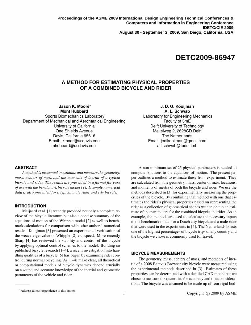
GeometryFifteen geometrical measurements (Fig. 1) of the bicycle

were taken using a ruler (±0.002 m) and an angle gage (±0.5deg). Only five of the measurements, w, c, λ 1, rR and rF, are re-quired for the benchmark model (Tab. 12). The rest of the mea-surements are used to estimate the seated position of the riderdescribed in the HUMAN PARAMETER ESTIMATION section.We use the same global coordinate system as the benchmarkmodel. The origin is at the rear wheel contact point with theX-axis pointing forward along the ground, the Z-axis downwardand the Y -axis to the right (Fig. 1). All of the dimensions weretaken as if they were projections into the XZ-plane except for thehub widths2. Note that in the model the top tube is assumed tobe horizontal and the measurements were taken from the inter-sections of tube centerlines. The wheel radii were measured byrolling the bicycle forward with the rider seated on the bicycle fornine revolutions of the wheel. The distance traversed along theground was measured with a ruler, divided by nine and convertedto wheel radii using the relationship between radius and circum-ference, r = c

2π. The head tube angle λht and the seat tube angle

λst were measured using an electronic angle gage while the bicy-cle was fixed in the upright position. The trail c was measured byaligning a straightedge along the centerline of the steering axisand measuring the distance along the ground between the frontwheel contact point and the end of the straight edge. The val-ues from the measurements of the Batavus Browser are shown inTab. 1.

MassThe bicycle was then disassembled into four parts represent-

ing four rigid bodies (rear wheel, front wheel, rear frame, andthe handlebar/fork assembly) to facilitate the measurement of theproperties of each individual body. The parts’ masses (Tab. 2)were measured using a large tabletop scale with an accuracy of±0.02 kg.

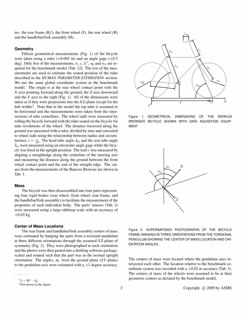
Center of Mass LocationsThe rear frame and handlebar/fork assembly centers of mass

were estimated by hanging the parts from a torsional pendulumat three different orientations through the assumed XZ-plane ofsymmetry (Fig. 2). They were photographed at each orientationand the photos were then pasted into a drafting software package,scaled and rotated such that the part was in the normal uprightorientation. The angles, αi, from the ground plane (XY -plane)to the pendulum axis were estimated with a ±1 degree accuracy.

1λ = 90◦−λht2Not shown in the figure.

Figure 1. GEOMETRICAL DIMENSIONS OF THE BATAVUSBROWSER BICYCLE SHOWN WITH DATA AQUISITION EQUIP-MENT.

Figure 2. SUPERIMPOSED PHOTOGRAPHS OF THE BICYCLEFRAME HANGING IN THREE ORIENTATIONS FROM THE TORSIONALPENDULUM SHOWING THE CENTER OF MASS LOCATION AND ORI-ENTATION ANGLES.

The centers of mass were located where the pendulum axes in-tersected each other. The location relative to the benchmark co-ordinate system was recorded with a ±0.02 m accuracy (Tab. 3).The centers of mass of the wheels were assumed to be at theirgeometric centers as dictated by the benchmark model.

2 Copyright c© 2009 by ASME

Table 1. BATAVUS BROWSER BICYCLE DIMENSIONS (ACCURACYOF±0.002 M AND±0.5 DEG).

Description Symbol Value Units

bottom bracket height hbb 0.295 m

chain stay length lcs 0.460 m

fork length l f 0.455 m

front hub width w f h 0.100 m

front wheel radius rF 0.342 m

handlebar length lhb 0.190 m

head tube angle λht 68.5 deg

rear hub width wrh 0.130 m

rear wheel radius rR 0.342 m

seat post length lsp 0.240 m

seat tube angle λst 68.5 deg

seat tube length lst 0.530 m

stem length ls 0.250 m

trail c 0.055 m

wheel base w 1.120 m

Table 2. BATAVUS BROWSER BICYCLE MASSES (ACCURACY OF±0.02 KG).

Description Symbol Value Units

front wheel mass mF 2.02 kg

handlebar/fork mass mH 4.35 kg

rear frame mass mB f 14.05 kg

rear wheel mass mR 3.12 kg

Moments of InertiaThree measurements were made to estimate the globally ref-

erenced moments and products of inertia (Ixx, Ixz and Izz) of therear frame and handlebar/fork assembly . The same torsionalpendulum used in [3] was used to measure the averaged periodT i of oscillation of the rear frame and handlebar/fork assembly atthree different orientation angles αi, where i = 1, 2, 3, as shownin Fig. 2. The parts were perturbed lightly, less than 1 degree,and allowed to oscillate about the pendulum axis through at leastten periods. The time of oscillation was recorded via a stop-

Table 3. POSITION OF THE CENTERS OF MASS OF THEREAR FRAME AND HANDLEBAR/FORK ASSEMBLY (ACCURACY OF±0.02 M).

Description Symbol Value Units

handlebar/fork (xH, zH) (0.88, -0.78) (m, m)

rear frame (xB f , zB f ) (0.25, -0.62) (m, m)

Table 4. REAR FRAME AND HANDLEBAR/FORK MEASURED MO-MENTS OF INERTIA.

Rear frame

i T i (s) αi (deg) Ji (kg m2)

1 3.60±0.06 41±1 1.65±0.05

2 3.40±0.06 81±1 1.47±0.05

3 2.50±0.06 150±1 0.79±0.04

Handlebar/fork assembly

i T i (s) αi (deg) Ji (kg m2)

1 1.50±0.06 37±1 0.29±0.02

2 0.70±0.03 105±1 0.06±0.01

3 1.20±0.06 139±1 0.18±0.02

watch (±1 s). This was done three times for each frame and therecorded times were averaged. The coefficient of elasticity k forthe torsional pendulum had previously been measured in [3] andfound to be k = 5.01± 0.01 Nm

rad . Three moments of inertia Jiabout the pendulum axes were calculated with

Ji =kT 2

i

4π2 (1)

and the numerical values are shown in Tab. 4.The moments and products of inertia of the rear frame and

handlebar/fork assembly with reference to the benchmark coor-dinate system were calculated by formulating the relationship be-tween inertial frames

Ji = RTi IRi (2)

where Ji is the inertia tensor about the pendulum axes, I, is theinertia tensor in the global reference frame and R is the rotation

3 Copyright c© 2009 by ASME

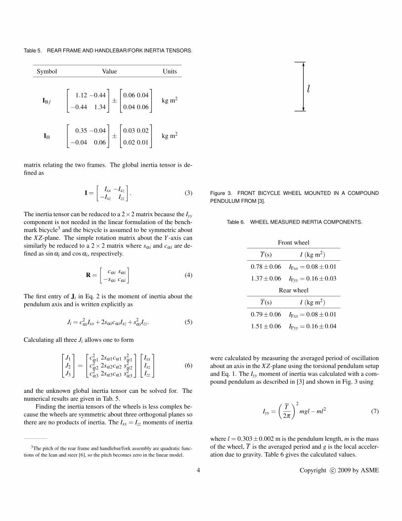
Table 5. REAR FRAME AND HANDLEBAR/FORK INERTIA TENSORS.

Symbol Value Units

IB f

1.12 −0.44

−0.44 1.34

±0.06 0.04

0.04 0.06

kg m2

IH

0.35 −0.04

−0.04 0.06

±0.03 0.02

0.02 0.01

kg m2

matrix relating the two frames. The global inertia tensor is de-fined as

I =[

Ixx −Ixz−Ixz Izz

]. (3)

The inertia tensor can be reduced to a 2×2 matrix because the Iyycomponent is not needed in the linear formulation of the bench-mark bicycle3 and the bicycle is assumed to be symmetric aboutthe XZ-plane. The simple rotation matrix about the Y -axis cansimilarly be reduced to a 2×2 matrix where sαi and cαi are de-fined as sinαi and cosαi, respectively.

R =[

cαi sαi−sαi cαi

](4)

The first entry of Ji in Eq. 2 is the moment of inertia about thependulum axis and is written explicitly as

Ji = c2αiIxx +2sαicαiIxz + s2

αiIzz. (5)

Calculating all three Ji allows one to form

J1J2J3

=

c2α1 2sα1cα1 s2

α1c2

α2 2sα2cα2 s2α2

c2α3 2sα3cα3 s2

α3

IxxIxzIzz

(6)

and the unknown global inertia tensor can be solved for. Thenumerical results are given in Tab. 5.

Finding the inertia tensors of the wheels is less complex be-cause the wheels are symmetric about three orthogonal planes sothere are no products of inertia. The Ixx = Izz moments of inertia

3The pitch of the rear frame and handlebar/fork assembly are quadratic func-tions of the lean and steer [6], so the pitch becomes zero in the linear model.

Figure 3. FRONT BICYCLE WHEEL MOUNTED IN A COMPOUNDPENDULUM FROM [3].

Table 6. WHEEL MEASURED INERTIA COMPONENTS.

Front wheel

T (s) I (kg m2)

0.78±0.06 IFxx = 0.08±0.01

1.37±0.06 IFyy = 0.16±0.03

Rear wheel

T (s) I (kg m2)

0.79±0.06 IFxx = 0.08±0.01

1.51±0.06 IFyy = 0.16±0.04

were calculated by measuring the averaged period of oscillationabout an axis in the XZ-plane using the torsional pendulum setupand Eq. 1. The Iyy moment of inertia was calculated with a com-pound pendulum as described in [3] and shown in Fig. 3 using

Iyy =(

T2π

)2

mgl−ml2 (7)

where l = 0.303±0.002 m is the pendulum length, m is the massof the wheel, T is the averaged period and g is the local acceler-ation due to gravity. Table 6 gives the calculated values.

4 Copyright c© 2009 by ASME

HUMAN PARAMETER ESTIMATIONThe measurement of the physical properties of a human is

more difficult than for a bicycle because the human body partsare not as easily described as rigid bodes with defined joints andinflexible geometry. Dohring [7] measured the moments of in-ertia and centers of mass of a combined rider and motor-scooterwith a large measurement table, but this is not always practical.The validity of the present method could be determined if suchdata existed for a bicycle and rider.

Many methods exist for estimating the geometry, centersof mass and moments of inertia of a human including ca-daver measurements [8–10], photogrammetry, ray scanning tech-niques [11, 12], water displacement [13], and mathematical geo-metrical estimation of the body segments [14]. We estimated thephysical properties of the rider in a seated position using a sim-ple mathematical geometrical estimation similar in idea to [14]in combination with mass data from [8].

Several measurements of the human rider were needed tocalculate the physical properties. The mass of the rider was mea-sured along with fourteen anthropomorphic measurements of thebody (Tab. 7 and Tab. 8). These measurements in combinationwith the geometrical bicycle measurements taken in the previ-ous section (Tab. 1) are used to define a model of the rider madeup of simple geometrical shapes (Fig. 4). The legs and arms arerepresented by cylinders, the torso by a cuboid and the head by asphere. The feet are positioned at the center of the pedaling axisto maintain symmetry about the XZ-plane.

All but one of the anthropomorphic measurements weretaken when the rider was standing casually on flat ground. Thelower leg length lll is the distance from the floor to the knee joint.The upper leg length lul is the distance from the knee joint to thehip joint. The length from hip to hip lhh and shoulder to shoulderlss are the distances between the two hip joints and two shoulderjoints, respectively. The torso length lto is the distance betweenhip joints and shoulder joints. The upper arm length lua is thedistance between the shoulder and elbow joints. The lower armlength lal is the distance from the elbow joint to the center of thehand when the arm is outstretched. The circumferences are takenat the cross section of maximum circumference (e.g. around thebicep, around the brow, over the nipples for the chest). The for-ward lean angle λ f l is the approximate angle made between thefloor (XY -plane) and the line connecting the center of the rider’shead and the top of the seat while the rider is seated normallyon the bicycle. This was estimated by taking a side profile pho-tograph of the rider on the bicycle and scribing a line from thehead to the top of the seat. The measurements were made as ac-curately as possible with basic tools but no special attention isgiven further to the accuracy of the calculations due to the factthat modeling the human as basic geometric shapes already intro-duces a large error. The values are reported to the same decimalplaces as the previous section for consistency.

The masses of each segment (Tab. 8) were defined as a pro-

Table 7. RIDER ANTRHOPOMORPHIC MEASUREMENTS.

Description Symbol Value Units

chest circumference cch 0.94 m

forward lean angle λ f l 82.9 deg

head circumference ch 0.58 m

hip joint to hip joint lhh 0.26 m

lower arm circumference cla 0.23 m

lower arm length lla 0.33 m

lower leg circumference cc 0.38 m

lower leg length lll 0.46 m

shoulder to shoulder lss 0.44 m

torso length lto 0.48 m

upper arm circumference cua 0.30 m

upper arm length lua 0.28 m

upper leg circumference cul 0.50 m

upper leg length lul 0.46 m

Table 8. BODY MASS AND SEGMENT MASSES.

Segment Symbol Equation Value Unit

mass of rider body mBr N/A 72.0 kg

head mh 0.068mBr 4.90 kg

lower arm mla 0.022mBr 1.58 kg

lower leg mll 0.061mBr 4.39 kg

torso mto 0.510mBr 36.72 kg

upper arm mua 0.028mBr 2.02 kg

upper leg mul 0.100mBr 7.20 kg

portion of the total mass of the rider mBr using data from cadaverstudies by [8].

The geometrical and anthropomorphic measurements wereconverted into a set of 31 grid points in three dimensional spacethat mapped the skeleton of the rider and bicycle (Fig. 4). Theposition vectors to these grid points are listed in Tab. 10. Severalintermediate variables used in the grid point equations are listedin Tab. 11 where fo is the fork offset and the rest arise from themultiple solutions to the location of the elbow and knee jointsand have to be solved for using numeric methods. The correct

5 Copyright c© 2009 by ASME

1

6

8

11

4

526 27

28 29

12

17 19

23

21

25

15

22

24

3130

13

10

9

3

16

18 20

7

2

14

Figure 4. LOCATIONS OF GRID POINTS AND SIMPLE GEOMETRICSHAPES. SEE ALSO TAB. 10.

solutions are the ones that force the arms and legs to bend in anatural fashion. The grid points mark the center of the sphereand the end points of the cylinders and cuboid. The segments arealigned along lines connecting the appropriate grid points. Thesegments are assumed to have uniform density so the centers ofmass are taken to be at the geometrical centers. The midpointformula is used to calculate the local centers of mass for eachsegment in the global reference frame. The total body center ofmass can be found from the standard formula

rBr = ∑miri

mBr= [0.291 0 −1.109]m (8)

where ri is the position vector to the centroid of each segmentand mi is the mass of each segment. The local moments of iner-tia of each segment are determined using the ideal definitions ofinertia for each segment type (Tab. 9). The width of the cuboidrepresenting the torso ly is defined by the shoulder width and up-per arm circumference.

ly = lss−cua

π(9)

The cuboid thickness was estimated using the chest circumfer-

Table 9. SEGMENT INTERIA TENSORS. HERE THE x, y AND z AXESARE LOCAL.

Segment Moment of Inertia

cuboid 112 m

l2y + l2

z 0 0

0 l2x + l2

z 0

0 0 l2x + l2

y

cylinder Ix, Iy = 1

12 m(

3c2

4π2 + l2)

, Iz = mc2

8π2

sphere Ix, Iy, Iz = mc2

10π2

ence measurement and assuming that the cross section of thechest is similar to a stadium shape.

lx =cch−2ly

π−2(10)

The local zi unit vector for the segments was defined alongthe line connecting the associated grid points from the lowernumbered grid point to the higher numbered grid point. The lo-cal unit vector in the y direction was set equal to the global Yunit vector with the xi unit vector following from the right handrule. The rotation matrix needed to rotate each of the moments ofinertia to the global reference frame can be calculated by dottingthe global unit vectors X, Y, Z with the local unit vectors xi, yi,zi for each segment.

Ri =

X · xi X · yi X · ziY · xi Y · yi Y · ziZ · xi Z · yi Z · zi

(11)

The local inertia matrices are then rotated to the global referenceframe with

Ii = RiJiRTi . (12)

The local moments of inertia can then be translated to the centerof mass of the entire body using the parallel axis theorem

I∗i = Ii +mi

d2y +d2

z −dxdy −dxdz

−dxdy d2z +d2

x −dydz−dxdz −dydz d2

x +d2y

(13)

where dx, dy and dz are the distances along the the X , Y and Zaxes, respectively, from the local center of mass to the global

6 Copyright c© 2009 by ASME

center of mass. Finally, the local translated and rotated momentsof inertia are summed to give the total moment of inertia of therider by

IBr = ∑I∗i =

8.00 0 −1.930 8.07 0

−1.93 0 2.36

kg m2. (14)

COMBINED REAR FRAME AND RIDERThe mass, center of mass and moment of inertia is calculated

similarly to what was previously described. The total mass is

mB = mB f +mBr. (15)

The center of mass position is

rB =mB f rB f +mBrrBr

mB. (16)

The two moments of inertia are translated to the center of masslocation using the parallel axis theorem (Eq. 13) and the compo-nents summed to find the final moments of inertia.

RESULTSThe final results are presented in the form used by the bench-

mark model (Tab. 12). These can be used to populate the canon-ical form

Mq+ vC1q+[gK0 + v2K2

]q = 0 (17)

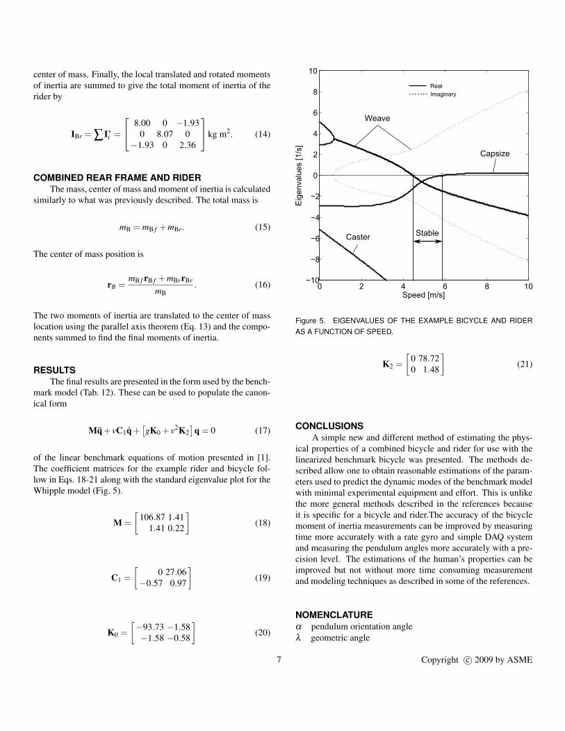
of the linear benchmark equations of motion presented in [1].The coefficient matrices for the example rider and bicycle fol-low in Eqs. 18-21 along with the standard eigenvalue plot for theWhipple model (Fig. 5).

M =[

106.87 1.411.41 0.22

](18)

C1 =[

0 27.06−0.57 0.97

](19)

K0 =[−93.73 −1.58−1.58 −0.58

](20)

0 2 4 6 8 10−10

−8

−6

−4

−2

0

2

4

6

8

10

Speed [m/s]E

igen

valu

es [1

/s]

Weave

Capsize

Caster

RealImaginary

Stable

Figure 5. EIGENVALUES OF THE EXAMPLE BICYCLE AND RIDERAS A FUNCTION OF SPEED.

K2 =[

0 78.720 1.48

](21)

CONCLUSIONSA simple new and different method of estimating the phys-

ical properties of a combined bicycle and rider for use with thelinearized benchmark bicycle was presented. The methods de-scribed allow one to obtain reasonable estimations of the param-eters used to predict the dynamic modes of the benchmark modelwith minimal experimental equipment and effort. This is unlikethe more general methods described in the references becauseit is specific for a bicycle and rider.The accuracy of the bicyclemoment of inertia measurements can be improved by measuringtime more accurately with a rate gyro and simple DAQ systemand measuring the pendulum angles more accurately with a pre-cision level. The estimations of the human’s properties can beimproved but not without more time consuming measurementand modeling techniques as described in some of the references.

NOMENCLATUREα pendulum orientation angleλ geometric angle

7 Copyright c© 2009 by ASME

c circumference except for the definition of trail that matchesthe benchmark model from [1] and the abbreviation for cos

cα cosα

d distancefo fork offsetg local acceleration due to gravityh heightk pendulum torsional stiffnessl lengthm massr radiuss, t, u, v intermediate variables, v is also used for forward speedsα sinα

w width except for the definition of wheelbase that matches thebenchmark model

x center of mass x coordinate for the benchmark bicyclez center of mass z coordinate for the benchmark bicycleI global inertia componentJ inertia componentT periodq state vectorr position vector defined relative to the benchmark reference

frame [rX rY rZ ] or to a local reference frame [rx ry rz]xyz local axesR rotation matrixI globally referenced inertia matrixJ inertia matrixM, C1, K0, K2 benchmark canonical matricesXYZ global axes

REFERENCES[1] Meijaard, J. P., Papadopoulos, J. M., Ruina, A., and

Schwab, A. L., 2007. “Linearized dynamics equations forthe balance and steer of a bicycle: A benchmark and re-view”. Royal Society of London Proceedings Series A, 463,August, pp. 1955–1982.

[2] Whipple, F. J. W., 1899. “The stability of the motion of abicycle”. Quarterly Journal of Pure and Applied Mathe-matics, 30, pp. 312–348.

[3] Kooijman, J. D. G., 2006. “Experimental validation of amodel for the motion of an uncontrolled bicycle”. MScthesis, Delft University of Technology.

[4] Sharp, R. S., 2008. “On the stability and control of thebicycle”. Applied Mechanics Reviews, 61(6), November,p. 24.

[5] Kooijman, J. D. G., and Schwab, A. L., 2008. “Some obser-vations on human control of a bicycle”. In 11th mini Con-ference on Vehicle System Dynamics, Identification andAnomalies (VSDIA2008), Budapest, Hungary, I. Zobory,ed., Budapest University of Technology and Economincs,p. 8.

[6] Petersen, D. L., and Hubbard, M., 2007. “Analysis of theholonomic constraint in the Whipple bicycle model”. InThe Engineering of Sport: 7, M. Estivalet and P. Brisson,eds., Springe.

[7] Dohring, E., 1953. “Uber die stabilitat und die lenkkraftevon einspurfahrzeugen”. PhD thesis, Technical UniversityBraunschweig, Germany.

[8] Dempster, W. T., 1955. Space requirements of the seatedoperator, geometrical, kinematic and mechanical aspects ofthe body with special reference to the limbs. Technical Re-port WADC 55-159, Wright-Patterson AFB, Ohio.

[9] Clauser, C. E., McConville, J. T., and Young, J. W., 1969.Weight, volume and center of mass of segments of the hu-man body. Tech. Rep. AMRL TR 69-70, Wright-PattersonAir Force Base, Ohio. NTIS No. AD-710 622.

[10] Chandler, R. F., Clauser, C. E., McConville, J. T., Reynolds,H. M., and Young, J. W., 1975. Investigation of inertialproperties of the human body. Tech. Rep. AMRL TR 74-137, Wright-Patterson Air Force Base, Ohio. NTIS No.AD-A016 485.

[11] Zatsiorsky, V., and Seluyanov, V., 1983. “The mass andinertia characteristics of the main segments of the hu-man body”. In Biomechanics VIII-B, H. Matsui andK. Kobayashi, eds., Human Kinetic, pp. 1152–l 159.

[12] Zatsiorsky, V., Seluyanov, V., and Chugunova, L., 1990.“In vivo body segment inertial parameters determinationusing a gamma-scanner method”. In Biomechanics of Hu-man Movement: Applications in Rehabilitation, Sports andErgonomics, N. Berme and A. Cappozzo, eds., Bertec,pp. 186–202.

[13] Park, S. J., Kim, C., and Park, S. C., 1999. “Anthropomet-ric and biomechanical characteristics on body segments ofKoreans”. Applied Human Sciences, 18(3), May, pp. 91–9.

[14] Yeadon, M. R., 1990. “The simulation of aerial movement-II. A mathematical inertia model of the human body”. Jour-nal of Biomechanics, 23, pp. 67–74.

8 Copyright c© 2009 by ASME

Table 10. SKELETON GRID POINTS WITH RESPECT TO THE GLOBAL FRAME. SEE FIG. 4

Description Equation Value (m)

rear contact point r1 = [0 0 0] [0 0 0]

rear wheel center r2 = [0 0 − rR] [0 0 −0.342]

right rear hub center r3 = r2 +[0 wrh

2 0]

[0 0.065 −0.342]

left rear hub center r4 = r2 +[0 − wrh

2 0]

[0 −0.065 −0.342]

bottom bracket center r5 =[√

l2cs− (rR−hbb)2 0 −hbb

][0.458 0 −0.295]

front wheel contact point r6 = [w 0 0] [1.120 0 0]

front wheel center r7 = r6 +[0 0 − rF] [1.120 0 −0.342]

right front hub center r8 = r7 +[0 w f h

2 0]

[1.120 0.050 −0.342]

left front hub center r9 = r7 +[0 − w f h

2 0]

[1.120 −0.050 −0.342]

left front hub center r10 = r5 +[−lst cosλst 0 − lst sinλst ] [0.263 0 −0.788]

top of seat tube r11 = r7 +[− fo sinλht − cosλht

√l2

f − f 2o 0 fo cosλht − sinλht

√l2

f − f 2o

][0.887 0 −0.733]

top of head tube r12 =[rX11− rZ11−rZ10

tanλht0 rZ10

][0.865 0 −0.788]

top of seat r13 = r10 +[−lsp cosλst 0 − lsp sinλst

][0.175 0 −1.011]

center of knees r14 = r5 +[s 0 − t] [0.551 0 −0.746]

shoulder midpoint r15 = r13 +[lto cosλ f l 0 − lto sinλ f l

][0.235 0 −1.488]

top of stem r16 = r12 +[−ls cosλht 0 − ls sinλht ] [0.773 0 −1.021]

right handlebar r17 = r16 +[0 lss

2 0]

[0.773 0.220 −1.021]

left handlebar r18 = r16 +[0 − lss

2 0]

[0.773 −0.220 −1.021]

right hand r19 = r17 +[−lhb 0 0] [0.583 0.220 −1.021]

left hand r20 = r18 +[−lhb 0 0] [0.583 −0.220 −1.021]

right shoulder r21 = r15 +[0 lss

2 0]

[0.235 0.220 −1.488]

left shoulder r22 = r15 +[0 − lss

2 0]

[0.235 −0.220 −1.488]

right elbow r23 = r19 +[−u lss

2 − v]

[0.321 0.220 −1.222]

left elbow r24 = r23 +[0 − lss 0] [0.321 −0.220 −1.222]

center of head r25 = r15 +[ ch

2πcosλ f l 0 − ch

2πsinλ f l

][0.246 0 −1.579]

right foot r26 = r5 +[0 lhh

2 0]

[0.458 0.130 −0.295]

left foot r27 = r5 +[0 − lhh

2 0]

[0.458 −0.130 −0.295]

right knee r28 = r14 +[0 lhh

2 0]

[0.551 0.130 −0.746]

left knee r29 = r14 +[0 − lhh

2 0]

[0.551 −0.130 −0.746]

right hip r30 = r13 +[0 lhh

2 0]

[0.175 0.130 −1.011]

left hip r31 = r13 +[0 − lhh

2 0]

[0.175 −0.130 −1.011]

9 Copyright c© 2009 by ASME

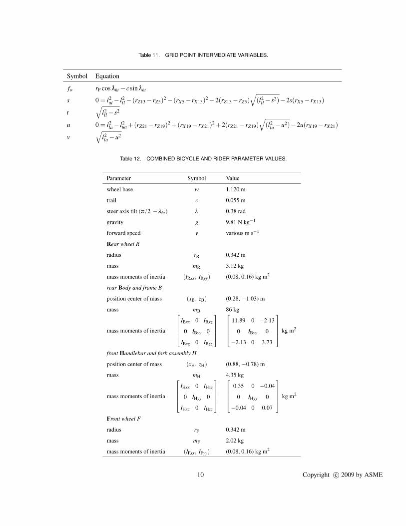
Table 11. GRID POINT INTERMEDIATE VARIABLES.

Symbol Equation

fo rF cosλht − csinλht

s 0 = l2ul − l2

ll − (rZ13− rZ5)2− (rX5− rX13)2−2(rZ13− rZ5)√

(l2ll − s2)−2s(rX5− rX13)

t√

l2ll − s2

u 0 = l2la− l2

ua +(rZ21− rZ19)2 +(rX19− rX21)2 +2(rZ21− rZ19)√

(l2la−u2)−2u(rX19− rX21)

v√

l2la−u2

Table 12. COMBINED BICYCLE AND RIDER PARAMETER VALUES.

Parameter Symbol Value

wheel base w 1.120 m

trail c 0.055 m

steer axis tilt (π/2 −λht ) λ 0.38 rad

gravity g 9.81 N kg−1

forward speed v various m s−1

Rear wheel R

radius rR 0.342 m

mass mR 3.12 kg

mass moments of inertia (IRxx, IRyy) (0.08, 0.16) kg m2

rear Body and frame B

position center of mass (xB, zB) (0.28, −1.03) m

mass mB 86 kg

mass moments of inertia

IBxx 0 IBxz

0 IByy 0

IBxz 0 IBzz

11.89 0 −2.13

0 IByy 0

−2.13 0 3.73

kg m2

front Handlebar and fork assembly H

position center of mass (xH, zH) (0.88, −0.78) m

mass mH 4.35 kg

mass moments of inertia

IHxx 0 IHxz

0 IHyy 0

IHxz 0 IHzz

0.35 0 −0.04

0 IHyy 0

−0.04 0 0.07

kg m2

Front wheel F

radius rF 0.342 m

mass mF 2.02 kg

mass moments of inertia (IFxx, IFyy) (0.08, 0.16) kg m2

10 Copyright c© 2009 by ASME