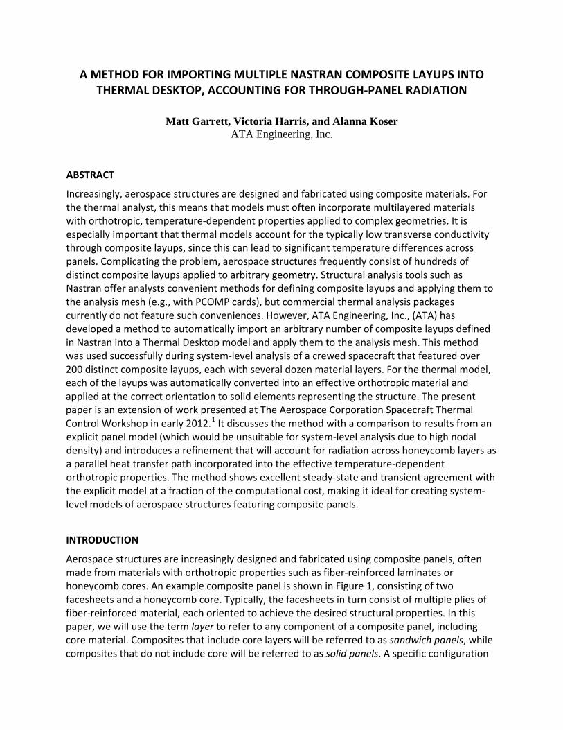
A METHOD FOR IMPORTING MULTIPLE NASTRAN COMPOSITE LAYUPS INTO THERMAL DESKTOP, ACCOUNTING FOR THROUGH‐PANEL RADIATION 

Matt Garrett, Victoria Harris, and Alanna Koser ATA Engineering, Inc.

ABSTRACT 

Increasingly, aerospace structures are designed and fabricated using composite materials. For the thermal analyst, this means that models must often incorporate multilayered materials with orthotropic, temperature‐dependent properties applied to complex geometries. It is especially important that thermal models account for the typically low transverse conductivity through composite layups, since this can lead to significant temperature differences across panels. Complicating the problem, aerospace structures frequently consist of hundreds of distinct composite layups applied to arbitrary geometry. Structural analysis tools such as Nastran offer analysts convenient methods for defining composite layups and applying them to the analysis mesh (e.g., with PCOMP cards), but commercial thermal analysis packages currently do not feature such conveniences. However, ATA Engineering, Inc., (ATA) has developed a method to automatically import an arbitrary number of composite layups defined in Nastran into a Thermal Desktop model and apply them to the analysis mesh. This method was used successfully during system‐level analysis of a crewed spacecraft that featured over 200 distinct composite layups, each with several dozen material layers. For the thermal model, each of the layups was automatically converted into an effective orthotropic material and applied at the correct orientation to solid elements representing the structure. The present paper is an extension of work presented at The Aerospace Corporation Spacecraft Thermal Control Workshop in early 2012.1 It discusses the method with a comparison to results from an explicit panel model (which would be unsuitable for system‐level analysis due to high nodal density) and introduces a refinement that will account for radiation across honeycomb layers as a parallel heat transfer path incorporated into the effective temperature‐dependent orthotropic properties. The method shows excellent steady‐state and transient agreement with the explicit model at a fraction of the computational cost, making it ideal for creating system‐level models of aerospace structures featuring composite panels. 

INTRODUCTION 

Aerospace structures are increasingly designed and fabricated using composite panels, often made from materials with orthotropic properties such as fiber‐reinforced laminates or honeycomb cores. An example composite panel is shown in Figure 1, consisting of two facesheets and a honeycomb core. Typically, the facesheets in turn consist of multiple plies of fiber‐reinforced material, each oriented to achieve the desired structural properties. In this paper, we will use the term layer to refer to any component of a composite panel, including core material. Composites that include core layers will be referred to as sandwich panels, while composites that do not include core will be referred to as solid panels. A specific configuration 

of layers will be called a layup. A panel‐based coordinate system will be employed, with the xy‐plane aligned with the panel and the z‐axis normal to it. 

 

Figure 1. Example composite sandwich panel with honeycomb core.1 

Systems constructed of composite panels present several challenges to the thermal analyst. One challenge is the low allowable temperature for many composite materials. For example, on a very hot day, the maximum allowable temperature for composite aircraft nacelles may be just 20 K above the temperature of the cooling air available aft of the engine fan. For this reason, analysis of composite assemblies must be precise. Complicating matters, ply materials—and thus whole panels—often have low out‐of‐plane (OOP) thermal conductivity, which leads to significant through‐panel temperature gradients. Therefore, the thermal analyst must model through‐panel conduction; i.e., the analyst cannot treat composite panels as simple isothermal shells. However, any analysis method that relies on explicit panel geometry to model through‐panel conduction will meet with failure for two reasons: composite aerospace systems consist of dozens or hundreds of layups, and the layups are oriented and connected arbitrarily. Managing the explicit geometry for so many layups would not be feasible, and transitioning between layups would likely lead to hanging nodes and other connectivity issues. See Figure 2 for an example model of a composite system containing hundreds of layups. A final challenge for the thermal analyst is that composite material properties are often temperature dependent over the temperature ranges of interest. While this is not difficult to accommodate, it must be considered. 

 

  TFAWS 2012 – August 13‐17, 2012  2  

 

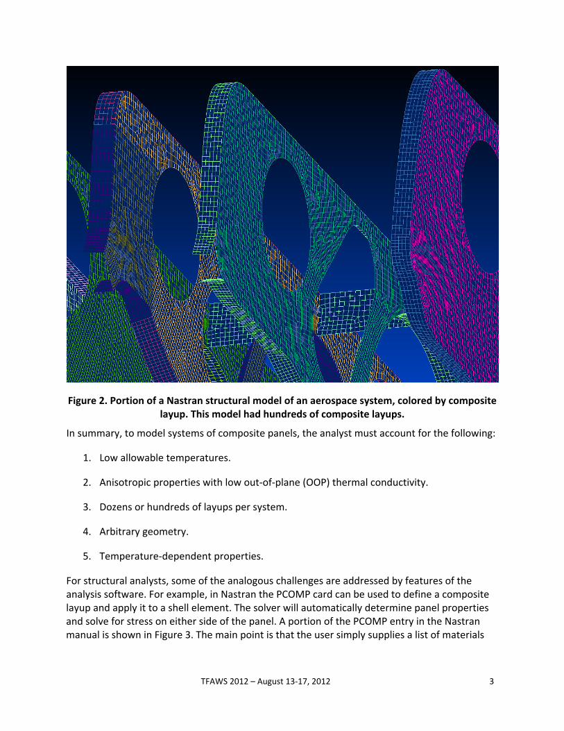
Figure 2. Portion of a Nastran structural model of an aerospace system, colored by composite layup. This model had hundreds of composite layups. 

In summary, to model systems of composite panels, the analyst must account for the following: 

1. Low allowable temperatures. 

2. Anisotropic properties with low out‐of‐plane (OOP) thermal conductivity. 

3. Dozens or hundreds of layups per system. 

4. Arbitrary geometry. 

5. Temperature‐dependent properties. 

For structural analysts, some of the analogous challenges are addressed by features of the analysis software. For example, in Nastran the PCOMP card can be used to define a composite layup and apply it to a shell element. The solver will automatically determine panel properties and solve for stress on either side of the panel. A portion of the PCOMP entry in the Nastran manual is shown in Figure 3. The main point is that the user simply supplies a list of materials 

 

  TFAWS 2012 – August 13‐17, 2012  3  

(MID1, 2, etc., in the manual), thicknesses (T1, 2, etc.), and orientation angles (THETA1, 2, etc.) to define a composite layup in a Nastran model. Once defined, the layup can be applied to elements by referring to the property ID, listed as PID in the manual. 

 

Figure 3. Portion of the PCOMP entry in the Nastran manual.3 

The layup defined by a PCOMP card may have different properties in the x and y in‐plane directions. Fortunately, modern Nastran preprocessors give the user several advanced tools for specifying the material coordinate system of each element (see Figure 4). 

 

Figure 4. Nastran model created using Siemens NX.4 A single command oriented the material coordinate systems (x‐axes shown as arrows) of all of the elements, despite the considerable 

curvature of the system. 

Since the MIDs refer to material cards that can store anisotropic, temperature‐dependent properties, the combination of PCOMPs, material cards, and advanced tools for orienting material coordinate systems addresses all but the first challenge listed above; for the structural analyst, the analysis software provides adequate tools to aid in the massive amount of bookkeeping required to model systems of composite panels. 

The thermal analyst is not so fortunate. Here we will discuss these issues with regard to Cullimore and Ring Technologies’ Thermal Desktop (T‐D)5 due to its popularity among aerospace thermal analysts. T‐D is a powerful general‐purpose thermal analysis package. However, it does not currently offer the thermal analyst the same conveniences the structural analyst enjoys with regard to modeling composite structures. There are three reasons for this: 

 

  TFAWS 2012 – August 13‐17, 2012  4  

 

  TFAWS 2012 – August 13‐17, 2012  5  

1. There is no equivalent to the Nastran PCOMP card in T‐D; i.e., the thermal analyst cannot define a composite layup simply by providing the software with a list of materials, thicknesses, and orientations. The Stack Manager is a step in this direction, but it currently only applies to 1‐D insulation networks. 

2. Finite Element (FE) shell elements cannot model OOP conduction, since they cannot support through‐panel temperature differences. Finite Difference (FD) shells can model OOP conduction but are unsuitable for the complex, arbitrary geometries thermal analysts are expected to model with fidelity, since the FD shell creation tools are meant for approximating complex geometries as simple shapes. 

3. Material orientation definition is limited. Within T‐D, the user creates and manipulates material orienters manually and then applies them to elements. We are unaware of a technique for creating multiple material orienters aligned with elemental coordinate systems and associated to their respective elements. This is a common feature in Nastran preprocessors, which we used to create material coordinate systems for the structural model shown in Figure 4. 

This paper discusses a method we developed to overcome these limitations by semi‐automatically importing an arbitrary number of composite layups with orthotropic, temperature‐dependent properties into T‐D and applying them at the correct orientations to a thermal finite element model (FEM). 

PROBLEM 

As discussed above, Nastran and its preprocessors have features that allow the structural analyst to define layups as stacks of orthotropic materials with temperature‐dependent properties and then apply those layups to shell elements with easily manipulated material orientations. We set out to provide similar functionality to the thermal analyst using T‐D, making use of Nastran and Nastran preprocessors wherever possible since they are already optimized for working with composites. The problem can be stated as follows: 

Given a Nastran shell model with composite panels, semi‐automatically import the model into T‐D while accounting for through‐panel temperature differences, orthotropic and temperature‐dependent material properties, radiation across core layers, and material orientation on the mesh. 

METHOD OVERVIEW 

In this section, each step will be highlighted and followed by an explanation of why it was included in the method, along with some tips on how to implement it. 

Step A. (Optional) Reduce the node count of the structural mesh. 

 

  TFAWS 2012 – August 13‐17, 2012  6  

Since structural meshes are frequently much finer than thermal meshes, we use Nastran preprocessors to reduce the node count while maintaining the geometric shape of the mesh and any important node lines, e.g., transitions between panel layups, thermal protection system (TPS) layups, boundary conditions, etc. If the mesh is associated with geometry, we use Siemens NX. If no geometry is available, we use Altair Hypermesh,6 which features powerful tools for manipulating meshes absent of geometry. Details of their use are outside the scope of this paper. 

Step B. Convert the Nastran shell mesh into a Nastran thin solid mesh. 

We determined that any method that meshed each layer of each layup would fail, since the node count would be ridiculously high for a system‐level model with layups of dozens of layers. Meshing the transitions between layups would also be problematic, as different layups would require different numbers of through‐thickness nodes. These issues are not a concern for structural analysts, since shell elements can adequately model composite panels for structural analysis. 

As a compromise, we used thin solid elements with effective orthotropic properties in T‐D to describe each layup. To deal with the transitions between layups, we modeled all panels using a standard dummy thickness and then scaled all properties to account for the actual panel thickness via property multipliers applied to each element.  

We chose this approach even though it does not allow a detailed temperature distribution across the panel to be calculated. Such a detailed temperature distribution is usually unimportant for a system‐level model; typically, only the extreme temperatures at the inner and outer faces are required. 

We found that Hypermesh was good for creating thin solid meshes from shell meshes while maintaining appropriate nodal connectivity at corners, T‐joints, etc. 

Step C. Assign a material to each PCOMP card, with the dummy material ID matching its corresponding PCOMP ID number. 

When the Nastran mesh is finally imported into T‐D, each element is assigned a T‐D material based on the material ID in the Nastran input deck. This step ensures that the T‐D material name matches the original PCOMP ID. 

 

  TFAWS 2012 – August 13‐17, 2012  7  

This is a simple change and can be performed using a text editor on the Nastran input deck. Of course, this step could also be automated with a script that acts on the input deck, or it could be performed within a Nastran preprocessor before creating the input deck, perhaps automatically. 

Step D. Create the Nastran input deck with explicit CORD2R coordinate systems defined for each element. 

It is important that materials are oriented correctly on each element. We worked with C&R to update the T‐D Nastran importer so that it would create a material orienter for each solid element in a Nastran deck, if the element is defined as in Figure 5.  

CHEXA 2108 1200193 227 348 368 67 2197 2201+ + 2205 2198 PSOLID 1200193 1200015 182 CORD2R 182 0 0.0 0.0 0.01.3300-31.3000-31.000000+ + -.026380-.9996501.3300-3

Figure 5. Nastran deck excerpt showing required solid element definition format. 

In this example, the CHEXA card defines solid element 2108. The second integer in the CHEXA card, 1200193, points to a PSOLID property card, which in turn identifies coordinate system 182 as the material coordinate system for this element. The specifics of the coordinate system are defined using the CORD2R card. As of T‐D version 5.4 Patch 7e, the Nastran importer understands this syntax and will create a material orienter and assign it to element 2108 in this example. See Reference 3 for more information about the format of Nastran input decks. 

This Nastran deck format is usually not the default in Nastran preprocessors, but it can be achieved by modifying the output options. We used Siemens I‐deas7 and selected the “Heat” approach when writing the Nastran deck. 

Step E. Import the thin solid mesh into T‐D. 

At the conclusion of this step, we have a thin solid mesh in T‐D. Each element is associated with a dummy material whose name is “M#,” where “#” is the original PCOMP ID associated with that element in the structural model. Each element also has a T‐D material orienter associated with it, aligned with the z‐axis normal to the panel and the x‐ and y‐axes aligned appropriately. 

Step F. Update each T‐D solid element with property multipliers that account for actual thickness. 

This step is required since the elements are modeled using a standard dummy thickness to aid in connectivity. By adjusting element‐level property multipliers to the specific dummy thickness used, the effective material definition remains a pure description of the layup unburdened by model‐specific property multipliers. 

 

  TFAWS 2012 – August 13‐17, 2012  8  

Step G. Create MAT5/MATT5 entries for each layer material. 

Since the original model was for structural analysis, it is unlikely that the layer materials referenced by the PCOMPs are described using Nastran cards that support thermal data. By creating MAT5/MATT5 entries for each layer material, orthotropic and temperature‐dependent thermal material properties are introduced into the model. The material ID of these entries should match the material ID of the corresponding structural material definition. 

Step H. Automatically convert each PCOMP into a Nastran MAT5/MATT5 orthotropic thermal material with temperature‐dependent properties. 

We developed a script that scans the structural Nastran input deck for PCOMP entries. For each entry, it creates an effective orthotropic material in Nastran MAT5/MATT5 format, using calculations discussed in the next section and the thermal layer materials discussed in Step G. We worked with C&R to update the T‐D Nastran importer; as of T‐D version 5.4 Patch 7j, it will create an orthotropic T‐D material for each MAT5/MATT5 entry in a Nastran deck. 

Step I. Import the effective materials representing each PCOMP layup into a blank T‐D model. 

This creates a T‐D orthotropic material for each MAT5/MATT5 entry in the Nastran deck containing the effective materials created in the previous step. If this is done in an empty T‐D model, these materials will have the same names as the materials created when the thin solid mesh was imported into T‐D, i.e., “M#,” where “#” is the original PCOMP ID from the solid model. If this is not done in an empty T‐D model, the importer may change the names of the newly imported materials to avoid duplicates, breaking the link between the effective materials and the original PCOMP IDs. 

Step J. Merge the T‐D thin solid mesh model and the T‐D model containing the effective thermal properties representing composite layups. 

This is accomplished simply by overwriting the thin solid model thermophysical database file with the one that contains the effective properties created in the previous step. 

METHOD DETAILS 

This section elaborates on the algorithm used in PCOMP2MAT5, the script developed to convert each Nastran PCOMP entry into an effective orthotropic material described using MAT5/MATT5 cards. This script was created using Mathworks’ MATLAB8 and ATA’s commercially available interface between MATLAB, analysis, and test, IMAT.9 IMAT provides tools for reading and writing Nastran input decks. 

PCOMP2MAT5 scans the input deck for PCOMP entries. For each PCOMP entry, it performs the following calculations: 

Step 1. Determine an appropriate temperature range for each material property. 

Each layup is composed of layers of materials defined in separate MAT5/MATT5 entries. In general, each property array referenced by each MATT5 entry has a distinct temperature range. The script examines those arrays and determines an appropriate temperature range for each property of each layup. Currently, it uses the smallest range that envelopes all layer temperature ranges and warns the user if the extreme temperatures deviate more than an allowable margin above or below any of the layer temperature ranges. 

When determining approximate property values at temperatures not listed in the layer property arrays, the script uses a linear interpolation between the nearest two data points, unless the temperature is above the high endpoint temperature or below the low endpoint temperature. In this case, rather than extrapolating, it assumes that the endpoint property values are constant at temperatures above and below the endpoints. 

Step 2. Transform the in‐plane conductivities of each layer into the layup x and y directions. 

PCOMP cards allow each layer to be oriented with respect to the layup coordinate system via the THETAx entry for each layer (see Figure 3). Often, layers such as core or fabric have the same conductivity in all planar directions, but for generality, the script transforms the layer in‐plane conductivities into the layup x and y directions using a thermal analog of the planar stress transformation equations with zero shear:10 

,  (1)

where kxx and kyy are the layer conductivities in the layup x and y directions, kmx and kmy are the layer conductivities in the layer x and y directions (from the MAT5/MATT5 entry for the layer), and θ is the orientation angle of the layer with respect to the layup (obtained from the layup PCOMP entry). These calculations are performed for several temperatures across the temperature range determined in step A. 

Step 3. Calculate the effective overall in‐plane conductivities in the x and y directions for each layup. 

The script combines the in‐plane conductivities for each layer calculated in the previous step as thickness‐weighted average effective x and y layup conductivities at several temperatures across the appropriate range determined in step A. 

 

  TFAWS 2012 – August 13‐17, 2012  9  

 A thickness‐weighted average conductivity is equivalent to calculate the effective conductivity of the layers acting as parallel heat paths across the layup. 

Step 4. Calculate the layup effective through‐panel conductivity in the z direction. 

Now the script calculates the effective through‐panel conductivity by combining the layer z‐axis conductivities kz as series conductors. This is performed at several temperatures across the appropriate range determined in step A. 

The script also accounts for radiation across transparent layers (selected by the user) by calculating a linearized radiation conductor and applying it in parallel to the conductive heat transfer considered above. This is incorporated into the effective z‐direction conductivity at each temperature considered. 

Step 5. Calculate the layup effective density. 

The layup density is calculated as a thickness‐weighted average of the layer densities. This will result in the correct total mass m for any solid elements composed of the effective layup material. It is assumed that there is no temperature‐dependence for density. 

Step 6. Calculate the layup effective specific heat. 

The specific heat is calculated as an areal density‐weighted average specific heat of the layers; i.e., it is calculated as 

∑∑

=

mmm

mmpmm

effp t

CtC

ρ

ρ ,

,   ,  (2)

where Cp,eff is the effective layup specific heat, ρm is the layer density, tm is the layer thickness, and Cp,m is the layer specific heat. This calculation is performed at several temperatures across the appropriate range determined in step A. 

This calculation, combined with the one for effective density above, will result in the correct total thermal capacitance mCp for any solid elements composed of the effective layup material. 

Step 7. Output the effective material as a Nastran MAT5/MATT5 entry. 

The script now writes a set of MAT5, MATT5 and TABLEM1 cards to a Nastran input deck to fully describe the new effective material. The material IDs should be identical to the IDs defined for the corresponding PCOMP. 

When the script finishes execution, all of the composite layups described in the original structural model will be described as effective orthotropic thermal materials with temperature‐

 

  TFAWS 2012 – August 13‐17, 2012  10  

dependent properties. As discussed above, as of T‐D version 5.4 Patch 7j, the T‐D Nastran importer will create an orthotropic T‐D material for each MAT5/MATT5 entry in a Nastran deck. 

EXAMPLE THERMAL MODEL CREATED USING METHOD 

This method is intended for creating system‐level models of aerospace structures such as vehicles or satellites. As an example, Figure 6 shows the thin solid mesh we created by applying the present method to the structural model shown in Figure 2. For this model, the node count was reduced from over 500,000 to 10,000 and shell elements were converted to thin solid elements using Hypermesh, hundreds of PCOMPs were converted to T‐D orthotropic properties using PCOMP2MAT5, and the materials were applied and oriented to the mesh with help from T‐D patches 5.4 7e and 7j provided by C&R. 

 

Figure 6. Portion of a T‐D thin solid model of an aerospace system created from a structural model using the present method. (See Figure 2 for the structural model.) 

 

  TFAWS 2012 – August 13‐17, 2012  11  

COMPARISON TO EXPLICIT MODEL 

To demonstrate the accuracy of this method, a simple model of a panel was created. It is important to note that this method was not developed to operate on simple models such as this one but instead for complex systems in which explicit modeling would result in high node counts. This simple model is used to demonstrate the accuracy of the method only. The simple model consists of a sandwich panel with orthotropic facesheets and a honeycomb core. It was modeled first as an explicit model of each component and then as a simplified model using effective properties determined using PCOMP2MAT5. The facesheets were graphite/epoxy, while the core was Nomex honeycomb. Both the explicit and simple models are shown in Figure 7. 

 

Figure 7. Simple panel model used to demonstrate accuracy of method. 

 

The panel model was subjected to various steady‐state and transient 1‐D and 3‐D boundary conditions, as shown in Figure 8. The model was analyzed both with and without through‐core radiation. For the explicit model, the radiation was modeled using a T‐D radiation contactor connecting the inner surfaces of the upper and lower facesheets. In all cases, arbitrary heat loads were chosen to compare the response of the explicit and effective models. 

 

  TFAWS 2012 – August 13‐17, 2012  12  

 

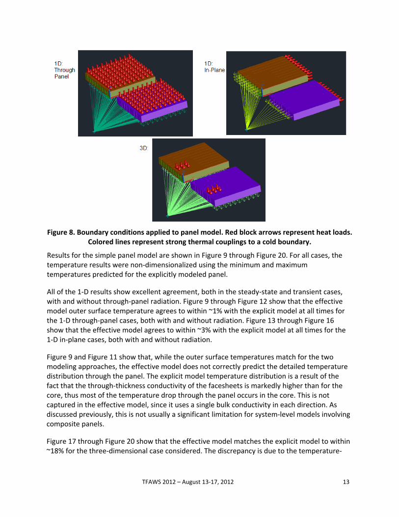
Figure 8. Boundary conditions applied to panel model. Red block arrows represent heat loads. Colored lines represent strong thermal couplings to a cold boundary. 

Results for the simple panel model are shown in Figure 9 through Figure 20. For all cases, the temperature results were non‐dimensionalized using the minimum and maximum temperatures predicted for the explicitly modeled panel. 

All of the 1‐D results show excellent agreement, both in the steady‐state and transient cases, with and without through‐panel radiation. Figure 9 through Figure 12 show that the effective model outer surface temperature agrees to within ~1% with the explicit model at all times for the 1‐D through‐panel cases, both with and without radiation. Figure 13 through Figure 16 show that the effective model agrees to within ~3% with the explicit model at all times for the 1‐D in‐plane cases, both with and without radiation. 

Figure 9 and Figure 11 show that, while the outer surface temperatures match for the two modeling approaches, the effective model does not correctly predict the detailed temperature distribution through the panel. The explicit model temperature distribution is a result of the fact that the through‐thickness conductivity of the facesheets is markedly higher than for the core, thus most of the temperature drop through the panel occurs in the core. This is not captured in the effective model, since it uses a single bulk conductivity in each direction. As discussed previously, this is not usually a significant limitation for system‐level models involving composite panels. 

Figure 17 through Figure 20 show that the effective model matches the explicit model to within ~18% for the three‐dimensional case considered. The discrepancy is due to the temperature‐

 

  TFAWS 2012 – August 13‐17, 2012  13  

 

  TFAWS 2012 – August 13‐17, 2012  14  

spreading effect of the relatively high‐conductivity facesheets, which is not captured in the effective model for reasons discussed above. Fortunately, thermal loads on system‐level aerospace models usually vary in a gradual way spatially; i.e., point loads as modeled here are not typical. Also, by not modeling the thermal spreading effect of higher‐conductivity facesheets, the effective model will predict more extreme outer surface temperatures and temperature gradients, which is usually conservative. Finally, this problem is most pronounced for low‐conductivity cores with higher‐conductivity facesheets. Figure 21 and Figure 22 show that if the Nomex core is replaced with higher‐conductivity aluminum honeycomb, the effective model matches the explicit model to within ~7% for the three‐dimensional case considered, both with and without radiation. 

  

Figure 9. Simple panel model steady‐state results for 1‐D through‐panel case without radiation. 

 

  TFAWS 2012 – August 13‐17, 2012  15  

 

Figure 10. Simple panel model transient results for 1‐D through‐panel case without radiation. 

 

  TFAWS 2012 – August 13‐17, 2012  16  

 

Figure 11. Simple panel model steady‐state results for 1‐D through‐panel case with radiation. 

 

  TFAWS 2012 – August 13‐17, 2012  17  

 

Figure 12. Simple panel model transient results for 1‐D through‐panel case with radiation. 

 

  TFAWS 2012 – August 13‐17, 2012  18  

 

Figure 13. Simple panel model steady‐state results for 1‐D in‐plane case without radiation. 

 

  TFAWS 2012 – August 13‐17, 2012  19  

 

Figure 14. Simple panel model transient results for 1‐D in‐plane case without radiation. 

 

  TFAWS 2012 – August 13‐17, 2012  20  

  

Figure 15. Simple panel model steady‐state results for 1‐D in‐plane case with radiation. 

 

  TFAWS 2012 – August 13‐17, 2012  21  

 

Figure 16. Simple panel model transient results for 1‐D in‐plane case with radiation. 

 

  TFAWS 2012 – August 13‐17, 2012  22  

 

Figure 17. Simple panel model steady‐state results for 3‐D case without radiation. 

 

  TFAWS 2012 – August 13‐17, 2012  23  

 

Figure 18. Simple panel model transient results for 3‐D case without radiation. 

 

  TFAWS 2012 – August 13‐17, 2012  24  

 

Figure 19. Simple panel model steady‐state results for 3‐D case with radiation. 

 

  TFAWS 2012 – August 13‐17, 2012  25  

 

Figure 20. Simple panel model transient results for 3‐D case with radiation. 

 

  TFAWS 2012 – August 13‐17, 2012  26  

 

Figure 21. Simple panel model transient results for 3‐D case without radiation and with an aluminum core. 

 

  TFAWS 2012 – August 13‐17, 2012  27  

 

Figure 22. Simple panel model transient results for 3‐D case with radiation and with an aluminum core. 

CONCLUSIONS 

We have developed a method to semi‐automatically import system‐level structural models containing arbitrary numbers of composite layups into Thermal Desktop. The method was used successfully to create a system‐level model of a commercial spacecraft containing hundreds of composite layups. 

The method accommodates complex geometries and will correctly orient the effective layup materials on the analysis mesh. Layups can contain any number of layers, and the layers can have orthotropic, temperature‐dependent properties and arbitrary ply orientations. The method also accounts for through‐thickness conduction, which is often important for composite panels. 

Comparison of a simple panel model created using the method to an explicitly modeled panel demonstrated that the method does an outstanding job of predicting transient and steady‐state temperatures for one‐dimensional load cases, but caution should be exercised if a given system will be subjected to markedly three‐dimensional loadings, such as point loads. For one‐dimensional loadings, the simplified model response matched the detailed model to within 3%, 

 

  TFAWS 2012 – August 13‐17, 2012  28  

 

  TFAWS 2012 – August 13‐17, 2012  29  

while the model response matched to within 7 to 18% for a point loading, depending on the relationship between panel facesheet and core conductivity. (High‐conductivity facesheets combined with low‐conductivity cores resulted in the worst performance.) 

We feel that this performance is adequate for a majority of system‐level models of aerospace structures and recommend its use when faced with systems containing otherwise‐daunting numbers of composite panels. 

ACKNOWLEDGEMENTS 

We would like to thank Cullimore and Ring Technologies for their lightning‐fast responses to our requests for new features and bug fixes in Thermal Desktop. 

CONTACT 

Matt Garrett is a thermal engineer in the Colorado office of the consulting firm ATA Engineering, Inc., headquartered in San Diego. He is currently responsible for system‐level thermal analysis of a crewed space vehicle. Previously, Mr. Garrett was employed by Goodrich Aerostructures in San Diego and by MDA Space Missions in Canada. He was the lead thermal engineer for the Shuttle Remote Manipulator System (SRMS) and the Orbiter Boom Sensor System Integrated Boom Assembly (OBSS IBA). He received his M.S. in Mechanical Engineering from Queen’s University in Canada. Mr. Garrett can be contacted at 303.945.2367 or matt.garrett@ata‐e.com. 

Victoria Harris is a mechanical engineer for ATA in San Diego.  Ms. Harris’s work is focused on structural analysis, and she has participated in a range of projects from space vehicles to amusement park rides.  She received her M.S. in Mechanical Engineering from the University of California, San Diego. Ms. Harris can be contacted at 858.480.2186 or victoria.harris@ata‐e.com. 

Alanna Koser recently received her B.S. in Mechanical Engineering from the University of Washington. While attending university, she participated in two 3‐month co‐op sessions with ATA, during which she gained experience in structural and thermal analysis via methods such as Finite Element and Finite Difference Analysis. In September she will begin working for Intel Corporation in DuPont, Washington. 

NOMENCLATURE, ACRONYMS, ABBREVIATIONS 

1‐D, 2‐D, 3‐D  One‐dimensional, two‐dimensional, three‐dimensional 

ATA    ATA Engineering, Inc. 

C    Specific heat 

 

  TFAWS 2012 – August 13‐17, 2012  30  

C&R    Cullimore and Ring Technologies 

CHEXA   Nastran hexahedral element definition 

CORD2R  Nastran coordinate system definition 

FD    Finite difference 

FE    Finite element 

FEM    Finite element model 

k    Thermal conductivity 

m    Mass 

MAT5/MATT5 Nastran orthotropic, temperature‐dependent thermal material definition 

MID    Nastran material identification number 

OOP    Out‐of‐plane 

PCOMP  Nastran composite property definition 

PID    Nastran property identification number 

PSOLID   Nastran solid property definition 

T    Nastran ply thickness 

t    Layer thickness 

T‐D    Thermal Desktop 

THETA    Nastran ply orientation angle 

TPS    Thermal protection system 

ρ    Density 

θ    Layer orientation angle 

Subscripts 

eff    Effective property 

m, mx, my  Referring to the layer coordinate system 

 

  TFAWS 2012 – August 13‐17, 2012  31  

p    Constant pressure 

xx, yy    Referring to the layup coordinate system 

…

REFERENCES 

1. Garrett, M. and Koser, A., “A Method for Importing Multiple Nastran Composite Layups into Thermal Desktop,” ATA Engineering, presented at The Aerospace Corp. 2012 Spacecraft Thermal Control Workshop, March 20–22, 2012. 

2. Herbert, G.W., “Diagram of a Composite Sandwich Panel,” Wikipedia, Sept 2006. 

3. “NX Nastran 8 Quick Reference Guide,” Siemens Product Lifecycle Management Software Inc., 2011. 

4. NX 8 Documentation, Siemens Product Lifecycle Management Software Inc., 2011. 

5. “Thermal Desktop, A CAD Based System for Thermal Analysis and Design, ver 5.5,” Cullimore and Ring Technologies, 2012. 

6. http://www.altairhyperworks.com 

7. “I‐DEAS User’s Guide,” Siemens Product Lifecycle Management Software Inc., 2010. 

8. http://www.mathworks.com 

9. http://www.ata‐e.com/software/imat 

10. Hibbeler, R.C., “Statics and Mechanics of Materials,” Prentice‐Hall, Inc., Englewood Cliffs, New Jersey, 1993.