HAL Id: hal-02351167https://hal.archives-ouvertes.fr/hal-02351167

Preprint submitted on 13 Nov 2019

HAL is a multi-disciplinary open accessarchive for the deposit and dissemination of sci-entific research documents, whether they are pub-lished or not. The documents may come fromteaching and research institutions in France orabroad, or from public or private research centers.

L’archive ouverte pluridisciplinaire HAL, estdestinée au dépôt et à la diffusion de documentsscientifiques de niveau recherche, publiés ou non,émanant des établissements d’enseignement et derecherche français ou étrangers, des laboratoirespublics ou privés.

A method to estimate horse speed at canter from IMUdata with Machine Learning

Amandine Schmutz, Laurence Chèze, Julien Jacques, Pauline Martin

To cite this version:Amandine Schmutz, Laurence Chèze, Julien Jacques, Pauline Martin. A method to estimate horsespeed at canter from IMU data with Machine Learning. 2019. �hal-02351167�

A method to estimate horse speed at canter from IMU data with Machine LearningAuthors: Amandine Schmutz, Laurence Cheze, Julien Jacques, Pauline Martin

1 IntroductionAccording to Article 234 of the FEI Jumping Rules, horses speed for internationalcompetitions has to be 350 m per minute minimum and 400 m per minute max-imum, with exceptions for different kinds of show conditions (FEI, FEI JumpingRules, 26th edition, 2019). Speed is therefore a key parameter for success in show-jumping competitions and an important training input.

3D optical motion capture is currently the gold standard for horse gait anal-ysis and can be therefore used for measuring stride parameters such as speed (Pfau,Witte, and Wilson, 2005). Nevertheless, the setting up of the measurement field istime consuming as well as data processing when your subject differs from the plug-in gait reference provided by the software (van der Kruk and Reijine, 2018). Thoseaspects make its use impossible on a daily basis or during championships for a riderwho wants descriptive results of his horse performance and locomotion parameterswithin a minute and potentially in real time without preliminary preparation.New gait analysis techniques emerged and enabled the development of tools to pro-vide objective parameters of horse’s motion (Martin, Cheze, Pourcelot, Desquilbet,Duray, and Chateau, 2017) or to detect lameness (Pfau, Boultbee, Davis, Walker,and Rhodin, 2016), using low-cost inertial measurement units (IMU), composedof two sensors: tri-axial accelerometer and tri-axial gyroscope. Those sensors canbe coupled with tri-axial magnetometer, and are therefore called mIMU. Thanks todata fusion techniques, the use of a magnetometer helps reducing the IMU bias andleads to better estimation of distance (Filippeschi, Schmitz, Miezal, Bleser, Ruf-faldi, and Stricker, 2017). IMUs can also be paired with Global Positioning System(GPS) unit, to improve the estimation of locomotion parameters such as speed (Tan,Wilson, and Lowe, 2008, Zihajehzadeh, Loh, Lee, Hoskinson, and Park, 2015).Nevertheless, GPS measurements can be badly influenced by the presence of obsta-cles (Wing, Eklund, and Kellogg, 2005) and it cannot be used indoors due to signalloss under roofing.

There exist three main families of methods developed to calculate motioncharacteristics from IMU signals. Firstly, model-based methods, like inverted pen-dulum models for speed estimation in human gait, which simplifies complex biome-chanical behaviors with simple mechanical model and incorporates subject-specificinformation like the limb length (Duong and Suh, 2017, Murphy, Carr, and O’Neill,2010). Secondly, signal-based methods which mainly rely on signal integration(Brzostowski, 2018) and use signal processing methods like Butterworth filter to

prevent drifting (Bosch, Serra Braganca, Marin-Perianu, Marin-Perianu, Van derZwaag, Voskamp, Back, Van Weeren, and Havinga, 2018). Those methods needto formulate some realistic assumptions to correct sensors drift and need a zero-velocity phase within each stride to be able to apply the integration process. Forexample the method proposed by Pfau et al. (2005) estimates horse displacementfrom one IMU placed on the trunk, assuming that the horse is in a steady statebecause of a treadmill that constrained the horse motion. In this case, the IMUsensor displacement should follow a closed loop and then the average velocity overa stride should be zero, as well as the average forward-backward and side-to-sideacceleration. Thus, in this context, stride-by-stride mean subtraction of accelera-tion and of the calculated velocity before integration enables determination of theintegration constants. This assumption is often invalid in numerous experimentalconditions, leading to the non-applicability of direct signal integration method. Thethird family of methods is more recent and based on statistical approaches, origi-nally developed to estimate human speed from IMUs data (Sabatini and Mannini,2016, Zihajehzadeh and Park, 2017). Those approaches provide accurate estima-tion of walking speed but regression models accuracy seems to be dependent of therange of motion. To prevent the drift, a first step is proposed where data are dividedaccording to their speed regime, thanks to a Support Vector Machine (SVM, Bishop(2006)), before the computation of speed by regression model (Zihajehzadeh, Aziz,Tae, and Park, 2018). Thus, the regression model is fit independently to each rangeof speed. This method refines the regression model accuracy for slow speed regime.Statistical methods concept is simple: one has to provide a dataset, called trainingdataset, with known variable of interest value (for example, IMU signals matchedto their associated speed) that will be used to build a model. The model will thenbe able to predict the value of the variable of interest for new data. The model hasto be trained with cases that can be encountered in its future application, withoutwhich it will perform poorly. We want to extend those methods to the horse motion.

The objective of this work is to develop a smart device that can provide therider with the movement parameters of his horse, in daily routine such as duringtraining sessions as well as during competition events, using only one IMU fixed inthe saddle. The idea is also to propose a tool that overcomes the limits imposed bythe use of GPS or 3D optical motion capture systems. This user-case differs fromexisting published work for sports (Camomilla, Bergamini, Fantozzi, and Vannozzi,2018) by not using sensors fusion, not being in a steady state that allows an easy useof direct integration of acceleration signals, nor using a sensor on the limb whichallows to reset errors at each cycle on short time periods.

In order to do so, several machine learning models and different data confor-mations will be tested. The obtained results will be compared to those of one signalbased method, already used for speed estimation in animal locomotion, the Overall

Dynamic Body Acceleration. The aimed accuracy is 0.6 m/s (36 m/min) in orderto meet the expectations of the show jumping professionals. As far as the authorsknow, this accuracy has not been reached for horses by the previously mentionedmethods using data from one IMU only (Pfau et al., 2005, Bosch et al., 2018).

2 Materials and methods

2.1 Data

The database used for model development is made of 3221 canter strides from 58ridden jumping horses of different breeds, height (129-176 cm), age (5-18 years old)and different levels of competition (amateur or professional). One IMU (LSM6DSL,STMicroelectronics) placed in the saddle close to the horse’s withers was used tomeasure tri-axial acceleration (range ±8 g) and tri-axial rotation rate (range ±2000dps) at a sampling frequency of 100 Hz. Data collected by the IMU were sent viaa Bluetooth R© antenna to a smartphone (iPhone X, Apple Inc.) and then stored onan online server. Two different protocols, which will be detailed here-after, wereused to collect data: the first one was speed measurement for a straight path andthe second one was speed measurement for a curved path. For both protocols, ref-erence speed was measured by video cameras or chronometer and matched to eachstride signal to train the machine learning model. For each protocol, “strides” weredefined from the maximum peak on the Z-axis (cf. Figure 1) of the raw accelera-tion data to the next 100 samples, in order to have the same number of points foreach individual regardless the speed, a necessary condition to use machine learningmethods. So, depending on the horse’s speed, this data segmentation may includemore than one cycle. We choosed not to re-sample a cycle in order to keep theinformation on the duration of the stride to estimate speed. Values from the threeaxes of the gyroscope and the accelerometer were extracted according to this cut-ting process with an automated detection algorithm written in MATLAB (R2014b).

2.1.1 Straight path

To get reference stride speed, IMU data were synchronized to a 4-cameras 2D track-ing system (UI-5240CP-M-GL, IDS) which had a measuring field of 26 meters.Horses were equipped with ten 2D-reflecting markers on anatomical landmarks(Figure 2) and their speed in the camera’s field was derived from the markers’2D trajectories using a custom software written on MATLAB R© (R2014b). Theaccuracy of this system is of 1.4% of the measured distance (Martin, 2015), which

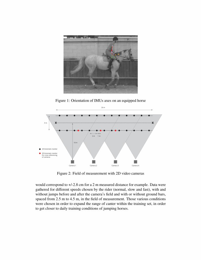
Figure 1: Orientation of IMUs axes on an equipped horse

26 m

2 m

4 m

Camera 1 Camera 2 Camera 3 Camera 4

2D kinematic marker2D kinematic markerfor cross referencingof cameras

1 m

10 m

Figure 2: Field of measurement with 2D video cameras

would correspond to +/-2.8 cm for a 2 m measured distance for example. Data weregathered for different speeds chosen by the rider (normal, slow and fast), with andwithout jumps before and after the camera’s field and with or without ground bars,spaced from 2.5 m to 4.5 m, in the field of measurement. Those various conditionswere chosen in order to expand the range of canter within the training set, in orderto get closer to daily training conditions of jumping horses.

Starting point chronometer TAG HEUER

Finish point chronometer TAG HEUER

Cones

Ground bar

15 m of diameter

3 m

7,5 m

Figure 3: Plan of speed measurement on curves for a horse at left-hand canter

2.1.2 Curved path

Because the 2D tracking system has a good accuracy only when the horse dis-placement is perpendicular to the cameras field, another measurement protocol wasdesigned for curve displacement. A curved path of known perimeter was definedwith cones and with a width small enough to make the horses pass the measuringequipment in a rather narrow path (Figure 3). The traveled distance was calculatedas distance = 2πr, with r the radius of the circle. Time spent in the curve by thehorse was measured with an automatic chronometer (CP 520, Tag Heuer) triggeredat the entrance and at the exit of the curved path (Figure 3). The average speedof the horse was then derived as speed = distance/time. Each stride of the horsewithin the curve was then matched with the average speed. For example, if theaverage speed in the curve was 6 m/s and the horse did 5 strides, then a speed of6 m/s was assumed for all these strides. In order to mimic real-life conditions of ajumping course the whole database is composed of 2906 strides collected in straightpath and 315 strides in curved path.

2.2 Speed measurement methods

2.2.1 Overall Dynamic Body Acceleration method

Overall Dynamic Body Acceleration (ODBA) method is a signal-based method pro-posed in Wilson, White, Quintana, Halsey, Liebsch, Martin, and Butler (2006) thatdoes not rely on signal integration. They developed a parameter named ODBA,calculated from acceleration in the 3 space directions, which is closely linked to thespeed of a walking animal.In our case, acceleration signals are low-pass filtered using a fourth-order Butter-worth filter with a cut-off frequency of 10 Hz. After that, an angle correction isapplied to align the Z-axis with the gravity vector. Then for each axis, as specifiedby Wilson et al. (2006), the signal mean value is subtracted from smoothed data.Those values are then converted to absolute positive units. Finally, resulting signalsare summed up and a mean ODBA value is calculated for each stride. A linearregression is then used to link the mean ODBA for one stride to the speed of thestride. The linear regression is performed with R software (v.3.4.0) (R Core Team,2017a) and the lm function of stats package (R Core Team, 2017b).

2.2.2 Statistical models

In a mathematical point of view monitored signals can be considered into two dif-ferent ways. The first approach is as a multi-dimensional vector of size 606 (101values per measured signal). The second approach is a vector of six functional vari-ables, one per measured signal. The main advantage of considering collected dataas a vector of functional variables is that we keep the temporal dynamic. We referto Ramsay and Silverman (2005) for univariate and bivariate examples.

The statistical methods we have tested can be divided into two categories.The first one, high dimensional models which deal with data sets where the numberof columns can be large. Among those methods we tested Ridge regression, Lassoregression, Principal Component Regression (PCR), Partial Least Square regression(PLS), Elastic net regression, neural network, random forest and Support VectorMachine (SVM). For a complete review about these models refer to (Bishop, 2006,Hastie, Tibshirani, and Friedman, 2001). Secondly, the functional approaches witha parametric regression model for functional data (Ramsay and Silverman, 2005)and a non parametric regression model (Ferraty and Vieu, 2006).

As in Zihajehzadeh et al. (2018), we wonder if the division of the databaseinto smaller homogeneous subgroups, before the computation of speed by the re-gression model may improve the model accuracy. Thus, each previously describedmodel will be tested on raw data and on the database divided into two subgroups.

These subgroups has been built thanks to a clustering method for multivariate func-tional data (Schmutz, Jacques, Bouveyron, Cheze, and Martin, 2018).

Figure 4: Diagram of statistical methods process from training to the speed predic-tion

To sum up, the signals collected with the accelerometer and the gyroscopefor each stride are matched with the measured reference speed. This is used asinput data to train the model in order to obtain the best speed estimation for newdata in the future. All this process is illustrated on Figure 4. Models are devel-oped with R software (v.3.4.0) and packages glmnet (Friedman, Hastie, and Tib-shirani, 2010), pls (Mevik, Wehrens, and Liland, 2016), neuralnet (Fritsch andGuenther, 2016), randomForest (Liaw and Wiener, 2002), e1071 (Meyer, Dimitri-adou, Hornik, Weingessel, and Leisch, 2017), fda.usc (Febrero-Bande and Oviedode la Fuente, 2012), funHDDC (Schmutz and Bouveyron, 2019) and function funo-pare.knn.lcv (Ferraty and Vieu, 2006).

2.2.3 Methods comparison

To compare the accuracy of methods, the database is cut into two parts: a trainingdataset which is composed of a random sampling of 80% of the database, and theremaining 20% forms the test dataset. The models are built on the training dataset

and their accuracy is then evaluated on the test dataset. Evaluating methods on anindependent test dataset prevents over-fitting.

Comparison between models is done with the calculation of the percentageerror in the estimated speed above 0.6 m/s. This threshold is the minimum satis-factory for this parameter to make sense for the professionals. Percentage error iscomputed as:

% error = 100×∑i

|Measured speed at stridei−Predicted speed at stridei|> 0.6Total number of strides

,

with i corresponding to each stride of the test dataset.Then, the best machine learning model and ODBA model are also compared

with Bland and Altman plots and its 95% limits of agreement (Bland and Altman,1999), which allows the evaluation of differences between two methods used onthe same individuals (here strides). In our case, we examine the average differencebetween each method and reference values obtained with 2D tracking system forstraight path and chronometer for curve path. Bland and Altman analysis and graphsare built with the bland.altman.plot function from the BlandAltmanLeh R package(Lehnert, 2015).

3 ResultsTo avoid results fluctuation due to random sampling of the test dataset, the randomsampling process of the database is repeated 50 times and the average, minimumand maximum of percentage error are estimated for each repetition on raw data.When data are divided into two subgroups, the weighted mean, minimum and max-imum is computed.

Table 1 shows the mean results for each model. The division of raw data intosubgroups improves results of percentage of error for all high dimensional regres-sion models, ODBA method and, to a lesser extend, neural network and parametricfunctional regression. Nevertheless, the best results are obtained with SVM methodapplied on raw data. SVM clearly outperforms its competitors.

The Bland and Altman plot of one SVM repetition is shown on Figure 5(top), where one point corresponds to one stride. The speed predicted by the modeland the measured speed of the stride are compared. The mean bias is 0, whichmeans that in average the SVM model output is close to the measured speed. If themodel predictions were perfect, all the points would be aligned on the zero line.The points that are the farthest from the zero line are the worst predictions. We cansee that for some strides of low speed (below 5 m/s), the SVM model has a tendencyto overestimate their speed. Whereas for some strides of high speed (above 5 m/s),

the SVM model has a tendency to underestimate themWhereas ODBA estimations(Figure 5, bottom) are more variable than SVM ones. The mean bias is also 0 butthe 95% confidence interval is twice the size of SVM one (cf. Table 1), that isto say high above our objective value. The ODBA method is more variable thanthe SVM one, with 95% of strides bias lower than 2.5 m/s and a clear tendency tounderestimate strides of high speed.

−7.5

−5.0

−2.5

0.0

2.5

2 4 6 8 10

Measured and predicted speed (m/s)

Bia

s (m

/s)

SVM method

−7.5

−5.0

−2.5

0.0

2.5

2 4 6 8 10

Measured and predicted speed (m/s)

Bia

s (m

/s)

ODBA method

Figure 5: Bland and Altman plot for one repetition of SVM model with its 95%confidence interval (top) and ODBA method (bottom)

Raw data SubgroupsMethod Mean Min Max Mean Min MaxRidge 27.7 24.2 30.7 24.0 21.2 27.6Lasso 29.1 25.9 31.8 25.0 22.0 28.1PCR 28.5 25.5 31.1 26.4 21.2 34.8PLS 28.8 25.0 32.2 26.4 21.0 33.8

Elastic net α = 0.3 27.9 24.6 30.9 24.1 21.0 27.7Parametric functional regression 26.9 23.6 31.7 26.4 23.1 29.4

Non parametric functional regression 16.7 13.0 20.1 17.2 14.9 20.3SVM 9.9 6.7 11.9 10.7 7.8 12.8

Neural network 29.9 25.7 33.7 28.7 24.8 34.8Random Forest 17.5 14.3 20.7 18.3 14.7 20.7

ODBA 51.4 47.8 55.1 47.8 28.6 68.6

Table 1: Mean, minimum and maximum values of percentage of error above 0.6m/s for speed estimation

4 Discussion and ConclusionThe objective of our study was to develop a model which can be integrated into asmart device in order to accurately provide horse speed per stride to the rider. Thissmart device is made of only one IMU situated on the horse wither. The number ofsensors is kept to a minimum in order to facilitate the daily use of this tool and thenon-use of GPS is due to our willingness to make this tool work both indoors andoutdoors.

In this work, we propose to use machine learning models to predict horsespeed from IMU data. On the collected dataset, Support Vector Machine gave thebest results which the lowest percentage of error (above 0.6 m/s). SVM methodoutperformed other machine learning models and ODBA method. ODBA is a signalbased method that does not need external inputs to estimate speed per stride fromnew IMU data. Indeed, direct signal integration methods, which are commonly usedin human case or in horses running on a treadmill case, need strong assumptions tocalculate an integration constant for speed estimation that cannot be made whenthe horse moves in real conditions and when the IMU is not located on the limb(Filippeschi et al., 2017, Camomilla et al., 2018). Moreover, biomechanical modelshave not been developed for an asymmetrical gait such as horse canter.

The superiority of machine learning models in this work can be partly ex-plain by the fact that, usually, models for speed estimation first detect a stride, then

cut the collected signal according to this stride and apply the calculation model(Bichler, Ogris, Kremser, Schwab, Knott, and Baca, 2012, Mannini and Sabatini,2014, Zhao, Brahms, Gerhard, and Barden, 2016). These methods standardized thestride duration for all individuals and few of them take into account the stride du-ration to calculate speed parameter leading to a loss of information. In the presentwork, we choose a different way of pre-processing the collected signals. Indeed,the stride is detected on the Z-axis but 101 points are kept from the maximal peakon Z-axis. This change allows to keep the stride duration information: for highspeed the ”stride” will have a signal that contain more canter cycles than low speed”strides”. This data pre-processing helps increasing the accuracy of the statisticalmodel.

The novelty of the present work is to propose a model for speed estimationthat relies on one IMU only. The integration of machine learning model in a de-vice for equestrian sport is innovative in comparison with other existing systemsfor equestrian sports based on GPS or in comparison with human tracking motionsystems that are mainly based on the use of a magnetometer or several IMUs (Fil-ippeschi et al., 2017). The machine learning approach allows the development ofa smart device that does not rely on a GPS for the estimation of a physical phe-nomenon, here the horse speed at each stride, with an accuracy of 0.6 m/s. This ac-curacy meets the expectations of professionals of show jumping discipline, whichwas their main concern about using or not connected devices. Indeed, as showjumping can be practiced both indoors and outdoors, our tool overcomes the GPSsystems limitations. Moreover, the accuracy of our model can easily be refined byperforming more campaigns of measurement with the reference systems. Indeed,a panel of 58 horses is not sufficient to model the behavior of all horses due toindividual’s diversity. It is also necessary to do more measurements on curves ofvarious diameters, since it greatly influences the horse’s behavior, the correspond-ing collected signals and therefore the horse speed (Greve and Dyson, 2016).

We cannot benchmark our model to other works on horses because no oneelse provides a speed per stride estimation. Indeed, Pfau et al. (2005) and Boschet al. (2018) calculate traveled distance with its preciseness but Bosch et al. (2018)aim to provide a speed estimation in future work. Whereas in human researches,a wide literature exists on computing human walking speed from data collectedby one IMU placed on the foot, as for example Mannini and Sabatini (2014) whocompare two methods of walking speed estimation, whose accuracy is between0.5 km/h (0.14 m/s) and 0.7 km/h (0.19 m/s) depending on the walking speed andthe method used. Zihajehzadeh and Park (2016) develop a model for walking speedestimation based on a regression model which use data from one wrist-worn inertialsensor. In their paper, the Bland and Altman limits of agreements are lower than 0.2m/s. Sabatini and Mannini (2016) estimate an instantaneous velocity decomposed

in the three space directions from two IMUs placed one on the pelvis and the otheron the shank of the subject, its accuracy is in the same range than the one of previousstudies. For instance, considering a walking man of 3 km/h (0.8 m/s), the error ofthe previous models is around 27% whereas for a running show jumping horseof 350 m/min (5.8 m/s) our model error is about 10%. Thus, our model is moreaccurate than the existing ones for human walking.

Another advantage of our model is that it can be transferred to another disci-pline than show jumping as long as consistent data are provided to train the model.Indeed, show jumping canter is specific to the discipline where the bounce is im-portant whereas in endurance horses, flat canter is preferred. Therefore, in order toadapt our tool to other disciplines, the model has to be expanded with more datagathered in new situations. The SVM model is transposable to the other equestriansports and to bipedal locomotion, as long as consistent data are provided to trainthe model.

To conclude, the predictive method shown herein above is accurate becausethe reference data, used as a training dataset, were collected with great precisionand are consistent with the model application (show jumping).

ReferencesBichler, S., G. Ogris, V. Kremser, F. Schwab, S. Knott, and A. Baca (2012): “To-

wards high-precision imu/gps-based stride-parameter determination in an out-door runners’ scenario,” 9th Conference of the International Sports EngineeringAssociation (ISEA), 34, 592–597.

Bishop, C. M. (2006): Pattern Recognition and Machine Learning (InformationScience and Statistics), Berlin, Heidelberg: Springer-Verlag.

Bland, J. M. and D. G. Altman (1999): “Measuring agreement in method compari-son studies,” Statistical Methods in Medical Research, 8, 135–160.

Bosch, S., F. Serra Braganca, M. Marin-Perianu, R. Marin-Perianu, B. J. Van derZwaag, J. Voskamp, W. Back, R. Van Weeren, and P. Havinga (2018):“Equimoves: A wireless networked inertial measurement system for objectiveexamination of horse gait,” Sensors, 18.

Brzostowski, K. (2018): “Novel approach to human walking speed enhancementbased on drift estimation,” Biomedical Signal Processing and Control, 42, 18 –29.

Camomilla, V., E. Bergamini, S. Fantozzi, and G. Vannozzi (2018): “Trends sup-porting the in-field use of wearable inertial sensors for sport performance evalu-

ation: A systematic review,” Sensors, 18.Duong, H. T. and Y. S. Suh (2017): “Walking distance estimation of a walker user

using a wrist-mounted imu,” in 2017 56th Annual Conference of the Society ofInstrument and Control Engineers of Japan (SICE), 1061–1064.

Febrero-Bande, M. and M. Oviedo de la Fuente (2012): “Statistical computing infunctional data analysis: The R package fda.usc,” Journal of Statistical Software,51, 1–28.

Ferraty, F. and P. Vieu (2006): Nonparametric functional data analysis, SpringerSeries in Statistics, New York: Springer.

Filippeschi, A., N. Schmitz, M. Miezal, G. Bleser, E. Ruffaldi, and D. Stricker(2017): “Survey of motion tracking methods based on inertial sensors: A focuson upper limb human motion,” Sensors, 17.

Friedman, J., T. Hastie, and R. Tibshirani (2010): “Regularization paths for gener-alized linear models via coordinate descent,” Journal of Statistical Software, 33,1–22.

Fritsch, S. and F. Guenther (2016): neuralnet: Training of Neural Networks.Greve, L. and S. Dyson (2016): “Body lean angle in sound dressage horses in-hand,

on the lunge and ridden,” Veterinary journal, 217, 52–57.Hastie, T., R. Tibshirani, and J. Friedman (2001): The Elements of Statistical Learn-

ing, Springer Series in Statistics, New York, NY, USA: Springer New York Inc.Lehnert, B. (2015): BlandAltmanLeh: Plots (Slightly Extended) Bland-Altman

Plots.Liaw, A. and M. Wiener (2002): “Classification and regression by randomforest,”

R News, 2, 18–22.Mannini, A. and A. Sabatini (2014): “Walking speed estimation using foot-mounted

inertial sensors: comparing machine learning and strap-down integration meth-ods,” Medical engineering and physics, 36, 1312–1321.

Martin, P. (2015): Saddle In Motion : back biomechanics of the ridden horse : anal-ysis of the interactions between the saddle and the back, and application to thedevelopment of news prototypes of saddles, Theses, Universite Claude Bernard -Lyon I.

Martin, P., L. Cheze, P. Pourcelot, L. Desquilbet, L. Duray, and H. Chateau (2017):“Effects of the rider on the kinematics of the equine spine under the saddle duringthe trot using inertial measurement units: Methodological study and preliminaryresults,” Veterinary Journal, 221, 6–10.

Mevik, B.-H., R. Wehrens, and K. H. Liland (2016): pls: Partial Least Squares andPrincipal Component Regression.

Meyer, D., E. Dimitriadou, K. Hornik, A. Weingessel, and F. Leisch (2017): e1071:Misc Functions of the Department of Statistics, Probability Theory Group (For-merly: E1071), TU Wien.

Murphy, J., H. Carr, and M. O’Neill (2010): “Animating horse gaits and transi-tions,” in E. UK, ed., Symposium on Theory and Practice of Computer Graphics.

Pfau, T., H. Boultbee, H. Davis, A. Walker, and M. Rhodin (2016): “Agreementbetween two inertial sensor gait analysis systems for lameness examinations inhorses,” Equine Veterinary Education, 28, 203–208.

Pfau, T., T. Witte, and A. Wilson (2005): “A method for deriving displacement dataduring cyclical movement using an inertial sensor,” The Journal of experimentalbiology, 208, 2503–2514.

R Core Team (2017a): R: A Language and Environment for Statistical Com-puting, R Foundation for Statistical Computing, Vienna, Austria, URLhttps://www.R-project.org/.

R Core Team (2017b): R: A Language and Environment for Statistical Computing,R Foundation for Statistical Computing, Vienna, Austria.

Ramsay, J. O. and B. W. Silverman (2005): Functional data analysis, SpringerSeries in Statistics, New York: Springer, second edition.

Sabatini, A. M. and A. Mannini (2016): “Ambulatory assessment of instantaneousvelocity during walking using inertial sensor measurements,” Sensors, 16.

Schmutz, A. and J. J. . C. Bouveyron (2019): funHDDC: Univariate and Multivari-ate Model-Based Clustering in Group-Specific Functional Subspaces, r packageversion 2.3.0.

Schmutz, A., J. Jacques, C. Bouveyron, L. Cheze, and P. Martin (2018): “Clus-tering multivariate functional data in group-specific functional subspaces,” URLhttps://hal.inria.fr/hal-01652467, working paper or preprint.

Tan, H., A. Wilson, and J. Lowe (2008): “Measurement of stride parameters usinga wearable gps and inertial measurement unit,” Journal of biomechanics, 41,1398–1406.

van der Kruk, E. and M. Reijine (2018): “Accuracy of human motion capture sys-tems for sport applications; state-of-the-art review,” European Journal of SportScience, 18, 806–819.

Wilson, R., C. White, F. Quintana, L. Halsey, N. Liebsch, G. Martin, and P. Butler(2006): “Moving towards acceleration for estimates of activity-specific metabolicrate in free-living animals: the case of the cormorant,” Journal of Animal Ecol-ogy, 75, 1081–1090.

Wing, M. G., A. Eklund, and L. D. Kellogg (2005): “Consumer-Grade Global Posi-tioning System (GPS) Accuracy and Reliability,” Journal of Forestry, 103, 169–173.

Zhao, Y., M. Brahms, D. Gerhard, and J. Barden (2016): “Stance phase detectionfor walking and running using an imu periodicity-based approach,” in P. Chung,A. Soltoggio, C. W. Dawson, Q. Meng, and M. Pain, eds., Proceedings of the10th International Symposium on Computer Science in Sports (ISCSS), Cham:

Springer International Publishing, 225–232.Zihajehzadeh, S., O. Aziz, C. Tae, and E. J. Park (2018): “Combined regression and

classification models for accurate estimation of walking speed using a wrist-wornimu,” in 2018 40th Annual International Conference of the IEEE Engineering inMedicine and Biology Society (EMBC), 3272–3275.

Zihajehzadeh, S., D. Loh, T. J. Lee, R. Hoskinson, and E. J. Park (2015): “Acascaded kalman filter-based gps/mems-imu integration for sports applications,”Measurement, 73, 200 – 210.

Zihajehzadeh, S. and E. J. Park (2016): “Regression model-based walking speedestimation using wrist-worn inertial sensor,” PLOS ONE, 11, 1–16.

Zihajehzadeh, S. and E. J. Park (2017): “A gaussian process regression model forwalking speed estimation using a head-worn imu,” in 2017 39th Annual Inter-national Conference of the IEEE Engineering in Medicine and Biology Society(EMBC), 2345–2348.