A Microbenchmark Case Study and Lessons Learned

Joseph (Yossi) Gil Keren Lenz∗

Yuval ShimronDepartment of Computer Science

The Technion—Israel Institute of TechnologyTechnion City, Haifa 3200, Israel

AbstractThe extra abstraction layer posed by the virtual machine, the JITcompilation cycles and the asynchronous garbage collection are themain reasons that make the benchmarking of Java code a delicatetask. The primary weapon in battling these is replication: “billionsand billions of runs”, is phrase sometimes used by practitioners.This paper describes a case study, which consumed hundreds ofhours of CPU time, and tries to characterize the inconsistencies inthe results we encountered.

Keywordsbenchmark, measurements, steady-state

1. IntroductionScience is all about the generation of new and verifiable truths. Inexperimental sciences, this amounts to reproducible experimenta-tion. In experimental computer science, reproducibility may seemeasy, since we are accustomed to deterministic and predictable com-puting systems: We expect that hitting a key labeled ‘a’ shall al-ways, in a bug-free environment, produce the letter ‘a’ on the screen.

It came therefore as a surprise to the authors of this paper thatin our attempt to benchmark a certain small JAVA [1] function, atask known as micro-benchmarking, we encountered inconsistentresults, even after neutralizing effects of well known perturbing fac-tors such as garbage collection, just in time compilation, dynamicloading, and operating system background processes.

This paper tells the story of our micro-benchmarking endeavors,and tries to characterize the inconsistencies we encountered. Lit-tle effort is spent on trying to explain these; we believe this taskrequires a dedicate study which would employ different researchtools (simulation and hardware probes come to mind). Our hopeis that this report would contribute to better understanding of thephenomena we describe and promote the development of methodsto eliminate these.

∗contact author: lkeren@cs.technion.ac.il

VMIL ’11 October 24, 2011, Portland, Oregon.

1.1 Background: Benchmarking and Micro-benchmarking of Java

Benchmarking of computer systems is a notoriously delicate task [9].The increasingly growing abstraction gap between programs andtheir execution environments, most notably virtual machines, forcesbenchmarking, which could, in the early days, be carried out bycounting program instructions, to use methods used in experimen-tal, exact and social sciences.

Other issues brought about by the widening abstraction layer in-clude the fact that the same benchmark on different platforms mayyield different, and even contradictory results [4]. In addition, dif-ferent compilers may apply different optimizations to source code,and therefore comparing two alternatives compiled with one com-piler can lead to different results than the comparison of the samealternatives compiled using a different compiler.

Micro-benchmarking, measuring the performance of a piece of code(as opposed to assessing the performance of an application) is evenmore challenging. There are several subtle issues that can cause abenchmarker to draw wrong conclusions from an experiment. Onesuch aspect is the use of dead code: micro-benchmarks often donothing but calling the benchmarked code. Compilers may recog-nize such pattern and eliminate parts of the benchmark code, lead-ing to code that runs faster than expected. In order to avoid that, it isnot enough just to call the benchmarked code, but some extra codehas to be introduced in the benchmark. However, doing so leads toa benchmark which measures the performance of the original andthe extra code, introducing noise into the measurement.

Micro-benchmarking of JAVA functions raises its own set of in-triguing issues.1 There are two major hurdles for JAVA microbench-marks: First, the Just In Time (JIT) compiler, may change the codeas it executes. Secondly, the Garbage Collector (GC) may asyn-chronously consume CPU cycles during the benchmark. Multi-threading may also be a concern, given the fact that an ordinaryJava Virtual Machine (JVM) invocation, even of a non-threadedprogram, spawns a dozen of threads in addition to the main thread.

JIT compiles methods to different optimization levels, and is drivenby timer-based sampling. Thus, in different runs different sam-ples may be taken, leading to different methods being optimized atdifferent levels, and to variations in running time of a benchmarkacross different JVM invocations, even on a single host [2].

1See Clikc’s JavaOne’02 presentation, “How NOT To Writea Microbenchmark?”, www.azulsystems.com/events/-javaone 2002/microbenchmarks.pdf

The first iterations of the benchmarked code include a large amountof dynamic compilation. Later iterations are usually faster bothsince they include less compilation and because the executed codeis compiled and optimized [7]. The common wisdom of dealingwith the presence of the JIT compiler is by conducting, prior to thebeginning of the benchmark, warm-up executions of the benchedcode. The warm-up stage should be sufficiently long to allow theJIT compiler to fully compile and optimize the benchmarked code.

In dealing with the GC, one can allocate sufficiently large heapspace to the JVM to reduce the likelihood of GC. Also, the inter-mittent nature of the GC effect on the results can be averaged byrepeating the benchmark sufficiently many times.

The main tool of the trade is then replication: “billions and billionsof runs”, is the phrase sometimes used by practitioners. But, as wediscovered, there are certain contributions to inconsistency whichcould not be mitigated by simple replication.

1.2 FindingsHaving eliminated as much as we could the effects of JIT com-pilation, GC cycles and operating system and other environmen-tal noise, we conducted benchmarking experiments consisting of avery large number of runs. Our case study revealed at least fourdifferent factors that contributed to inconsistency in the results:

1. Instability of the Virtual Machine. We show that different,seemingly identical invocations of the virtual machine maylead to different results, and that this difference (which maybe in the order of 3%) is statistically significant. The impactof this instability may be more significant when two compet-ing implementations are compared.This variation increases with the abstraction level, in the sensethat when the JIT compiler is disabled, the discrepancy be-tween different VM invocations increases.Observe that naive replication, within the same VM cannotimprove the accuracy of the results. The remedy is in repli-cation of the VMs.

2. Multiple Steady States. We observed that in some invoca-tions, the VM converges to a certain steady state, and then,within the same invocation, leaps into a different steady state.The consequence of this phenomenon is that an averagedmeasurement within a single VM invocation may be mislead-ing in not reflecting or characterizing these leaps.

3. Multiple Simultaneous Steady States. Further, we observedthat in some invocations, the VM converges to two or moresimultaneous steady states, in the sense that a given mea-surement has high probability of assuming one of number ofdistinct results, and small probability of assuming any inter-mediate value. A simple average of these results may be evenmore misleading report of the benchmarking process.

4. Prologue Effects. Finally, we demonstrate that the running-time of the benchmarked code may be significantly affectedby execution of unrelated prologue code, and that this effectpersists even if the benchmarked code is executed a greatnumber of times. This means that one cannot reliably bench-mark two distinct pieces of code in a single program execu-tion.The more disturbing conclusion is that the timing results ob-tained in a clean benchmarking environment may be mean-ingless when the benchmarked code is used in an application.

Even if the application executes this code numerous times,the (unknown) application prologue effects may persist, ren-dering the benchmarked results meaningless.

1.3 Related WorkNon-determinism of benchmarking results is a well studied area.It is well known that modern processors are chaotic in the math-ematical sense, and therefore analyzing the performance behaviorof a complex program on a modern processor architecture is a dif-ficult task [3]. Eechout et al. [6] showed that benchmarking resulthighly depends on the virtual machine; results obtained for one VMmay not be obtained by another VM. Blackburn et al [4] showedthat a JAVA performance evaluation methodology should considermultiple heap sizes and multiple hardware platforms, in addition toconsidering multiple JVMs.

Several attempts were made to suggest methodologies for bench-marking. One particularly interesting and increasingly widely usedmethodology replay compilation [10], which is used to control thenon-determinism that stems from compilation and optimization.The main idea is the creation of a “compilation plan”, based ona series of training runs and then the use of this plan to determinis-tically apply optimizations.

Georges, Buytaert and Eeckhout [7] describe prevalent performanceanalysis methodologies and point their statistical pitfalls. The pa-per presents a statistically robust method for measuring both startuptime and steady-state performance.

Blackburn et al. [5] recommend methodologies for performanceevaluation in the presence of non-determinism introduced by dy-namic optimization and garbage collection in managed languages.Their work stresses the importance of choosing a meaningful base-line, to which the benchmark results are compared, and controllingfree variables such as hosts, runtime environments, heap size andwarm-up time. To deal with non-determinism the authors suggeststhree strategies: (i) using replay compilation, (ii) measuring per-formance in steady state, with JIT compiler turned off, and (iii)generating multiple results and apply statistical analysis to these.

Mytkowicz, Diwan, Hauswirth and Sweeney [12] discuss factorswhich cause measurement bias, suggest statistical methods drawnfrom natural and social sciences to detect and avoid it. To avoidbias, the paper suggests a method which is based on applying alarge number of randomized experimental setup, and using statisti-cal methods to analyze the results. The method for detecting bias,causal analysis, is a technique used for establishing confidence thatthe conclusions drawn from the collected data are valid.

Lea, Bacon and Grove [11] claim that there is a need to establish asystematic methodology for measuring performance, and to teachstudents and researchers this methodology.

Georges et al. [8] present a technique for measuring processor-level information gathered through performance counters and link-ing that information to specific methods in a JAVA program. Theyargue that “different methods are likely to result in dissimilar be-havior and different invocations of the same method are likely toresult in similar behavior”.

Outline. The remainder of this paper is organized as follows. InSection 2 we describe the setting of our experimental evaluation,the hardware and software used, and the benching environment.

Section 3 shows that different, seemingly identical, invocations ofthe JVM may converge to distinct steady states. This finding is fur-ther examined in Section 4, which also shows that the discrepancyis greater when the JIT compiler is not present. Section 5 showsthat even a single JVM invocation may have multiple steady states,and that, further, these multiple steady states may be simultaneous.The impact of prologue execution is the subject of Section 6. Sec-tion 7 concludes and suggests directions for further research.

2. Settings of the Benchmark2.1 Hardware and Software EnvironmentTo minimize effects of disk swapping and background processeson benchmarking, we selected a computer with a large RAM andmultiple cores. Measurements were conducted on a Lenovo Think-Centre desktop computer, whose configuration is as follows: an In-tel Core 2 Quad CPUQ9400 processor (i.e., a total of four cores),running at 2.66 GHz and equipped with 8GB of RAM. Hosts usedin specific experiments are described below.

During benchmarking all cores were placed in “performance” mode,thereby disabling clock rate and voltage changes.

On this computer, we installed Ubuntu version 10.04.2 (LTS) andthe readily available open JAVA development kit (OpenJDK, IcedTea61.9.8) including version 1.6.0 20 of the JAVA Virtual Machine (specif-ically 6b20-1.9.8-0ubuntu1˜10.04.1). Other software environmentsused in specific experiments are described below.

To minimize interruptions and bias due to operating system back-ground (and foreground) processes, all measurements took placewhile the machine was running in what’s called “single-user” mode(telinit 1), under root privileges in textual teletype interaction(no GUI), and with networking disabled.

2.2 Benchmark AlgorithmOur atomic unit of benchmarked code was defined as an instanceof a class implementing interface Callable (defined in packagejava.util.concurrent). This interface defines a single no-arguments method, which returns an Object value.

Given an implementation of Callable our benchmark algorithmworks in three stages: (i) estimation, (ii) warm-up, and (iii) mea-surement. The purpose of the estimation phase is to obtain a veryrough estimate of execution time of the parameter. In the warm-upstage, this estimation is used for warming up the given Callable,i.e., iterating it until the JIT compiler has realized its full potential,for a specified warm-up period (five seconds in our experiments).In the measurement phase, the running time of the parameter ismeasured repeatedly. Each such measurement executes the param-eterm times, wherem is so selected that the measurement durationis roughly that of a parameter τ .

All phases are based on making a number of sequences of itera-tions of the Callable object parameter. Each iteration sequenceis monitored for garbage collection cycles, JIT compilation cy-cles, and class loading/unloading events by probing the MX-beansfound in class ManagementFactory (which is defined in pack-age java.lang.management). The timing result of a sequenceis discarded if any of these events happen. Further, the detection ofJIT compilation cycles late in the warm-up period, increases its du-ration. And, the repeated detection of garbage collection cyclestriggers shortening of a measurement sequence so as to decreasethe likelihood of further interruptions of this sort.

2.3 Benchmarked CodeAt the focus of our attention we placed the implementation of classHashMap, arguably one of the most popular classes of the JAVAruntime environment. We used version 1.73 of the code, (datedMarch 13, 2007) due to Doug Lea, Josh Bloch, Arthur van Hoffand Neal Gafter. To preclude the option of pre-optimization of codepresent in JAVA libraries, we benchmarked a copy of the code in ourbenchmarking library.

Within this class, we concentrated in the throughput of functionV get(Object key) which retrieves the value associated witha key stored in the hash table. Listing 1 depicts this function’s code.

Listing 1 Java code for benchmarked function (function get inclass HashMap)

1 public V get(Object key) {2 if (key == null) return getForNullKey();3 int hash = hash(key.hashCode());4 for (5 Entry<K,V> e=table[hash & table.length-1];6 e != null;7 e = e.next8 ) {9 Object k;

10 if (11 e.hash == hash12 &&13 ( (k = e.key) == key14 ||15 key.equals(k)16 )17 )18 return e.value;19 }20 return null;21 }

This function includes iterations, conditionals and logical opera-tions, array access and pointer dereferencing. Examining functionhash which is called by get in line 3 (Listing 2), we see that thebenchmarked code includes also bit operations.

Listing 2 JAVA code for function hash (invoked from get in classHashMap)

static int hash(int h) {h ˆ= h >>> 20 ˆ h >>> 12;return h ˆ h >>> 7 ˆ h >>> 4;

}

Our measurements never pass a null argument, so there is no needto examine the code of function getForNullKey. Also, we onlyexercise get in searching for keys which are not present in the hashtable. The call key.equals(k) is thus executed only in the casethat the cached hash value (field hash in the entry) happens to beequal to the hash value of the searched key. This rare event doesnot happen in our experiments, so, the call key.equals(k) isnever executed.

All in all, the benchmarked code is presented in its entirety in list-ings 1 and 2. Notably, the benchmarked code does not include any

virtual function calls—foregoing virtual optimization techniques.Viable optimization techniques include e.g., branch prediction, pre-fetching, inlining, and elimination of main memory access opera-tions. Also, the code does not allocate memory, nor does it changethe value of any reference. As it turns out, there was not a singlegarbage collection cycle in a sequence of one billion consecutivecalls to function get.

The precise manner in which get was exercised was as follows:

1. Fix n = 1, 152.

2. Make n pairs of type 〈key, value〉 , where both the Stringkey and the Double value are selected using a random num-ber generator started with a fixed seed.

3. Create an empty HashMap<String, Double> data struc-ture and populate it with these pairs.

4. Create an array of n fresh keys of type String, where keysare selected using the same random number generator.

5. The benchmarked procedure, getCaller(), then iteratesover the keys array, calling get for each of its elements.

6. The throughput of function get is defined as the running-time of getCaller() divided by n.

3. No Single Steady StateWe conducted v = 7 independent invocations of our benchmarkingprogram, i.e., each invocation uses a freshly created VM. These in-vocations were consecutive, with a script invoking the VM v times.

In each invocation the VM carried out r = 20, 000 iterations, i.e., rexecutions of the measurement procedure described above (after asingle estimation stage followed by a single warm-up stage). Weshall call such an iteration a measurement session. A measurementsession returns a measurement result (result for short).

A measured result of t (for function getCaller()) gives a through-put of t/n for function get(). Also, a measurement session oflength τ calls getCaller() about τ/t times. The throughput inour experiment was about 15.3ns per each get() call.

Overall, in our case, τ/t ≈ 6, 000. If the time of each of the it-erations of getCaller() were independent, then, by the centrallimit theorem the r results collected in an invocation should be closeto a normal distribution.

Overall, in the experiment described in this section, the number ofexecutions of function get, was about

v × r × 100ms15.3ns× 1, 152

≈ 0.8× 109

Table 1 summarizes the essential statistics of the distribution ofmeasurement results in our experiment. (The “mad” column repre-sents the median of absolute deviations from the median—a statis-tics which is indicative of the quality of the median statistics androbust to outliers.)

The values in each column, i.e., the same statistics of different invo-cations, appear quite similar. The median is close to the mean; thesestatistics indicate a throughput of about 15.2–15.3ns/operation. Thestandard deviation is about 0.1ns, which is about 0.7% of the mean.

No. Mean σ Median Mad Min Max1 15.27 0.0802 15.27 0.0509 14.95 15.692 15.17 0.0768 15.17 0.0454 14.74 15.693 15.24 0.0726 15.24 0.0451 14.93 15.674 15.38 0.0727 15.38 0.0430 15.06 15.815 15.29 0.0867 15.30 0.0495 14.95 15.686 15.10 0.0722 15.11 0.0420 14.83 15.517 15.24 0.0929 15.25 0.0559 14.87 15.60

Table 1: Essential statistics (in ns/operation) of the distributionof measurement results in seven consecutive invocations of a20,000 iterations measurement, τ = 100ms .

The extreme values appear to be well behaved in that they deviatefrom the mean by about 5%.

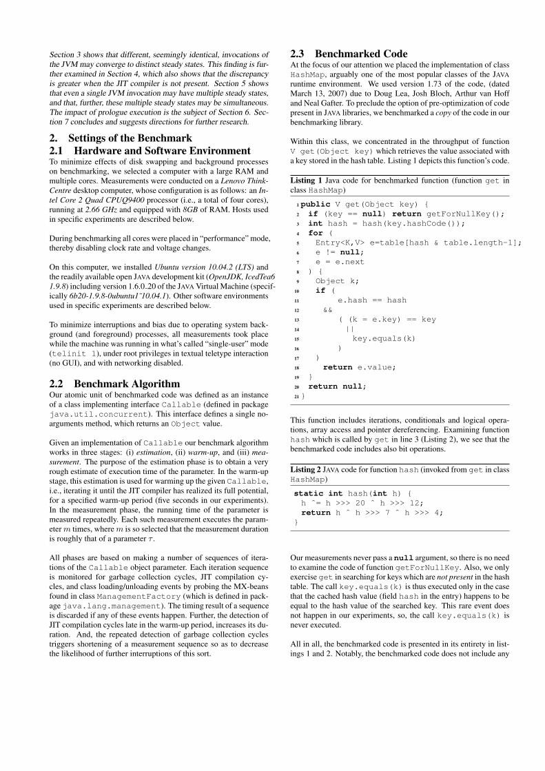
The mean throughput in the different invocations spans a 0.28ns ≈2% range which may seem reasonable. A graphical plot of the dis-tribution of the same results, as done in Figure 1, reveals a some-what different picture. A quick look at the figure, suggests thatthe results in two different invocations are drawn from close, yetdistinct, distributions.

0

2

4

6

8

10

14.6 14.8 15 15.2 15.4 15.6 15.8 16

Dis

tribu

tion

Den

sity

Throughput [ns/op]

Figure 1: Distribution of benchmark results in seven invoca-tions of a 20,000 iterations experiment, τ = 100ms

Each curve in the figure represents the distribution function of the rvalues obtained in a single invocation. Here, and henceforth, allcurves were smoothed out by using a kernel density estimation,where a Gaussian was used as the windowing function, and wherea bandwidth free parameter was h (lower values means less estima-tion). The value of h selected in all figures is

h = mini

4

3r

1/5

σi,

where i ranges over all distribution plotted in the same figure, σi be-ing the standard deviation of the ith distribution. (In normal, Gaus-sian distribution, the optimal value of h is (4/3r)1/5σ.)

Also, here and henceforth, the smoothed distribution was scaleddown by multiplying the density by 1/r, so as to make the totalarea under the curve 1.

A quick “back of an envelope” analysis confirms that the differ-ence between the means of the different invocations is statisticallysignificant.

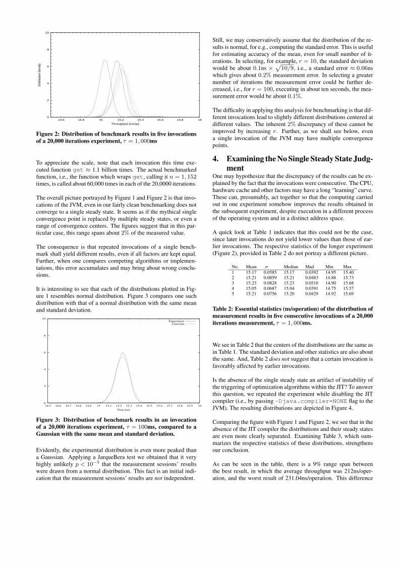
To increase certainty in our findings, we repeated the experimentwith τ = 1, 000ms = 1sec, except that for practical reasons, weset v = 5. The resulting distributions are depicted in Figure 2.

0

2

4

6

8

10

14.6 14.8 15 15.2 15.4 15.6 15.8 16

Dis

tribu

tion

Den

sity

Throughput [ns/op]

Figure 2: Distribution of benchmark results in five invocationsof a 20,000 iterations experiment, τ = 1, 000ms

To appreciate the scale, note that each invocation this time exe-cuted function get ≈ 1.1 billion times. The actual benchmarkedfunction, i.e., the function which wraps get, calling it n = 1, 152times, is called about 60,000 times in each of the 20,0000 iterations.

The overall picture portrayed by Figure 1 and Figure 2 is that invo-cations of the JVM, even in our fairly clean benchmarking does notconverge to a single steady state. It seems as if the mythical singleconvergence point is replaced by multiple steady states, or even arange of convergence centers. The figures suggest that in this par-ticular case, this range spans about 2% of the measured value.

The consequence is that repeated invocations of a single bench-mark shall yield different results, even if all factors are kept equal.Further, when one compares competing algorithms or implemen-tations, this error accumulates and may bring about wrong conclu-sions.

It is interesting to see that each of the distributions plotted in Fig-ure 1 resembles normal distribution. Figure 3 compares one suchdistribution with that of a normal distribution with the same meanand standard deviation.

0

2

4

6

8

10

14.5 14.6 14.7 14.8 14.9 15 15.1 15.2 15.3 15.4 15.5 15.6 15.7 15.8 15.9 16

Time [ns]

ExperimentGaussian

Figure 3: Distribution of benchmark results in an invocationof a 20,000 iterations experiment, τ = 100ms, compared to aGaussian with the same mean and standard deviation.

Evidently, the experimental distribution is even more peaked thana Gaussian. Applying a JarqueBera test we obtained that it veryhighly unlikely p < 10−5 that the measurement sessions’ resultswere drawn from a normal distribution. This fact is an initial indi-cation that the measurement sessions’ results are not independent.

Still, we may conservatively assume that the distribution of the re-sults is normal, for e.g., computing the standard error. This is usefulfor estimating accuracy of the mean, even for small number of it-erations. In selecting, for example, r = 10, the standard deviationwould be about 0.1ns ×

√10/9, i.e., a standard error ≈ 0.06ns

which gives about 0.2% measurement error. In selecting a greaternumber of iterations the measurement error could be further de-creased, i.e., for r = 100, executing in about ten seconds, the mea-surement error would be about 0.1%.

The difficulty in applying this analysis for benchmarking is that dif-ferent invocations lead to slightly different distributions centered atdifferent values. The inherent 2% discrepancy of these cannot beimproved by increasing r. Further, as we shall see below, evena single invocation of the JVM may have multiple convergencepoints.

4. Examining the No Single Steady State Judg-ment

One may hypothesize that the discrepancy of the results can be ex-plained by the fact that the invocations were consecutive. The CPU,hardware cache and other factors may have a long “learning” curve.These can, presumably, act together so that the computing carriedout in one experiment somehow improves the results obtained inthe subsequent experiment, despite execution in a different processof the operating system and in a distinct address space.

A quick look at Table 1 indicates that this could not be the case,since later invocations do not yield lower values than those of ear-lier invocations. The respective statistics of the longer experiment(Figure 2), provided in Table 2 do not portray a different picture.

No. Mean σ Median Mad Min Max1 15.17 0.0585 15.17 0.0392 14.95 15.402 15.21 0.0859 15.21 0.0483 14.88 15.733 15.23 0.0828 15.23 0.0510 14.90 15.684 15.05 0.0687 15.04 0.0391 14.75 15.575 15.21 0.0756 15.20 0.0429 14.92 15.69

Table 2: Essential statistics (ns/operation) of the distribution ofmeasurement results in five consecutive invocations of a 20,000iterations measurement, τ = 1, 000ms.

We see in Table 2 that the centers of the distributions are the same asin Table 1. The standard deviation and other statistics are also aboutthe same. And, Table 2 does not suggest that a certain invocation isfavorably affected by earlier invocations.

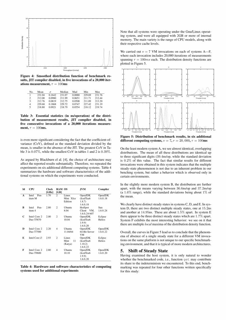
Is the absence of the single steady state an artifact of instability ofthe triggering of optimization algorithms within the JIT? To answerthis question, we repeated the experiment while disabling the JITcompiler (i.e., by passing -Djava.compiler=NONE flag to theJVM). The resulting distributions are depicted in Figure 4.

Comparing the figure with Figure 1 and Figure 2, we see that in theabsence of the JIT compiler the distributions and their steady statesare even more clearly separated. Examining Table 3, which sum-marizes the respective statistics of these distributions, strengthensour conclusion.

As can be seen in the table, there is a 9% range span betweenthe best result, in which the average throughput was 212ns/oper-ation, and the worst result of 231.04ns/operation. This difference

0

2

4

6

8

10

215 220 225 230

Dis

tribu

tion

Den

sity

Throughput [ns/op]

Figure 4: Smoothed distribution function of benchmark re-sults, JIT compiler disabled, in five invocations of a 20,000 iter-ations measurement, τ = 100ms

No. Mean σ Median Mad Min Max1 231.04 0.1642 231.07 0.0888 229.69 231.762 212.00 0.0980 211.99 0.0651 211.71 212.443 212.76 0.0819 212.75 0.0508 211.89 213.204 229.68 0.1868 229.72 0.0747 227.42 231.195 218.80 0.0921 218.79 0.0554 218.12 219.74

Table 3: Essential statistics (in ns/operation) of the distri-bution of measurement results, JIT compiler disabled, infive consecutive invocations of a 20,000 iterations measure-ment, τ = 100ms.

is even more significant considering the fact that the coefficient-of-variance (CoV), defined as the standard deviation divided by themean, is smaller in the absence of the JIT. The greatest CoV in Ta-ble 3 is 0.07%, while the smallest CoV in tables 1 and 2 is 0.39%.

As argued by Blackburn el al. [4], the choice of architecture mayaffect the reported results substantially. Therefore, we repeated theexperiments on six additional different computing systems. Table 4summarizes the hardware and software characteristics of the addi-tional systems on which the experiments were conducted.

Id CPU Clock[GHz]

RAM[GB]

OS JVM Compiler

A Intel Pen-tium M

1.70 2 LinuxMint XfceEdition

OpenJDK(IcedTea61.8.7)1.6.0 18

OpenJDK1.6.0 18

B Intel Pen-tium 4

2.80 2 Ubuntu8.04

HotSpotClient VM,1.6.0 24-b07

Sun1.6.0 24

C Intel Core 2Duo T5870

2.00 2 Ubuntu10.04

OpenJDK(IcedTea61.9.9)1.6.0 20

EclipseHelios

D Intel Core 2Duo T7500

2.20 4 Ubuntu11.04/64

OpenJDK64-Bit ServerVM

OpenJDK1.6.0 22

E Intel Core i3 2.93 2 LinuxMint 11(Katya)

OpenJDK(IcedTea61.10.2)1.6.0 22

EclipseHelios

F Intel Core 2Duo T9600

2.80 4 Ubuntu10.10

OpenJDK(IcedTea61.9.9)1.6.0 20

OpenJDK1.6.0 20

Table 4: Hardware and software characteristics of computingsystems used for additional experiments

Note that all systems were operating under the Gnu/Linux operat-ing system, and were all equipped with 2GB or more of internalmemory. The main variety is the range of CPU models, along withtheir respective cache levels.

We carried out v = 7 VM invocations on each of systems A—F,where each invocation includes 20,000 iterations of measurementsspanning τ = 100ms each. The distribution density functions areplotted in Figure 5.

0

2

4

6

8

10

39 39.1 39.2 39.3 39.4 39.5 39.6

Throughput [ns/op]

A

0

2

4

6

8

10

35.5 36 36.5 37 37.5 38

Throughput [ns/op]

B

0

2

4

6

8

10

31.5 32 32.5 33 33.5

Throughput [ns/op]

C

0

2

4

6

8

10

14.6 14.8 15 15.2 15.4 15.6 15.8 16

Throughput [ns/op]

D

0

2

4

6

8

10

14.4 14.6 14.8 15 15.2 15.4

Throughput [ns/op]

E

0

2

4

6

8

10

12 12.5 13 13.5 14 14.5 15 15.5 16 16.5

Throughput [ns/op]

F

Figure 5: Distribution of benchmark results, in six additionaldifferent computing systems, v = 7, r = 20, 000, τ = 100ms

On the least modern system A, we see almost identical, overlappingdistributions. The mean of all these distributions are identical upto three significant digits (39.4ns/op, while the standard deviationis 0.2% of this value. The fact that similar results for differentinvocations were obtained in this system indicates that the multiplesteady-state phenomenon is not due to an inherent problem in ourbenching system, but rather a behavior which is observed only incertain environments.

In the slightly more modern system B, the distribution are furtherapart, with the means varying between 36.6ns/op and 37.2ns/op(a 1.6% range), while the standard deviations being about 1% ofthe mean.

We clearly have distinct steady states in systems C, D, and E. In sys-tem D, there are two distinct multiple steady states, one at 15.2nsand another at 14.95ns. These are about 1.5% apart. In system Ethere appear to be three distinct steady states which are 1.7% apart.System F exhibits the most interesting behavior: we see on it thatthere are multiple local maxima of the distribution density function.

Overall, the curves in Figure 5 lead us to conclude that the phenom-ena of absence of a single steady state for a different VM invoca-tions on the same platform is not unique to our specific benchmark-ing environment, and that it is typical of more modern architectures.

5. Shift of Steady StateHaving examined the host system, it is only natural to wonderwhether the benchmarked code, i.e., function get may contributeits share to the indeterminism we encountered. To this end, bench-marking was repeated for four other functions written specificallyfor this study:

1. arrayBubbleSort(), which randomly shuffles the val-ues in a fixed array of ints of size `1, and then resorts theseusing a simple bubble sort algorithm.

2. listBubbleSort(), which randomly shuffles the valuesin a fixed linked list of Integers of size `2 (without chang-ing the list itself), and then resorts these (again, without mod-ifying the list) using the same bubble sort algorithm.

3. xorRandoms(), which computes the X-OR of `3 consec-utive pseudo random integers drawn from JAVA’s standardlibrary random number generator.

4. recursiveErgodic(), which applies many recursive callsinvolving the creation and destruction of lists of integers,all implemented using the type ArrayList<Integer> tocreate an array of pseudo-ergodic sequence of length `4.

The implementation of these made the results of the computationexternally available so as to prevent an optimizing compiler fromoptimizing the loops out. Note that each of the four functions has itsown particular execution profile: Function arrayBubbleSortis characterized best by array access operations, while pointer deref-erencing is the principal characterization of listBubbleSort.Function xorRandoms() involves a lot of integer operations andis therefore mostly CPU bound, while memory allocation is themain feature of recursiveErgodic().

The values `1, `2, `3 and `4 were so selected to make the running-time of each of these four functions about the same as the func-tion that wraps get(). Thus, for τ = 100ms we have again about6,000 calls of the benchmarked function, and, we expect again ofthe sessions’ results to be normally distributed. Further, to make iteasier for humans to compare the results, we selected integers n1, n2, n3

and n4 and divided the resulting running-time values by these num-bers so as to make the “throughput” values close to those of thethroughput of get().

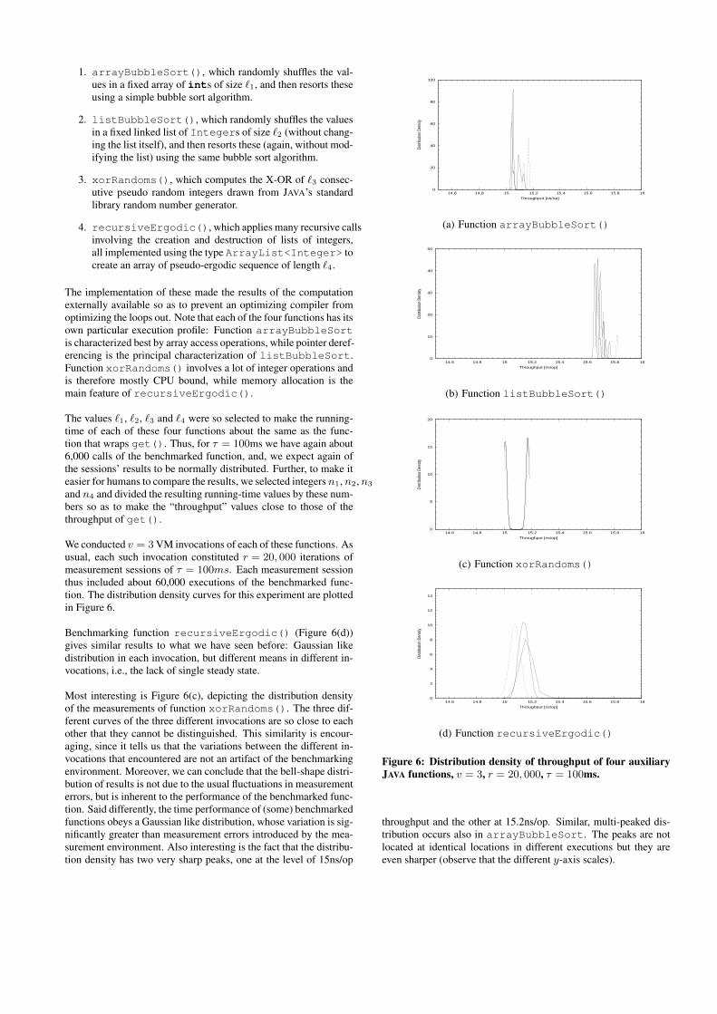
We conducted v = 3 VM invocations of each of these functions. Asusual, each such invocation constituted r = 20, 000 iterations ofmeasurement sessions of τ = 100ms. Each measurement sessionthus included about 60,000 executions of the benchmarked func-tion. The distribution density curves for this experiment are plottedin Figure 6.

Benchmarking function recursiveErgodic() (Figure 6(d))gives similar results to what we have seen before: Gaussian likedistribution in each invocation, but different means in different in-vocations, i.e., the lack of single steady state.

Most interesting is Figure 6(c), depicting the distribution densityof the measurements of function xorRandoms(). The three dif-ferent curves of the three different invocations are so close to eachother that they cannot be distinguished. This similarity is encour-aging, since it tells us that the variations between the different in-vocations that encountered are not an artifact of the benchmarkingenvironment. Moreover, we can conclude that the bell-shape distri-bution of results is not due to the usual fluctuations in measurementerrors, but is inherent to the performance of the benchmarked func-tion. Said differently, the time performance of (some) benchmarkedfunctions obeys a Gaussian like distribution, whose variation is sig-nificantly greater than measurement errors introduced by the mea-surement environment. Also interesting is the fact that the distribu-tion density has two very sharp peaks, one at the level of 15ns/op

0

20

40

60

80

100

14.6 14.8 15 15.2 15.4 15.6 15.8 16

Dist

ribut

ion

Dens

ity

Throughput [ns/op]

(a) Function arrayBubbleSort()

0

10

20

30

40

50

14.6 14.8 15 15.2 15.4 15.6 15.8 16

Dist

ribut

ion

Dens

ity

Throughput [ns/op]

(b) Function listBubbleSort()

0

5

10

15

20

14.6 14.8 15 15.2 15.4 15.6 15.8 16

Dist

ribut

ion

Dens

ity

Throughput [ns/op]

(c) Function xorRandoms()

0

2

4

6

8

10

12

14

14.6 14.8 15 15.2 15.4 15.6 15.8 16

Dist

ribut

ion

Dens

ity

Throughput [ns/op]

(d) Function recursiveErgodic()

Figure 6: Distribution density of throughput of four auxiliaryJAVA functions, v = 3, r = 20, 000, τ = 100ms.

throughput and the other at 15.2ns/op. Similar, multi-peaked dis-tribution occurs also in arrayBubbleSort. The peaks are notlocated at identical locations in different executions but they areeven sharper (observe that the different y-axis scales).

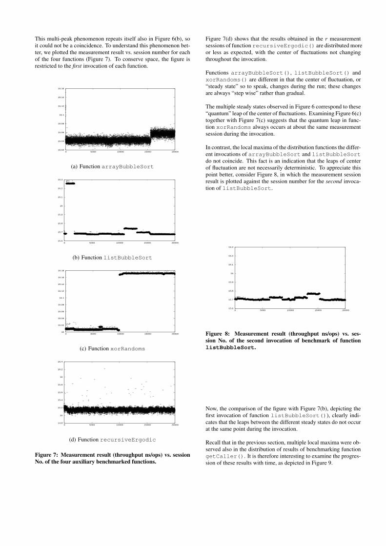
This multi-peak phenomenon repeats itself also in Figure 6(b), soit could not be a coincidence. To understand this phenomenon bet-ter, we plotted the measurement result vs. session number for eachof the four functions (Figure 7). To conserve space, the figure isrestricted to the first invocation of each function.

15.02

15.04

15.06

15.08

15.1

15.12

15.14

15.16

0 5000 10000 15000 20000

(a) Function arrayBubbleSort

15.6

15.7

15.8

15.9

16

16.1

16.2

16.3

0 5000 10000 15000 20000

(b) Function listBubbleSort

15

15.02

15.04

15.06

15.08

15.1

15.12

15.14

15.16

15.18

0 5000 10000 15000 20000

(c) Function xorRandoms

14.8

15

15.2

15.4

15.6

15.8

16

16.2

16.4

0 5000 10000 15000 20000

(d) Function recursiveErgodic

Figure 7: Measurement result (throughput ns/ops) vs. sessionNo. of the four auxiliary benchmarked functions.

Figure 7(d) shows that the results obtained in the r measurementsessions of function recursiveErgodic() are distributed moreor less as expected, with the center of fluctuations not changingthroughout the invocation.

Functions arrayBubbleSort(), listBubbleSort() andxorRandoms() are different in that the center of fluctuation, or“steady state” so to speak, changes during the run; these changesare always “step wise” rather than gradual.

The multiple steady states observed in Figure 6 correspond to these“quantum” leap of the center of fluctuations. Examining Figure 6(c)together with Figure 7(c) suggests that the quantum leap in func-tion xorRandoms always occurs at about the same measurementsession during the invocation.

In contrast, the local maxima of the distribution functions the differ-ent invocations of arrayBubbleSort and listBubbleSortdo not coincide. This fact is an indication that the leaps of centerof fluctuation are not necessarily deterministic. To appreciate thispoint better, consider Figure 8, in which the measurement sessionresult is plotted against the session number for the second invoca-tion of listBubbleSort.

15.6

15.7

15.8

15.9

16

16.1

16.2

16.3

0 5000 10000 15000 20000

Figure 8: Measurement result (throughput ns/ops) vs. ses-sion No. of the second invocation of benchmark of functionlistBubbleSort.

Now, the comparison of the figure with Figure 7(b), depicting thefirst invocation of function listBubbleSort()), clearly indi-cates that the leaps between the different steady states do not occurat the same point during the invocation.

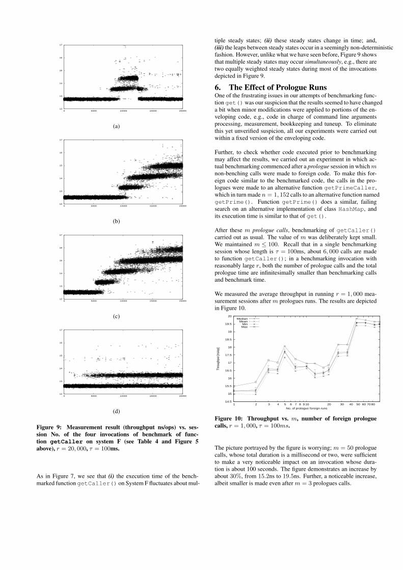
Recall that in the previous section, multiple local maxima were ob-served also in the distribution of results of benchmarking functiongetCaller(). It is therefore interesting to examine the progres-sion of these results with time, as depicted in Figure 9.

12

13

14

15

16

17

0 5000 10000 15000 20000

(a)

12

13

14

15

16

17

0 5000 10000 15000 20000

(b)

12

13

14

15

16

17

0 5000 10000 15000 20000

(c)

12

13

14

15

16

17

0 5000 10000 15000 20000

(d)

Figure 9: Measurement result (throughput ns/ops) vs. ses-sion No. of the four invocations of benchmark of func-tion getCaller on system F (see Table 4 and Figure 5above), r = 20, 000, τ = 100ms.

As in Figure 7, we see that (i) the execution time of the bench-marked function getCaller() on System F fluctuates about mul-

tiple steady states; (ii) these steady states change in time; and,(iii) the leaps between steady states occur in a seemingly non-deterministicfashion. However, unlike what we have seen before, Figure 9 showsthat multiple steady states may occur simultaneously, e.g., there aretwo equally weighted steady states during most of the invocationsdepicted in Figure 9.

6. The Effect of Prologue RunsOne of the frustrating issues in our attempts of benchmarking func-tion get()was our suspicion that the results seemed to have changeda bit when minor modifications were applied to portions of the en-veloping code, e.g., code in charge of command line argumentsprocessing, measurement, bookkeeping and tuneup. To eliminatethis yet unverified suspicion, all our experiments were carried outwithin a fixed version of the enveloping code.

Further, to check whether code executed prior to benchmarkingmay affect the results, we carried out an experiment in which ac-tual benchmarking commenced after a prologue session in whichmnon-benching calls were made to foreign code. To make this for-eign code similar to the benchmarked code, the calls in the pro-logues were made to an alternative function getPrimeCaller,which in turn made n = 1, 152 calls to an alternative function namedgetPrime(). Function getPrime() does a similar, failingsearch on an alternative implementation of class HashMap, andits execution time is similar to that of get().

After these m prologue calls, benchmarking of getCaller()carried out as usual. The value of m was deliberately kept small.We maintained m ≤ 100. Recall that in a single benchmarkingsession whose length is τ = 100ms, about 6, 000 calls are madeto function getCaller(); in a benchmarking invocation withreasonably large r, both the number of prologue calls and the totalprologue time are infinitesimally smaller than benchmarking callsand benchmark time.

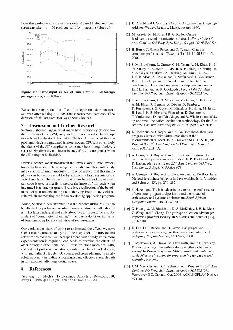
We measured the average throughput in running r = 1, 000 mea-surement sessions after m prologues runs. The results are depictedin Figure 10.

14.5

15

15.5

16

16.5

17

17.5

18

18.5

19

19.5

20

1 2 3 4 5 6 7 8 9 10 20 30 40 50 60 70 80

Thro

ughp

ut [n

s/op

]

No. of prologue foreign runs

MedianMean

MinMax

Figure 10: Throughput vs. m, number of foreign prologuecalls, r = 1, 000, τ = 100ms.

The picture portrayed by the figure is worrying; m = 50 prologuecalls, whose total duration is a millisecond or two, were sufficientto make a very noticeable impact on an invocation whose dura-tion is about 100 seconds. The figure demonstrates an increase byabout 30%, from 15.2ns to 19.5ns. Further, a noticeable increase,albeit smaller is made even after m = 3 prologues calls.

Does this prologue effect ever wear out? Figure 11 plots our mea-surements after m = 50 prologue calls for increasing values of r.

19.1

19.2

19.3

19.4

19.5

19.6

19.7

19.8

19.9

20

1000 10000 100000 1e+06

Thro

ughp

ut [n

s/op

]

Replications

MedianMean

MinMax

Figure 11: Throughput vs. No. of runs after m = 50 foreignprologue runs, τ = 100ms.

We see in the figure that the effect of prologue runs does not wearout even after making r = 128, 000 measurement sessions. (Theduration of this last execution was about 4 hours.)

7. Discussion and Further ResearchSection 3 showed, again, what many have previously observed—that a restart of the JVM, may yield different results. In attemptto study and understand this better (Section 4), we found that theproblem, which is aggravated in more modern CPUs, is not entirelythe blame of the JIT compiler as some may have thought before2;surprisingly, diversity and inconsistency of results are greater whenthe JIT compiler is disabled.

Delving deeper, we demonstrated that even a single JVM invoca-tion may have multiple convergence points, and this multiplicitymay even occur simultaneously. It may be argued that this multi-plicity can be compensated for by sufficiently large restarts of thevirtual machine. The concern is that micro-benchmarking of a cer-tain code is used primarily to predict the impact of this code whenintegrated in a larger program. Brute force replication of the bench-mark, without understanding the underlying issues, may yield re-sults which are meaningless for an enveloping application program.

Worse, Section 6 demonstrated that the benchmarking results canbe affected by prologue execution however infinitesimally short itis. This later finding, if not understood better (it could be a subtleartifact of “compilation planning”) may cast a doubt on the valueof benchmarking for the evaluation of real programs.

Our works stops short of trying to understand the effects we saw:such a task requires an analysis of the deep stack of hardware andsoftware abstractions. But, perhaps before such a study starts, moreexperimentation is required: one needs to examine the effects ofother prologue executions, no-JIT runs on other machines, with,and without prologue executions, study other benchmarked code,with and without JIT, etc. Of course, judicious planning is an ab-solute necessity in finding a meaningful and effective research pathin this exponentially huge design space.

8. References2see e.g., J. Bloch’s “Performance Anxiety”, Devoxx 2010,http://www.parleys.com/#st=5&id=2103

[1] K. Arnold and J. Gosling. The Java Programming Language.Addison-Wesley, Reading, Massachusetts, 1996.

[2] M. Arnold, M. Hind, and B. G. Ryder. Onlinefeedback-directed optimization of java. In Proc. of the 17th

Ann. Conf. on OO Prog. Sys., Lang., & Appl. (OOPSLA’02).

[3] H. Berry, D. Gracia Perez, and O. Temam. Chaos incomputer performance. Chaos, 16(1):013110–013110–15,2006.

[4] S. M. Blackburn, R. Garner, C. Hoffman, A. M. Khan, K. S.McKinley, R. Bentzur, A. Diwan, D. Feinberg, D. Frampton,S. Z. Guyer, M. Hirzel, A. Hosking, M. Jump, H. Lee,J. E. B. Moss, A. Phansalkar, D. Stefanovic, T. VanDrunen,D. von Dincklage, and B. Wiedermann. The DaCapobenchmarks: Java benchmarking development and analysis.In P. L. Tarr and W. R. Cook, eds., Proc. of the 21st Ann.Conf. on OO Prog. Sys., Lang., & Appl. (OOPSLA’06).

[5] S. M. Blackburn, K. S. McKinley, R. Garner, C. Hoffmann,A. M. Khan, R. Bentzur, A. Diwan, D. Feinberg,D. Frampton, S. Z. Guyer, M. Hirzel, A. Hosking, M. Jump,H. Lee, J. E. B. Moss, A. Phansalkar, D. Stefanovik,T. VanDrunen, D. von Dincklage, and B. Wiedermann. Wakeup and smell the coffee: evaluation methodology for the 21stcentury. Communications of the ACM, 51(8):83–89, 2008.

[6] L. Eeckhout, A. Georges, and K. De Bosschere. How javaprograms interact with virtual machines at themicroarchitectural level. In R. Crocker and G. L. S. Jr., eds.,Proc. of the 18th Ann. Conf. on OO Prog. Sys., Lang., &Appl. (OOPSLA’03).

[7] A. Georges, D. Buytaert, and L. Eeckhout. Statisticallyrigorous Java performance evaluation. In R. P. Gabriel andD. Bacon, eds., Proc. of the 22nd Ann. Conf. on OO Prog.Sys., Lang., & Appl. (OOPSLA’07).

[8] A. Georges, D. Buytaert, L. Eeckhout, and K. De Bosschere.Method-level phase behavior in Java workloads. In Vlissidesand Schmidt [13], pp. 270–287.

[9] S. Hazelhurst. Truth in advertising : reporting performanceof computer programs, algorithms and the impact ofarchitecture and systems environment. South AfricanComputer Journal, 46:24–37, 2010.

[10] X. Huang, S. M. Blackburn, K. S. McKinley, J. E. B. Moss,Z. Wang, and P. Cheng. The garbage collection advantage:improving program locality. In Vlissides and Schmidt [13],pp. 69–80.

[11] D. Lea, D. F. Bacon, and D. Grove. Languages andperformance engineering: method, instrumentation, andpedagogy. Sigplan Notices, 43:87–92, 2008.

[12] T. Mytkowicz, A. Diwan, M. Hauswirth, and P. F. Sweeney.Producing wrong data without doing anything obviouslywrong! In Proceeding of the 14th international conferenceon Architectural support for programming languages andoperating systems.

[13] J. M. Vlissides and D. C. Schmidt, eds. Proc. of the 19th Ann.Conf. on OO Prog. Sys., Lang., & Appl. (OOPSLA’04),Vancouver, BC, Canada, Oct. 2004. ACM SIGPLAN Notices39 (10).