A Model-Adaptive Universal Data Compression

Architecture with Applications to Image

Compression

by

Joshua Ka-Wing Lee

B.A.Sc. in Engineering Science, University of Toronto (2015)

Submitted to the Department of Electrical Engineering and ComputerScience in partial fulfillment of the requirements for the degree of

Master of Science in Computer Science and Engineering

at the

MASSACHUSETTS INSTITUTE OF TECHNOLOGY

June 2017

c○ Massachusetts Institute of Technology 2017. All rights reserved.

Author . . . . . . . . . . . . . . . . . . . . . . . . . . . . . . . . . . . . . . . . . . . . . . . . . . . . . . . . . . . . . . . .Department of Electrical Engineering and Computer Science

May 19, 2017

Certified by. . . . . . . . . . . . . . . . . . . . . . . . . . . . . . . . . . . . . . . . . . . . . . . . . . . . . . . . . . . .Gregory W. Wornell

Professor of Electrical Engineering and Computer ScienceThesis Supervisor

Accepted by . . . . . . . . . . . . . . . . . . . . . . . . . . . . . . . . . . . . . . . . . . . . . . . . . . . . . . . . . . .Leslie A. Kolodziejski

Professor of Electrical Engineering and Computer ScienceChair, Committee on Graduate Theses

2

A Model-Adaptive Universal Data Compression Architecture

with Applications to Image Compression

byJoshua Ka-Wing Lee

Submitted to the Department of Electrical Engineering and Computer Scienceon May 19, 2017, in partial fulfillment of the

requirements for the degree ofMaster of Science in Computer Science and Engineering

Abstract

In this thesis, I designed and implemented a model-adaptive data compression systemfor the compression of image data. The system is a realization and extension of theModel-Quantizer-Code-Separation Architecture for universal data compression whichuses Low-Density-Parity-Check Codes for encoding and probabilistic graphical modelsand message-passing algorithms for decoding. We implement a lossless bi-level imagedata compressor as well as a lossy greyscale image compressor and explain how thesecompressors can rapidly adapt to changes in source models. We then show using theseimplementations that Restricted Boltzmann Machines are an effective source modelfor compressing image data compared to other compression methods by comparingcompression performance using these source models on various image datasets.

Thesis Supervisor: Gregory W. WornellTitle: Professor of Electrical Engineering and Computer Science

3

4

Acknowledgments

I would like to extend my sincerest thanks to the many people without whose supportthis work would not have been completed.

First and foremost, I would like to thank my advisor Professor Gregory Wornell forhis guidance and teaching throughout my journey here at MIT. His advice has led meto the discovery of new ideas and fields that I would never have encountered otherwise.I owe much of my knowledge and passion for machine learning and information theoryto him, from lessons learned in the classroom to those gleaned from our meetings,and without his inspiration this project would never have existed in the first place.I am grateful beyond words for all he has done for me to help me grow as a studentand a researcher.

Much of the early work done is this thesis has been done in partnership withAngus Lai. As a research partner, he has helped me greatly both in developing theideas that are central to the workings of the project as well as in implementing theproject, especially in improving the runtime of our code. I would like to thank himfor being a great research partner who has always been willing to do what needs tobe done to make the project a success, and for helping make this project greater thanthe sum of its parts.

The inspiration for this work comes directly from Dr. Ying-Zong Huang, whose2015 PhD dissertation forms the basis of our project. Dr. Huang has always beenwilling to provide us with advice that has opened our eyes to new possibilities andnew ways of problem-solving, in addition to providing insights and data related tohis previous work on his dissertation, and for that I will always be grateful.

In the later parts of my research, I had the opportunity to speak with Dr. JerryShapiro multiple times about his research into image modeling. Dr. Shapiro wasgenerous enough to meet with me several times over the course of a few months todiscuss my research, and his experience with image modeling has provided me withvital advice needed to move forward with my project many times, for which I amthankful.

In the process of our exploratory research, Angus and I had the opportunity tospeak with Dr. Ulugbek Kamilov about his work on message-passing dequantization,which proved to be an important part of our research. His insights led to an importantbreakthrough in our research, and I would like to thank him for that.

I am also grateful to the SIA community for their support and advice, and forproviding me with a friendly and intellectually-stimulating environment that has givenme the drive and knowledge needed to complete this project.

Finally, I extend my deepest thanks and love to my parents, who have guided mealong my path to achieving my dreams and given me the love, support, and teachingsthat has allowed me to persevere through hardships and find myself where I am today.

5

6

Contents

1 Introduction 131.1 Motivation . . . . . . . . . . . . . . . . . . . . . . . . . . . . . . . . . 13

1.1.1 Example: A Tale of Two Standards . . . . . . . . . . . . . . . 131.1.2 A Universal Problem . . . . . . . . . . . . . . . . . . . . . . . 141.1.3 Types of Compression and Joint Design . . . . . . . . . . . . . 141.1.4 Image Compression . . . . . . . . . . . . . . . . . . . . . . . . 16

1.2 Previous Work . . . . . . . . . . . . . . . . . . . . . . . . . . . . . . 161.2.1 The Model-Quantizer-Code Separation Architecture . . . . . . 161.2.2 Image Modeling . . . . . . . . . . . . . . . . . . . . . . . . . . 17

1.3 Contributions . . . . . . . . . . . . . . . . . . . . . . . . . . . . . . . 171.4 Thesis Organization . . . . . . . . . . . . . . . . . . . . . . . . . . . . 181.5 Notation . . . . . . . . . . . . . . . . . . . . . . . . . . . . . . . . . . 18

2 Background 192.1 Probabilistic Graphical Models . . . . . . . . . . . . . . . . . . . . . 19

2.1.1 Undirected Graphical Models . . . . . . . . . . . . . . . . . . 192.1.2 Factor Graphs . . . . . . . . . . . . . . . . . . . . . . . . . . . 202.1.3 Inference in PGMs: Belief Propagation and Loopy Belief Prop-

agation . . . . . . . . . . . . . . . . . . . . . . . . . . . . . . . 202.2 Low Density Parity Check Codes . . . . . . . . . . . . . . . . . . . . 22

2.2.1 Modeling LDPC Codes . . . . . . . . . . . . . . . . . . . . . . 232.3 Image Models . . . . . . . . . . . . . . . . . . . . . . . . . . . . . . . 24

2.3.1 Gaussian Graphical Models . . . . . . . . . . . . . . . . . . . 242.4 Image Models . . . . . . . . . . . . . . . . . . . . . . . . . . . . . . . 25

2.4.1 Restricted Boltzmann Machines . . . . . . . . . . . . . . . . . 252.4.2 Ising Models . . . . . . . . . . . . . . . . . . . . . . . . . . . . 27

3 The Model-Quantizer-Code Separation Architecture 293.1 The Binary Lossless Model-Code Separation Architecture . . . . . . . 293.2 Non-Binary Alphabets: the Complete Model-Code Separation Archi-

tecture . . . . . . . . . . . . . . . . . . . . . . . . . . . . . . . . . . . 313.3 Lossy Compression: the Model-Quantizer-Code Separation Architecture 323.4 Benefits of the Separation Architecture . . . . . . . . . . . . . . . . . 333.5 Practical Considerations . . . . . . . . . . . . . . . . . . . . . . . . . 35

3.5.1 Doping . . . . . . . . . . . . . . . . . . . . . . . . . . . . . . . 35

7

3.5.2 Threshold Rates . . . . . . . . . . . . . . . . . . . . . . . . . . 363.6 Summary . . . . . . . . . . . . . . . . . . . . . . . . . . . . . . . . . 37

4 Image Compression 394.1 Bi-Level Image Compression . . . . . . . . . . . . . . . . . . . . . . . 39

4.1.1 RBMs for Bi-Level Image Compression . . . . . . . . . . . . . 394.1.2 Message Passing in BRBMs . . . . . . . . . . . . . . . . . . . 394.1.3 Compression of the MNIST Database . . . . . . . . . . . . . . 41

4.2 Greyscale Image Compression . . . . . . . . . . . . . . . . . . . . . . 434.2.1 RBMs for Greyscale Image Compression . . . . . . . . . . . . 454.2.2 Message Passing in GRBMs . . . . . . . . . . . . . . . . . . . 454.2.3 Compression of the Cifar-10 Database . . . . . . . . . . . . . 47

4.3 3D Image Compression . . . . . . . . . . . . . . . . . . . . . . . . . . 504.3.1 Compression of 3D Tomographic Data . . . . . . . . . . . . . 51

4.4 Summary and Remarks . . . . . . . . . . . . . . . . . . . . . . . . . . 53

5 Conclusions and Future Work 555.1 Summary . . . . . . . . . . . . . . . . . . . . . . . . . . . . . . . . . 555.2 Future Work . . . . . . . . . . . . . . . . . . . . . . . . . . . . . . . . 55

5.2.1 Quantizer Selection . . . . . . . . . . . . . . . . . . . . . . . . 555.2.2 Full-Resolution Image Compression . . . . . . . . . . . . . . . 56

5.3 Concluding Remarks . . . . . . . . . . . . . . . . . . . . . . . . . . . 57

8

List of Figures

1-1 The joint design paradigm, where the data model is required in the con-struction of the encoder, and the processing, quantization, and codingsteps are intertwined. . . . . . . . . . . . . . . . . . . . . . . . . . . . 15

1-2 The separation paradigm, where the processing, quantization, and cod-ing steps of the encoder are independently designed from one anotherand from the data model, with the data model used only to facilitatedecoding. . . . . . . . . . . . . . . . . . . . . . . . . . . . . . . . . . 16

2-1 A factor graph of a LDPC code where 𝑘 = 3 and 𝑛 = 5. The associatedfactor potential functions are as follows: 𝑓1(𝑣2, 𝑣4) = 1{𝑥1 == 𝑣2+𝑣4},𝑓2(𝑣1, 𝑣4, 𝑣5) = 1{𝑥2 == 𝑣1+𝑣4+𝑣5}, 𝑓3(𝑣2, 𝑣3, 𝑣5) = 1{𝑥3 == 𝑣2+𝑣3+𝑣5} 23

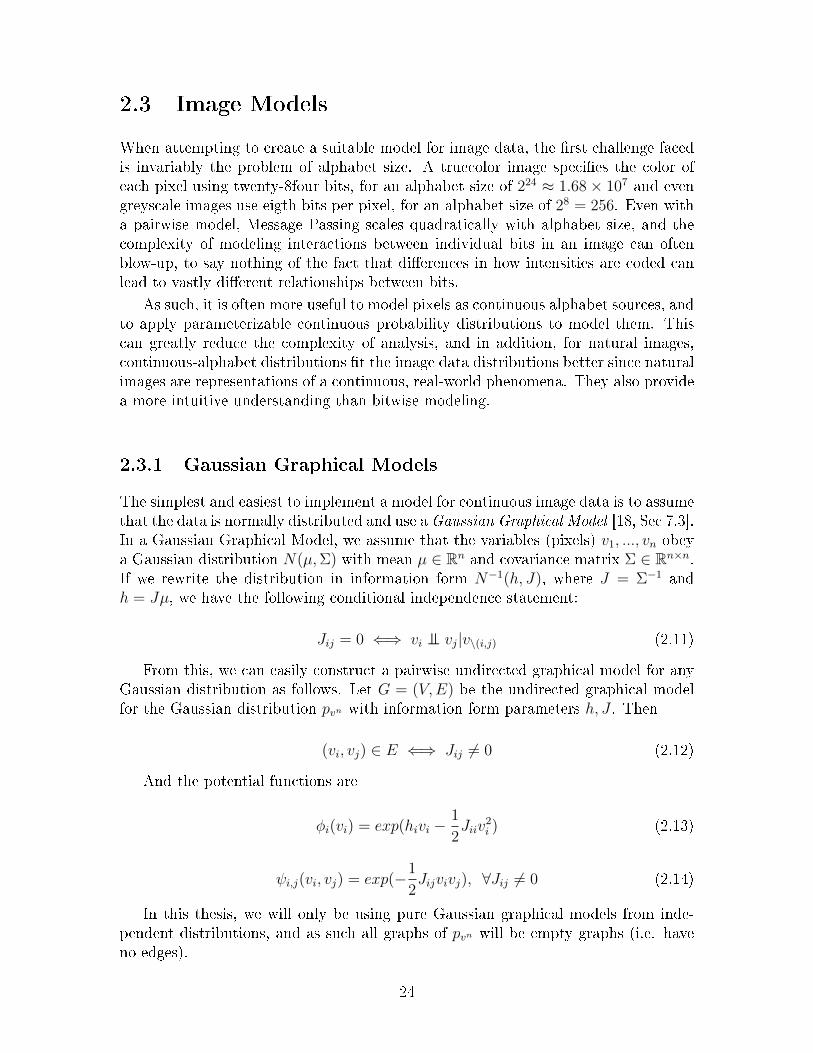
2-2 A pairwise graphical model representing a Gaussian distribution. . . . 25

2-3 A pairwise graphical model representing a Restricted Boltzmann Ma-chine. . . . . . . . . . . . . . . . . . . . . . . . . . . . . . . . . . . . 25

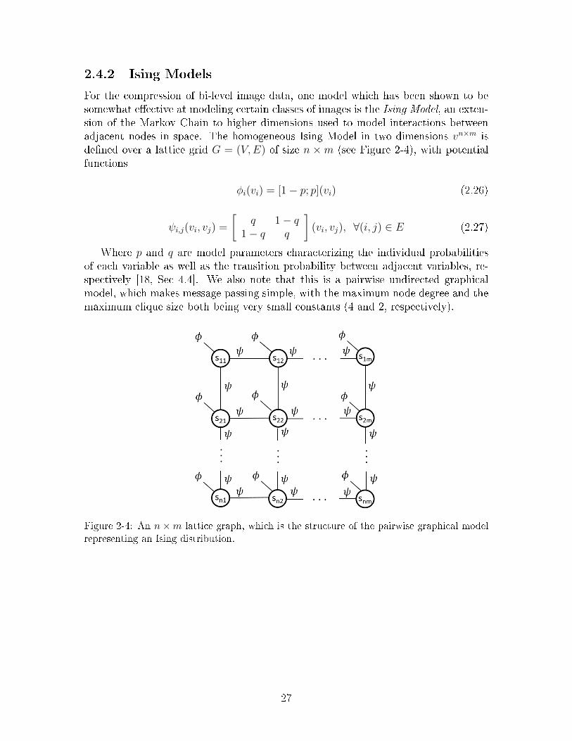
2-4 An 𝑛×𝑚 lattice graph, which is the structure of the pairwise graphicalmodel representing an Ising distribution. . . . . . . . . . . . . . . . . 27

3-1 The Model-Code-Separation graphical model for binary alphabet sourcesused by the decoder, containing both the source and code subgraphs . 30

3-2 The Model-Code-Separation graphical model for non-binary alphabetsources used by the decoder, containing both the source and code sub-graphs as well as the translation layer . . . . . . . . . . . . . . . . . . 32

3-3 The Model-Code-Quantizer-Separation graphical model with uniformquantization for continuous alphabet sources used by the decoder, con-taining both the source and code subgraphs as well as the translationand quantization layers . . . . . . . . . . . . . . . . . . . . . . . . . . 34

3-4 Plot of decoding errors as a function of compression rate illustratingthe three regimes of operation in a typical application of the MQCSsystem. . . . . . . . . . . . . . . . . . . . . . . . . . . . . . . . . . . . 36

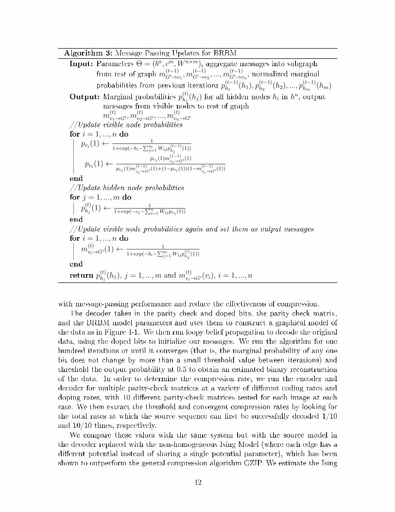
4-1 Decoding graph with BRBM source subgraph used for compressingMNIST database images. . . . . . . . . . . . . . . . . . . . . . . . . . 43

9

4-2 Threshold compression rate results of compressing 100 randomly se-lected images from the MNIST database using the separation archi-tecture under the Ising model and under the BRBM model with 2000hidden nodes with a dope rate of 0.05. The message-passing decoderwas run for a maximum of 100 iterations. Note that the BRBM modelalmost always provides better compression than the Ising model. . . . 44

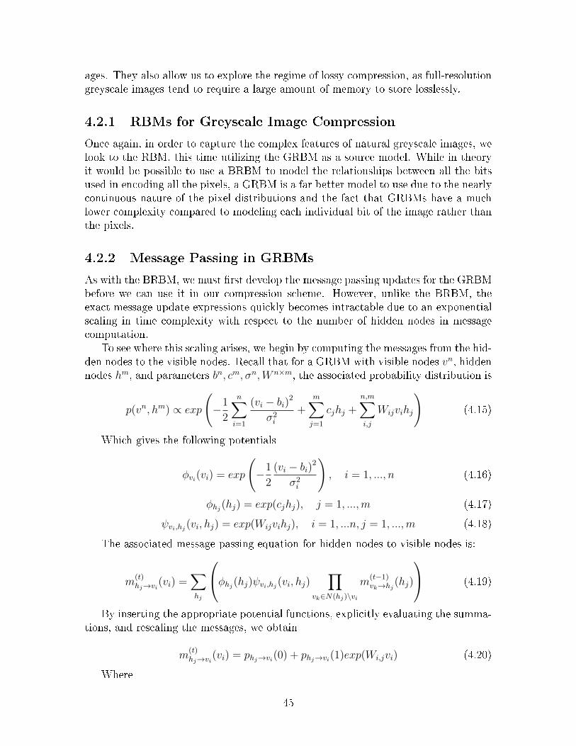
4-3 Threshold compression rate results (right) of compressing one ran-domly selected image from the MNIST database (left) under the BRBMmodel with varying number of hidden nodes with a dope rate of 0.05.The message-passing decoder was run for a maximum of 100 iterations.Note that the BRBM model performs better with more hidden nodesup until a saturation point. . . . . . . . . . . . . . . . . . . . . . . . 44

4-4 Sample images of the Cifar-10 image dataset. . . . . . . . . . . . . . . 484-5 Decoding graph with GRBM source subgraph used for compression of

Cifar-10 database images. . . . . . . . . . . . . . . . . . . . . . . . . 494-6 Average rate-distortion curve for the lossy compression of ten images

drawn randomly from the Cifar-10 database, compressed using theMQCS Architecture with a GRBM source model with 1500 nodes(RBM-1500), a GRBM source model with 500 nodes (RBM-500), aGRBM source model with 1500 nodes (RBM-1500), an independentGaussian source model (Indep), and compressed using the JPEG algo-rithm (JPEG). For the separation architecture, we allowed the message-passing algorithm to run up to 100 iterations for the decoder and usedan optimal dope rate of 1 bit per pixel. . . . . . . . . . . . . . . . . . 50

4-7 Five adjacent slices sampled from the X-ray tomography data used forthe 3D compression experiment. Note the strong continuity is the thirddimension. . . . . . . . . . . . . . . . . . . . . . . . . . . . . . . . . . 51

4-8 A 3 × 3 × 3 three-dimensional lattice graph (left) and three 3 × 3two-dimensional lattice graphs stacked on top of each other (right),which are examples of the two structures of the pairwise graphicalmodels representing their respective Ising distributions. Note that inthe stacked 2D case, each layer is independent of all other layers. . . . 52

10

List of Tables

1.1 Types of Data Compression Problems . . . . . . . . . . . . . . . . . . 14

4.1 Compression results for 60x60x40 3D tomography image. For theMQCS Architecture, threshold rates were used with a 0.125 dopingrate and a maximum of 300 message-passing iterations. . . . . . . . . 53

11

12

Chapter 1

Introduction

Data Compression is a long-studied problem of great importance, with applicationsin many fields. In recent years, developments in the field of machine learning has al-lowed for novel breakthroughs in solving this problem. One such breakthrough is thedevelopment of the Model-Quantizer-Code Separation (MQCS) Architecture for uni-versal compression. In this thesis, we extend the concept of the MQCS Architectureto the problem of lossy compression of continuous-alphabet sources and explore theapplications of this archiecture to the compression of images. We will also illustratethe benefits this architecture has over other methods of data compression.

1.1 Motivation

We begin with a motivating example to illustrate the necessity of the MQCS Archi-tecture.

1.1.1 Example: A Tale of Two Standards

In 1987, the Joint Photographic Experts Group (JPEG) released an image compres-sion standard for the lossless and lossy compression of natural images. The JPEGstandard used a perceptual model of image fidelity to design a quantization schemecentered around the discrete cosine transform (DCT) [33]. This standard soon becomethe most used method for compressing image data, used in most computer systemsas well as most digital cameras [31].

In 2000, the JPEG2000 standard was released by the same group [28]. The newstandard used an improved image model exploited by the wavelet transform to providecompression ratios and reconstruction fidelities superior to that of the original JPEGstandard as well as providing additional features such as scalability and progressivedecoding.

However, the standard format used for image compression in most modern com-puter systems is still JPEG, with few cameras even supporting JPEG2000 encod-ing, despite the improvements that JPEG2000 provides [1]. One main reason whyJPEG2000 never become a replacement for JPEG is the lack of backwards compati-

13

bility. JPEG and JPEG2000 use two completely different coding schemes, and as suchrequire two different encoders and decoders. Switching over to the JPEG2000 stan-dard would require re-encoding all existing JPEG images using the new codec and,in addition, most imaging software would need to continue to support both formatsfor a period of at least several years in the event that they encountered unconvertedfiles. In general, the benefits provided by JPEG2000 was not considered to be worththe trouble of switching over to the new system.

Since the creation of the JPEG standard, many advances have been made in thefield of image analysis and compression, and yet none of these advances have beenleveraged in modern computer systems, with JPEG remaining the standard. Thesame reasons that prevented the proliferation of JPEG2000 continues to make JPEGthe format of choices for image compression, as few wish to have to re-encode theirimages each time a better image model is developed.

1.1.2 A Universal Problem

The phenomenon observed in the history of image compression is not an isolatedincident. In many applications where data must be compressed without a completeknowledge of the source from which the data is drawn from, it is difficult to leverageadditional knowledge discovered about the source model ex post facto. Attempts todo so either lead to the creation of new standards which are only adapted by a smallnumber of users, or which clutter decoding programs that need to be backwards-compatible with multiple formats.

1.1.3 Types of Compression and Joint Design

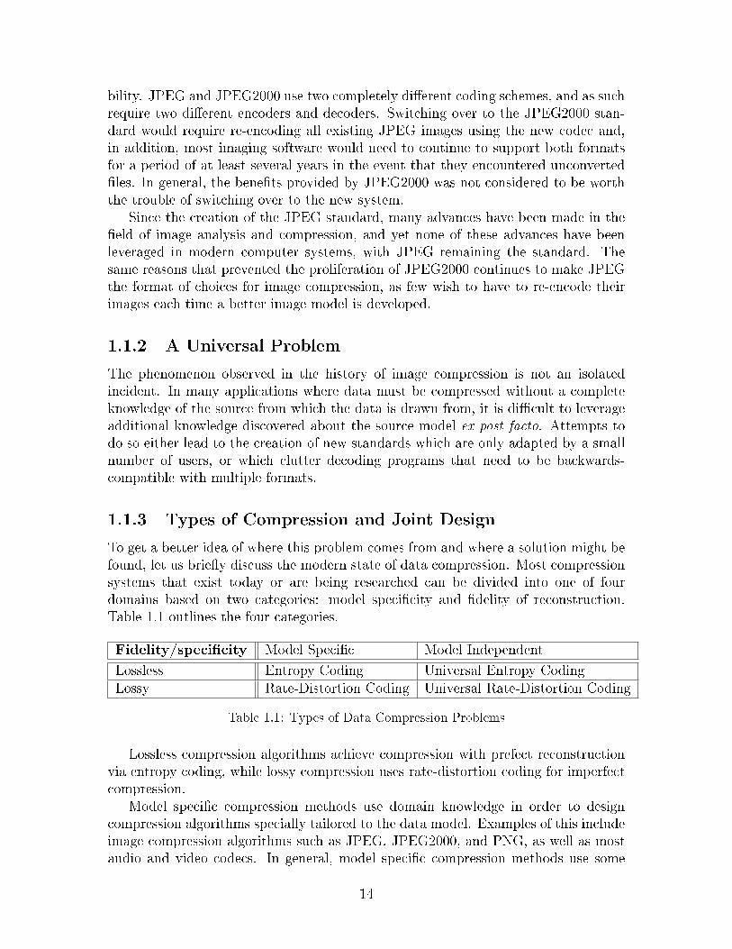
To get a better idea of where this problem comes from and where a solution might befound, let us briefly discuss the modern state of data compression. Most compressionsystems that exist today or are being researched can be divided into one of fourdomains based on two categories: model specificity and fidelity of reconstruction.Table 1.1 outlines the four categories.

Fidelity/specificity Model Specific Model Independent

Lossless Entropy Coding Universal Entropy CodingLossy Rate-Distortion Coding Universal Rate-Distortion Coding

Table 1.1: Types of Data Compression Problems

Lossless compression algorithms achieve compression with prefect reconstructionvia entropy coding, while lossy compression uses rate-distortion coding for imperfectcompression.

Model specific compression methods use domain knowledge in order to designcompression algorithms specially tailored to the data model. Examples of this includeimage compression algorithms such as JPEG, JPEG2000, and PNG, as well as mostaudio and video codecs. In general, model specific compression methods use some

14

form of data processing followed by an entropy coding step (e.g. Huffman coding,arithmetic coding), with an additional quantization step for lossy compression thatare often integrated with the coding and processing steps. (e.g. EZW coding, Lloyd-max quantization).

Model independent (universal) coding does not require any prior knowledge aboutthe source of the data being compressed, instead relying on universal methods ofentropy coding (e.g. LZW coding, CTW coding).

Both model specific and model independent compression have their advantagesand disadvantages. Model specific compression is, in general, very effective at com-pressing the type of data it is designed to compressed, and uses domain knowledgeto greatly improve compression performance. However, model specific compressionis hampered by the concept of joint design, where the data-processing, quantization,and coding steps must be designed jointly for maximum performance based on thesource model. Figure 1-1 illustrates the concept of joint design.

Figure 1-1: The joint design paradigm, where the data model is required in the construction

of the encoder, and the processing, quantization, and coding steps are intertwined.

We can see this paradigm in action in JPEG coding, where the pre-processingstep of transforming the data into the DCT domain is done because it can be coupledwith a quantization procedure based on perceptual models of vision, which allowsfor effective run-length coding, which in turn can be effectively compressed usingHuffman coding. Each part of the system is effective only because the other partsof the system are designed to work specifically with it and the overall source model.This makes the system rigid and makes is often impossible or very difficult to includenew domain knowledge into an existing system. In addition, to design model-specificsystems, one must already possess the domain knowledge, which means that the datacannot be encoded until enough data has been collected to understand the sourcemodel, which is not always optimal.

Model independent coding avoids these issues by using a universal code, whichallows for the encoding of data without any prior knowledge of the source. However,universal codes are unable to leverage knowledge of the source model, and for complexmodels, require very long bitstreams to achieve effective compression.

Ideally, we would like to be able to leverage the benefits of both types of coding. Towit, we would like a universal encoding system that allows for data to be compressedwithout knowledge of the source model, and would also like a system that is ableto integrate varying amounts of domain knowledge in order to improve compression

15

performance.

1.1.4 Image Compression

One particular domain where this type of universal coding would be useful is inthe compression of images. Image data tends to be highly structured in complex,non-linear ways and, given the ubiquity of this type of data and its importance inmany applications, work is constantly being done to improve our ability to analyzeand model images. As discussed in the motivating example, however, much of thiswork has not be used to benefit image compression systems, with JPEG continuingto dominate decades after its release despite all the advances in the field. With auniversal, easily-upgradable system, it would be possible to finally create an imagecompression algorithm that can leverage current advances in imaging as well as futuredevelopments without sacrificing backwards-compatibility.

1.2 Previous Work

1.2.1 The Model-Quantizer-Code Separation Architecture

The problem of eliminating joint design from compression architectures was studiedin-depth by Huang and Wornell [17] [16] and later by Lai [21]. Huang and Wornellproposed a source-agnostic universal data compression architecture known as theModel-Quantizer-Code Separation (MQCS) Architecture.

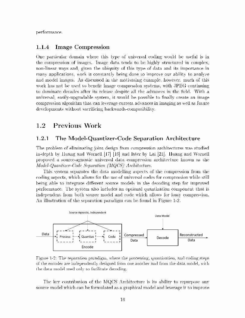
This system separates the data modelling aspects of the compression from thecoding aspects, which allows for the use of universal codes for compression while stillbeing able to integrate different source models in the decoding step for improvedperformance. The system also includes an optional quantization component that isindependent from both source model and code which allows for lossy compression.An illustration of the separation paradigm can be found in Figure 1-2.

Figure 1-2: The separation paradigm, where the processing, quantization, and coding steps

of the encoder are independently designed from one another and from the data model, with

the data model used only to facilitate decoding.

The key contribution of the MQCS Architecture is its ability to repurpose anysource model which can be formulated as a graphical model and leverage it to improve

16

decoding performance and thus compression performance. A more detailed outline ofthe functionality of the MQCS Architecture will be given in Chapter 3.

1.2.2 Image Modeling

All image compression algorithms rely on some underlying model of how the imageis generated. In this thesis, we focus on natural images; that is, pictures from thereal world, which is the same subset that most image compression systems focus on,including JPEG and JPEG2000. Over the course of the past thirty years, manyadvances have been made in this regard.

The original JPEG standard used an image model whereby low-frequency com-ponents of the Discrete Cosine Transform (DCT) of the image were more significantthan the high-frequency components [33]. The JPEG2000 standard refined this modelwith the wavelet transform, allowing some important high-frequency components tobe conserved as well [28]. Later models were then developed, though never leveragedfor practical image compression applications.

Gaussian and Laplacian image pyramids provide simple hierarchal methods for de-composing an image into component parts, allowing for image analysis and processingat multiple resolution levels [5]. Later, Restricted Boltzmann Machines (RBMs) weredeveloped to model images using mixture models and perform feature detection onthem [22]. More recently, significant work has been done in the field of deep learningwith regard to the classification and generation of images [7] [27].

Deep Neural Networks have been used extensively for image classification [6], andthe idea of stacking multiple layers of nodes have been extended to RBMs to createDeep Belief Networks, which consist of stacks of RBMs [13]. Finally, to providescalability of these systems, convolutional networks have been developed for bothDeep Neural Nets [20] and Deep Belief Nets [24], enforcing certain patterns in theconnections between layers to reduce complexity.

1.3 Contributions

In this thesis, we extend the work done by Huang and Wornell and Lai in the de-velopment of the MQCS Architecture into practical applications of compression ofcontinuous or large-cardinality alphabet sources. Specifically, we will look at thecompression of natural image data. We will show how the MQCS Architecture canbe used to compress image data using different source models for both bi-level andgreyscale images.

We will begin by modeling the pixels of the image as being drawn from a Gaussianor Gaussian mixture distribution and explore different methods for determining thisdistribution and how the resulting model can be used in the MQCS Architecture.In particular, we will focus on the Restricted Boltzmann Machine and its variations,showing how these models can connected to the MQCS Architecture and derivingapproximate expressions for message-passing in these models. Finally, we will explorethe model-adaptive potential of the MQCS Architecture by looking at the compression

17

of 2D and 3D bi-level image data and showing how the MQCS Architecture can bequickly modified with new source models to improve compression performance.

1.4 Thesis Organization

This thesis will cover both the overall design of the MQCS Architecture as well as itsimplementations on real-world data. In particular, the organization of the thesis willbe as follows:

Chapter 2 will provide a brief overview of various basic concepts that serve as thebasis of the MQCS Architecture, as well as an overview of the image models that willbe used in the thesis. Chapter 3 will provide a description of the MQCS Architecture,including its use as an encoder or decoder for various types of data and how to leverageinformation about source models to improve compression performance via graphicalmodeling. Chapter 4 will explore the applications of the MQCS Architecture tothe problem of image compression, including discussions of the results of experimentsperformed on various datasets. Finally, Chapter 5 will conclude the thesis and discusspotential for future work that can be done with the MQCS Architecture.

1.5 Notation

While we have endeavored to use the standard notations and terminology, the multi-disciplinary nature of the system coupled with the fact that some of the fields inquestion are quite new and developing quickly mean that there will often be multiplecompeting or contradicting sets of notation that we will encounter. As such, thefollowing list outlines the notation we have chosen for this thesis unless otherwisenoted.

∙ We use lower case 𝑠 to denote a scalar or vector variable. For a vector variable,we denote the length using superscripts (e.g. 𝑠𝑛) when introducing the variable,with subscript indexing (e.g. 𝑠𝑛𝑖 is the 𝑖th element of 𝑠𝑛). We also use thebackslash to indicate all other elements in a vector (e.g. 𝑠∖(𝑖,𝑗) are all elementsin 𝑠𝑛 except for the 𝑖th and 𝑗th element).

∙ We use upper case 𝐴 to denote a matrix, with size specified by superscripts𝐴𝑛×𝑚 and indexing done using subscripts (e.g. 𝐴𝑖𝑗 is the (𝑖, 𝑗)th entry of 𝐴).

∙ For iterative algorithms, we use bracketed superscripts to denote iteration num-ber (𝑚(𝜏) is the value of 𝑚 at the 𝜏th iteration).

∙ We use R to denote the set of real numbers and Z𝑝 to denote the set of integers𝑚𝑜𝑑 𝑝.

∙ For algorithms, we use doubles slashes // to indicate the beginning of a com-ment.

∙ We use 1{𝑥} to denote the indicator function, which evaluates to 1 if the state-ment 𝑥 is true, and zero otherwise. We also use 𝑒𝑥𝑝(𝑥) to denote the exponentialfunction 𝑒𝑥.

18

Chapter 2

Background

The development and implementation of the MQCS Architecture is an undertakingthat spans multiple fields of study. The fundamental concepts behind the quanti-zation and compression of data come from the field of information theory, with theactual codes used coming from coding theory. The developments of the decoder anddecoding algorithms are drawn from the field of inference and probabilistic model-ing. And finally, the models used for compression are mainly drawn from the field ofmachine learning. In this chapter, we will provide an overview of the key conceptsneeded for the understanding of the MQCS Architecture, including relevant defini-tions and results. Chapter 3 will expand on this background, showing how all thepieces discussed can be put together to form the compression architecture.

2.1 Probabilistic Graphical Models

Probabilistic Graphical Models (PGMs) are powerful tools used to model conditionaldependencies between variables in a probabilistic distribution. A PGM representsa distribution as a graph, with nodes representing variables and edges representingrelations between variables. There are a few types of graphical models, but in thisthesis the focus shall be on undirected graphical models and factor graphs.

2.1.1 Undirected Graphical Models

An undirected graphical model is an undirected graph 𝐺 = (𝑉,𝐸) in which each node𝑣𝑖 ∈ 𝑉 represents a variable, and each edge (𝑣𝑖, 𝑣𝑗) ∈ 𝐸 represents a conditionaldependency. That is, for any two variables:

(𝑣𝑖, 𝑣𝑗) /∈ 𝐸 =⇒ 𝑣𝑖 á 𝑣𝑗|𝑣∖(𝑖,𝑗) (2.1)

By the Hammersley-Clifford theorem [18, Thm 4.2], any strictly positive prob-ability distribution can be represented using this form, and the probability densityfunction can be factored out into a product of functions over the cliques of the graph.

19

𝑝(𝑣) ∝∏𝐶∈𝒞

𝜓𝐶(𝑣𝐶) (2.2)

Where 𝜓𝐶(𝑣𝐶) is the potential function of clique 𝐶 and 𝒞 is the set of all cliquesin 𝐺.

One useful subset of undirected graphical models are pairwise graphical models. Ina pairwise graphical model, the largest clique size is two, and as such the probabilitydensity function can be factored into a product of functions of two nodes:

𝑝(𝑣) ∝∏

(𝑖,𝑗)∈𝐸

𝜓𝑖,𝑗(𝑣𝑖, 𝑣𝑗) (2.3)

Pairwise models are especially attractive due to their simplicity and the easein which inference can be performed over them, as well as the fact that each edgerepresents a distinct potential function.

2.1.2 Factor Graphs

In addition to undirected graphical models, another PGM of interest is the FactorGraph (FG) [18, Sec 4.4]. A factor graph is a bipartite graph 𝐺 = (𝑉, 𝐹,𝐸) with twosets of nodes. Variable nodes 𝑣1, ..., 𝑣𝑁 ∈ 𝑉 represent variables in the distributionand factor nodes 𝑓1, ..., 𝑓𝑀 ∈ 𝐹 represent functions. The probability density functionof the distribution represented by a factor graph is given by:

𝑝(𝑣) ∝𝑀∏𝑖=1

𝑓𝑖(𝑣𝑁(𝑓𝑖)) (2.4)

Where 𝑁(𝑓𝑖) is the neighborhood of 𝑓𝑖 or the set of variable nodes adjacent to 𝑓𝑖.Both undirected graphical models and factor graphs are useful tools for represent-

ing probability distributions, and both will be used in this thesis.

2.1.3 Inference in PGMs: Belief Propagation and Loopy Belief

Propagation

Once a model for the probability distribution has been determined, the next step isto perform inference over the model to extract the necessary information from it. Inthis case, our goal is to determine the marginal distribution of a variable or multiplevariables. In the case where the variables are drawn from a discrete alphabet source,marginalization can be computed using a brute-force method by summing over allvariables except for the variable being isolated:

𝑝(𝑣𝑖) =∑𝑣∖𝑖

𝑝(𝑣1, ..., 𝑣𝑁) (2.5)

For continuous alphabets, the summation would be replaced by integration overthe variables. Direct computation of this marginal is exponential in the number of

20

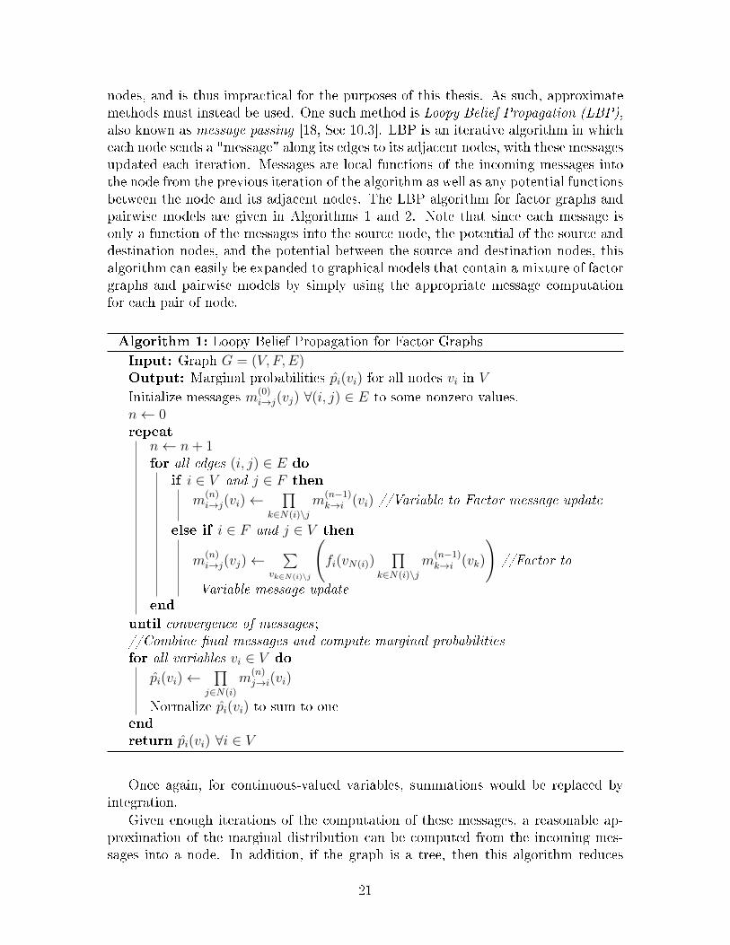
nodes, and is thus impractical for the purposes of this thesis. As such, approximatemethods must instead be used. One such method is Loopy Belief Propagation (LBP),also known as message passing [18, Sec 10.3]. LBP is an iterative algorithm in whicheach node sends a "message" along its edges to its adjacent nodes, with these messagesupdated each iteration. Messages are local functions of the incoming messages intothe node from the previous iteration of the algorithm as well as any potential functionsbetween the node and its adjacent nodes. The LBP algorithm for factor graphs andpairwise models are given in Algorithms 1 and 2. Note that since each message isonly a function of the messages into the source node, the potential of the source anddestination nodes, and the potential between the source and destination nodes, thisalgorithm can easily be expanded to graphical models that contain a mixture of factorgraphs and pairwise models by simply using the appropriate message computationfor each pair of node.

Algorithm 1: Loopy Belief Propagation for Factor Graphs

Input: Graph 𝐺 = (𝑉, 𝐹,𝐸)Output: Marginal probabilities 𝑝𝑖(𝑣𝑖) for all nodes 𝑣𝑖 in 𝑉

Initialize messages 𝑚(0)𝑖→𝑗(𝑣𝑗) ∀(𝑖, 𝑗) ∈ 𝐸 to some nonzero values.

𝑛← 0repeat

𝑛← 𝑛+ 1for all edges (𝑖, 𝑗) ∈ 𝐸 do

if 𝑖 ∈ 𝑉 and 𝑗 ∈ 𝐹 then

𝑚(𝑛)𝑖→𝑗(𝑣𝑖)←

∏𝑘∈𝑁(𝑖)∖𝑗

𝑚(𝑛−1)𝑘→𝑖 (𝑣𝑖) //Variable to Factor message update

else if 𝑖 ∈ 𝐹 and 𝑗 ∈ 𝑉 then

𝑚(𝑛)𝑖→𝑗(𝑣𝑗)←

∑𝑣𝑘∈𝑁(𝑖)∖𝑗

(𝑓𝑖(𝑣𝑁(𝑖))

∏𝑘∈𝑁(𝑖)∖𝑗

𝑚(𝑛−1)𝑘→𝑖 (𝑣𝑘)

)//Factor to

Variable message updateend

until convergence of messages ;//Combine final messages and compute marginal probabilitiesfor all variables 𝑣𝑖 ∈ 𝑉 do

𝑝𝑖(𝑣𝑖)←∏

𝑗∈𝑁(𝑖)

𝑚(𝑛)𝑗→𝑖(𝑣𝑖)

Normalize 𝑝𝑖(𝑣𝑖) to sum to oneendreturn 𝑝𝑖(𝑣𝑖) ∀𝑖 ∈ 𝑉

Once again, for continuous-valued variables, summations would be replaced byintegration.

Given enough iterations of the computation of these messages, a reasonable ap-proximation of the marginal distribution can be computed from the incoming mes-sages into a node. In addition, if the graph is a tree, then this algorithm reduces

21

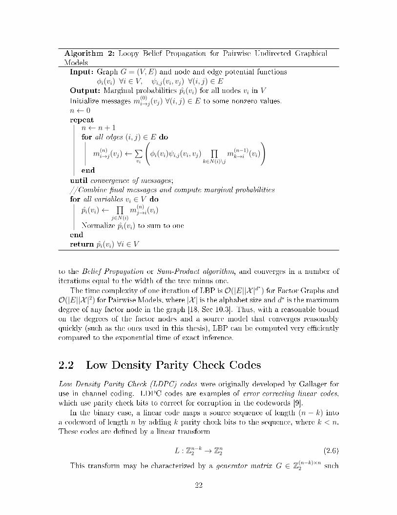
Algorithm 2: Loopy Belief Propagation for Pairwise Undirected GraphicalModelsInput: Graph 𝐺 = (𝑉,𝐸) and node and edge potential functions

𝜑𝑖(𝑣𝑖) ∀𝑖 ∈ 𝑉, 𝜓𝑖,𝑗(𝑣𝑖, 𝑣𝑗) ∀(𝑖, 𝑗) ∈ 𝐸Output: Marginal probabilities 𝑝𝑖(𝑣𝑖) for all nodes 𝑣𝑖 in 𝑉

Initialize messages 𝑚(0)𝑖→𝑗(𝑣𝑗) ∀(𝑖, 𝑗) ∈ 𝐸 to some nonzero values.

𝑛← 0repeat

𝑛← 𝑛+ 1for all edges (𝑖, 𝑗) ∈ 𝐸 do

𝑚(𝑛)𝑖→𝑗(𝑣𝑗)←

∑𝑣𝑖

(𝜑𝑖(𝑣𝑖)𝜓𝑖,𝑗(𝑣𝑖, 𝑣𝑗)

∏𝑘∈𝑁(𝑖)∖𝑗

𝑚(𝑛−1)𝑘→𝑖 (𝑣𝑖)

)end

until convergence of messages ;//Combine final messages and compute marginal probabilitiesfor all variables 𝑣𝑖 ∈ 𝑉 do

𝑝𝑖(𝑣𝑖)←∏

𝑗∈𝑁(𝑖)

𝑚(𝑛)𝑗→𝑖(𝑣𝑖)

Normalize 𝑝𝑖(𝑣𝑖) to sum to oneendreturn 𝑝𝑖(𝑣𝑖) ∀𝑖 ∈ 𝑉

to the Belief Propagation or Sum-Product algorithm, and converges in a number ofiterations equal to the width of the tree minus one.

The time complexity of one iteration of LBP is 𝒪(|𝐸||𝒳 |𝑑*) for Factor Graphs and𝒪(|𝐸||𝒳 |2) for Pairwise Models, where |𝒳 | is the alphabet size and 𝑑* is the maximumdegree of any factor node in the graph [18, Sec 10.3]. Thus, with a reasonable boundon the degrees of the factor nodes and a source model that converges reasonablyquickly (such as the ones used in this thesis), LBP can be computed very efficientlycompared to the exponential time of exact inference.

2.2 Low Density Parity Check Codes

Low Density Parity Check (LDPC) codes were originally developed by Gallager foruse in channel coding. LDPC codes are examples of error-correcting linear codes,which use parity check bits to correct for corruption in the codewords [9].

In the binary case, a linear code maps a source sequence of length (𝑛 − 𝑘) intoa codeword of length 𝑛 by adding 𝑘 parity check bits to the sequence, where 𝑘 < 𝑛.These codes are defined by a linear transform

𝐿 : Z𝑛−𝑘2 → Z𝑛

2 (2.6)

This transform may be characterized by a generator matrix 𝐺 ∈ Z(𝑛−𝑘)×𝑛2 such

22

that

𝐿(𝑠) = 𝐺𝑇 𝑠 (2.7)

An equivalent characterization is the parity-check matrix 𝐻 ∈ Z𝑘×𝑛2 satisfying

𝐻𝐺𝑇 = 0 (2.8)

From which the parity-check bits 𝑥𝑘 can be computed from the codeword 𝑠𝑛 by

𝑥 = 𝐻𝑠 (2.9)

LDPC codes are linear codes with sparse parity check matrices 𝐻, that is, therow and column weights of 𝐻 are negligible as 𝑛 grows to infinity. LDPC codes havebeen shown to approach capacity and are thus popular for use in channel coding [15].

2.2.1 Modeling LDPC Codes

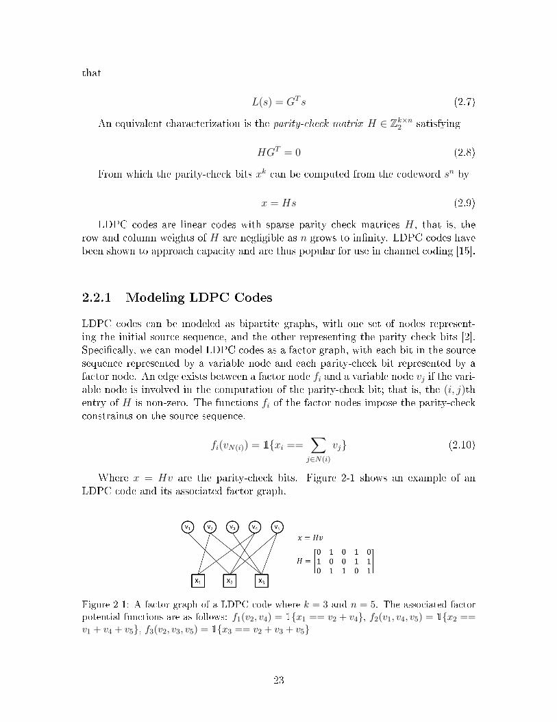
LDPC codes can be modeled as bipartite graphs, with one set of nodes represent-ing the initial source sequence, and the other representing the parity check bits [2].Specifically, we can model LDPC codes as a factor graph, with each bit in the sourcesequence represented by a variable node and each parity-check bit represented by afactor node. An edge exists between a factor node 𝑓𝑖 and a variable node 𝑣𝑗 if the vari-able node is involved in the computation of the parity-check bit; that is, the (𝑖, 𝑗)thentry of 𝐻 is non-zero. The functions 𝑓𝑖 of the factor nodes impose the parity-checkconstraints on the source sequence.

𝑓𝑖(𝑣𝑁(𝑖)) = 1{𝑥𝑖 ==∑

𝑗∈𝑁(𝑖)

𝑣𝑗} (2.10)

Where 𝑥 = 𝐻𝑣 are the parity-check bits. Figure 2-1 shows an example of anLDPC code and its associated factor graph.

Figure 2-1: A factor graph of a LDPC code where 𝑘 = 3 and 𝑛 = 5. The associated factor

potential functions are as follows: 𝑓1(𝑣2, 𝑣4) = 1{𝑥1 == 𝑣2 + 𝑣4}, 𝑓2(𝑣1, 𝑣4, 𝑣5) = 1{𝑥2 ==𝑣1 + 𝑣4 + 𝑣5}, 𝑓3(𝑣2, 𝑣3, 𝑣5) = 1{𝑥3 == 𝑣2 + 𝑣3 + 𝑣5}

23

2.3 Image Models

When attempting to create a suitable model for image data, the first challenge facedis invariably the problem of alphabet size. A truecolor image specifies the color ofeach pixel using twenty-8four bits, for an alphabet size of 224 ≈ 1.68× 107 and evengreyscale images use eigth bits per pixel, for an alphabet size of 28 = 256. Even witha pairwise model, Message Passing scales quadratically with alphabet size, and thecomplexity of modeling interactions between individual bits in an image can oftenblow-up, to say nothing of the fact that differences in how intensities are coded canlead to vastly different relationships between bits.

As such, it is often more useful to model pixels as continuous alphabet sources, andto apply parameterizable continuous probability distributions to model them. Thiscan greatly reduce the complexity of analysis, and in addition, for natural images,continuous-alphabet distributions fit the image data distributions better since naturalimages are representations of a continuous, real-world phenomena. They also providea more intuitive understanding than bitwise modeling.

2.3.1 Gaussian Graphical Models

The simplest and easiest to implement a model for continuous image data is to assumethat the data is normally distributed and use aGaussian Graphical Model [18, Sec 7.3].In a Gaussian Graphical Model, we assume that the variables (pixels) 𝑣1, ..., 𝑣𝑛 obeya Gaussian distribution 𝑁(𝜇,Σ) with mean 𝜇 ∈ R𝑛 and covariance matrix Σ ∈ R𝑛×𝑛.If we rewrite the distribution in information form 𝑁−1(ℎ, 𝐽), where 𝐽 = Σ−1 andℎ = 𝐽𝜇, we have the following conditional independence statement:

𝐽𝑖𝑗 = 0 ⇐⇒ 𝑣𝑖 á 𝑣𝑗|𝑣∖(𝑖,𝑗) (2.11)

From this, we can easily construct a pairwise undirected graphical model for anyGaussian distribution as follows. Let 𝐺 = (𝑉,𝐸) be the undirected graphical modelfor the Gaussian distribution 𝑝𝑣𝑛 with information form parameters ℎ, 𝐽 . Then

(𝑣𝑖, 𝑣𝑗) ∈ 𝐸 ⇐⇒ 𝐽𝑖𝑗 = 0 (2.12)

And the potential functions are

𝜑𝑖(𝑣𝑖) = 𝑒𝑥𝑝(ℎ𝑖𝑣𝑖 −1

2𝐽𝑖𝑖𝑣

2𝑖 ) (2.13)

𝜓𝑖,𝑗(𝑣𝑖, 𝑣𝑗) = 𝑒𝑥𝑝(−1

2𝐽𝑖𝑗𝑣𝑖𝑣𝑗), ∀𝐽𝑖𝑗 = 0 (2.14)

In this thesis, we will only be using pure Gaussian graphical models from inde-pendent distributions, and as such all graphs of 𝑝𝑣𝑛 will be empty graphs (i.e. haveno edges).

24

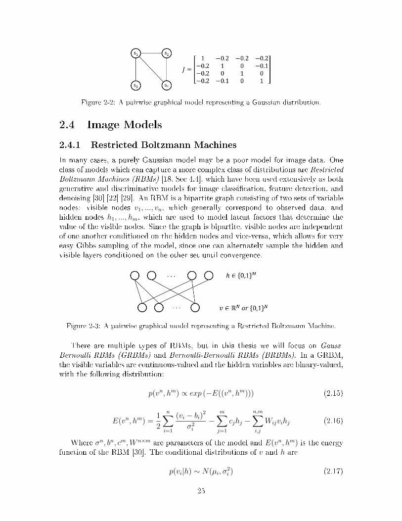
Figure 2-2: A pairwise graphical model representing a Gaussian distribution.

2.4 Image Models

2.4.1 Restricted Boltzmann Machines

In many cases, a purely Gaussian model may be a poor model for image data. Oneclass of models which can capture a more complex class of distributions are RestrictedBoltzmann Machines (RBMs) [18, Sec 4.4], which have been used extensively as bothgenerative and discriminative models for image classification, feature detection, anddenoising [30] [22] [29]. An RBM is a bipartite graph consisting of two sets of variablenodes: visible nodes 𝑣1, ..., 𝑣𝑛, which generally correspond to observed data, andhidden nodes ℎ1, ..., ℎ𝑚, which are used to model latent factors that determine thevalue of the visible nodes. Since the graph is bipartite, visible nodes are independentof one another conditioned on the hidden nodes and vice-versa, which allows for veryeasy Gibbs sampling of the model, since one can alternately sample the hidden andvisible layers conditioned on the other set until convergence.

Figure 2-3: A pairwise graphical model representing a Restricted Boltzmann Machine.

There are multiple types of RBMs, but in this thesis we will focus on Gauss-Bernoulli RBMs (GRBMs) and Bernoulli-Bernoulli RBMs (BRBMs). In a GRBM,the visible variables are continuous-valued and the hidden variables are binary-valued,with the following distribution:

𝑝(𝑣𝑛, ℎ𝑚) ∝ 𝑒𝑥𝑝 (−𝐸((𝑣𝑛, ℎ𝑚))) (2.15)

𝐸(𝑣𝑛, ℎ𝑚) =1

2

𝑛∑𝑖=1

(𝑣𝑖 − 𝑏𝑖)2

𝜎2𝑖

−𝑚∑𝑗=1

𝑐𝑗ℎ𝑗 −𝑛,𝑚∑𝑖,𝑗

𝑊𝑖𝑗𝑣𝑖ℎ𝑗 (2.16)

Where 𝜎𝑛, 𝑏𝑛, 𝑐𝑚,𝑊 𝑛×𝑚 are parameters of the model and 𝐸(𝑣𝑛, ℎ𝑚) is the energyfunction of the RBM [30]. The conditional distributions of 𝑣 and ℎ are

𝑝(𝑣𝑖|ℎ) ∼ 𝑁(𝜇𝑖, 𝜎2𝑖 ) (2.17)

25

𝜇𝑖 = 𝑏𝑖 + 𝜎2𝑖

∑𝑗

𝑊𝑖𝑗ℎ𝑗 (2.18)

𝑝(ℎ𝑗 = 1|𝑣) =1

1 + 𝑒𝑥𝑝 (−∑

𝑖𝑊𝑖𝑗𝑣𝑖 − 𝑐𝑗)(2.19)

That is, the GRBM models a Gaussian Mixture Model with parameters definedby the GRBM parameters and each configuration of hidden nodes creating a differentGaussian distribution.

In a BRBM, the visible variables and the hidden variables are binary-valued, withthe following distribution:

𝑝(𝑣𝑛, ℎ𝑚) ∝ 𝑒𝑥𝑝 (−𝐸((𝑣𝑛, ℎ𝑚))) (2.20)

𝐸(𝑣𝑛, ℎ𝑚) = −𝑛∑

𝑖=1

𝑏𝑖𝑣𝑖 −𝑚∑𝑗=1

𝑐𝑗ℎ𝑗 −𝑛,𝑚∑𝑖,𝑗

𝑊𝑖𝑗𝑣𝑖ℎ𝑗 (2.21)

Where 𝑏𝑛, 𝑐𝑚,𝑊 𝑛×𝑚 are parameters of the model. The conditional distributionsof 𝑣 and ℎ are

𝑝(𝑣𝑖 = 1|ℎ) =1

1 + 𝑒𝑥𝑝(−∑

𝑗 𝑊𝑖𝑗ℎ𝑗 − 𝑏𝑖) (2.22)

𝑝(ℎ𝑗 = 1|𝑣) =1

1 + 𝑒𝑥𝑝 (−∑

𝑖𝑊𝑖𝑗𝑣𝑖 − 𝑐𝑗)(2.23)

In this case, hidden variables can be used to model underlying features that affectthe values of the visible variables [30].

For both types of models, the standard method for training RBMs is to use agradient descent method. The update rules for the parameter set Θ = (𝑏𝑛, 𝑐𝑚,𝑊 𝑛×𝑚)is

Θ(𝑡) = Θ(𝑡−1) + 𝜂𝑑𝐿(Θ; 𝑣)

𝑑Θ

Θ(𝑡−1)

(2.24)

Where 𝜂 is the learning rate and 𝐿(Θ; 𝑣) is the average log-likelihood of the data𝑣 and the parameters Θ. Using the Constrastive Divergence technique, we have that

𝑑𝐿(Θ; 𝑣)

𝑑Θ= −E𝑑𝑎𝑡𝑎(𝐸(𝑣, ℎ, ; Θ)) + E𝑚𝑜𝑑𝑒𝑙(𝐸(𝑣, ℎ; Θ)) (2.25)

E𝑑𝑎𝑡𝑎(·) is the expectation of the data over the model, which can be evaluatedby taking an empirical average of the energy function over all the training data, andE𝑚𝑜𝑑𝑒𝑙(·) is the expectation over the model, which can be calculated by performingGibbs sampling on the RBM a finite number of times to produce an "average" re-alization of the data and then evaluating the expression using that realization [12].This algorithm can be used to train both BRBMs and GRBMs by using the correctenergy functions and parameter sets.

26

2.4.2 Ising Models

For the compression of bi-level image data, one model which has been shown to besomewhat effective at modeling certain classes of images is the Ising Model, an exten-sion of the Markov Chain to higher dimensions used to model interactions betweenadjacent nodes in space. The homogeneous Ising Model in two dimensions 𝑣𝑛×𝑚 isdefined over a lattice grid 𝐺 = (𝑉,𝐸) of size 𝑛 ×𝑚 (see Figure 2-4), with potentialfunctions

𝜑𝑖(𝑣𝑖) = [1− 𝑝; 𝑝](𝑣𝑖) (2.26)

𝜓𝑖,𝑗(𝑣𝑖, 𝑣𝑗) =

[𝑞 1− 𝑞

1− 𝑞 𝑞

](𝑣𝑖, 𝑣𝑗), ∀(𝑖, 𝑗) ∈ 𝐸 (2.27)

Where 𝑝 and 𝑞 are model parameters characterizing the individual probabilitiesof each variable as well as the transition probability between adjacent variables, re-spectively [18, Sec 4.4]. We also note that this is a pairwise undirected graphicalmodel, which makes message passing simple, with the maximum node degree and themaximum clique size both being very small constants (4 and 2, respectively).

Figure 2-4: An 𝑛×𝑚 lattice graph, which is the structure of the pairwise graphical model

representing an Ising distribution.

27

28

Chapter 3

The Model-Quantizer-Code

Separation Architecture

Equipped with the fundamental concepts underlying the MQCS Architecture, we arenow prepared to describe its operation. Since the MQCS Architecture is modular,this chapter will show its full construction component by component, from a simplelossless binary compressor to a complete architecture which can be used to compressalmost any type of data.

3.1 The Binary Lossless Model-Code Separation Ar-

chitecture

We begin by looking at the problem of losslessly compressing a stream of binary digits.Without any prior knowledge of where this data stream comes from, we cannot designa specific compression scheme for it, and must thus default to using universal codessuch as LZW coding, which is guaranteed to eventually reach entropy but may requireunrealistically long bitstreams before achieving a compression rate close to the bestpossible rate. On the other hand, if we know the source of the data, we can usemore efficient coding techniques such as Huffman Coding. However, for most of thesetechniques, if more information is ever gained about the source, the entire compressionsystem must be redesigned from scratch.

To solve this issue of flexibility, the Model-Code Separation (MCS) architectureuses LDPC codes for universal compression, followed by Message Passing for decoding.Specifically, the encoder and decoder are designed as follows.

The encoder requires an input sequence 𝑠𝑛 ∈ Z𝑛2 to compress and a randomly-

generated parity-check matrix 𝐻 ∈ Z𝑘×𝑛2 . The output of the encoder are the parity-

check bits:

𝑥𝑘 = 𝐻𝑠𝑛 (3.1)

𝑥𝑘 comprises the compressed output of the encoder. Thus, we see that the encodercompresses 𝑛 bits to 𝑘 bits, for a compression rate of 𝑘/𝑛.

29

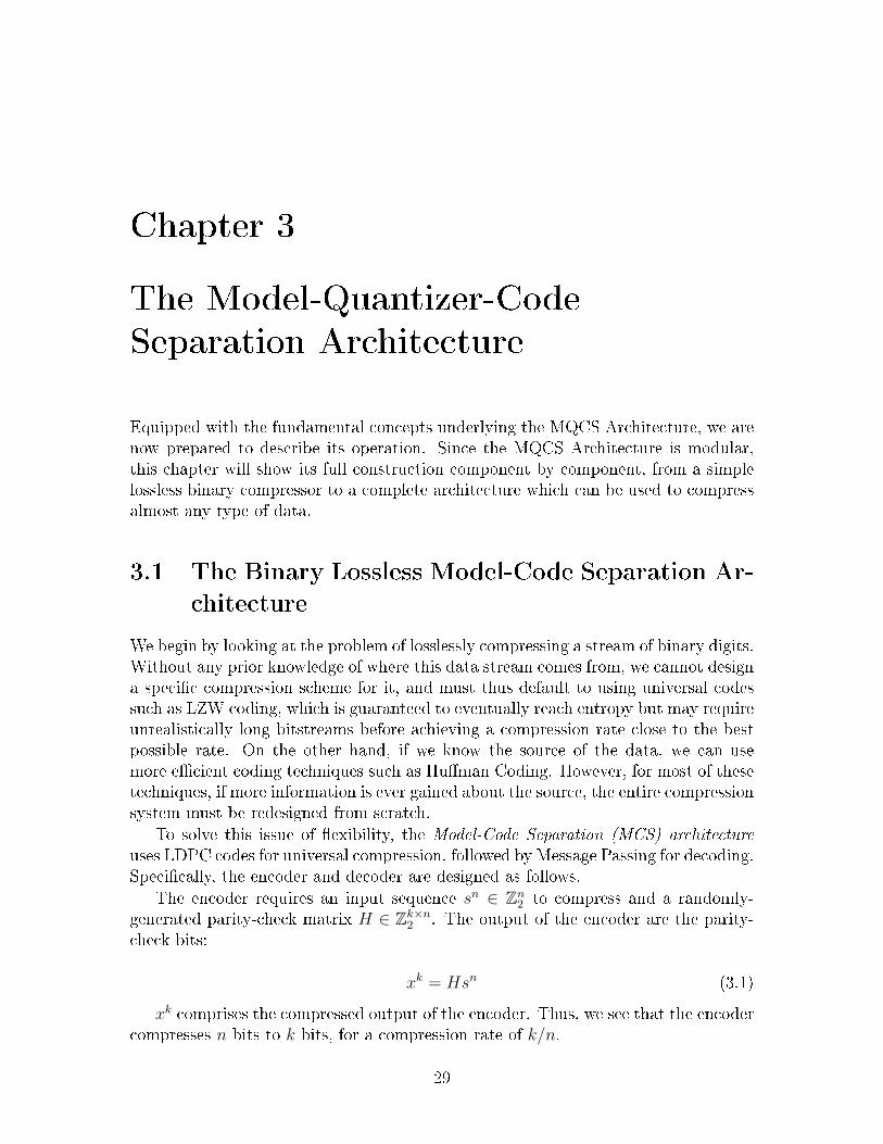
The decoder attempts to reconstruct the original sequence 𝑠𝑛 given the parity-check bits 𝑥𝑘. Since the mapping from 𝑠𝑛 to 𝑥𝑘 is many-to-one for a given 𝐻, thedecoder requires additional information in order to determine the correct reconstruc-tion. This is provided in the form of a source or data model 𝑝𝑠𝑛 , which gives theprobabilities of each source sequence occurring. 𝑝𝑠𝑛 , as a probability distribution, canbe modeled using a PGM of some sort and thus, by combining 𝑥𝑘, 𝐻, and 𝑝𝑠𝑛 , we canconstruct a single graphical model to model the information present in the decoder(see Figure 3-1).

Figure 3-1: The Model-Code-Separation graphical model for binary alphabet sources used

by the decoder, containing both the source and code subgraphs

In particular, we can divide the graph into two distinct subgraphs: the code sub-graph and the source subgraph. The code subgraph is a factor graph which imposesthe parity-check constraints set by 𝐻 and 𝑥𝑘, forcing the source sequence to hash tothe correct parity-check values.

The source subgraph contains the information about the data model given in 𝑝𝑠𝑛 .Depending on the form 𝑝𝑠𝑛 takes, we may use a factor graph, undirected graphi-cal model, or pairwise graphical model to represent the distribution. In each case,this portion of the graph provides information on which configurations of the sourcesequence are more likely to occur, which is important in disambiguating betweenpossible reconstructions.

When both subgraphs are combined, we obtain a distribution whose probabilitiesare nonzero only for certain valid sequences depending on the code graph, and wherethe likelihood of the valid source sequences differ based on the source graph. Ourgoal, then, is to determine the source sequence of highest probability which satisfiesthe parity-check constraints. This can be achieved by running LBP on the graph untilconvergence, then taking the output marginal probabilities 𝑝𝑖(𝑠𝑖), and outputting themaximal probability sequence

𝑠𝑖 = arg max𝑠𝑖

𝑝𝑖(𝑠𝑖), 𝑖 = 1, ..., 𝑛 (3.2)

30

Given that 𝑘/𝑛 exceeds the entropy rate of 𝑝𝑖(𝑠𝑖), and with sufficiently well-designed𝐻, each instance of 𝑥𝑘 should map to only one typical sequence of 𝑠𝑛 [15], andthus the maximal probability sequence 𝑠𝑛 returned will almost certainly be the correctsource sequence, thus achieving perfect reconstruction and thus lossless compressionat rate 𝑘/𝑛.

3.2 Non-Binary Alphabets: the Complete Model-

Code Separation Architecture

While the compressor described in Section 3.1 can achieve universal lossless compres-sion with source-adaptive decoding of binary-alphabet data, it is still unable to handlesequences drawn from larger-alphabet sources. To compensate for this, we introducea translator 𝑇 (𝑠𝑛) into our architecture.

Consider a source sequence 𝑠𝑛 of length 𝑛 where each element is drawn from afinite alphabet 𝒳 of size 𝑝 (WLOG, we can assume that 𝒳 = Z𝑝, so that 𝑠𝑛 ∈ Z𝑛

𝑝 ).Then the translator is an element-wise operator which maps each element 𝑠𝑖 in 𝑠

𝑛 toa sequence of 𝑏 bits 𝑧𝑏𝑖, 𝑧𝑏𝑖+1, ..., 𝑧𝑏𝑖+𝑏−1. For this thesis, we will assume that 𝑝 is apower of 2, and thus can be represented with 𝑏 = log 𝑝 bits. Thus, 𝑇 maps 𝑠𝑛 ∈ Z𝑛

𝑝

to 𝑧𝑛𝑏 ∈ Z𝑛𝑏2 , and

(𝑧𝑏𝑖, 𝑧𝑏𝑖+1, ..., 𝑧𝑏𝑖+𝑏−1) = 𝑡(𝑠𝑖) (3.3)

Where 𝑡(𝑠) is a single instance of the function 𝑇 (𝑠𝑛) applied to a single scalarelement. Examples of 𝑡(𝑠) include binary codes and Gray codes. Because 𝑇 (𝑠𝑛) isan element-wise operator, we can easily model it using a factor graph. Specifically,we can add a series of factor nodes 𝑡1, 𝑡2, ..., 𝑡𝑛, with each factor node imposing thetranslator constraints in a similar fashion to how the factor nodes in the code graphenforce the parity-check constraints. That is, for a factor node 𝑡𝑖 connected to 𝑠𝑖 and{𝑧𝑏𝑖, 𝑧𝑏𝑖+1, ..., 𝑧𝑏𝑖+𝑏−1},

𝑓𝑡𝑖(𝑠𝑖, 𝑧𝑏𝑖, 𝑧𝑏𝑖+1, ..., 𝑧𝑏𝑖+𝑏−1) = 1{𝑡(𝑠𝑖) == {𝑧𝑏𝑖+𝑘}𝑏−1𝑘=0} (3.4)

With the addition of this translator, we can now provide an updated system forthe lossless compression of data drawn from any finite alphabet. The encoder nowtakes in an input sequence 𝑠𝑛 ∈ Z𝑛

𝑝 , passes it through 𝑇 (𝑠𝑛) to produce 𝑧𝑛𝑏 ∈ Z𝑛𝑏2 . 𝑧𝑛𝑏

is then passed through the parity-check matrix 𝐻 ∈ Z𝑘×𝑛𝑏2 to produce the parity-check

bits 𝑥𝑘, which is the compressed output of the encoder.

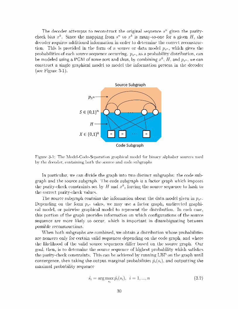
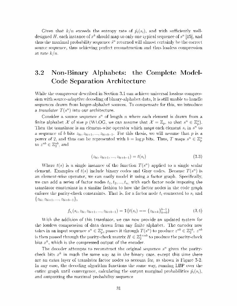
The decoder attempts to reconstruct the original sequence 𝑠𝑛 given the parity-check bits 𝑥𝑘 in much the same way as in the binary case, except this time thereare an extra layer of translator factor nodes to account for, as shown is Figure 3-2.In any case, the decoding algorithm functions the same way, running LBP over theentire graph until convergence, calculating the output marginal probabilities 𝑝𝑖(𝑠𝑖),and outputting the maximal probability sequence

31

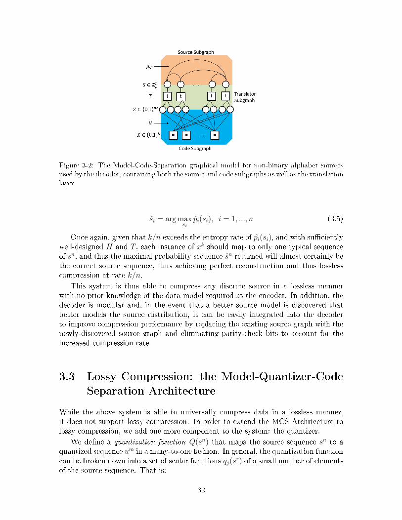
Figure 3-2: The Model-Code-Separation graphical model for non-binary alphabet sources

used by the decoder, containing both the source and code subgraphs as well as the translation

layer

𝑠𝑖 = arg max𝑠𝑖

𝑝𝑖(𝑠𝑖), 𝑖 = 1, ..., 𝑛 (3.5)

Once again, given that 𝑘/𝑛 exceeds the entropy rate of 𝑝𝑖(𝑠𝑖), and with sufficientlywell-designed 𝐻 and 𝑇 , each instance of 𝑥𝑘 should map to only one typical sequenceof 𝑠𝑛, and thus the maximal probability sequence 𝑠𝑛 returned will almost certainly bethe correct source sequence, thus achieving perfect reconstruction and thus losslesscompression at rate 𝑘/𝑛.

This system is thus able to compress any discrete source in a lossless mannerwith no prior knowledge of the data model required at the encoder. In addition, thedecoder is modular and, in the event that a better source model is discovered thatbetter models the source distribution, it can be easily integrated into the decoderto improve compression performance by replacing the existing source graph with thenewly-discovered source graph and eliminating parity-check bits to account for theincreased compression rate.

3.3 Lossy Compression: the Model-Quantizer-Code

Separation Architecture

While the above system is able to universally compress data in a lossless manner,it does not support lossy compression. In order to extend the MCS Architecture tolossy compression, we add one more component to the system: the quantizer.

We define a quantization function 𝑄(𝑠𝑛) that maps the source sequence 𝑠𝑛 to aquantized sequence 𝑢𝑚 in a many-to-one fashion. In general, the quantization functioncan be broken down into a set of scalar functions 𝑞𝑗(𝑠

𝑟) of a small number of elementsof the source sequence. That is:

32

𝑢𝑗 = 𝑞𝑗(𝑠𝑟𝑞𝑗

), 𝑗 = 1, ...,𝑚 (3.6)

Where 𝑠𝑟𝑞𝑗 is a subset of 𝑠𝑛 and 𝑟 ≪ 𝑛. Depending on the choice of 𝑄(𝑠𝑛), we can

see how this quantization function can achieve lossy encoding. And then, by applyingan appropriate translator 𝑇 to 𝑢𝑚 we can produce a binary sequence 𝑧𝑚𝑏, which canthen be used as the input to the parity-check matrix 𝐻 to produce a compressedoutput 𝑥𝑘, we can achieve lossy compression.

In order to decode, we once again model the entire system as a PGM and runmessage passing to determine an estimate 𝑠𝑛 of the source sequence which maps tothe given parity check bits. To model the quanitzer, we add an extra layer of nodes 𝑄between the translator 𝑇 and the source model 𝑝𝑠𝑛 , which consists of a set of factornodes 𝑞1, ...𝑞𝑚 that impose the quantizer constraints of the system

𝑓𝑞𝑖(𝑠𝑟𝑞𝑖, 𝑢𝑖) = 1{𝑞𝑖(𝑠𝑟𝑞𝑖) == 𝑢𝑖} (3.7)

For the case of binary lossy compression, one choice of 𝑄(𝑠𝑛) that has been shownto be effective is the Low Density Hashing Quantizer (LDHQ) [8]. The LDHQ 𝑄(𝑠𝑛)consists of a set of independent functions 𝑞1(𝑠

𝑟1), ..., 𝑞𝑚(𝑠𝑟𝑚), with each 𝑠𝑟𝑖 consisting of

a random subset of 𝑠𝑛 of size 𝑟. The encoding function is a geometric hash

𝑞𝑖(𝑠𝑟𝑖 ) = 1{𝛿(𝑠𝑟𝑖 , 𝑣𝑟𝑖 ) ≤

𝑟

2} (3.8)

Where 𝛿(𝑢, 𝑣) is the Hamming distance between 𝑢 and 𝑣 and 𝑣𝑟𝑖 is a randomlydrawn binary vector of length 𝑟. By setting 𝑚 < 𝑛, we can achieve lossy compressionat a rate 𝑛

𝑘and a distortion determined by 𝑚.

For the case of compressing a real-valued source sequence, we have shown in jointwork with Lai [21] that the uniform quantizer is an effective model-free quantizer. Theuniform quantization function is an element-wise quantizer which, for each elementof the source sequence 𝑠𝑖, outputs a uniformly quantized output

𝑢𝑖 = ⌊𝑠𝑖𝑤⌋ (3.9)

Where ⌊𝑥⌋ is the floor function (the largest integer smaller than 𝑥), and 𝑤 is awidth parameter used to control the rate and distortion of the reconstruction, withlarger 𝑤 corresponding to lower rate and higher distortion [10, Sec 3.2]. This quantizerhas been shown to be effective for compressing iid and markov Gaussian sources [21].An example of the complete decoder graph for the case of the uniform quantizer canbe found in Figure 3-3.

3.4 Benefits of the Separation Architecture

Having described the architecture we are using for compression, we can now list thebenefits provided by this system.

∙ Model-independent encoding : The MQCS Architecture requires only the source

33

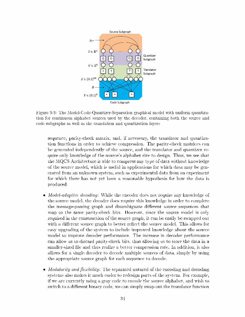
Figure 3-3: The Model-Code-Quantizer-Separation graphical model with uniform quantiza-

tion for continuous alphabet sources used by the decoder, containing both the source and

code subgraphs as well as the translation and quantization layers

sequence, parity-check matrix, and, if necessary, the translator and quantiza-tion functions in order to achieve compression. The parity-check matrices canbe generated independently of the source, and the translator and quantizer re-quire only knowledge of the source’s alphabet size to design. Thus, we see thatthe MQCS Architecture is able to compress any type of data without knowledgeof the source model, which is useful in applications for which data may be gen-erated from an unknown system, such as experimental data from an experimentfor which there has not yet been a reasonable hypothesis for how the data isproduced.

∙ Model-adaptive decoding : While the encoder does not require any knowledge ofthe source model, the decoder does require this knowledge in order to completethe message-passing graph and disambiguate different source sequences thatmap to the same parity-check bits. However, since the source model is onlyrequired in the construction of the source graph, it can be easily be swapped outwith a different source graph to better reflect the source model. This allows foreasy upgrading of the system to include improved knowledge about the sourcemodel to improve decoder performance. The increase in decoder performancecan allow us to discard parity-check bits, thus allowing us to store the data in asmaller-sized file and thus realize a better compression rate. In addition, it alsoallows for a single decoder to decode multiple sources of data, simply by usingthe appropriate source graph for each sequence to decode.

∙ Modularity and flexibility : The separated natured of the encoding and decodingsystems also makes it much easier to redesign parts of the system. For example,if we are currently using a gray code to encode the source alphabet, and wish toswitch to a different binary code, we can simply swap out the translator function

34

in the encoder and decoder without altering any other part of the system. Or,if a better class of codes arise that outperforms LDPC Codes for compression,the code graph can easily be updated to use the new code. Thus, we neverhave to worry about "locking in" any part of the compression system, and wecan quickly alter the encoder or decoder to work with different types of dataor different variations on the system without altering the core algorithms beingimplemented.

∙ Robustness : As discussed by Lai [21], the MQCS Architecture also providesrobustness to errors, since each parity-check bit is independent of the others.By adding more parity-check bits (i.e. decreasing the compression rate), we canallow for some of these bits to be corrupted while still correctly decoding themessage with near certainty.

∙ Speed and efficiency : Compared to other compression methods, the compressionof binary sources in this architecture is very fast, requiring only multiplicationby a sparse matrix, which can be performed in linear time on a CPU or evenfaster on a dedicated chip with support for LDPC Codes. Depending on thechoices of translator and quantizer functions, compressing a source sequencecan be done extremely quickly, and since message-passing is a series of localupdates, it can be computed in a distributed fashion for very rapid decoding aswell.

3.5 Practical Considerations

Now that we have described the theoretical operations of the MQCS Architecture,there are some practical considerations that need to be discussed which will affect theimplementation of this system in code.

3.5.1 Doping

As discussed in [15], often times the decoder cannot converge without some non-trivial initialization of the messages. One method of ensuring a good initialization isdoping, in which a subset of the bits (the doped bits) are transmitted uncompressed,thus initializing the probabilities of these bits to zero or one. This provides a fewpoints to "anchor" the message-passing algorithm and ensure that it converges to thecorrect reconstruction. We define the doping rate 𝑟𝑑𝑜𝑝𝑒 as the fraction of uncompressedbits sent.

𝑟𝑑𝑜𝑝𝑒 =# 𝑜𝑓 𝑑𝑜𝑝𝑒 𝑏𝑖𝑡𝑠 𝑡𝑟𝑎𝑛𝑠𝑚𝑖𝑡𝑡𝑒𝑑

𝑡𝑜𝑡𝑎𝑙 # 𝑜𝑓 𝑢𝑛𝑐𝑜𝑚𝑝𝑟𝑒𝑠𝑠𝑒𝑑 𝑏𝑖𝑡𝑠(3.10)

In general, different models require different doping rates, with more complex mod-els requiring more doped bits. Practically, we can run the encoder and decoder usingdifferent rates to determine empirically what doping rate is optimal for convergence.The actual compression rate 𝑟𝑡𝑜𝑡𝑎𝑙 is thus

35

𝑟𝑡𝑜𝑡𝑎𝑙 = 𝑟𝑑𝑜𝑝𝑒 + 𝑟𝑐𝑜𝑑𝑒 (3.11)

Where 𝑟𝑐𝑜𝑑𝑒 is the code rate, or the fraction of parity-check bits to uncompressedbits.

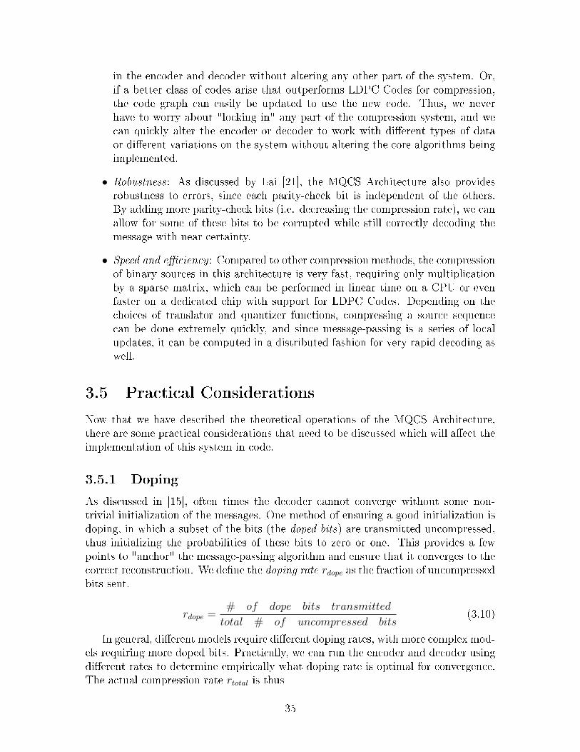
3.5.2 Threshold Rates

When running the encoder/decoder at different rates, we observe three regimes in thedecoder, summarized in Figure 3-4.

Figure 3-4: Plot of decoding errors as a function of compression rate illustrating the three

regimes of operation in a typical application of the MQCS system.

∙ In the first regime, at low rates, LBP does not converge or has a high probabilityof converging to an incorrect reconstruction, due to not having enough parity-check bits to properly disambiguate between different possible reconstructions,and thus compression is not possible at these rate.

∙ In the second regime, at high rates, the system possesses a sufficient number ofparity-check bits and LBP almost certainly converges to the correct reconstruc-tion, thus making compression possible at these rates.

∙ The third regime is a transitional phase between the low-rate regime and thehigh-rate regime, in which some but not all instances of the system can bedecoded correctly, due to variations in source sequences or parity-check matrix

36

patterns at a certain rate. In this regime, compression is sometimes possible, andwith better codes or algorithm implementations, it is possible that compressioncould almost certainly be possible at these rates.

From these observations, we observe two rates of interest:

∙ 𝑟𝑡ℎ𝑟𝑒𝑠ℎ, the threshold rate at which compression first becomes possible (the tran-sitional rate between the first and third regime). Practically, we define it as thepoint at which we observe a 10% success rate in compression.

∙ 𝑟𝑐𝑜𝑛𝑣𝑔, the rate at which compression is almost always possible (the transitionalrate between the third and second regime). Practically, we define it as the pointat which we observe a 90% success rate in compression.

For the purposes of this thesis, we will be using 𝑟𝑡ℎ𝑟𝑒𝑠ℎ as the compression rate, asit reflects the potential ability of the system to compress data at a certain rate [15].

3.6 Summary

In this chapter, we have described the construction and operation of the MQCSArchitecture for the compression of data. We have explained each component of thesystem and how to adapt the system to compress any type of data drawn from anysource alphabet in either a lossy or a lossless fashion. We have also described thebenefits of the system, which motivate our reasons for pursuing the investigation ofthis system. Finally, we touch on a few implementation details which will later berelevant. In the next chapter, we will explore the application of this architecture tothe compression of image data.

37

38

Chapter 4

Image Compression

Now that we have described the MQCS Architecture and summarized its featuresand previous uses, we are now prepared to explore the usage of this architecture inpractical applications. Specifically, we focus on one common use of data compressionsystems: image compression. Natural images tend to have very complex propertieswhich also allow for a high degree of redundancy and thus can be greatly compressed.Furthermore, as discussed in Chapter 1, image compression systems tend to be very"locked-in," with almost no ability to adapt to new developments in image modeling,of which there are many.

4.1 Bi-Level Image Compression

We begin our investigation by looking at image data drawn from a small finite alpha-bet, in this case a binary alphabet where pixels can only take on a value of 0 (black)or 1 (white). Huang [15] has already shown that the 2D homogeneous Ising model issomewhat effective as a source model for compressing binary images. We extend thiswork by investigating an alternative source model which better captures the sourcemodel for images: the Restricted Boltzmann Machine.

4.1.1 RBMs for Bi-Level Image Compression

The RBM is a natural choice of a model to use for images, as previous work hasshown it to be an effective generative model for images, with its ability to capturefeatures of images with its latent nodes [30]. Since the pixels are binary valued, weuse the BRBM as a source model for the images.

4.1.2 Message Passing in BRBMs

In order to use the BRBM in the MQCS Architecture, we must first develop themessage passing equations for the model. Recall that for a BRBM with visible nodes𝑣𝑛, hidden nodes ℎ𝑚, and parameters 𝑏𝑛, 𝑐𝑚,𝑊 𝑛×𝑚, the associated probability distri-bution is

39

𝑝(𝑣𝑛, ℎ𝑚) ∝ 𝑒𝑥𝑝

(𝑛∑

𝑖=1

𝑏𝑖𝑣𝑖 +𝑚∑𝑗=1

𝑐𝑗ℎ𝑗 +

𝑛,𝑚∑𝑖,𝑗

𝑊𝑖𝑗𝑣𝑖ℎ𝑗

)(4.1)

From which we can derive the potential functions

𝜑𝑣𝑖(𝑣𝑖) = 𝑒𝑥𝑝(𝑏𝑖𝑣𝑖), 𝑖 = 1, ..., 𝑛 (4.2)

𝜑ℎ𝑗(ℎ𝑗) = 𝑒𝑥𝑝(𝑐𝑗ℎ𝑗), 𝑗 = 1, ...,𝑚 (4.3)

𝜓𝑣𝑖,ℎ𝑗(𝑣𝑖, ℎ𝑗) = 𝑒𝑥𝑝(𝑊𝑖𝑗𝑣𝑖ℎ𝑗), 𝑖 = 1, ...𝑛, 𝑗 = 1, ...,𝑚 (4.4)

Using these potentials, we can easily evaluate the message passing equation

𝑚(𝑡)𝑣𝑖→ℎ𝑗

(ℎ𝑗) =∑𝑣𝑖

⎛⎝𝜑𝑣𝑖(𝑣𝑖)𝜓𝑣𝑖,ℎ𝑗(𝑣𝑖, ℎ𝑗)

∏ℎ𝑘∈𝑁(𝑣𝑖)∖ℎ𝑗

𝑚(𝑡−1)ℎ𝑘→𝑣𝑖

(𝑣𝑖)

⎞⎠ (4.5)

By inserting the appropriate potential functions, explicitly evaluating the summa-tions, and normalizing the messages, we obtain

𝑚(𝑡)𝑣𝑖→ℎ𝑗

(ℎ𝑗) =1 + 𝑒𝑊𝑖𝑗𝑝𝑣𝑖→ℎ𝑗

2 + (1 + 𝑒𝑊𝑖𝑗)𝑝𝑣𝑖→ℎ𝑗

(4.6)

𝑝𝑣𝑖→ℎ𝑗= 𝑒𝑥𝑝

⎛⎝𝑏𝑖 +∑

𝑘∈𝑁(𝑣𝑖)∖ℎ𝑗

𝑙𝑜𝑔

(𝑚

(𝑡−1)𝑘→𝑖 (1)

𝑚(𝑡−1)𝑘→𝑖 (0)

)⎞⎠ (4.7)

Similarly, the message passing equation from the hidden to the visible nodes is

𝑚(𝑡)ℎ𝑖→𝑣𝑗

(ℎ𝑗) =1 + 𝑒𝑊𝑗𝑖𝑝ℎ𝑖→𝑣𝑗

2 + (1 + 𝑒𝑊𝑗𝑖)𝑝ℎ𝑖→𝑣𝑗

(4.8)

𝑝ℎ𝑖→𝑣𝑗 = 𝑒𝑥𝑝

⎛⎝𝑐𝑖 +∑

𝑘∈𝑁(ℎ𝑖)∖𝑣𝑗

𝑙𝑜𝑔

(𝑚

(𝑡−1)𝑘→𝑖 (1)

𝑚(𝑡−1)𝑘→𝑖 (0)

)⎞⎠ (4.9)

However, while these are the exact message-passing equations, in practice, theydo not perform well in our compression system due to numerical issues, as many ofthe messages tend to take on values very close to 0 or 1, making it difficult to retainprecision even in the log domain as the number of edges grows large.

As such, we use an approximate energy-based method which is much more robustto precision errors. Looking at the energy function for the BRBM, we observe thatby conditioning on the visible layer

𝐸(ℎ𝑗|𝑣𝑛) = −𝑐𝑗ℎ𝑗 −𝑛∑

𝑖=1

𝑊𝑖𝑗𝑣𝑖ℎ𝑗 (4.10)

If we know the independent marginal probabilities of each visible node 𝑝𝑣1(𝑣1),𝑝𝑣2(𝑣2), ..., 𝑝𝑣𝑛(𝑣𝑛), then by taking a weighted average we can obtain the estimate of

40

the energy of ℎ𝑗

𝐸ℎ𝑗(ℎ𝑗) ≈

∑𝑣𝑛

𝐸(ℎ𝑗|𝑣𝑛)𝑛∏

𝑖=1

𝑝𝑣𝑖(𝑣𝑖) = −𝑐𝑗ℎ𝑗 −𝑛∑

𝑖=1

𝑊𝑖𝑗𝑝𝑣𝑖(1)ℎ𝑗 (4.11)

Then, we can compute the marginal probability 𝑝ℎ𝑗(ℎ𝑗) by noting that an approx-

imation of the probability of a node is given by

𝑝(ℎ𝑗) ∝ 𝑒𝑥𝑝(−𝐸ℎ𝑗(ℎ𝑗)) (4.12)

And then normalizing to obtain

𝑝ℎ𝑗(ℎ𝑗 = 1) ≈ 1

1 + 𝑒𝑥𝑝(−𝐸ℎ𝑗(1))

=1

1 + 𝑒𝑥𝑝(−𝑐𝑗 −∑𝑛

𝑖=1𝑊𝑖𝑗𝑝𝑣𝑖(1))(4.13)

Similarly, for the visible nodes

𝑝𝑣𝑖(𝑣𝑖 = 1) ≈ 1

1 + 𝑒𝑥𝑝(−𝐸𝑣𝑖(1))=

1

1 + 𝑒𝑥𝑝(−𝑏𝑖 −∑𝑚

𝑗=1𝑊𝑖𝑗𝑝ℎ𝑗(1))

(4.14)

Thus, we have the following approximate message passing algorithm for the BRBMsource subgraph given in Algorithm 3.

This algorithm is much more robust and has shown to work much more effectivelyin empirical tests performed on the MNIST Database (described in the next section).

4.1.3 Compression of the MNIST Database

We demonstrate the effectiveness of the BRBM as a source model for compression byusing it to compress data drawn from the MNIST Database, a database of imagesof handwritten digits of size 28x28 [23]. As a database of images which have clearpatterns and shared features but still have a very large set of possible realizations, itis a natural choice for compression using the BRBM.

Experimental Setup

Since the MNIST Database is a greyscale image database, we begin by thresholdingthe values at the midpoint between black and white to create a binary image database.We then train a model on a subset of the dataset using the Contrastive Divergencemethod outlined in [12] in order to obtain the model parameters. Once we have ourmodel, we test its effectiveness in the MQCS Architecture by constructing the encoderand decoder for our data source.

The encoder takes in the binary data and applies a randomly-generated LDPCcode of some specified size to generate a sequence of parity-check bits which serve asthe compressed output of the encoder. We also output a small percentage of the bitsuncompressed as doped bits.

n.b. We used code provided in [25] for generating LDPC codes which removes4-cycles in the code graph. Our previous work [21] has shown that 4-cycles interfere

41

Algorithm 3: Message Passing Updates for BRBM

Input: Parameters Θ = (𝑏𝑛, 𝑐𝑚,𝑊 𝑛×𝑚), aggregate messages into subgraph

from rest of graph 𝑚(𝑡−1)𝐺′→𝑣1

,𝑚(𝑡−1)𝐺′→𝑣2

, ...,𝑚(𝑡−1)𝐺′→𝑣𝑛

, normalized marginal

probabilities from previous iterations 𝑝(𝑡−1)ℎ1

(ℎ1), 𝑝(𝑡−1)ℎ2

(ℎ2), ..., 𝑝(𝑡−1)ℎ𝑚

(ℎ𝑚)

Output: Marginal probabilities 𝑝(𝑡)ℎ𝑗

(ℎ𝑗) for all hidden nodes ℎ𝑖 in ℎ𝑛, output

messages from visible nodes to rest of graph𝑚

(𝑡)𝑣1→𝐺′ ,𝑚

(𝑡)𝑣2→𝐺′ , ...,𝑚

(𝑡)𝑣𝑛→𝐺′

//Update visible node probabilitiesfor 𝑖 = 1, ..., 𝑛 do

𝑝𝑣𝑖(1)← 1

1+𝑒𝑥𝑝(−𝑏𝑖−∑𝑚

𝑗=1 𝑊𝑖𝑗𝑝(𝑡−1)ℎ𝑗

(1))

𝑝𝑣𝑖(1)←𝑝𝑣𝑖 (1)𝑚

(𝑡−1)

𝑣𝑖→𝐺′ (1)

𝑝𝑣𝑖 (1)𝑚(𝑡−1)

𝑣𝑖→𝐺′ (1)+(1−𝑝𝑣𝑖 (1))(1−𝑚(𝑡−1)

𝑣𝑖→𝐺′ (1))

end//Update hidden node probabilitiesfor 𝑗 = 1, ...,𝑚 do

𝑝(𝑡)ℎ𝑗

(1)← 11+𝑒𝑥𝑝(−𝑐𝑗−

∑𝑛𝑖=1 𝑊𝑖𝑗𝑝𝑣𝑖 (1))

end//Update visible node probabilities again and set them as output messagesfor 𝑖 = 1, ..., 𝑛 do

𝑚(𝑡)𝑣𝑖→𝐺′(1)← 1

1+𝑒𝑥𝑝(−𝑏𝑖−∑𝑚

𝑗=1 𝑊𝑖𝑗𝑝(𝑡)ℎ𝑗

(1))

end

return 𝑝(𝑡)ℎ𝑗

(ℎ1), 𝑗 = 1, ...,𝑚 and 𝑚(𝑡)𝑣𝑖→𝐺′(𝑣𝑖), 𝑖 = 1, ..., 𝑛

with message-passing performance and reduce the effectiveness of compression.The decoder takes in the parity-check and doped bits, the parity-check matrix,

and the BRBM model parameters and uses them to construct a graphical model ofthe data as in Figure 4-1. We then run loopy belief propagation to decode the originaldata, using the doped bits to initialize our messages. We run the algorithm for onehundred iterations or until it converges (that is, the marginal probability of any onebit does not change by more than a small threshold value between iterations) andthreshold the output probability at 0.5 to obtain an estimated binary reconstructionof the data. In order to determine the compression rate, we run the encoder anddecoder for multiple parity-check matrices at a variety of different coding rates anddoping rates, with 10 different parity-check matrices tested for each image at eachrate. We then extract the threshold and convergent compression rates by looking forthe total rates at which the source sequence can first be successfully decoded 1/10and 10/10 times, respectively.

We compare these values with the same system but with the source model inthe decoder replaced with the non-homogeneous Ising Model (where each edge has adifferent potential instead of sharing a single potential parameter), which has beenshown to outperform the general compression algorithm GZIP. We estimate the Ising

42

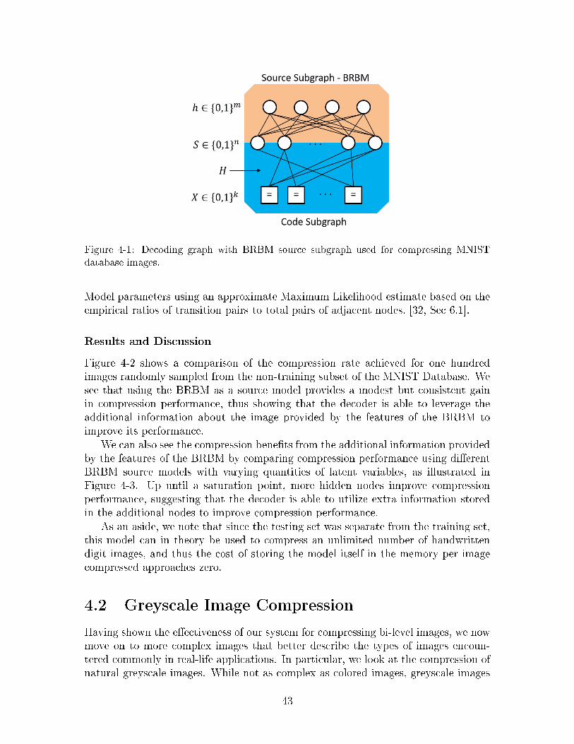
Figure 4-1: Decoding graph with BRBM source subgraph used for compressing MNIST

database images.

Model parameters using an approximate Maximum Likelihood estimate based on theempirical ratios of transition pairs to total pairs of adjacent nodes. [32, Sec 6.1].

Results and Discussion

Figure 4-2 shows a comparison of the compression rate achieved for one hundredimages randomly sampled from the non-training subset of the MNIST Database. Wesee that using the BRBM as a source model provides a modest but consistent gainin compression performance, thus showing that the decoder is able to leverage theadditional information about the image provided by the features of the BRBM toimprove its performance.

We can also see the compression benefits from the additional information providedby the features of the BRBM by comparing compression performance using differentBRBM source models with varying quantities of latent variables, as illustrated inFigure 4-3. Up until a saturation point, more hidden nodes improve compressionperformance, suggesting that the decoder is able to utilize extra information storedin the additional nodes to improve compression performance.

As an aside, we note that since the testing set was separate from the training set,this model can in theory be used to compress an unlimited number of handwrittendigit images, and thus the cost of storing the model itself in the memory per imagecompressed approaches zero.

4.2 Greyscale Image Compression

Having shown the effectiveness of our system for compressing bi-level images, we nowmove on to more complex images that better describe the types of images encoun-tered commonly in real-life applications. In particular, we look at the compression ofnatural greyscale images. While not as complex as colored images, greyscale images

43

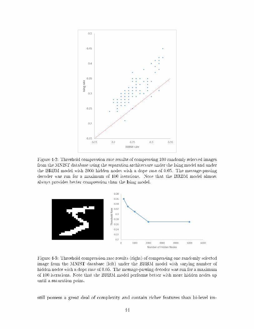
Figure 4-2: Threshold compression rate results of compressing 100 randomly selected images

from the MNIST database using the separation architecture under the Ising model and under

the BRBM model with 2000 hidden nodes with a dope rate of 0.05. The message-passing

decoder was run for a maximum of 100 iterations. Note that the BRBM model almost

always provides better compression than the Ising model.

Figure 4-3: Threshold compression rate results (right) of compressing one randomly selected

image from the MNIST database (left) under the BRBM model with varying number of

hidden nodes with a dope rate of 0.05. The message-passing decoder was run for a maximum

of 100 iterations. Note that the BRBM model performs better with more hidden nodes up

until a saturation point.

still possess a great deal of complexity and contain richer features than bi-level im-

44

ages. They also allow us to explore the regime of lossy compression, as full-resolutiongreyscale images tend to require a large amount of memory to store losslessly.

4.2.1 RBMs for Greyscale Image Compression

Once again, in order to capture the complex features of natural greyscale images, welook to the RBM, this time utilizing the GRBM as a source model. While in theoryit would be possible to use a BRBM to model the relationships between all the bitsused in encoding all the pixels, a GRBM is a far better model to use due to the nearlycontinuous nature of the pixel distributions and the fact that GRBMs have a muchlower complexity compared to modeling each individual bit of the image rather thanthe pixels.

4.2.2 Message Passing in GRBMs

As with the BRBM, we must first develop the message passing updates for the GRBMbefore we can use it in our compression scheme. However, unlike the BRBM, theexact message update expressions quickly becomes intractable due to an exponentialscaling in time complexity with respect to the number of hidden nodes in messagecomputation.

To see where this scaling arises, we begin by computing the messages from the hid-den nodes to the visible nodes. Recall that for a GRBM with visible nodes 𝑣𝑛, hiddennodes ℎ𝑚, and parameters 𝑏𝑛, 𝑐𝑚, 𝜎𝑛,𝑊 𝑛×𝑚, the associated probability distribution is

𝑝(𝑣𝑛, ℎ𝑚) ∝ 𝑒𝑥𝑝

(−1

2

𝑛∑𝑖=1

(𝑣𝑖 − 𝑏𝑖)2

𝜎2𝑖

+𝑚∑𝑗=1

𝑐𝑗ℎ𝑗 +

𝑛,𝑚∑𝑖,𝑗

𝑊𝑖𝑗𝑣𝑖ℎ𝑗

)(4.15)

Which gives the following potentials

𝜑𝑣𝑖(𝑣𝑖) = 𝑒𝑥𝑝

(−1

2

(𝑣𝑖 − 𝑏𝑖)2

𝜎2𝑖

), 𝑖 = 1, ..., 𝑛 (4.16)

𝜑ℎ𝑗(ℎ𝑗) = 𝑒𝑥𝑝(𝑐𝑗ℎ𝑗), 𝑗 = 1, ...,𝑚 (4.17)

𝜓𝑣𝑖,ℎ𝑗(𝑣𝑖, ℎ𝑗) = 𝑒𝑥𝑝(𝑊𝑖𝑗𝑣𝑖ℎ𝑗), 𝑖 = 1, ...𝑛, 𝑗 = 1, ...,𝑚 (4.18)

The associated message passing equation for hidden nodes to visible nodes is:

𝑚(𝑡)ℎ𝑗→𝑣𝑖

(𝑣𝑖) =∑ℎ𝑗

⎛⎝𝜑ℎ𝑗(ℎ𝑗)𝜓𝑣𝑖,ℎ𝑗

(𝑣𝑖, ℎ𝑗)∏

𝑣𝑘∈𝑁(ℎ𝑗)∖𝑣𝑖

𝑚(𝑡−1)𝑣𝑘→ℎ𝑗

(ℎ𝑗)

⎞⎠ (4.19)

By inserting the appropriate potential functions, explicitly evaluating the summa-tions, and rescaling the messages, we obtain

𝑚(𝑡)ℎ𝑗→𝑣𝑖

(𝑣𝑖) = 𝑝ℎ𝑗→𝑣𝑖(0) + 𝑝ℎ𝑗→𝑣𝑖(1)𝑒𝑥𝑝(𝑊𝑖,𝑗𝑣𝑖) (4.20)

Where

45

𝑝ℎ𝑗→𝑣𝑖(𝑥) =∏

𝑣𝑘∈𝑁(ℎ𝑗)∖𝑣𝑖

𝑚(𝑡−1)𝑣𝑘→ℎ𝑗

(𝑥), 𝑥 ∈ {0, 1} (4.21)

Using these messages, we can now attempt to compute the message updates fromthe visible to the hidden nodes.

𝑚(𝑡)𝑣𝑖→ℎ𝑗

(ℎ𝑗) =

∫𝑣𝑖

⎛⎝𝜑𝑣𝑖(𝑣𝑖)𝜓𝑣𝑖,ℎ𝑗(𝑣𝑖, ℎ𝑗)

∏ℎ𝑘∈𝑁(𝑣𝑖)∖ℎ𝑗

𝑚(𝑡−1)ℎ𝑘→𝑣𝑖

(𝑣𝑖)

⎞⎠=

∫𝑣𝑖

⎛⎝𝑒𝑥𝑝(−1

2

(𝑣𝑖 − 𝑏𝑖)2

𝜎2𝑖

+𝑊𝑖𝑗𝑣𝑖ℎ𝑗

) ∏ℎ𝑘∈𝑁(𝑣𝑖)∖ℎ𝑗

(𝑝ℎ𝑘→𝑣𝑖(0) + 𝑝ℎ𝑗→𝑣𝑖(1)𝑒𝑥𝑝(𝑊𝑖,𝑗𝑣𝑖))

⎞⎠(4.22)

Expanding this expression out yields an exponential number of squared exponen-tial terms, making the message computation intractable. Thus, we instead derivea close approximation of the message passing updates by looking at estimates ofmarginal probabilities of nodes

We begin by approximating the visible node distributions as Gaussian distribu-tions, an approximations which holds very well when there is a high degree of certaintyas to which features are on or off. For the hidden nodes, we note that the probabilityof a single node is

𝑝ℎ𝑗(ℎ𝑗) ∝

∫𝑣𝑛𝑒𝑥𝑝(−𝐸(ℎ𝑗, 𝑣

𝑛)) =

∫𝑣𝑛𝑒𝑥𝑝

(𝑐𝑗ℎ𝑗 +

𝑛∑𝑖=1

(−1

2

(𝑣𝑖 − 𝜇𝑣𝑖)2

𝜎2𝑣𝑖

+𝑊𝑖𝑗ℎ𝑗𝑣𝑖

))(4.23)

Where 𝜇𝑣𝑖 , 𝜎2𝑣𝑖are the marginal mean and variance of the visible node 𝑣𝑖. Evalu-

ating this integral for ℎ𝑗 = 0 and ℎ𝑗 = 1 and then normalizing the terms yields

𝑝ℎ𝑗(ℎ𝑗 = 1) =

1

1 + 𝑒𝑥𝑝(−𝑏𝑖 −

∑𝑛𝑖=1

(𝑊𝑖𝑗𝜇𝑣𝑖 +𝑊 2

𝑖𝑗𝜎2𝑣𝑖

)) (4.24)

For the visible nodes, we can use an analogous energy argument as in the BRBMcase. The average energy of a visible node is given by

𝐸𝑣𝑖(𝑣𝑖) ∝∑ℎ𝑚

𝐸(𝑣𝑖|ℎ𝑚)𝑚∏𝑗=1

𝑝ℎ𝑗(ℎ𝑗) =

1

2

(𝑣𝑖 − 𝑏𝑖)2

𝜎2𝑖

−𝑚∑𝑗=1

𝑊𝑖𝑗𝑝ℎ𝑗(1)𝑣𝑖 (4.25)

As in the BRBM, we approximate the distribution of 𝑣𝑖 by

𝑝(𝑣𝑖) ∝ 𝑒𝑥𝑝(−𝐸ℎ𝑗(ℎ𝑗)) (4.26)

By completing the square on the energy function and then extracting the scale

46

Algorithm 4: Message Passing Updates for GRBM

Input: Parameters Θ = (𝑏𝑛, 𝑐𝑚, 𝜎𝑛,𝑊 𝑛×𝑚), aggregate means and variances ofthe Gaussian messages into subgraph from rest of graph𝜇(𝑡−1)𝐺′→𝑣1

, 𝜇(𝑡−1)𝐺′→𝑣2

, ..., 𝜇(𝑡−1)𝐺′→𝑣𝑛

, 𝜎2(𝑡−1)𝐺′→𝑣1

, 𝜎2(𝑡−1)𝐺′→𝑣2

, ..., 𝜎2(𝑡−1)𝐺′→𝑣𝑛

,, normalizedmarginal probabilities from previous iterations𝑝(𝑡−1)ℎ1

(ℎ1), 𝑝(𝑡−1)ℎ2

(ℎ2), ..., 𝑝(𝑡−1)ℎ𝑚

(ℎ𝑚)

Output: Marginal probabilities 𝑝(𝑡)ℎ𝑗

(ℎ𝑗) for all hidden nodes ℎ𝑖 in ℎ𝑛, output

means and variances of the Gaussian messages from visible nodes torest of graph 𝜇

(𝑡)𝑣1→𝐺′ , 𝜇

(𝑡)𝑣2→𝐺′ , ..., 𝜇

(𝑡)𝑣𝑛→𝐺′ , 𝜎

2(𝑡)𝑣1→𝐺′ , 𝜎

2(𝑡)𝑣2→𝐺′ , ..., 𝜎

2(𝑡)𝑣𝑛→𝐺′

//Update visible node probabilitiesfor 𝑖 = 1, ..., 𝑛 do

𝜎2𝑣𝑖← 1

1

𝜎2𝑣𝑖→𝐺′

+ 1

𝜎2𝑖

𝜇𝑣𝑖 ←(

𝜇𝑣𝑖→𝐺′

𝜎2𝑣𝑖→𝐺′

+ 𝑏𝑖𝜎2𝑖

)𝜎2𝑣𝑖

𝜇𝑣𝑖 ← 𝜇𝑣𝑖 + 𝜎2𝑣𝑖

∑𝑚𝑗=1𝑊𝑖𝑗𝑝

(𝑡−1)ℎ𝑗

(1)

end//Update hidden node probabilitiesfor 𝑗 = 1, ...,𝑚 do

𝑝(𝑡)ℎ𝑗

(1)← 1

1+𝑒𝑥𝑝(−𝑐𝑗−∑𝑛

𝑖=1(𝑊𝑖𝑗𝜇𝑣𝑖+𝑊 2𝑖𝑗𝜎

2𝑣𝑖))

end//Update visible node probabilities again and set them as output messagesfor 𝑖 = 1, ..., 𝑛 do

𝜇(𝑡)𝑣𝑖→𝐺′ ← 𝑏𝑖 + 𝜎2

𝑖

∑𝑚𝑗=1𝑊𝑖𝑗𝑝

(𝑡−1)ℎ𝑗

(1)

𝜎2(𝑡)𝑣𝑖→𝐺′ ← 𝜎2

𝑣𝑖

end

return 𝑝(𝑡)ℎ𝑗

(ℎ1), 𝑗 = 1, ...,𝑚 and 𝜇(𝑡)𝑣𝑖→𝐺′ , 𝜎

2(𝑡)𝑣𝑖→𝐺′ , 𝑖 = 1, ..., 𝑛

factor, we obtain𝑝(𝑣𝑖) ∼ 𝑁(𝑣𝑖;𝜇𝑣𝑖 , 𝜎

2𝑖 ) (4.27)

𝜇𝑣𝑖 = 𝑏𝑖 + 𝜎2𝑖

𝑚∑𝑗=1

𝑊𝑖𝑗𝑝ℎ𝑗(1) (4.28)

Thus, we obtain the message passing algorithm for a GRBM given in Algorithm4.

4.2.3 Compression of the Cifar-10 Database

We demonstrate the effectiveness of the GRBM as a source model for compression byusing it to compress data drawn from the Cifar-10 Database, a database of labelednatural greyscale images of size 32x32 [19].

47

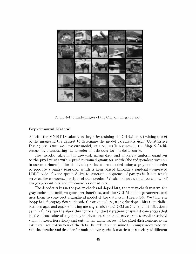
Figure 4-4: Sample images of the Cifar-10 image dataset.

Experimental Method

As with the MNIST Database, we begin by training the GRBM on a training subsetof the images in the dataset to determine the model parameters using ConstrastiveDivergence. Once we have our model, we test its effectiveness in the MQCS Archi-tecture by constructing the encoder and decoder for our data source.

The encoder takes in the greyscale image data and applies a uniform quantizerto the pixel values with a pre-determined quantizer width (the independent variablein our experiment). The bin labels produced are encoded using a gray code in orderto produce a binary sequence, which is then passed through a randomly-generatedLDPC code of some specified size to generate a sequence of parity-check bits whichserve as the compressed output of the encoder. We also output a small percentage ofthe gray-coded bits uncompressed as doped bits.

The decoder takes in the parity-check and doped bits, the parity-check matrix, thegray coder and uniform quantizer functions, and the GRBM model parameters anduses them to construct a graphical model of the data as in Figure 4-5. We then runloopy belief propagation to decode the original data, using the doped bits to initializeour messages and approximating messages into the GRBM as Gaussian distributions,as in [21]. We run the algorithm for one hundred iterations or until it converges (thatis, the mean value of any one pixel does not change by more than a small thresholdvalue between iterations) and output the mean values of the pixel distributions as anestimated reconstruction of the data. In order to determine the compression rate, werun the encoder and decoder for multiple parity-check matrices at a variety of different

48

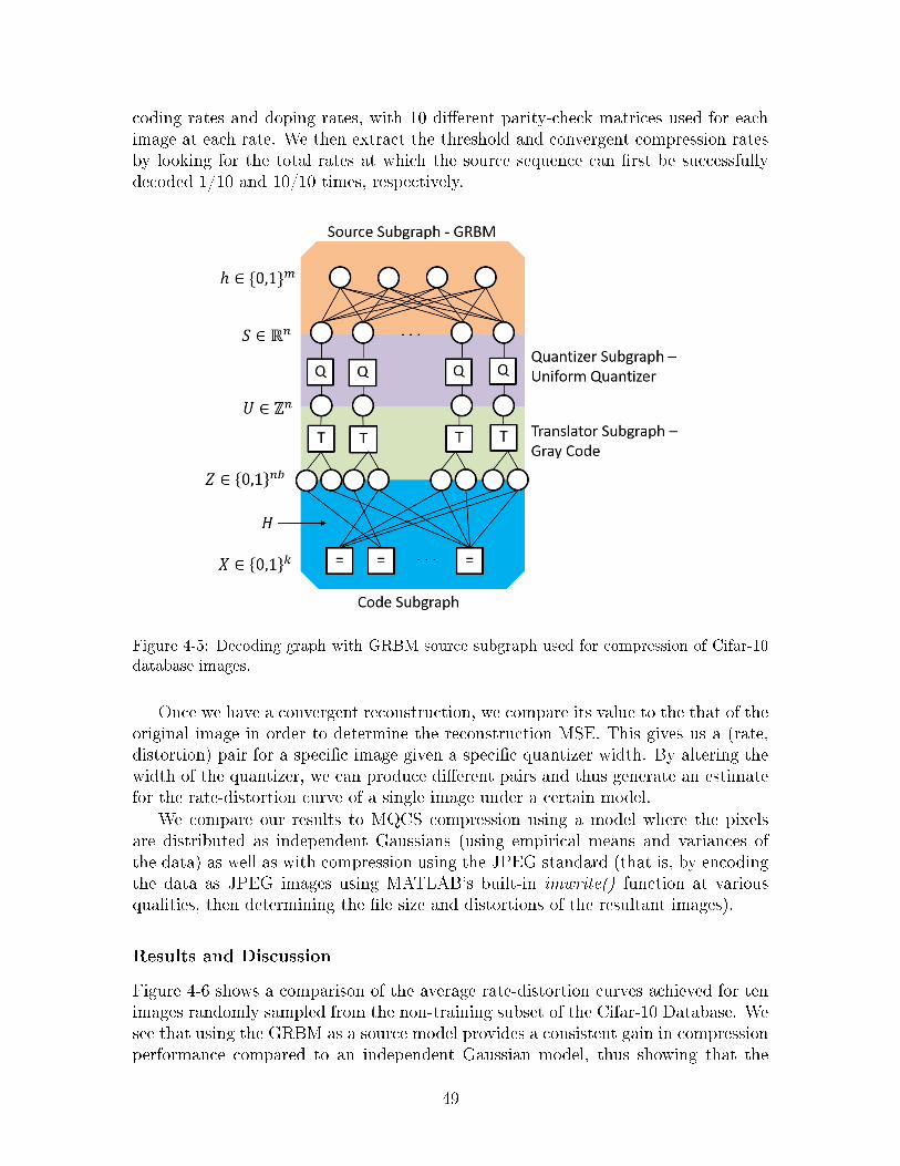
coding rates and doping rates, with 10 different parity-check matrices used for eachimage at each rate. We then extract the threshold and convergent compression ratesby looking for the total rates at which the source sequence can first be successfullydecoded 1/10 and 10/10 times, respectively.

Figure 4-5: Decoding graph with GRBM source subgraph used for compression of Cifar-10

database images.

Once we have a convergent reconstruction, we compare its value to the that of theoriginal image in order to determine the reconstruction MSE. This gives us a (rate,distortion) pair for a specific image given a specific quantizer width. By altering thewidth of the quantizer, we can produce different pairs and thus generate an estimatefor the rate-distortion curve of a single image under a certain model.

We compare our results to MQCS compression using a model where the pixelsare distributed as independent Gaussians (using empirical means and variances ofthe data) as well as with compression using the JPEG standard (that is, by encodingthe data as JPEG images using MATLAB’s built-in imwrite() function at variousqualities, then determining the file size and distortions of the resultant images).

Results and Discussion

Figure 4-6 shows a comparison of the average rate-distortion curves achieved for tenimages randomly sampled from the non-training subset of the Cifar-10 Database. Wesee that using the GRBM as a source model provides a consistent gain in compressionperformance compared to an independent Gaussian model, thus showing that the

49

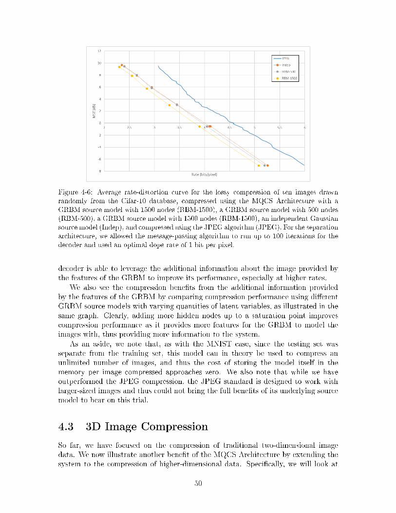
Figure 4-6: Average rate-distortion curve for the lossy compression of ten images drawn

randomly from the Cifar-10 database, compressed using the MQCS Architecture with a

GRBM source model with 1500 nodes (RBM-1500), a GRBM source model with 500 nodes

(RBM-500), a GRBM source model with 1500 nodes (RBM-1500), an independent Gaussian

source model (Indep), and compressed using the JPEG algorithm (JPEG). For the separation

architecture, we allowed the message-passing algorithm to run up to 100 iterations for the

decoder and used an optimal dope rate of 1 bit per pixel.

decoder is able to leverage the additional information about the image provided bythe features of the GRBM to improve its performance, especially at higher rates.

We also see the compression benefits from the additional information providedby the features of the GRBM by comparing compression performance using differentGRBM source models with varying quantities of latent variables, as illustrated in thesame graph. Clearly, adding more hidden nodes up to a saturation point improvescompression performance as it provides more features for the GRBM to model theimages with, thus providing more information to the system.

As an aside, we note that, as with the MNIST case, since the testing set wasseparate from the training set, this model can in theory be used to compress anunlimited number of images, and thus the cost of storing the model itself in thememory per image compressed approaches zero. We also note that while we haveoutperformed the JPEG compression, the JPEG standard is designed to work withlarger-sized images and thus could not bring the full benefits of its underlying sourcemodel to bear on this trial.

4.3 3D Image Compression

So far, we have focused on the compression of traditional two-dimensional imagedata. We now illustrate another benefit of the MQCS Architecture by extending thesystem to the compression of higher-dimensional data. Specifically, we will look at

50

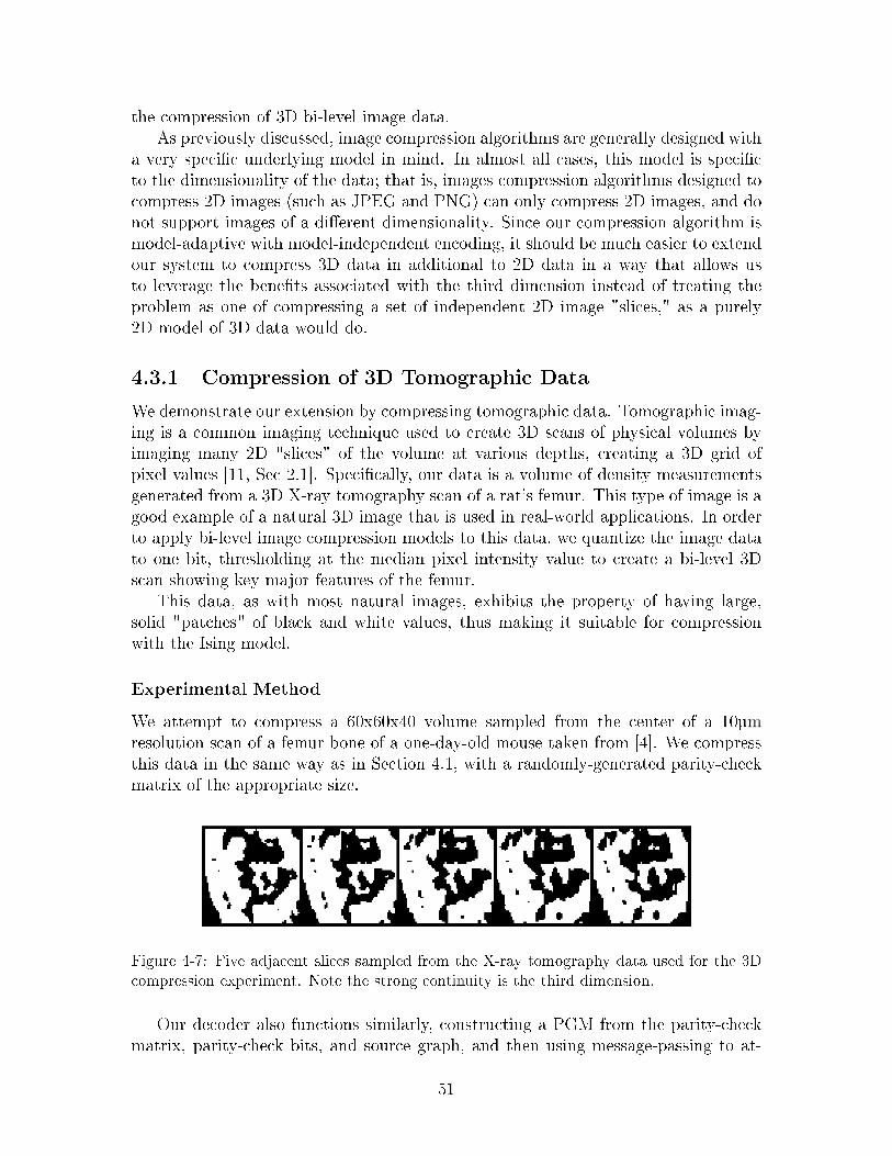
the compression of 3D bi-level image data.As previously discussed, image compression algorithms are generally designed with

a very specific underlying model in mind. In almost all cases, this model is specificto the dimensionality of the data; that is, images compression algorithms designed tocompress 2D images (such as JPEG and PNG) can only compress 2D images, and donot support images of a different dimensionality. Since our compression algorithm ismodel-adaptive with model-independent encoding, it should be much easier to extendour system to compress 3D data in additional to 2D data in a way that allows usto leverage the benefits associated with the third dimension instead of treating theproblem as one of compressing a set of independent 2D image "slices," as a purely2D model of 3D data would do.

4.3.1 Compression of 3D Tomographic Data

We demonstrate our extension by compressing tomographic data. Tomographic imag-ing is a common imaging technique used to create 3D scans of physical volumes byimaging many 2D "slices" of the volume at various depths, creating a 3D grid ofpixel values [11, Sec 2.1]. Specifically, our data is a volume of density measurementsgenerated from a 3D X-ray tomography scan of a rat’s femur. This type of image is agood example of a natural 3D image that is used in real-world applications. In orderto apply bi-level image compression models to this data, we quantize the image datato one bit, thresholding at the median pixel intensity value to create a bi-level 3Dscan showing key major features of the femur.

This data, as with most natural images, exhibits the property of having large,solid "patches" of black and white values, thus making it suitable for compressionwith the Ising model.

Experimental Method

We attempt to compress a 60x60x40 volume sampled from the center of a 10µmresolution scan of a femur bone of a one-day-old mouse taken from [4]. We compressthis data in the same way as in Section 4.1, with a randomly-generated parity-checkmatrix of the appropriate size.

Figure 4-7: Five adjacent slices sampled from the X-ray tomography data used for the 3D

compression experiment. Note the strong continuity is the third dimension.

Our decoder also functions similarly, constructing a PGM from the parity-checkmatrix, parity-check bits, and source graph, and then using message-passing to at-

51

tempt to reconstruct the original image. To illustrate the added benefits of includinga third dimension of correlation, we compare two different source models: a 3D ho-mogeneous Ising Model and a series of 2D homogeneous Ising Models.

For the 3D Ising Model, we assume a homogeneous model similar to the 2Dcase described in Section 2.4.2, except over a 3D lattice (see Figure 4-8 (left)). Thepotentials remain the same; that is:

𝜑𝑖(𝑣𝑖) = [1− 𝑝; 𝑝](𝑣𝑖) (4.29)

𝜓𝑖,𝑗(𝑣𝑖, 𝑣𝑗) =

[𝑞 1− 𝑞

1− 𝑞 𝑞

](𝑣𝑖, 𝑣𝑗), ∀(𝑖, 𝑗) ∈ 𝐸 (4.30)

Where we use ML methods once again to determine the parameters 𝑝 and 𝑞 [32, Sec6.1]. Since the same "patchy" property extends in the third dimension, we believethis extension of the Ising model would also be effective for 3D images of this type.

Our comparison model is a series of independent homogeneous 2D Ising Models,with the width and depth dimensions correlated but the height dimension indepen-dent (see Figure 4-8 (right)). For fairness, we assume that all layers share the sameparameters, so that both the 2D and 3D models have the same amount of param-eter information available to describe the models. We attempt compression of thisvolume using both these sources, as well as using the GZIP algorithm (using MAT-LAB’s built-in gzip() function on a zig-zag scan of the pixels), a universal compressionalgorithm.

Figure 4-8: A 3×3×3 three-dimensional lattice graph (left) and three 3×3 two-dimensional

lattice graphs stacked on top of each other (right), which are examples of the two structures

of the pairwise graphical models representing their respective Ising distributions. Note that

in the stacked 2D case, each layer is independent of all other layers.

Results and Discussion

As seen in Table 4.1, the 3D Ising Model produces the best compression, beating outboth the 2D Ising Model and the GZIP algorithm. Thus, we have shown for this

52

Compression Type Compression Rate

MQCS with 3D Ising Model 0.305MQCS with 2D Ising Model 0.339GZIP 0.582

Table 4.1: Compression results for 60x60x40 3D tomography image. For the MQCS Ar-

chitecture, threshold rates were used with a 0.125 doping rate and a maximum of 300

message-passing iterations.

example that the extra information provided by the extra correlation in the thirddimension can be leveraged by our architecture to improve compression performance.

However, despite the heavy degree of correlation between pixels in the third di-mension (𝑞 ≈ 0.92), the compression gain between the two Ising Models is quitesmall. The primary reason for this is likely the limitations of the LDPC code whenused as a data compressor. Lai [21] has noted that the optimal node degree for eachparity-check bit is 3, but at low rates (specifically, rates below 1

3), it is impossible

to construct a code that has an average factor degree of 3 and where each bit to becompressed is connected to at least one parity-check factor node. Thus, as the com-pression decreases, the average node degree must by necessity increase, thus makingthe LDPC code less effective [26]. From this data, we believe that the code ratesoft limit where the LDPC code begins to severely under-perform for compression isaround 0.17 to 0.18.

4.4 Summary and Remarks

In this chapter, we have explored three different realizations of the MQCS Architec-ture for three different applications. In the first two, we have shown that RestrictedBoltzmann Machines are effective source models for compression due to their abil-ity to store information about image features in its latent variables. In the third,we showed how our architecture was able to easily leverage additional dimensionalinformation in order to improve compression performance.

In these three applications, we have illustrated the flexibility and adaptability ofthis compression architecture. We were able to modify the architecture to compresseach data source using only minor modifications or additions to the encoder and de-coder, none of which altered the fundamental algorithms used in the system (hashingfor encoding and message-passing for decoding). Within each application, we wereable to rapidly "upgrade" the system by simply swapping out the old source graphwith a newer, more effective one, never needing to change the encoder (such that boththe old and new decoder could reconstruct using the same compressed data) or anyother part of the decoder outside of the source graph.

There are still many questions that need to be answered about the effectivenessof these models. The Restricted Boltzmann Machine has been shown to be moreeffective than the Ising Model for compressing images drawn from the MNIST andCifar-10 databases, but it is difficult to pinpoint the exact properties that make it

53

more effective and, by extension, what types of datasets would be more suited tothe RBM compared to the Ising Model. Since RBMs extract global features andIsing Models only model local (adjacent) dependencies, it follows logically that anyimage in which distant pixels are correlated would benefit greatly from using theRBM over the Ising Model, especially in cases where the pixels in between might notbe correlated with one another. For example, a database of faces would not havethe "patchy" property that makes Ising Models useful, but distant correlations forfeatures such as eyes or hair could easily be captured using RBMs. More work willneed to be done in determining when these models are most useful and ultimatelywhen they can outperform existing compression algorithms.

As for the 3D data, since RBMs do not make any dimensionality assumptions,it should be possible to obtain the same gains in the 3D case as in the 2D one.The primary issue is in the number of visible and hidden nodes such an RBM wouldrequire. Since the number of pixels scales with the cube of the length of the 3Dvolume being compressed instead of the square as in the 2D case, even a small image(such as the 60x60x40 volume used in Section 4.3.1) can have a very large numberof pixels, making training a very time-consuming problem. In addition, since theRBM is a complete bipartite graph, the number of edges in the model would be veryhigh, and as such decoding would take much longer and be more prone to numericalerrors from the sheer number of computations required. However, this scaling alsopresents a great opportunity; since 3D images tend to be much larger than 2D images,there is a greater need for effective compression of these types of data. This can beseen in the ease of which these types of data can be shared: while it is relativelysimple to download large amounts of 2D images from various databases availableonline, many 3D image databases are still locked behind permission systems due tothe strain of transmitting the large amounts of data associated with 3D images. Thereis a real need for effective compression of these kinds of data for the sake of betterdissemination of information vital in many fields of study, ranging from medicine togeology [4] [3].

54

Chapter 5

Conclusions and Future Work

We finish this thesis with a brief summary of the work presented, followed by adiscussion of possible extensions for our current work. We will then conclude withsome remarks about the current state of research in this field.

5.1 Summary

In this thesis, we have presented a number of applications for the Model-Code-Quantizer Separation Architecture. We have described the operation of the MQCSArchitecture, including practical considerations affecting the implementation of thesystem. We then presented three examples which illustrate the benefits of this system,showing how the architecture can quickly be modified to adapt to different data mod-els in order to provide effective, source-adaptive compression of image data. We alsodemonstrate the effectiveness of the RBM as a compression tool by leveraging its abil-ity to act as a feature-based generative model to store information about the sourcemodel and use that information to increase the effectiveness of data compression.

5.2 Future Work

While our examples have illustrated the potential of these systems, there is still muchwork to be done in realizing this potential. Some of these have already been discussedin Section 4.4, but there are still many other theoretical questions about the effective-ness of the system to be answered, as well as implementation-based optimizations tocreate more efficient realizations of the architecture. Finally, there are still a wealth ofmodels and data sources to be explored, each offering the opportunity for significantgains in compression.

5.2.1 Quantizer Selection

In the greyscale-image case, we utilized the uniform-quantizer to quantize the databy treating it as a continuous source. While this may be effective, in the lower bitregime uniform quantizers have been shown to perform much worse compared to other

55

methods for compressing Gaussian sources, and it follows that this deficit would bereflected in image compression applications. The main benefit that is provided by theuniform quantizer is that it is universal, and thus can be used for any source withoutany prior knowledge of the model. There are two approaches to mitigating this loss.

∙ Using a Low-Density Hashing Quantizer - while the Gaussian-based modelsnaturally arise when studying natural images, it is also possible to use the bitrepresentations of the pixels as the source sequence instead of the overall pixelvalue. Then, the source sequence would be purely binary, allowing us to use theLDHQ as a quantizer, which does not have the gap that the uniform quantizerpossesses [15]. To mitigate the issues of complexity associated with modelingindividual bits, we can use a sequential decoding method, in which we encodeeach bit plane separately, limiting the edges of the graphical model so thatbits can only be connected other bits in the same bit plane or pixel. Thus, wecan decode each bit plane individually, using the known values of the previousbitplanes as source model inputs for decoding the next bit plane [21].

∙ Using a specialized quantizer - If we are willing to break the Model-Quantizerseparation paradigm, we could also use a quantizer more specially designed forcompressing images. For example, the JPEG standard defines a DCT-basednon-uniform quantizer as part of its encoding scheme [33], while the JPEG2000uses a wavelet transform followed by EZT coding [28]. By using these pre-processing and quantization schemes, we can better extract important featuresof images, possibly allowing for more efficient encoding and decoding. Since theJPEG scheme is based on linear transformations and and uniform quantization,it is easy to model in our system and allows for relatively simple message-passing. The JPEG2000 scheme would lend itself better to bit-based modelsdue to the nature of the EZT coding, but could still yield models that exposecomplex interactions between pixel values which can be leveraged for bettercoding. However, this would violate the separation of model and quantizer,and forces a "lock-in" of the quantizer, which may be undesirable since betterquantizer structures may emerge in time.

5.2.2 Full-Resolution Image Compression

The images compressed in this thesis are all "thumbnail-sized" images, of sizes smallerthan 50x50 pixels. In most applications, images tend to be much larger, on the orderof hundreds or thousands of pixels wide. At these scales, RBMs begin to becomeimpractical, as they generally require a number of hidden nodes on the same orderof magnitude as that of the number of visible nodes, which would results in graphswith trillions of edges, making training and storage of these models incredibly costlyin terms of time and memory. There are a few methods for effectively scaling theconcepts of RBMs for full-resolution image compression.

∙ We can split the image into individual "thumbnail-sized" patches and then trainthe RBM on all the patches instead of all the images. Then, the decoder can

56

decode the image using a model in which each patch is an independent RBM.This provides a great deal of scalability, with model complexity and decode timescaling linearly with image size, but loses the ability to capture relationshipsbetween patches.

∙ We can use a Convolutional Deep Belief Network (CDBN) to model the im-age. The CDBN is an extension of the RBM to large, spatially-correlated data,providing the same scaling and feature advantages as other types of deep con-volutional models [24]. A CDBN consists of multiple stacked layers of "sliding"RBM filters which are much smaller than the image size. These filters relate apatch in the image with a set of hidden nodes, and by overlapping many copiesof these filters across the entire image, we can model small features such as edgesat any locations in the image in an efficient manner. Stacking multiple layersof these filters on top of one another also allows for deeper feature modeling,though at the cost of increased complexity. These models can be trained usingsimilar Contrastive Divergence techniques as those used for training RBMs [14].

5.3 Concluding Remarks

It is well-known that the amount of data being generated worldwide is growing atan explosively fast rate, demanding a need for storage capacity that physical devicetechnologies cannot keep up with. In order to bridge this gap, it will be necessary todevelop better compression algorithms to store the data and make up the difference.

However, it is also the case that the data being created tends to be very structured,but in vastly different ways. While it may be clear that genetic sequencing data willbe very different from the text of a novel, even small differences in data sources canresult in very different data sets. Images of faces are very different from imagesof landscapes, for example, despite both being natural images. As we increase thegranularity of the partitioning of our data, we find more and more classes of data,each with a unique underlying model. Trying to fit a general model over all thesedata sources will naturally lead to losses in compression effectiveness, a cost whichwe have borne without complaint for decades due to a lack of resources that could bedevoted to designing a compression algorithm for each type of data and redesigningthe system each time a better model arose. If we are to adapt to the rapid growth ofdata generation, we must acknowledge this cost and work towards mitigating it.

With this new model-free paradigm, we can finally begin to achieve that goal,providing a universal framework in which arbitrarily small classes of data may becompressed by leveraging the maximum amount of domain knowledge available. Withour framework making developing new compression methods inexpensive, we mayfinally be able to treat the world of data not with a wide net designed to catchas many sources as possible, but with a series of precise hooks to perfectly capturethe individual models at play. Only then will we able to stay afloat in the age ofinformation.

57

58

Bibliography

[1] Michael Archambault. JPEG 2000: The Better Alternative to JPEG That NeverMade it Big, Sep 2015.

[2] L Barnault and D Declercq. Fast decoding algorithm for ldpc over gf (2/sup q/).In Information Theory Workshop, 2003. Proceedings. 2003 IEEE, pages 70–73.IEEE, 2003.

[3] Doug Blankenship. Fallon forge 3d geologic model, 2016.

[4] Emely L Bortel, Georg N Duda, Stefan Mundlos, Bettina M Willie, Peter Fratzl,and Paul Zaslansky. High resolution 3d laboratory x-ray tomography data offemora from young, 1-14 day old c57bl/6 mice, 2015.

[5] Peter Burt and Edward Adelson. The laplacian pyramid as a compact imagecode. IEEE Transactions on communications, 31(4):532–540, 1983.

[6] Dan Ciregan, Ueli Meier, and Jürgen Schmidhuber. Multi-column deep neuralnetworks for image classification. In Computer Vision and Pattern Recognition(CVPR), 2012 IEEE Conference on, pages 3642–3649. IEEE, 2012.

[7] Howard B Demuth, Mark H Beale, Orlando De Jess, and Martin T Hagan. Neuralnetwork design. Martin Hagan, 2014.

[8] Simone Ercoli, Marco Bertini, and Alberto Del Bimbo. Compact hash codesfor efficient visual descriptors retrieval in large scale databases. arXiv preprintarXiv:1605.02892, 2016.

[9] Robert Gallager. Low-density parity-check codes. IRE Transactions on infor-mation theory, 8(1):21–28, 1962.

[10] Robert G Gallager. Principles of digital communication, volume 1. CambridgeUniversity Press Cambridge, UK:, 2008.

[11] Gabor T Herman. Fundamentals of computerized tomography: image reconstruc-tion from projections. Springer Science & Business Media, 2009.

[12] Geoffrey E Hinton. Training products of experts by minimizing contrastive di-vergence. Neural computation, 14(8):1771–1800, 2002.

[13] Geoffrey E Hinton. Deep belief networks. Scholarpedia, 4(5):5947, 2009.

59

[14] Geoffrey E Hinton, Simon Osindero, and Yee-Whye Teh. A fast learning algo-rithm for deep belief nets. Neural computation, 18(7):1527–1554, 2006.

[15] Ying-zong Huang. Model-Code Separation Architectures for Compression Basedon Message-Passing. PhD thesis, Massachusetts Institute of Technology, 2014.

[16] Ying-zong Huang and Gregory W Wornell. A class of compression systems withmodel-free encoding. In Information Theory and Applications Workshop (ITA),2014, pages 1–7. IEEE, 2014.

[17] Ying-zong Huang and Gregory W Wornell. Separation architectures for lossycompression. In Information Theory Workshop (ITW), 2015 IEEE, pages 1–5.IEEE, 2015.

[18] Daphne Koller and Nir Friedman. Probabilistic graphical models: principles andtechniques. MIT press, 2009.

[19] Alex Krizhevsky, Vinod Nair, and Geoffrey Hinton. Cifar-10 (canadian institutefor advanced research). 2009.

[20] Alex Krizhevsky, Ilya Sutskever, and Geoffrey E Hinton. Imagenet classificationwith deep convolutional neural networks. In Advances in neural informationprocessing systems, pages 1097–1105, 2012.

[21] Wai Lok Lai. A Probabilistic Graphical Model Based Data Compression Archi-tecture for Gaussian Sources. Master’s thesis, Massachusetts Institute of Tech-nology, 2016.

[22] Hugo Larochelle and Yoshua Bengio. Classification using discriminative re-stricted boltzmann machines. In Proceedings of the 25th international conferenceon Machine learning, pages 536–543. ACM, 2008.

[23] Yann LeCun and Corinna Cortes. MNIST handwritten digit database. 2010.

[24] Honglak Lee, Roger Grosse, Rajesh Ranganath, and Andrew Y Ng. Convo-lutional deep belief networks for scalable unsupervised learning of hierarchicalrepresentations. In Proceedings of the 26th annual international conference onmachine learning, pages 609–616. ACM, 2009.

[25] Radford M. Neal. Sparse matrix methods and probabilistic inference algorithms.In IMA Program on Codes, Systems, and Graphical Models, 1999.

[26] Hosung Park, Seokbeom Hong, Jong-Seon No, and Dong-Joon Shin. Construc-tion of high-rate regular quasi-cyclic ldpc codes based on cyclic difference families.IEEE Transactions on Communications, 61(8):3108–3113, 2013.

[27] Alec Radford, Luke Metz, and Soumith Chintala. Unsupervised representationlearning with deep convolutional generative adversarial networks. arXiv preprintarXiv:1511.06434, 2015.

60

[28] Athanassios N Skodras, Charilaos A Christopoulos, and Touradj Ebrahimi.Jpeg2000: The upcoming still image compression standard. Pattern Recogni-tion Letters, 22(12):1337–1345, 2001.

[29] Nitish Srivastava and Ruslan R Salakhutdinov. Multimodal learning with deepboltzmann machines. In Advances in neural information processing systems,pages 2222–2230, 2012.

[30] Yichuan Tang, Ruslan Salakhutdinov, and Geoffrey Hinton. Robust boltzmannmachines for recognition and denoising. In Computer Vision and Pattern Recog-nition (CVPR), 2012 IEEE Conference on, pages 2264–2271. IEEE, 2012.

[31] W3 Techs. Usage of JPEG for websites. Usage Statistics of JPEG for Websites,May 2017, 2017.

[32] Martin J Wainwright, Michael I Jordan, et al. Graphical models, exponentialfamilies, and variational inference. Foundations and Trends R○ in Machine Learn-ing, 1(1–2):1–305, 2008.

[33] Gregory K. Wallace. The jpeg still picture compression standard. Communica-tions of the ACM, pages 30–44, 1991.

61