1

The Adaptive Pulse Compression Concept

- Simulated & Experimental Results

Shannon D. Blunt

EECS Dept.University of Kansas

Lawrence, KS

Karl Gerlach

Radar DivisionNaval Research Laboratory

Washington, DC

2

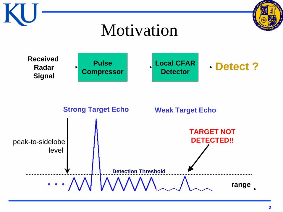
Motivation

Detection Threshold

Strong Target Echo Weak Target Echo

TARGET NOT DETECTED!!

PulseCompressor

Local CFARDetector

ReceivedRadarSignal

Detect ?

range• • •

peak-to-sidelobelevel

3

Adaptive Pulse Compression

• The Matched Filter is only matched to the transmitted signal, not the received signal.– Results in large target returns masking smaller nearby targets.

• Least Squares approaches have been proposed but they are not robust to “out-of-window” scatterers.– Degrade if there are scatterers in close proximity outside of

available data window.

• Employ Minimum Mean-Square Error (MMSE) estimation to adaptively estimate the filter that matches the return signal.– Denoted as Adaptive Pulse Compression.

4

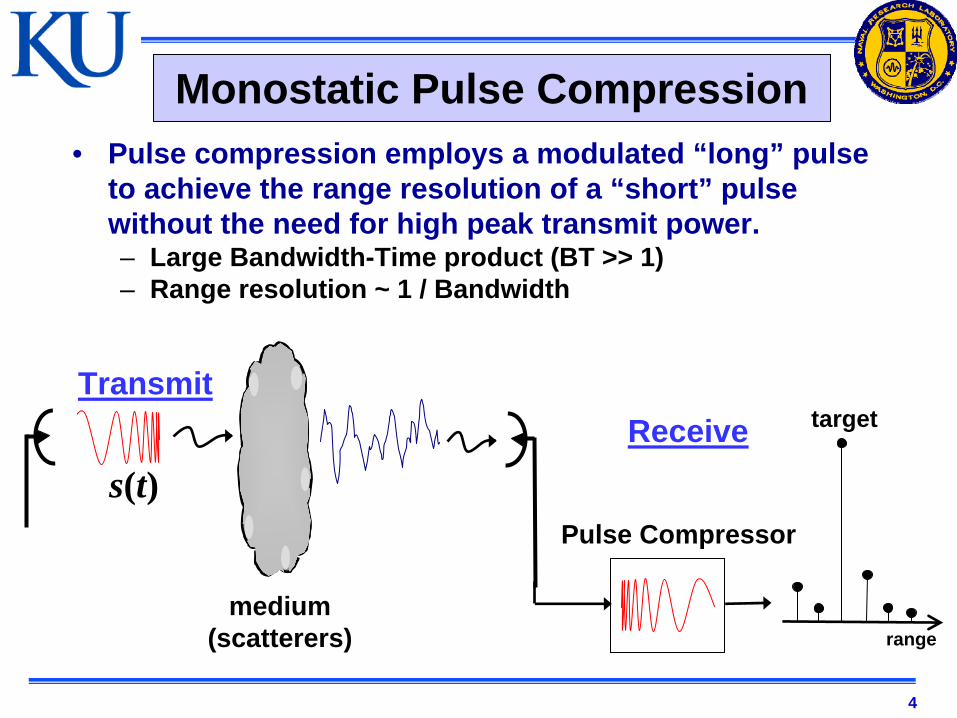
Monostatic Pulse Compression• Pulse compression employs a modulated “long” pulse

to achieve the range resolution of a “short” pulse without the need for high peak transmit power.– Large Bandwidth-Time product (BT >> 1)– Range resolution ~ 1 / Bandwidth

TransmitReceive

Pulse Compressor

rangemedium

(scatterers)

target

s(t)

5

Discrete System Model

s

x(ℓ)

Ground Truth Impulse Response

radar transmit signals ∗ x(ℓ)

received return signal

6

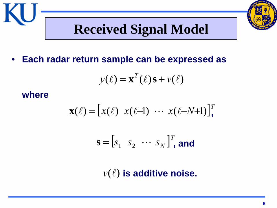
Received Signal Model

• Each radar return sample can be expressed as

where

,

, and

is additive noise.

)()()( vy T += sx

[ ]TNxxx )1()1()()( +−−=x

[ ]TNsss 21=s

)(v

7

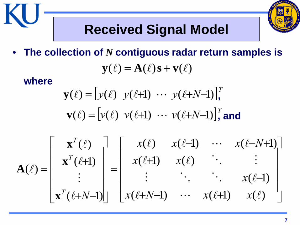
Received Signal Model• The collection of N contiguous radar return samples is

where ,

, and

)()()( vsAy +=

[ ]TNyyy )1()1()()( −++=y

[ ]TNvvv )1()1()()( −++=v

⎥⎥⎥⎥

⎦

⎤

⎢⎢⎢⎢

⎣

⎡

+−+−

++−−

=

⎥⎥⎥⎥⎥

⎦

⎤

⎢⎢⎢⎢⎢

⎣

⎡

−+

+=

)()1()1()1(

)()1()1()1()(

)1(

)1()(

)(

xxNxx

xxNxxx

NT

T

T

x

xx

A

8

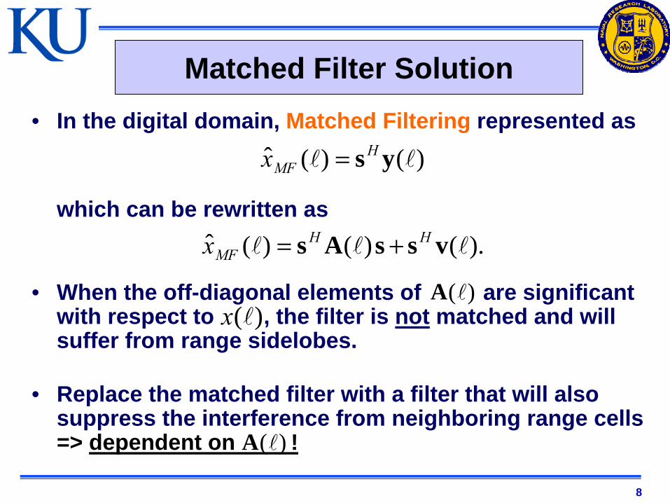
Matched Filter Solution• In the digital domain, Matched Filtering represented as

which can be rewritten as

• When the off-diagonal elements of are significant with respect to , the filter is not matched and will suffer from range sidelobes.

• Replace the matched filter with a filter that will also suppress the interference from neighboring range cells => dependent on !

)()(ˆ ysHMFx =

).()()(ˆ vssAs HHMFx +=

)(A

)(A

)(x

9

MMSE Formulation

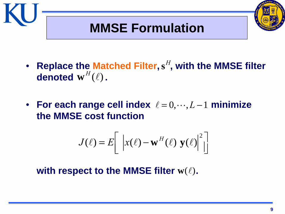
• Replace the Matched Filter, , with the MMSE filter denoted .

• For each range cell index minimize the MMSE cost function

with respect to the MMSE filter .

⎥⎦⎤

⎢⎣⎡ −=

2)()()()( yw HxEJ

Hs)(Hw

1,,0 −= L

)(w

10

MMSE Solution

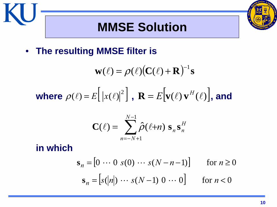
• The resulting MMSE filter is

where , , and

in which

( ) sRCw 1)()()( −+= ρ

[ ]2)()( xE=ρ [ ])()( HE vvR =

∑−

+−=

+=1

1

)(ˆ)(N

Nn

Hnnn ssC ρ

[ ] 0for)1()0(00 ≥−−= nnNssns

[ ] 0for00)1()( <−= nNsnsns

11

Implementation

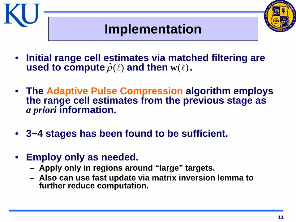
• Initial range cell estimates via matched filtering are used to compute and then .

• The Adaptive Pulse Compression algorithm employs the range cell estimates from the previous stage as a priori information.

• 3~4 stages has been found to be sufficient.

• Employ only as needed.– Apply only in regions around “large” targets.– Also can use fast update via matrix inversion lemma to

further reduce computation.

)(ρ̂ )(w

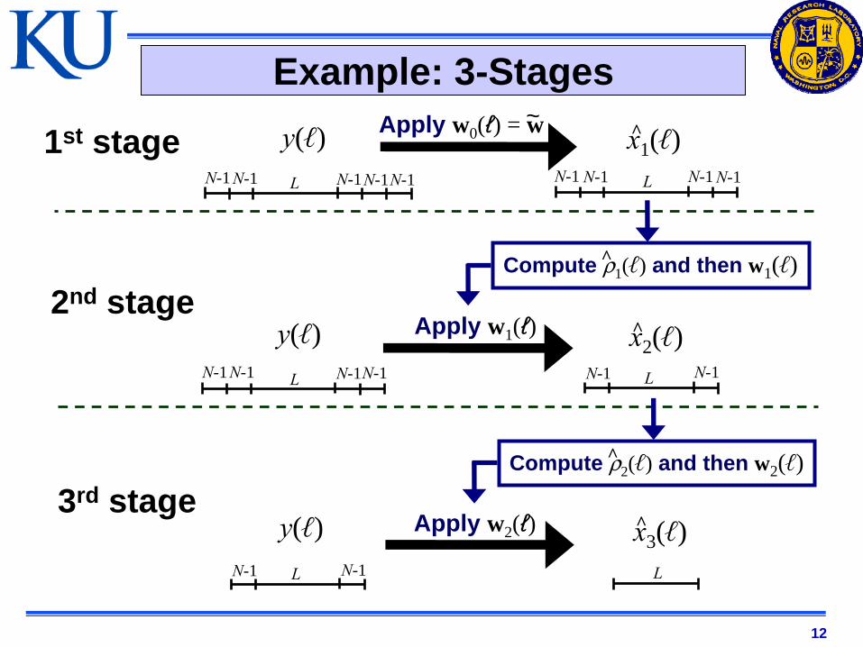
12

Example: 3-StagesApply w0(ℓ) = w

LN-1 N-1

y(ℓ)L

x3(ℓ)

1st stage

2nd stage

3rd stage

LN-1 N-1

y(ℓ)

LN-1 N-1

y(ℓ)

N-1N-1

N-1 N-1N-1 LN-1 N-1N-1 N-1

LN-1 N-1

x2(ℓ)

x1(ℓ)

Apply w1(ℓ)

Apply w2(ℓ)

~

Compute ρ2(ℓ) and then w2(ℓ)^

^

^

^

Compute ρ1(ℓ) and then w1(ℓ)^

13

Multistatic Interference Rejection

• Adaptive Pulse Compression is essentially an adaptive beamforming technique applied in the range domain.– For a given range cell, it puts a “range null” at relative

range offsets of nearby large targets.

• The approach can be generalized to accommodate multiple waveforms simultaneously (assuming the waveforms are known at the receiver).– Reject interference from other radars operating in-band

by “range nulling” large bi-static returns.

• May enable shared-spectrum radar to alleviate spectral crowding and provide additional capabilities.

14

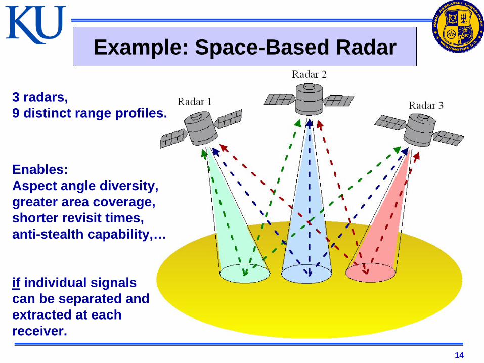
Example: Space-Based Radar

3 radars,9 distinct range profiles.

Enables:Aspect angle diversity,greater area coverage,shorter revisit times,anti-stealth capability,…

if individual signalscan be separated andextracted at each receiver.

15

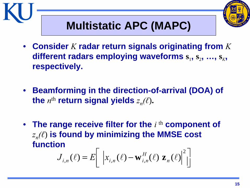
Multistatic APC (MAPC)

• Consider K radar return signals originating from Kdifferent radars employing waveforms s1, s2, …, sK, respectively.

• Beamforming in the direction-of-arrival (DOA) of the nth return signal yields zn(ℓ).

• The range receive filter for the i th component of zn(ℓ) is found by minimizing the MMSE cost function

⎥⎦⎤

⎢⎣⎡ −=

2

,,, )()()()( nH

ninini xEJ zw

16

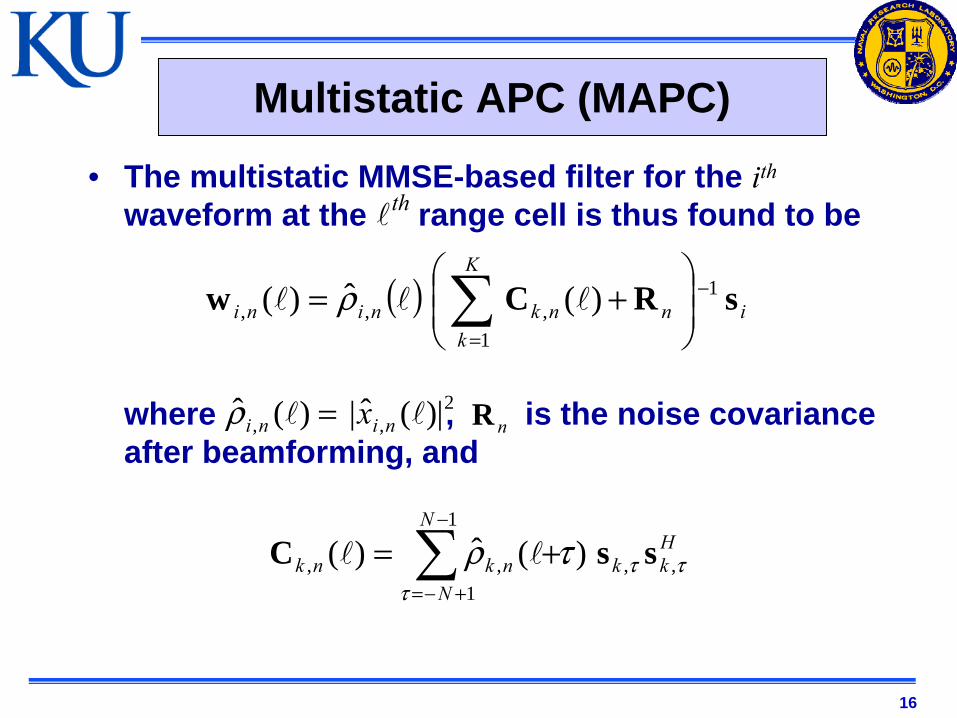
Multistatic APC (MAPC)

• The multistatic MMSE-based filter for the ith

waveform at the range cell is thus found to be

where , is the noise covariance after beamforming, and

2,, |)(ˆ|)(ˆ nini x=ρ nR

th

( ) in

K

knknini sRCw 1

1,,, )(ˆ)( −

=⎟⎟⎠

⎞⎜⎜⎝

⎛+= ∑ρ

∑−

+−=

+=1

1,,,, )(ˆ)(

N

N

Hkknknk

ττττρ ssC

17

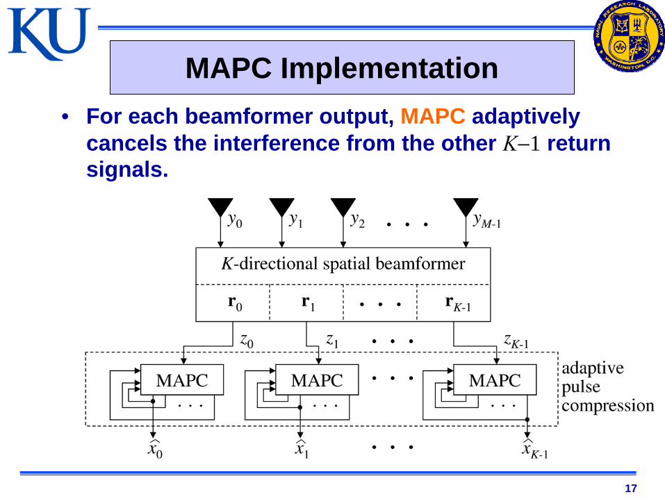
MAPC Implementation• For each beamformer output, MAPC adaptively

cancels the interference from the other K−1 return signals.

18

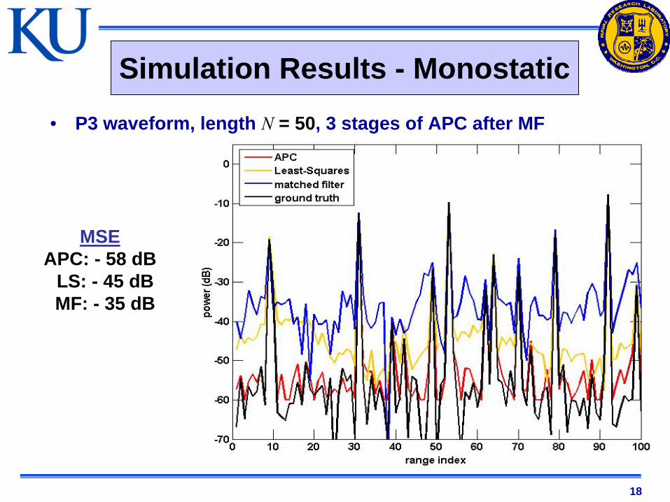
Simulation Results - Monostatic• P3 waveform, length N = 50, 3 stages of APC after MF

MSEAPC: - 58 dB

LS: - 45 dB MF: - 35 dB

19

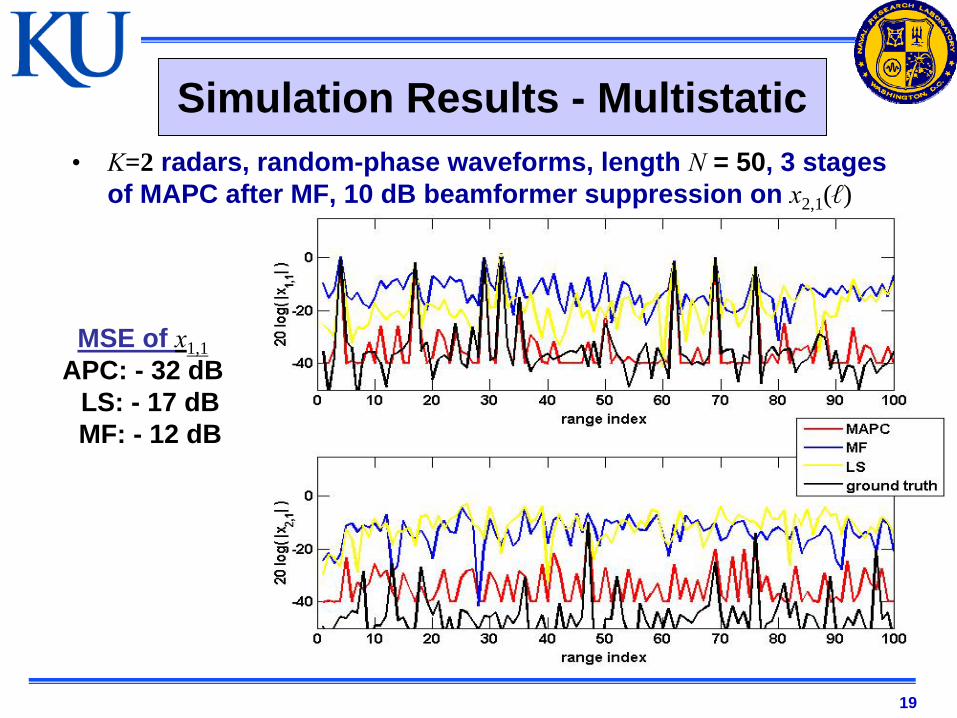
Simulation Results - Multistatic• K=2 radars, random-phase waveforms, length N = 50, 3 stages

of MAPC after MF, 10 dB beamformer suppression on x2,1(ℓ)

MSE of x1,1APC: - 32 dB

LS: - 17 dB MF: - 12 dB

20

Experimental Results

• Have begun experimental program at NRL to determine performance of APC/MAPC.

• Preliminary efforts to determine fidelity of waveform through portions of Tx/Rx chain.– Hi-fidelity waveform knowledge required for effective

cancellation performance.

Acknowledgement to Jean deGraaf and Aaron Shackelford of NRL for their efforts in collecting and analyzing the experimental data.

21

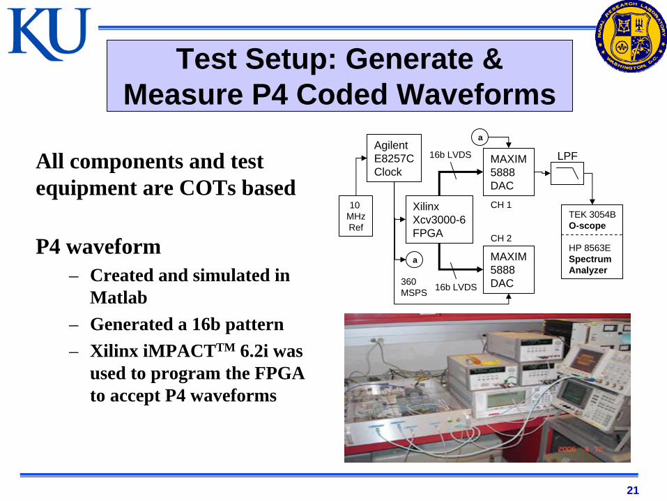
All components and test equipment are COTs based

P4 waveform– Created and simulated in

Matlab– Generated a 16b pattern– Xilinx iMPACTTM 6.2i was

used to program the FPGA to accept P4 waveforms

XilinxXcv3000-6FPGA

MAXIM5888DAC

MAXIM5888DAC

AgilentE8257CClock

10 MHzRef

360 MSPS

TEK 3054BO-scope

HP 8563ESpectrumAnalyzer

CH 1

CH 2

a

a

16b LVDS

16b LVDS

LPF

Test Setup: Generate & Measure P4 Coded Waveforms

22

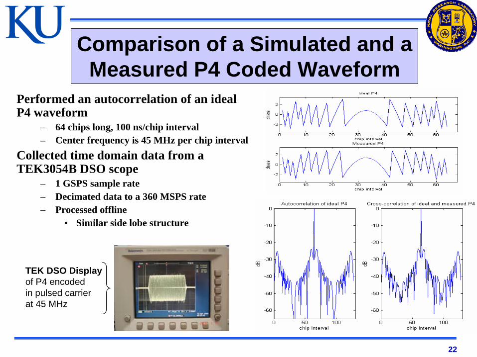
Performed an autocorrelation of an ideal P4 waveform

– 64 chips long, 100 ns/chip interval– Center frequency is 45 MHz per chip interval

Collected time domain data from a TEK3054B DSO scope

– 1 GSPS sample rate– Decimated data to a 360 MSPS rate– Processed offline

• Similar side lobe structure

TEK DSO Displayof P4 encodedin pulsed carrierat 45 MHz

Comparison of a Simulated and a Measured P4 Coded Waveform

23

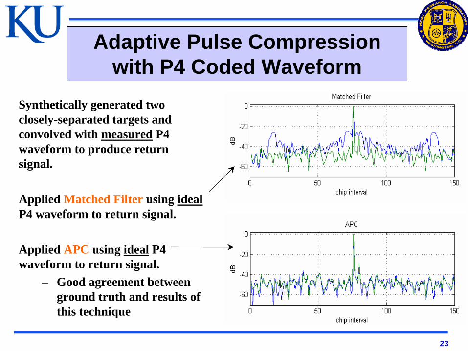
Synthetically generated two closely-separated targets and convolved with measured P4 waveform to produce return signal.

Applied Matched Filter using idealP4 waveform to return signal.

Applied APC using ideal P4 waveform to return signal.

– Good agreement between ground truth and results of this technique

Adaptive Pulse Compression with P4 Coded Waveform

24

Conclusions

• The Matched Filter is matched to the transmitted signal but not to the received signal which results in range sidelobes.

• The APC algorithm adaptively estimates the MMSE matched receive filter for each individual range cell in order to suppress range sidelobes.

• APC can be generalized to accommodate multiple received radar signals and may possibly facilitate shared-spectrum radar.

• Initial experimental results indicate that APC is robust to modest distortion of the transmission waveform. Further experimentation is underway to test the fidelity limits of the algorithm.