UNIVERSIDADE FEDERAL DO RIO GRANDE DO SULINSTITUTO DE INFORMÁTICA

PROGRAMA DE PÓS-GRADUAÇÃO EM COMPUTAÇÃO

GUSTAVO MELLO MACHADO

A Model for Simulation of Color VisionDe�ciency and A Color Contrast

Enhancement Technique for Dichromats

Thesis presented in partial fulfillmentof the requirements for the degree ofMaster of Computer Science

Prof. Dr. Manuel Menezes de Oliveira NetoAdvisor

Porto Alegre, September 2010

CIP – CATALOGING-IN-PUBLICATION

Machado, Gustavo Mello

A Model for Simulation of Color Vision Deficiency and AColor Contrast Enhancement Technique for Dichromats / GustavoMello Machado. – Porto Alegre: PPGC da UFRGS, 2010.

94 f.: il.

Thesis (Master) – Universidade Federal do Rio Grande do Sul.Programa de Pós-Graduação em Computação, Porto Alegre, BR–RS, 2010. Advisor: Manuel Menezes de Oliveira Neto.

1. Models of Color Vision. 2. Color Perception. 3. Simulationof Color Vision Deficiency. 4. Recoloring Algorithm. 5. Color-Contrast Enhancement. 6. Color Vision Deficiency. 7. Dichro-macy. 8. Anomalous Trichromacy. I. Oliveira Neto, ManuelMenezes de. II. Título.

UNIVERSIDADE FEDERAL DO RIO GRANDE DO SULReitor: Prof. Carlos Alexandre NettoVice-Reitor: Prof. Rui Vicente OppermannPró-Reitora de Pós-Graduação: Prof. Aldo Bolten LucionDiretor do Instituto de Informática: Prof. Flávio Rech WagnerCoordenador do PPGC: Prof. Álvaro Freitas MoreiraBibliotecária-Chefe do Instituto de Informática: Beatriz Regina Bastos Haro

“...Galega, tento descrever o que é estar com você...”— FRED ZERO QUATRO (MEU ESQUEMA)

ACKNOWLEGMENTS

I am deeply grateful to professor Manuel for his dedication as my advisor in this work,for the precision and lucidity of his teachings and suggestions that provided significanthelp to reach the outcomes, for his understanding and encouragement in times of difficultyand the severity in moments of weakness. With hard work and study, he introduced me tothe academic life, showed me a career and became an example of life.

I would also like to express my thanks to Leandro A. F. Fernandes who efficientlydrove the various experiments with volunteers and to the volunteers including my father.For all the moments of study and academic living, I thank my colleagues and professors,especially the ones from the Computer Graphics Group of PPGC-UFRGS.

I thank Giovane Kuhn for many fruitful discussions and suggestions, and FranciscoPinto for providing the visualization software. The many reference images used in thiswork were kindly provided by Francisco Pinto, CCSE at LBNL, Martin Falk e DanielWeiskopf, Karl Rasche and http://commons.wikimedia.org. This work was sponsored byCNPq-Brazil (grants 200284/2009-6, 131327/2008-9, 476954/2008-8, 305613/2007-3 and 142627/2007-0). Nvidia kindly donated the Quadro FX 5800 card used in thisresearch. I also thank the anonymous reviewers for their insightful comments on thesubmissions.

I would like to express special thanks to my wife, Sharon C. Andrade, for the mutuallove, for always supporting me, for her company that was fundamental to my effectiveparticipation in all stages of this work, and for accepting to be my “evolutionary part-ner” forever. I also thank my parents, Christiano H. L. Machado and Tereza M. MelloMachado, who were my advisors in life; my brother and sisters, Rodrigo, Denise andCamila, for the eternal friendship and trust; my mother-in-law Maria do Carmo Dias Cus-todio for her friendship and warm accommodation; and my grandmother, Lygia T. C.Mello, fan of Fluminense, for her love and for teaching me that we can lose everythingbut we must never lose the joke.

CONTENTS

LIST OF FIGURES . . . . . . . . . . . . . . . . . . . . . . . . . . . . . . . . 9

LIST OF TABLES . . . . . . . . . . . . . . . . . . . . . . . . . . . . . . . . 13

ABSTRACT . . . . . . . . . . . . . . . . . . . . . . . . . . . . . . . . . . . 15

RESUMO . . . . . . . . . . . . . . . . . . . . . . . . . . . . . . . . . . . . . 17

1 INTRODUCTION . . . . . . . . . . . . . . . . . . . . . . . . . . . . . . 191.1 Thesis Contributions . . . . . . . . . . . . . . . . . . . . . . . . . . . . . 211.2 Structure of the Thesis . . . . . . . . . . . . . . . . . . . . . . . . . . . . 21

2 BACKGROUND ON COLOR VISION DEFICIENCY . . . . . . . . . . . 232.1 Photoreceptor Cells . . . . . . . . . . . . . . . . . . . . . . . . . . . . . 232.2 Stage Theories of Human Color Vision . . . . . . . . . . . . . . . . . . . 242.3 Genetic of Human Photopigments . . . . . . . . . . . . . . . . . . . . . 252.4 Color Vision De�ciency . . . . . . . . . . . . . . . . . . . . . . . . . . . 25

3 RELATED WORK . . . . . . . . . . . . . . . . . . . . . . . . . . . . . . 293.1 Simulation Techniques . . . . . . . . . . . . . . . . . . . . . . . . . . . . 293.2 Recoloring Techniques . . . . . . . . . . . . . . . . . . . . . . . . . . . . 323.2.1 User-Assisted Techniques . . . . . . . . . . . . . . . . . . . . . . . . . . 323.2.2 Optimization-based Techniques . . . . . . . . . . . . . . . . . . . . . . . 323.2.3 Color-to-Grayscale Mappings . . . . . . . . . . . . . . . . . . . . . . . . 333.3 Summary . . . . . . . . . . . . . . . . . . . . . . . . . . . . . . . . . . . 35

4 A PHYSIOLOGICALLY-BASED MODEL FOR SIMULATION OF COLORVISION DEFICIENCY . . . . . . . . . . . . . . . . . . . . . . . . . . . . 37

4.1 Quanti�cation of The Stage Theory . . . . . . . . . . . . . . . . . . . . . 374.2 Simulating Color Vision De�ciency . . . . . . . . . . . . . . . . . . . . . 384.2.1 Simulating Anomalous Trichromacy . . . . . . . . . . . . . . . . . . . . 394.2.2 Simulating Dichromacy . . . . . . . . . . . . . . . . . . . . . . . . . . . 424.2.3 The Algorithm for Simulating CVD . . . . . . . . . . . . . . . . . . . . 454.3 Results . . . . . . . . . . . . . . . . . . . . . . . . . . . . . . . . . . . . . 464.3.1 Experimental Validation . . . . . . . . . . . . . . . . . . . . . . . . . . . 474.3.2 Discussion . . . . . . . . . . . . . . . . . . . . . . . . . . . . . . . . . . 504.4 Summary and Conclusions . . . . . . . . . . . . . . . . . . . . . . . . . 52

5 A REAL-TIME TEMPORAL-COHERENT COLOR CONTRAST ENHANCE-MENT FOR DICHROMATS . . . . . . . . . . . . . . . . . . . . . . . . . 55

5.1 The Color-Contrast Enhancing Technique . . . . . . . . . . . . . . . . . 565.1.1 Direction that Maximizes Contrast Loss . . . . . . . . . . . . . . . . . . 575.1.2 Computing the Final Colors . . . . . . . . . . . . . . . . . . . . . . . . . 585.1.3 Exaggerated Contrast . . . . . . . . . . . . . . . . . . . . . . . . . . . . 595.1.4 Enforcing Temporal Coherence . . . . . . . . . . . . . . . . . . . . . . . 595.2 Results . . . . . . . . . . . . . . . . . . . . . . . . . . . . . . . . . . . . . 595.2.1 Limitations . . . . . . . . . . . . . . . . . . . . . . . . . . . . . . . . . 635.3 Summary and Conclusions . . . . . . . . . . . . . . . . . . . . . . . . . 65

6 CONCLUSIONS AND FUTURE WORK . . . . . . . . . . . . . . . . . . 676.1 Future Work . . . . . . . . . . . . . . . . . . . . . . . . . . . . . . . . . 67

REFERENCES . . . . . . . . . . . . . . . . . . . . . . . . . . . . . . . . . . 69

APPENDIX A PRE-COMPUTED MATRICES FOR SIMULATION OF CVD 73

APPENDIX B EXPERIMENTAL DATA . . . . . . . . . . . . . . . . . . . . 75

APPENDIX C SIMULATION OF CVD USING SPD OF AN LCD . . . . . 79

APPENDIX D UM MODELO PARA SIMULAÇÃO DAS DEFICIÊNCIASNA PERCEPÇÃO DE CORES E UMA TÉCNICA DE AU-MENTO DO CONTRASTE DE CORES PARA DICROMÁ-TAS . . . . . . . . . . . . . . . . . . . . . . . . . . . . . . . 83

D.1 O Modelo para Simulação da Percepção de Cores . . . . . . . . . . . . . 85D.2 A Técnica de Realce de Contraste de Cores . . . . . . . . . . . . . . . . 88D.3 Conclusões . . . . . . . . . . . . . . . . . . . . . . . . . . . . . . . . . . 91

LIST OF FIGURES

Figure 1.1 (left) Europe’s map with colors used to encode the percentage of pop-ulation growth/decline of different countries in 2006. (right) simula-tion of deuteranopes’ perception of left image. . . . . . . . . . . . . 19

Figure 1.2 (left) the reference scientific visualization image (Brain dataset). (cen-ter) simulation of deuteranopes’ perception of left image. (right) sim-ulation of deuteranopes’ perception of recolored image. Simulationtechnique used for center and right images were the proposed by Bret-tel et al. and recoloring technique for right image was the proposedby Kuhn et al.. Reference image provided by Francisco Pinto. . . . . 20

Figure 2.1 Spectral sensitivity functions of the three cone types and the rods(after Smith and Pokorny) concerning an average normal trichromatindividual. These curves represent a ratio of probability of photoncapture as a function of wavelength. . . . . . . . . . . . . . . . . . . 24

Figure 2.2 Spectral response functions for the opponent channels concerning anaverage normal trichromat. . . . . . . . . . . . . . . . . . . . . . . . 25

Figure 2.3 Spectral sensitivity functions of cones in anomalous trichromats. Fig-ures from left to right refer to protanomaly, deuteranomaly, and tri-tanomaly, respectively. They illustrate the spectral shifts of anoma-lous cones, which occur in the three kinds of anomalous trichromacy. 26

Figure 2.4 Illustration simulating the perception of dichromats. (left) referenceimage (color wheel). The subsequent wheels refer from left to rightto the perception of protanopes, deuteranopes, and tritanopes, respec-tively. Wheels were simulated using Brettel et al.’s approach. . . . . 26

Figure 3.1 The three graphs illustrate the technique for simulating the percep-tion of individuals with dichromacy proposed by Brettel et al.. In theLMS color space, the original colors are orthographically projectedto corresponding semi-planes, along the direction defined by the axisrepresenting the affected cone. Illustrations of the technique for sim-ulating protanopia (left), deuteranopia (center), and tritanopia (right). 30

Figure 3.2 Examples showing the results obtained with Brettel et al.’s simula-tion technique. (a) a reference image showing a set of color pen-cils. The subsequent images show the simulation of the perception ofprotanopes (b), deuteranopes (c), and tritanopes (d). . . . . . . . . . . 31

Figure 3.3 Images demonstrating the simulation of the perception of Figure 3.2(left) by individuals with anomalous trichromacy according to theapproach proposed by Yang et al.. First row shows simulations ofprotanomalous’ perceptions while the second row shows simulationsof deuteranomalous’ perceptions. The four columns, from left toright, concerns anomalous trichromacy with severities (spectral shiftin wavelength) of 8 nm, 12 nm, 16 nm, and 20 nm, respectively. Tocompare with the perception of severe anomalous trichromacy, thelast column shows simulations according to Brettel et al.’s approachfor protanopes and deuteranopes in the first and second rows, respec-tively. . . . . . . . . . . . . . . . . . . . . . . . . . . . . . . . . . . 31

Figure 3.4 Demonstration of the results of two recently developed recoloringtechniques. (a) the reference image showing natural scene with someflowers in foreground. (b) simulation of the perception of individualswith deuteranopia according to Brettel et al.. Subsequently, simula-tions of deuteranope’s perception of the recolored images accordingto the approaches proposed by Rasche et al. in (c) and Kuhn et al. in(d). Images extracted from Kuhn et al.’s paper. . . . . . . . . . . . . 34

Figure 4.1 Scientific visualization under color vision deficiency. Simulation, fora normal trichromat, of the color perception of individuals with colorvision deficiency (protanomaly) at different degrees of severity. Theimage on the left (turbulent flows) illustrates the perception of a nor-mal trichromat and is used for reference. The numbers in parenthesisindicate the amount of shift, in nanometers, applied to the spectralresponse of the L cones. The image on the right shows the simu-lated perception of a dichromat (protanope), which is approximatelyequivalent to the perception of protanomalous with a spectral shiftof 20 nm. Note the progressive loss of color contrast as the degreeof severity increases. Images simulated using the proposed model.Reference image was provided by CCSE at LBNL. . . . . . . . . . . 38

Figure 4.2 Ingling and Tsou’s two-stage model of human color vision. The out-put of the photoreceptor stage (L, M and S cones) is linearly com-bined in the opponent stage (Vλ , y�b, and r�g nodes). . . . . . . . 39

Figure 4.3 (left) Cone spectral sensitivity functions for an average normal trichro-mat (after Smith and Pokorny). (right) Spectral response functions forthe opponent channels of the average normal trichromat according toIngling and Tsou’s model. These functions are obtained by evaluat-ing Equation 4.1 for the LMS triples resulting from the cone spectralsensitivity functions at all wavelengths in the visible range. . . . . . 40

Figure 4.4 Exon arrangements of the L, M, and hybrid photopigment genes. X-linked anomalous photopigment spectral sensitivity are interpreted asinterpolations of the normal L and M photopigment spectra. Adaptedfrom Sharpe et al.. . . . . . . . . . . . . . . . . . . . . . . . . . . . 40

Figure 4.5 Spectral opponent functions for anomalous trichromats. (left) Prot-anomaly (∆λL = 15 nm). (right) Deuteranomaly (∆λM = �19 nm).

. . . . . . . . . . . . . . . . . . . . . . . . . . . . . . . . . . . . . 41

Figure 4.6 Reference images. (a) Flower. (b) Brain. (c) Cat’s Eye nebula. (d)Scatter plot. (e) Slice of the HSV color space (V=1). (f) Tornado. . . 43

Figure 4.7 Simulation of dichromatic perception for the flower shown in Fig-ure 4.6(a) according to four different models. From left to right:empty space / empty cones, photopigment substitution (replacementmodel), photopigment substitution with scaling according to Equa-tion 4.15, same as previous but also scaled by 0.96, Brettel et al.’s(for reference). . . . . . . . . . . . . . . . . . . . . . . . . . . . . . 43

Figure 4.8 Comparison of the plausible dichromacy models considering the en-tire RGB space (protanopia case). A surface obtained using Brettelet al.’s algorithm is shown for reference in all images. (a) EmptySpace / Empty Cones model. (b) Replacement model. (c) Replace-ment model using Equation 4.15. (d) Same as (c) but also scaled by0.96. . . . . . . . . . . . . . . . . . . . . . . . . . . . . . . . . . . 45

Figure 4.9 Simulation of protanomalous and deuteranomalous vision for severaldegrees of severity (expressed in nm). Last column: result of Brettelet al.’s algorithm for reference. P/D (Model): Protanomaly/Deuter-anomaly simulated with the proposed technique. P/D (Yang): Prot-anomaly/Deuteranomaly simulated with Yang et al.’s technique. . . . 48

Figure 4.10 Simulation of protanomalous and deuteranomalous vision in scien-tific visualization. From top to bottom: brain dataset, Tornado, Scat-ter plot, and Cat’s Eye nebula. The degrees of severity are expressedin nm. Last column: Brettel et al.’s dichromatic simulation for refer-ence. Pnomaly: Protanomaly. Dnomaly: Deuteranomaly. . . . . . . . 49

Figure 4.11 Averaged results of the Farnsworth-Munsell 100H test performed by17 normal trichromats using the test original colors. . . . . . . . . . . 50

Figure 4.12 Averaged results of the Farnsworth-Munsell 100H test. (a) Normaltrichromats simulating protan vision. (b) Protan results for the orig-inal colors. (c) Normal trichromats simulating deutan vision. (d)Deutan results for the original colors. . . . . . . . . . . . . . . . . . 51

Figure 4.13 Visualization of the Visible Male’s head using the same transfer func-tion (bottom) defined over the color gamut (top row) of a normaltrichromat, a protanomalous (10 nm), and a protanope. . . . . . . . . 52

Figure 5.1 Comparison of the results produced by the proposed recoloring tech-nique and by Kuhn et al.’s for a set of scientific visualization images.The "Dichromat" column shows the simulated perception of dichro-mats for the corresponding "Reference" image obtained using the ap-proach presented in Chapter 4 The simulation and recolorings of theFlame and Nebula images are for deuteranopes, while the Tornadoones are for protanopes. . . . . . . . . . . . . . . . . . . . . . . . . 56

Figure 5.2 Planar approximation for the color gamut of dichromats in the CIEL�a�b� color space. (a) Protanope (θp = �11.48�). (b) Deuteranope(θd =�8.11�). (c) Tritanope (θt = 46.37�). . . . . . . . . . . . . . 57

Figure 5.3 The steps of the proposed recoloring algorithm. (a) Colors c1 to c4are perceived by a dichromat as c01 to c04, respectively (their projec-tions on the dichromat’s gamut plane). The relative loss of contrastexperienced by a dichromat for a pair of colors (ci,c j) is given byl(ci,c j) = (kci�c jk�kc0i�c0jk)/(kci�c jk), which happens along thedirection ϑi j = ci� c j. (b) Direction vab (shown in blue) that maxi-mizes the loss of local contrast (in a least-square sense) is computedas the main eigenvector of the matrix MT M, where M is defined inEquation 5.2. (c) Projection of the original colors on the plane definedby vab and L�. (d) Final colors obtained after rotating the projectedcolors c00k in (c) around L� so that they align with the dichromat’splane. . . . . . . . . . . . . . . . . . . . . . . . . . . . . . . . . . . 58

Figure 5.4 Comparison of the results produced by the proposed technique andby Kuhn et al.’s. First row, from left to right: reference image, simu-lated perception of a deuteranope, and recolored images using variousalgorithms. Second row: Perceptual errors according to the DRIMmetric. Third row: Local contrast differences according to the RMSmetric of Equation 5.3 (for k = 100). According to both metrics, theproposed recoloring technique is less prone to noticeable changes incontrast. . . . . . . . . . . . . . . . . . . . . . . . . . . . . . . . . . 60

Figure 5.5 Recoloring of information visualization images for protanopes. . . . 61Figure 5.6 Integration of the proposed technique with an existing visualization

application. (left) Reference image as perceived by an individual withnormal color vision. (center) Simulation of the perception of a deuter-anope for the reference image using the model explained in chapter 4.(right) Recolored image for a deuteranope using the proposed tech-nique. . . . . . . . . . . . . . . . . . . . . . . . . . . . . . . . . . . 61

Figure 5.7 Example of a situation that causes the proposed technique to fail.Note that deuteranopes (and protanopes) already perceive the refer-ence image as having sufficient contrast, and no recoloring is neces-sary. . . . . . . . . . . . . . . . . . . . . . . . . . . . . . . . . . . 63

Figure 5.8 Comparison of the results produced by the proposed technique andthe ones obtained with Kuhn et al.’s approach for a set of medicalvisualization images. The even rows show the estimated changes incontrast perceived by an observer in the recolored images (with re-spect to the reference images), according to the DRIM metric. Greenindicates loss of contrast, blue represents contrast ampli�cation, andred shows regions with contrast reversal. The metric favors the pro-posed technique’s results in all examples. Reference images Kneeand Foot were provided by Francisco Pinto. . . . . . . . . . . . . . . 64

LIST OF TABLES

Table 1.1 Incidence of red-green color blindness among different ethnic groups. 20

Table 2.1 Incidence of CVD types among Caucasian population. . . . . . . . . 27

Table 5.1 Performance comparison (in sec.) of the proposed technique andKuhn et al.’s for both CPU and GPU versions of the algorithms ex-ecuted on several images. Due to the linear cost of the proposedapproach, the relative speedup improves as the image size increases. . 62

Table 5.2 Times (in sec.) for the quantization and reconstruction phases of thetechnique of Kuhn et al. for several images. K-means used in theCPU version of the technique, and uniform quantization used in itsGPU version. The column Clusters shows the number of clustersidentified in the quantization phase. . . . . . . . . . . . . . . . . . . 63

ABSTRACT

Color vision deficiency (CVD) affects approximately 200 million people worldwide,compromising the ability of these individuals to effectively perform color and visualization-related tasks. This has a significant impact on their private and professional lives.

This thesis presents a physiologically-based model for simulating color perception.Besides modeling normal color vision, it also accounts for the hereditary and most preva-lent cases of color vision deficiency (i.e., protanopia, deuteranopia, protanomaly, anddeuteranomaly), which together account for approximately 99.96% of all CVD cases.This model is based on the stage theory of human color vision and is derived from datareported in electrophysiological studies. It is the first model to consistently handle nor-mal color vision, anomalous trichromacy, and dichromacy in a unified way. The proposedmodel was validated through an experimental evaluation involving groups of color visiondeficient individuals and normal color vision ones. This model can provide insights andfeedback on how to improve visualization experiences for individuals with CVD. It alsoprovides a framework for testing hypotheses about some aspects of the retinal photore-ceptors in color vision deficient individuals.

This thesis also presents an automatic image-recoloring technique for enhancing colorcontrast for dichromats whose computational cost varies linearly with the number of inputpixels. This approach can be efficiently implemented on GPUs, and for typical imagesizes it is up to two orders of magnitude faster than the current state-of-the-art technique.Unlike previous approaches, the proposed technique preserves temporal coherence and,therefore, is suitable for video recoloring. This thesis demonstrates the effectiveness ofthe proposed technique by integrating it into a visualization system and showing, for thefirst time, real-time high-quality recolored visualizations for dichromats.

Keywords: Models of Color Vision, Color Perception, Simulation of Color Vision De-ficiency, Recoloring Algorithm, Color-Contrast Enhancement, Color Vision Deficiency,Dichromacy, Anomalous Trichromacy.

RESUMO

Um Modelo para Simulação das De�ciências na Percepção de Cores e Uma Técnicade Aumento do Contraste de Cores para Dicromátas

As Deficiências na Percepção de Cores (DPC) afetam aproximadamente 200 milhõesde pessoas em todo o mundo, comprometendo suas habilidades para efetivamente realizartarefas relacionadas com cores e com visualização. Isto impacta significantemente osâmbitos pessoais e profissionais de suas vidas.

Este trabalho apresenta um modelo baseado na fisiologia para simulação da percep-ção de cores. Além de modelar visão de cores normal, ele também compreende os ti-pos mais predominantes de deficiências na visão de cores (i.e., protanopia, deuteranopia,protanomalia e deuteranomalia), cujas causas são hereditárias. Juntos estes representamaproximadamente 99.96% de todos os casos de DPC. Para modelar a percepção de coresda visão humana, este modelo é baseado na teoria dos estágios e é derivado de dados re-portados em estudos eletrofisiológicos. Ele é o primeiro modelo a consistentemente tratarvisão de cores normal, tricromacia anômala e dicromacia de modo unificados. Seus re-sultados foram validados por avaliações experimentais envolvendo grupos de indivíduoscom deficiência na percepção de cores e outros com visão de cores normal. Além disso,ele pode proporcionar a melhor compreensão e um feedback sobre como aperfeiçoar asexperiências de visualização por indivíduos com DPC. Ele também proporciona um fra-mework para se testar hipóteses sobre alguns aspectos acerca das células fotoreceptorasna retina de indivíduos com deficiência na percepção de cores.

Este trabalho também apresenta uma técnica automática de recoloração de imagensque visa realçar o contraste de cores para indivíduos dicromatas com custo computacio-nal variando linearmente com o número de pixels. O algoritmo proposto pode ser efici-entemente implementado em GPUs, e para imagens com tamanhos tipicos ele apresentaperformance de até duas ordens de magnitude mais rápida do que as técnicas estado daarte atuais. Ao contrário das abordagens anteriores, a técnica proposta preserva coerênciatemporal e, portanto, é adequado para recoloração de vídeos. Este trabalho demonstra aefetividade da técnica proposta ao integrá-la a um sistema de visualização e apresentando,pela primeira vez, cenas de visualização recoloridas para dicromatas em tempo-real e comalta qualidade.

Palavras-chave: Modelos da Visão de Cores, Percepção de Cores, Simulação de Defi-ciências na Percepção de Cores, Algorítimo de Recoloração, Aumento de Contraste deCores, Deficiências na Percepção de Cores, Dicromacia, Tricromacia Anômala.

19

1 INTRODUCTION

Color Vision De�ciency (CVD) affects one’s ability to distinguish between certaincolors. Such condition is predominantly caused by hereditary reasons, while, in somerare cases, it is believed to be acquired by neurological injuries. Estimates indicate thatabout two hundred million people worldwide have some kind of CVD. Furthermore, thereis no known treatment or cure for these dysfunctions.

Individuals with CVD have difficulties in performing color related tasks, which inter-feres with their personal and professional lives. For example, the map shown in Figure 1.1(left) aims to illustrate population growth/decline in Europe’s countries in 2006 using col-ors, whose contrast allows the correlation between percentage ranges and countries. Suchcombination of colors seems to be reasonable to represent the data when the map is readby individuals with normal color vision. But, for individuals with deuteranopia1, the col-ors representing population growth of up to 0.5% and population decline of up to 0.5%are indistinguishable (Figure 1.1 right). This example demonstrates a recurring situationin information visualization and scientific visualization images.

Figure 1.1: (left) Europe’s map with colors used to encode the percentage of populationgrowth/decline of different countries in 2006. (right) simulation of deuteranopes’ percep-tion of left image. Left image is from (WIKIMEDIA COMMONS, 2010).

Red-green color vision de�ciency comprises the most common types of CVD (approx-imately 99.96% of all cases), which are characterized by malfunction of L- or M-conesopsins. Such opsins are encoded by genes located on the X chromosome. Thus, such types

1Deuteranopia is a CVD type characterized by the absence of M-photopigments in retina.

20

are caused by X-linked inheritance and are more prevailing among the male population.Table 1.1 shows the incidence of red-green CVD among different ethnic groups.

Ethnic Groups Incidence of red-green CVD (%)Male Female

Caucasians 7.9 0.42Asians 4.2 0.58Africans 2.6 0.54

Table 1.1: Incidence of red-green color blindness among different ethnic groups (RIG-DEN, 1999; SHARPE et al., 1999).

The most relevant works dealing with CVD can be broadly classified as techniquesfor simulation and recoloring. The first group aims to provide tools for demonstrating forindividuals with normal color vision how some color stimuli are perceived by individualswith CVD. Such tools help to better understand the difficulties faced by these individuals.Moreover, they can provide insights and feedback, for example, on how to improve visu-alization experiences for individuals with color vision deficiency. Recoloring algorithms,on the other hand, aim to change image colors so that individuals with CVD can recover(as much as possible) the lost color contrast. No previous techniques are capable to pro-vide real-time recoloring. Besides, an efficient technique could be integrated to portabledevices, which would impact these individuals’ daily lives.

The results of state-of-art techniques for simulation and recoloring are illustrated inFigure 1.2. It uses as reference (Figure 1.2 left) a scientific visualization image. Fig-ure 1.2 (center) shows the simulation of deuteranopes’ perception for the reference imageaccording to Brettel et al. (BRETTEL; VIÉNOT; MOLLON, 1997). For these individu-als, the ability to distinguish between certain colors vanishes compromising their capacityto identify the image features. Note, however, how a recoloring technique (Figure 1.2right) offers a good possibility for these individuals to perceive the contrasts. This imagewas recolored according to the exaggerated approach proposed by Kuhn et al. (KUHN;OLIVEIRA; FERNANDES, 2008a), which preserves image naturalness.

Figure 1.2: (left) the reference scientific visualization image (Brain dataset). (center)simulation of deuteranopes’ perception of left image. (right) simulation of deuteranopes’perception of recolored image. Simulation technique used for center and right imageswere the proposed by Brettel et al. (BRETTEL; VIÉNOT; MOLLON, 1997) and recol-oring technique for right image was the proposed by Kuhn et al. (KUHN; OLIVEIRA;FERNANDES, 2008a). Reference image provided by Francisco Pinto.

21

1.1 Thesis Contributions

This thesis presents two novel techniques (i.e., a simulation and a recoloring) to solvethe main limitations of the state-of-art techniques. Both techniques were successfully in-tegrated into a visualization system, which allowed the practical validation of its results.Both works were published in visualization journals (MACHADO; OLIVEIRA; FER-NANDES, 2009; MACHADO; OLIVEIRA, 2010). The simulation technique introducedin this thesis presents the following contributions:

� First model that consistently simulates normal trichromacy, dichromacy2, and anoma-lous trichromacy3 while previous model addressed only dichromacy.� A single model for simulation that comprises about 99.96% of all cases of CVD

while previous approaches addressed only 27.46% of the cases.

And the recoloring technique presented in this thesis has the following contributions:

� High-quality results comparable to results obtained with the state-of-art technique.� Real-time recoloring. Performance of up to two orders of magnitude faster than the

state-of-art technique.� Temporal coherence preservation, not requiring prior knowledge of subsequent

frames.

1.2 Structure of the Thesis

This dissertation is organized as follows: Chapter 2 introduces the color vision de-ficiencies by addressing the concepts and theories of color perception in humans andprovides some useful terminologies. Chapter 3 describes the related works emphasizingthe most relevant ones to this thesis. It introduces the state-of-art techniques among sim-ulation and recoloring approaches. Besides, it presents some relevant color-to-grayscaletechniques, as they represent algorithms involving dimensionality reduction, a techniqueakin to recoloring techniques for dichromats. Chapter 4 presents a physiologically-basedmodel for simulation of the perception of individuals with CVD. Moreover, it explainshow this model is supported by known theories of color perception and knowledge aboutcolor vision deficiencies. It also compares its results with the state-of-art simulationtechniques and describes an experiment used to validate the proposed model. Chapter 5presents a recoloring algorithm that can produce high-quality results in real-time, as wellas temporal coherence. It compares its results with the state-of-art recoloring techniqueand shows the benchmark results, that validated the techniques performance. Moreover,it demonstrates the successful integration with a visualization system. Finally, Chapter 6concludes the thesis and suggests some possibilities of future work.

2Dichromacy is a CVD type characterized by absence of one type of photopigment in the human retina.3Anomalous trichromacy is a CVD type characterized by an abnormal cone type in the retina.

22

23

2 BACKGROUND ON COLOR VISION DEFICIENCY

This chapter reviews the concepts involving color vision deficiency. It provides somebackground for the techniques presented in this thesis and summarizes the theories andfundamentals of color perception. Finally, it explains details about each type of CVD,emphasizing the most relevant ones.

2.1 Photoreceptor Cells

Photoreceptor cells are present in the retina and are characterized for being sensitiveto light. Their sensitivities are defined by spectral absorption functions, which depend onthe photopigment type contained. In the human retina, these cells are broadly classifiedas cones and rods.

The rods are primarily responsible for night vision, i.e., low light environment sight.The photopigment type contained in the rods is called rhodopsin1. This name concernsthe red color reflected by the pigment, while the color absorbed by it corresponds mainlyto regions of the spectrum with bluish tones. But the rods do not contribute to colorperception in humans except under special conditions (SHARPE et al., 1999).

Cones are the photoreceptors responsible for color perception in humans. They act pri-marily in highly-illuminated environments. Cones are classified as L, M, and S, dependingon their sensitivity to the spectrum regions with Long, Medium, and Short wavelengths,respectively.

The spectral sensitivity functions of the four photoreceptors types (i.e., the three conetypes and the rods) concerning an average normal trichromat individual are illustratedthrough the curves in Figure 2.1. These functions are usually graphically represented forease of reading while define a relationship between probability of photons capture and thewavelength (SHARPE et al., 1999).

Spectral sensitivity functions associated to the L, M, and S cones overlap each otherfor some wavelength ranges, as can be noticed in Figure 2.1. This is more relevant forthe L- and M-cones. Actually, a photoreceptor is only able to measure the total amountof incident light, responding according to its sensitivity function. For instance, two hy-pothetical radiations with 600 nm and 500 nm separately will result in equivalent stimulito M cones, since its sensitivities to both wavelengths are approximately equal. Thus,the human visual system will distinguish between these two radiations by combining theresponses of the three cone types.

1Rhodopsin: from Greek, Rhodo means red and Opsin means sight.

24

Figure 2.1: Spectral sensitivity functions of the three cone types and the rods (after Smithand Pokorny (SMITH; POKORNY, 1975)) concerning an average normal trichromat in-dividual. These curves represent a ratio of probability of photon capture as a function ofwavelength (SHARPE et al., 1999).

2.2 Stage Theories of Human Color Vision

There are some theories about how cone cells sensitivity are interpreted as colors bythe human visual system. The trichromatic theory of color vision assumes the existenceof three kinds of photoreceptors (cone types) with different spectral sensitivities. Theresponses produced by these photoreceptors would then be sent to the central nervoussystem and perceived as color sensations (WYSZECKI; STILES, 2000). Also knownas the Young-Helmholtz three-component theory, it is based on the analysis of the stimulirequired to evoke color sensations and provides satisfactory explanation for additive color-matching experiments.

Unfortunately, the theory cannot explain some perceptual issues, such as the opponentnature of visual afterimages, as well as why some hues are never perceived together whileothers (e.g., green and yellow, green and blue, red and yellow, and red and blue) are easilyfound (FAIRCHILD, 1997). All these effects can be satisfactorily explained by Hering’sopponent-color theory, which assumes the existence of six basic colors (white, black,red, green, yellow, and blue). According to Hering, light is absorbed by photopigmentsbut, instead of having six separate channels, the visual system uses only three opposingchannels: white-black (WS), red-green (RG), and yellow-blue (Y B). While equal amountsof black and white produce a gray sensation, equal amounts of yellow and blue cancel tozero. Likewise, equal amounts of red and green also cancel out. Zero in this contextmeans that the spectral response functions for the opponent channels (Figure 2.2) becomezero at the points where opponent colors take equal values.

Considered separately, neither the trichromatic theory nor the opponent-color theorysatisfactorily explains several important color-vision phenomena. When combined, how-ever, they could explain and predict many color vision phenomena involving color match-ing, color discrimination, color appearance, and chromatic adaptation, among others, forboth normal color vision and color vision deficient observers (WYSZECKI; STILES,2000). von Kries suggested that the trichromatic theory should be valid at the photore-ceptor level, but the resulting signals should be further processed in a later stage accordingto the opponent-color theory (JUDD, 1966). This so-called stage theory (also known aszone theory) provides the best models for human color vision. Besides the two-stage the-

25

Figure 2.2: Spectral response functions for the opponent channels concerning an averagenormal trichromat.

ory suggested by von Kries, other two- and three-stage theories of color vision have beenproposed, including Müller three-stage theory. A discussion of some of these theories canbe found in (JUDD, 1966).

2.3 Genetic of Human Photopigments

Besides being closely located in the X chromosome, exons2 concerning both L- andM-cones photopigments are similarly encoded. Actually, anomalous combinations ofthese exons are supposed to be responsible for all cases of red-green color vision defi-ciencies. Explanations for all these similarities can be supported by the evolution of opsingenes as described in (SHARPE et al., 1999). The L- and M-cones photopigments arevery similar. They were the last to emerge throughout the evolutionary process of humancolor vision. About the evolution of genes responsible for production of rhodopsin, con-tained in the rods, little is known. It is believed that it has evolved from the S-opsin gene,but it is known that in humans it is located on chromosome 3 (SHARPE et al., 1999).

2.4 Color Vision De�ciency

Color vision deficiencies are broadly classified as anomalous trichromacy, dichro-macy and monochromacy. Anomalous trichromacy is characterized by the presence inretina of one anomalous cone type. The anomalous cone contains a different photopig-ment type which spectrally deviates the cone’s sensitivity. Anomalous trichromacy isfurther classified as protanomaly, deuteranomaly and tritanomaly3 depending on whetherthe anomalous are the L, M, or S cones, respectively. In these cases, the sensitivitiesof the anomalous cones are shifted to different bands of the spectrum. Figure 2.3 illus-trates these shifts for the three kinds of anomalous trichromacy. In cases of protanomaly(Figure 2.3 left), the sensitivities of the anomalous L cones are much similar to that ofnormal M cones, as it is shifted toward shorter wavelengths spectrum bands. Sensitiv-ity functions of anomalous M cones in deuteranomalous (Figure 2.3 center) resemble thesensitivity functions of normal L cones, as they are shifted toward longer wavelengths.

2Exon is an active sequence of genes, i.e., it encodes information for protein synthesis.3Prot, Deut, and Trit prefixes origins from Greek meaning One, Two and Three, respectively. These

prefixes refers to L, M, and S cones, respectively.

26

The cases of tritanomaly are very rare, and the S-cones sensitivities are shifted towardlonger wavelengths (Figure 2.3 right).

Figure 2.3: Spectral sensitivity functions of cones in anomalous trichromats. Figures fromleft to right refer to protanomaly, deuteranomaly, and tritanomaly, respectively. They il-lustrate the spectral shifts of anomalous cones, which occur in the three kinds of anoma-lous trichromacy.

In dichromatic retina there are only two types of photopigments. Dichromacy is fur-ther classified as protanopia, deuteranopia, and tritanopia, depending on whether the ab-sent photopigment concerns the L-, M-, or S-cone type, respectively. The perceived colorsby individuals with both protanopia and deuteranopia are similar. As reported by unilat-eral dichromats4, protanopes and deuteranopes can only experience yellowish and blueishhues including gray shades (MEYER; GREENBERG, 1988; BRETTEL; VIÉNOT; MOL-LON, 1997; VIÉNOT; BRETTEL; MOLLON, 1999). For tritanopia, a much rarer condi-tion, individuals will always experience colors between a blueish-green and a reddish hue.Figure 2.4 illustrates the colors experienced by the three types of dichromacy. Figure 2.4(left) shows a color wheel which is used as reference. The three subsequent images illus-trate from left to right, the perception of the reference image by protanopes, deuteranopes,and tritanopes, respectively. Note how their color gamuts are reduced if compared to thegamut of individuals with normal color vision.

Figure 2.4: Illustration simulating the perception of dichromats. (left) reference im-age (color wheel). The subsequent wheels refer from left to right to the perception ofprotanopes, deuteranopes, and tritanopes, respectively. Wheels were simulated usingBrettel et al.’s approach (BRETTEL; VIÉNOT; MOLLON, 1997).

The cases of monochromacy are classified as rod-monochromacy, when there are nocones in the retina; and cone-monochromacy, when there is only one cone type in theretina. Monochromacy cases are very rare and are not treated in this thesis.

4Unilateral dichromats are individuals with dichromacy in only one eye while the other has normal colorvision.

27

CVD Type Incidence (%)Male Female

Anomalous trichromacy 5.71 0.39Protanomaly 1.08 0.03Deuteranomaly 4.63 0.36Tritanomaly 0.0001 0.0001Dichromacy 2.28 0.03Protanopia 1.01 0.02Deuteranopia 1.27 0.01Tritanopia 0.002 0.001Monochromacy 0.003 0.00001

Table 2.1: Incidence of CVD types among Caucasian population (RIGDEN, 1999;SHARPE et al., 1999).

The incidences of the CVD types among the caucasian population, which is the onlyethnic group for which there are some reliable statistics available, are shown in Ta-ble 2.1. Note that red-green color vision deficiencies (comprising protanopia, deutera-nopia, and protanomaly deuteranomaly) are more prevailing while tritanopia, tritanomaly,and monochromacy are very rare.

28

29

3 RELATED WORK

This chapter describes the most relevant works on simulation and recoloring for colorvision deficiency, emphasizing their strenghs and limitations. Some works in color-to-grayscale conversion are also discussed in this chapter, since they deal with dimensional-ity reduction, and, as such, are akin to recoloring algorithms for dichromats.

3.1 Simulation Techniques

Despite the relevance of understanding how individuals with CVD perceive colors, lit-tle work has been done in simulating their perception for normal trichromats. In particular,none of the previous approaches is capable of handling both dichromacy and anomaloustrichromacy while the simulation technique proposed in this thesis does. One should alsonote that the simulation process is not symmetrical: in general, it is not possible to simu-late a normal trichromatic color experience for individuals with CVD, due to the reducedcolor gamuts of deficient color vision systems.

The first techniques that simulates the perception of individuals with CVD were de-veloped based on the report of unilateral dichromat individuals. According to their re-port (GRAHAM; HSIA, 1959; JUDD, 1949a; SLOAN; WOLLACH, 1948) achromaticcolors as well as some other hues are perceived similarly by both eyes (approximatelywavelengths of 475 nm and 575 nm by individuals with protanopia and deuteranopia,and 485 nm and 660 nm by tritanopes). Meyer and Greenberg (MEYER; GREENBERG,1988) mapped this gamut in the XYZ color space. They also mapped confusion lines inthis color space, which represent directions along which there is no color variation ac-cording to dichromats perception. By projecting colors through confusion lines into thereduced gamut, they defined an accurate technique for simulating dichromacy.

Latter, some other similar works have been developed (BRETTEL; VIÉNOT; MOL-LON, 1997; VIÉNOT; BRETTEL; MOLLON, 1999). The technique proposed by Brettelet al. (BRETTEL; VIÉNOT; MOLLON, 1997) is the most referenced of all existing sim-ulation techniques. In this technique, the color gamut of dichromats is mapped to twosemi-planes in the LMS color space, while the authors constrained the direction of con-fusion lines to be parallel to the direction of the color space axes L, M, or S, dependingon whether the dichromacy type is protanopia, deuteranopia, or tritanopia, respectively.Figure 3.1 illustrates the process of projecting colors onto the semi-planes. For exam-ple, when simulating deuteranopia (Figure 3.1 center) the colors are projected onto thesemi-planes through the direction of the M axis. This process is analogous for protanopia(Figures 3.1 left) and tritanopia (Figures 3.1 right). Figure 3.2 shows examples of some re-sults of this simulation technique using Figure 3.2 (a) as reference image. Figures 3.2 (b),(c), and (d) shows the simulation of the perception of protanopes, deuteranopes, and tri-

30

tanopes, respectively. Note how the perception of color contrasts vanishes for some huesin different types of dichromacy.

Figure 3.1: The three graphs illustrate the technique for simulating the perception of in-dividuals with dichromacy proposed by Brettel et al. (BRETTEL; VIÉNOT; MOLLON,1997). In the LMS color space, the original colors are orthographically projected to cor-responding semi-planes, along the direction defined by the axis representing the affectedcone. Illustrations of the technique for simulating protanopia (left), deuteranopia (center),and tritanopia (right).

These techniques produce very good results for the cases of dichromacy, but it can notbe generalized to the cases of anomalous trichromacy, which comprises about 71% of thecases of CVD (RIGDEN, 1999; SHARPE et al., 1999). With this, some authors attemptedto simulate perception of anomalous trichromats.

Kondo (KONDO, 1990) proposed a model to simulate the perception of individualswith anomalous trichromacy based on dichromatic vision, given the similarities betweenthe perception of both dichromats and individuals with severe anomalous trichromacy.However, the results of his model do not preserve achromatic colors, which are known tobe perceived similarly by both dichromats and normal trichromats individuals. While themodel proposed in this thesis preserves achromatic colors.

The approach proposed by Yang et al. (YANG et al., 2008) for simulating the per-ception of individuals with anomalous trichromacy consists of defining a process for con-verting colors from RGB color space, regarding the spectral emission of a typical CRTmonitor, to a LMS color space, regarding the sensitivity of the L, M, and S cones. Withsuch conversion, the simulation occurs by the displacement of the spectral sensitivity ofanomalous cones. By applying a conversion of colors from RGB to anomalous LMS anda subsequent conversion back from normal LMS to RGB, Yang et al. defined their sim-ulation technique. By limiting the computation to the photoreceptor level, the algorithmdoes not agree with the opponent processing in the human visual system. As a result,the simulated images tend to contain colors that are not the ones perceived by individualswith CVD (Figure 3.3). The last column of Figure 3.3 shows the perception of individualswith severe protanomaly and deuteranomaly, which should be similar to the perception ofprotanopes and deuteranopes, respectively. The results obtained with Brettel et al.’s sim-ulation technique for protanopia and deuteranopia (Figure 3.3 last column) differ from theresults obtained with Yang et al.’s approach for severe anomalous trichromacy (Figure 3.320 nm).

31

(a) (b)

(c) (d)

Figure 3.2: Examples showing the results obtained with Brettel et al.’s simulation tech-nique (BRETTEL; VIÉNOT; MOLLON, 1997). (a) a reference image showing a set ofcolor pencils. The subsequent images show the simulation of the perception of protanopes(b), deuteranopes (c), and tritanopes (d). Reference image is from (WIKIMEDIA COM-MONS, 2010).

08 nm 12 nm 16 nm 20 nm Brettel

Prot

anom

aly

Deu

tera

nom

aly

Figure 3.3: Images demonstrating the simulation of the perception of Figure 3.2 (left) byindividuals with anomalous trichromacy according to the approach proposed by Yang etal. (YANG et al., 2008). First row shows simulations of protanomalous’ perceptions whilethe second row shows simulations of deuteranomalous’ perceptions. The four columns,from left to right, concerns anomalous trichromacy with severities (spectral shift in wave-length) of 8 nm, 12 nm, 16 nm, and 20 nm, respectively. To compare with the perceptionof severe anomalous trichromacy, the last column shows simulations according to Brettelet al.’s approach for protanopes and deuteranopes in the first and second rows, respec-tively.

32

3.2 Recoloring Techniques

Several researchers have investigated the problem of image-recoloring for individ-uals with CVD. The existing techniques can be broadly classified as user-assisted andoptimization-based approaches.

3.2.1 User-Assisted Techniques

The techniques in this class require assistance, in the form of user-provided parame-ters, to guide the recoloring process. Thus, the quality of their results is highly dependenton the provided parameters, making them unsuitable for real-time systems. Iaccarino etal. (IACCARINO et al., 2006) employ six parameters to modulate the original colors ofan input image. Daltonize (DOUGHERTY; WADE, 2002) uses three parameters to spec-ify the recoloring process (for protanopes and deuteranopes). These parameters specifyhow the red-green channel should be stretched, projected into the luminance channel,and projected into the yellow-blue channel. Huang et al. (HUANG; WU; CHEN, 2008)enhance color contrast by remaping the Hue components in HSV color space aiming toprovide wider dynamic ranges for the most confusing hues. This technique uses a controlparameter to specify the degree of enhancement.

3.2.2 Optimization-based Techniques

These techniques operate without user intervention and consist of optimization pro-cedures. Ichikawa et al. (ICHIKAWA et al., 2003) used a genetic algorithm to recolorweb pages for anomalous trichromats. Subsequently, the authors extended their work forimage recoloring (ICHIKAWA et al., 2004). Wakita and Shimamura (WAKITA; SHIMA-MURA, 2005) presented a technique for recoloring documents (e.g., web pages, charts,maps) for dichromats. Such a technique is based on three objective functions intended for:(i) color contrast preservation, (ii) maximum color contrast enforcement, and (iii) colornaturalness preservation (for user-specified colors). The three objective functions areweighted according to user-specified parameters and optimized with simulated anneal-ing. Wakita and Shimamura report that the optimization for documents with more than 10colors could take several seconds. Jefferson and Harvey (JEFFERSON; HARVEY, 2006)use four objective functions to preserve brightness, color contrast, colors in the availablegamut, and color naturalness. Their technique optimizes the combined objective func-tions using preconditioned conjugate gradients. The authors reported times of the orderof several minutes for a set of 25 key colors (on a P4 2.0 GHz PC using Matlab).

In the perceptually uniform color space (CIE L*a*b*), Euclidean distances representperceptual differences. Rasche et al. (RASCHE; GEIST; WESTALL, 2005a) presented atechnique of image-recoloring for dichromats consisting of an optimization that attemptsto preserve the perceptual differences between all pairs of colors in the gamut of dichro-mats using an affine transformation. However, this transformation does not capture colorvariations along several directions and can not guarantee that the colors are kept in avail-able mapped gamut. In a subsequent work, Rasche et al. (RASCHE; GEIST; WESTALL,2005b) addressed these limitations applying a constrained multivariate optimization pro-cedure to a reduced set of quantized colors. The resulting set of optimized quantizedcolors is then used to optimize the entire set of colors. Despite the improved results, thisalgorithm is prone to local minima, and does not scale well with the number of quantizedcolors and the size of the input images.

Kuhn et al. (KUHN; OLIVEIRA; FERNANDES, 2008a) presented a technique for

33

enhancing color contrast for dichromats preserving naturalness based on mass-spring op-timization, which can be efficiently implemented on GPUs. Similar to the technique ofRasche et al. (RASCHE; GEIST; WESTALL, 2005b), the optimization is first performedon a set of quantized colors, which are then used to optimize the entire set of colors. Al-though their technique is about three orders of magnitude faster than previous approachesand can achieve interactive frame rates, it is still not sufficiently fast to allow real-timeperformance. Moreover, since the optimization is based on a set of quantized colors, it isnot clear how one could preserve temporal coherence on the fly (e.g., during an interac-tive scientific visualization session). The recoloring technique proposed in this thesis doesnot preserve image naturalness, but performs real-time recoloring and preserves temporalcoherence.

Huang et al. (HUANG et al., 2009) also present an optimization based approach forrecoloring images. According to this technique, which works in CIE L*a*b* color space,the colors are first clustered using a Gaussian Mixture Model; then, the mean vector ofeach Gaussian component is relocated; and, to compute the final colors, a hue interpola-tion in CIE LCH color space is performed. But, as the authors reported, this techniquetakes about 5 seconds to recolor a 300x300 image on a Pentium 4 3.4 GHz PC, while theapproach proposed in this thesis recolors an 800x800 image in 0.614 second on a Core 2Extreme 3.0 GHz CPU, and in 0.028 second on a Quadro FX 5800 GPU.

Figure 3.4 compares the results produced using the techniques of Rasche et al andKuhn et al when applied to the reference image shown in Figure 3.4 (a). Figure 3.4 (b)shows the simulation of deuteranopes’ perception according to Brettel et al.’s approach,and Figures 3.4 (c) and (d) show the simulation of deuteranopes’ perception of two im-ages recolored according to Rasche et al.’s and Kuhn et al.’s recoloring techniques, re-spectively. Note how recoloring techniques can recover color contrasts. Note that Kuhnet al.’s results preserves naturalness by constraining the colors that are more similarlyperceived by dichromats and normal trichromats.

3.2.3 Color-to-Grayscale Mappings

Image recoloring for dichromats is also a dimensionality reduction problem. In thissense, it is akin to the more constrained problem of color-to-grayscale mapping. Tradi-tional techniques commonly used in commercial applications (BROWN, 2006; JESCHKE,2002) perform this mapping by simply taking the color’s luminance value computed onsome color space (e.g., XYZ, YCbCr, L*a*b*, or HSL). An important aspect of all thesetechniques is that they preserve achromatic colors, which is a desirable feature for print-ing. Since no chrominance information is taken into account, these approaches map allisoluminant colors to the same shade of gray, despite of their perceptual differences.Recently, several techniques have been proposed to address this limitation (GOOCHet al., 2005; RASCHE; GEIST; WESTALL, 2005b; GRUNDLAND; DODGSON, 2007;KUHN; OLIVEIRA; FERNANDES, 2008b).

Gooch et al. (GOOCH et al., 2005) use an optimization procedure whose cost isquadratic in the number of pixels in the image. Although the technique produces somegood results, its computational cost precludes it from being used for interactive applica-tions. Moreover, it does not preserve achromatic colors. Gooch et al. report that they haveexplored the use of principal component analysis (PCA) to estimate an ellipsoid in colorspace that best approximates the set of colors found in the image. The grayscale imagewould then be computed by projecting all image colors on the axis of the ellipsoid withthe largest variance. According to the authors (GOOCH et al., 2005) and also pointed

34

(a) (b)

(c) (d)

Figure 3.4: Demonstration of the results of two recently developed recoloring techniques.(a) the reference image showing natural scene with some flowers in foreground. (b) simu-lation of the perception of individuals with deuteranopia according to Brettel et al. (BRET-TEL; VIÉNOT; MOLLON, 1997). Subsequently, simulations of deuteranope’s perceptionof the recolored images according to the approaches proposed by Rasche et al. (RASCHE;GEIST; WESTALL, 2005b) in (c) and Kuhn et al. (KUHN; OLIVEIRA; FERNANDES,2008a) in (d). Images extracted from Kuhn et al.’s paper.

out by Rasche et al. (RASCHE; GEIST; WESTALL, 2005b), PCA fails to convert colorimages with variations along many directions, and an optimization step would be requiredto somehow combine the principal components.

Grundland and Dogdson (GRUNDLAND; DODGSON, 2007) perform the color-to-grayscale mapping by adding to the original luminance value Yi of pixel pi, some amountKi that tries to compensate for the contrast loss. To compute Ki while avoiding a quadraticcost (as in previous techniques), the authors introduced a clever local sampling strategycalled Gaussian pairing. It consists in choosing, for each pixel pi, a pixel p j in a circularneighborhood around pi. The choice of p j is based on a Gaussian probability distributionfunction. The size of the neighborhood is computed based on the image dimensions. Fora given pair (pi, p j), the relative contrast loss is computed as:

l(pi,p j) = 1�Yi�Yj

kpi� p jkRGB

, (3.1)

where Yi and Y j are the luminance values of pixels pi and p j, respectively, and kpi� p jkRGB

is the length of the color vector vi j = pi� p j computed in the RGB color space. Note thatthe distance computed in the denominator of Equation 3.1 has no perceptual meaning. Inorder to estimate the amount Ki, the authors map the original RGB colors to their ownopponent-color space (Y PQ), which, again, is not perceptually uniform. In the YPQ color

35

space, they estimate a direction dmcl of maximum contrast loss (according to Equation 3.1)using a technique of their own, which they called predominant component analysis. Theidea of predominant component analysis is to approximate the direction of maximumdata dispersion using a sum of weighted vectors. Note, however, that its results are notequivalent to the solution of an eigenvector problem, such as done in PCA. As a result,for the same set of input vectors, the direction dmcl is not the same as the direction of themain eigenvector obtained using PCA. For computing Ki, the authors essentially projectthe original pixel colors expressed in the YPQ space onto dmcl .

3.3 Summary

This chapter has shown the state-of-art works related to this thesis emphasizing themost relevant simulation (BRETTEL; VIÉNOT; MOLLON, 1997) and recoloring (KUHN;OLIVEIRA; FERNANDES, 2008a) techniques. Color-to-grayscale conversion techniqueswere also covered as they perform dimensionality reduction and, therefore, are akin toimage recoloring for dichromats. Among those, the technique proposed by Dodgson andGrundland (GRUNDLAND; DODGSON, 2007) presented significant advances in run-time performance, which is desirable for recoloring techniques.

36

37

4 A PHYSIOLOGICALLY-BASED MODEL FOR SIMULA-TION OF COLOR VISION DEFICIENCY

This chapter presents a model for simulating color perception based on the stage the-ory (JUDD, 1966) of human color vision. This model is the first to consistently handlenormal color vision, anomalous trichromacy, and dichromacy in a unified way. Unlikeprevious techniques that are based on the reports of unilateral dichromats (BRETTEL;VIÉNOT; MOLLON, 1997; MEYER; GREENBERG, 1988) or on the spectral responseof the photoreceptors only (YANG et al., 2008), this approach uses a two-stage model.It simulates color perception by combining a photoreceptor-spectral-response stage andan opponent-color stage defined according to data reported in electrophysiological stud-ies (INGLING JR.; TSOU, 1977). This guarantees the generality of the proposed ap-proach.

Figure 4.1 illustrates the results produced by the proposed model in the context ofscientific visualization. The image on the left shows a reference image (i.e., the percep-tion of a normal trichromat). The two images in the middle show simulated views fortwo protanomalous individuals with different degrees of severity. The numbers in paren-thesis indicate the amount of shift, in nanometers, applied to the spectral response of theL cones. The image on the right is a simulated view of a protanope (a dichromat), whichis approximately equivalent to the perception of protanomalous with a spectral shift of20 nm. Note the progressive loss of color contrast as the degree of severity increases.

4.1 Quanti�cation of The Stage Theory

A stage theory can qualitatively explain human color vision. However, before one canuse it to define a model for rendering images that simulate color perception, it needs todescribe both stages using equations. While curves describing the spectral sensitivity ofthe cones can be measured in vivo and are available for an average individual (SMITH;POKORNY, 1975), one still needs the coefficients that define how the signals generatedby the cones are combined to form the achromatic (WS) as well as the two chromaticchannels (RG and Y B). Such coefficients cannot be easily obtained, but fortunately In-gling and Tsou (INGLING JR.; TSOU, 1977) provided transformations for mapping coneresponses (in the LMS color space) to an opponent-color space. The suprathreshold formof their transformation presents advantages over the threshold one, as it tries to take intoaccount reports by psychophysical and electrophysiological studies regarding light adap-

38

Reference Protanomaly (6 nm) Protanomaly (14 nm) Protanopia

Figure 4.1: Scientific visualization under color vision deficiency. Simulation, for anormal trichromat, of the color perception of individuals with color vision deficiency(protanomaly) at different degrees of severity. The image on the left (turbulent flows) il-lustrates the perception of a normal trichromat and is used for reference. The numbers inparenthesis indicate the amount of shift, in nanometers, applied to the spectral responseof the L cones. The image on the right shows the simulated perception of a dichromat(protanope), which is approximately equivalent to the perception of protanomalous witha spectral shift of 20 nm. Note the progressive loss of color contrast as the degree ofseverity increases. Images simulated using the proposed model. Reference image wasprovided by CCSE at LBNL.

tation. Equation 4.1 describes Ingling and Tsou’s suprathreshold transformation: Vλ

y�br�g

=

0.600 0.400 0.0000.240 0.105 �0.7001.200 �1.600 0.400

LMS

(4.1)

where Vλ represents the luminance channel WS, and r� g and y� b represent the twoopponent chromatic channels RG and Y B, respectively. Figure 4.2 illustrates how thecones’ output signals are combined into the spectral response functions of the opponentchannels WS, Y B, and RG. Figure 4.3 (left) shows the spectral sensitivity functions forthe cones of an average normal trichromat according to Smith and Pokorny (SMITH;POKORNY, 1975). The resulting spectral response functions of the opponent channelsfor this average normal trichromat according to Ingling and Tsou’s model are shown onFigure 4.3 (right).

4.2 Simulating Color Vision De�ciency

Except for the cases resulting from trauma, the causes of color vision deficiency aregenetic and result from alterations in the cones’ photopigment spectral sensitivity (BEREND-SCHOT; KRAATS; NORREN, 1996; SHARPE et al., 1999). The conditions involvingthe L and M cones are hereditary and associated with a gene array in the X chromo-some (SHARPE et al., 1999). The conditions involving the S cones (tritanomaly andtritanopia) are considerably less frequent (RIGDEN, 1999; SHARPE et al., 1999) and arebelieved to be acquired (SHARPE et al., 1999).

The proposed physiologically-based model treats CVD as changes in the spectral ab-sorption of the cones’ photopigments. While CVD is essentially modeled at the retinalphotopigment stage, the opponent-color stage is crucial for producing the correct resultsand cannot be underestimated. For this, the proposed model uses Ingling and Tsou’smodel (Figure 4.2) that, despite its simplicity, is useful for estimating the results of sev-eral color vision experiments, even though it is limited by insufficient knowledge (IN-GLING JR.; TSOU, 1977). One should note, however, that the proposed approach is not

39

Figure 4.2: Ingling and Tsou’s (INGLING JR.; TSOU, 1977) two-stage model of hu-man color vision. The output of the photoreceptor stage (L, M and S cones) is linearlycombined in the opponent stage (Vλ , y�b, and r�g nodes).

tied to any particular stage model. For instance, the proposed model was also used with athree-stage model based on Müller’s theory using the parameters derived by Judd (JUDD,1949b). According to visual comparisons with Brettel et al.’s simulations, however,the parameters provided by Ingling and Tsou’s model produce better results. More-over, Müller’s theory explanation for the occurrence of deuteranopia (JUDD, 1949b) doesnot seem to be in accordance with evidence reported in the literature (BERENDSCHOT;KRAATS; NORREN, 1996; CICERONE; NERGER, 1989; SHARPE et al., 1999; WES-NER et al., 1991).

4.2.1 Simulating Anomalous Trichromacy

Anomalous trichromacy is explained by a shift in the spectral sensitivity function ofthe anomalous cones (DEMARCO; POKORNY; SMITH, 1992; NEITZ; NEITZ, 2000;POKORNY; SMITH, 1997; SHARPE et al., 1999; WYSZECKI; STILES, 2000). Ar-rangements of DNA bases called exons are involved in producing proteins which are re-sponsible to define specific characteristics. The L and M photopigment characteristicsin humans are defined by sequences of six exons from which the first and the last areinvariant. The four intermediary exons in the sequence are responsible for the variabil-ity between the spectral responses of normal and anomalous photopigments (SHARPEet al., 1999). Hybrid genes contain exons from both L and M pigments as illustratedin Figure 4.4. The squares indicate gene-specific for L and M pigments. All hybridgenes produce photopigments with peak sensitivity between the peaks of normal L andM photopigments. Each exon contributes to the spectral shift of the produced hybridphotopigment, but exon five is determinant of the basic type of photopigment.

The proposed approach models anomalous trichromacy by shifting the spectral sensi-tivity function of the anomalous cone according to the degree of severity of the anomaly.A shift of approximately 20 nm represents a severe case of protanomaly or deutera-nomaly (MCINTYRE, 2002; SHARPE et al., 1999), causing the spectral sensitivity func-tions of the anomalous L (or M) cones to almost completely overlap with the normal M

40

Figure 4.3: (left) Cone spectral sensitivity functions for an average normal trichromat(after Smith and Pokorny (SMITH; POKORNY, 1975)). (right) Spectral response func-tions for the opponent channels of the average normal trichromat according to Ingling andTsou’s model (INGLING JR.; TSOU, 1977). These functions are obtained by evaluatingEquation 4.1 for the LMS triples resulting from the cone spectral sensitivity functions atall wavelengths in the visible range.

Figure 4.4: Exon arrangements of the L, M, and hybrid photopigment genes. X-linkedanomalous photopigment spectral sensitivity are interpreted as interpolations of the nor-mal L and M photopigment spectra. Adapted from Sharpe et al. (SHARPE et al., 1999).

(or L) cones. As a result, the perception of a severe protanomalous (deuteranomalous) isvery similar to the perception of a protanope (deuteranope). The much rarer case of tri-tanomaly can also be simulated by shifting the spectral sensitivity function of the S cones.The spectral sensitivity functions of the anomalous cones are represented as

La(λ ) = L(λ +∆λL), (4.2)Ma(λ ) = M(λ +∆λM), (4.3)Sa(λ ) = S(λ +∆λS) (4.4)

where L(λ ), M(λ ), and S(λ ) are the cone spectral sensitivity functions for an averagenormal trichromat (SMITH; POKORNY, 1975). ∆λL, ∆λM, and ∆λS represent the amountof shift applied to the L, M, and S anomalous cone, respectively. Since these curvesrepresent the outcome of the photoreceptor level in the proposed two-stage model, theystill need to be processed by the opponent-color stage. As previously noted, the proposedmodel uses the opponent-color space defined by Ingling and Tsou (INGLING JR.; TSOU,1977), whose transformation from LMS to opponent space is represented by the 3� 3matrix shown in Equation 4.1, which will be referred to as TLMS2Opp.

As CVD results from changes in the spectral properties of the photopigments, whichhappens at the retinal level, the proposed model assumes that the neural connections thatlink the photoreceptors themselves to the rest of the visual system are not affected. Thus,it uses the transformation TLMS2Opp to obtain anomalous spectral response functions for

41

the opponent channels, as shown by Equations 4.5 to 4.7. In those equations, pa, da, andta stand for protanomalous, deuteranomalous, and tritanomalous, respectively. Figure 4.5shows examples of the resulting spectral opponent functions for protanomaly and deuter-anomaly instantiated for ∆λL = 15 nm, and ∆λM =�19 nm. Note that the transformationfor normal trichromats is represented by Equation 4.1.WS(λ )

Y B(λ )RG(λ )

pa

= TLMS2Opp

La(λ )M(λ )S(λ )

(4.5)

WS(λ )Y B(λ )RG(λ )

da

= TLMS2Opp

L(λ )Ma(λ )S(λ )

(4.6)

WS(λ )Y B(λ )RG(λ )

ta

= TLMS2Opp

L(λ )M(λ )Sa(λ )

(4.7)

Figure 4.5: Spectral opponent functions for anomalous trichromats. (left) Protanomaly(∆λL = 15 nm). (right) Deuteranomaly (∆λM =�19 nm).

A transformation from an RGB color space to an opponent-color space is obtainedsimply by projecting the spectral power distributions ϕR(λ ), ϕG(λ ), and ϕB(λ ) of theRGB primaries onto the set of basis functions WS(λ ), Y B(λ ), and RG(λ ) that definethe opponent-color space, as shown in Equation 4.8. By using the appropriate set ofbasis functions, Equation 4.8 transforms RGB triples to opponent colors for either normaltrichromats, for anomalous trichromats, or for dichromats (discussed in Section 4.2.2).For instance, using the functions shown on the left-hand side of Equation 4.5 as basisfunctions, Equation 4.8 will produce the elements of a matrix that maps RGB to theopponent-color space of protanomalous with a spectral sensitivity shift of ∆λL.

WSR = ρWS∫

ϕR(λ )WS(λ )dλ ,WSG = ρWS

∫ϕG(λ )WS(λ )dλ ,

WSB = ρWS∫

ϕB(λ )WS(λ )dλ ,Y BR = ρY B

∫ϕR(λ )Y B(λ )dλ ,

Y BG = ρY B∫

ϕG(λ )Y B(λ )dλ ,Y BB = ρY B

∫ϕB(λ )Y B(λ )dλ ,

RGR = ρRG∫

ϕR(λ )RG(λ )dλ ,RGG = ρRG

∫ϕG(λ )RG(λ )dλ ,

RGB = ρRG∫

ϕB(λ )RG(λ )dλ

(4.8)

42

The normalization factors ρWS, ρY B, and ρRG are chosen to satisfy the restrictions inEquation 4.9. They guarantee that the achromatic colors (gray shades) have the exactsame coordinates ranging from (0,0,0) to (1,1,1) both in RGB as well as in all possibleversions of the opponent-color spaces (normal trichromatic, all anomalous trichromatic,and all dichromatic). This is key for the simulation algorithm.

WSR +WSG +WSB = 1,Y BR +Y BG +Y BB = 1,RGR +RGG +RGB = 1

(4.9)

Thus, the general class of transformation matrices Γ that map the RGB color space tovarious instances of the opponent-color space can be expressed as:

Γ =

WSR WSG WSBY BR Y BG Y BBRGR RGG RGB

(4.10)

Let Γnormal be the matrix that maps RGB to the opponent-color space of a normal trichro-mat. Γnormal is obtained by using the functions shown on Figure 4.3 (right) as basis func-tions for the projection operations represented by Equation 4.8. Thus, the simulation fora normal trichromat of the color perception of an anomalous trichromat is obtained withEquation 4.11. As will be shown next, the same general solution applies to the simulationof dichromatic vision. Rs

GsBs

= Γ�1normal Γ

RGB

(4.11)

4.2.2 Simulating Dichromacy

Measurements of visual pigment absorption using retinal densitometry showed thatdichromats lack one type of photopigment (ALPERN; WAKE, 1977; RUSHTON, 1963).Currently, researchers work with three possible alternatives for explaining the lack of onekind of cone photopigment (BERENDSCHOT; KRAATS; NORREN, 1996): (i) the emptyspaces model, which states that a given class of cones and its corresponding photopigmentare lost, producing empty spaces in the cone mosaic. This hypothesis, however, is not sup-ported by the findings of Wesner et al. (WESNER et al., 1991) who verified that the fovealcone photoreceptor mosaics of dichromats are similar in structure to the ones of normaltrichromats. (ii) The replacement model suggests that the cones are still there, but filledwith one of the remaining kinds of photopigments. Finally, (iii) the empty cones modelsuggests that a given class of cones contains no photopigment. While the work of Vos andWalraven (VOS; WALRAVEN, 1971) may support models (i) or (iii), evidence support-ing the replacement model can be found in the results of several researchers (BEREND-SCHOT; KRAATS; NORREN, 1996; CICERONE; NERGER, 1989; WESNER et al.,1991). This makes the photopigment substitution the most accepted model for explainingdichromacy, with genetic arguments for protanopia and deuteranopia.

The proposed model makes its easy to test these hypotheses. For instance, for simu-lating color appearance according to the empty space or to the empty cone models, all oneneeds to do is to zero the outcome of the corresponding cone type (either L, M, or S) be-fore transforming these signals into opponent color space functions. Given such curves, atransformation matrix from RGB to opponent-color space is obtained using Equations 4.8

43

and 4.9, and a simulation of color perception is obtained using Equation 4.11. The casesof deuteranopia and tritanopia are similar. The first column of Figure 4.7 (Empty) showsthe simulated results obtained for the flower image shown in Figure 4.6 (a) using theempty space and empty cone models, for protanopia (top row), and deuteranopia (bottomrow). These results are incorrect. For reference, we show in the last column of this fig-ure the results produced by Brettel et al.’s algorithm (BRETTEL; VIÉNOT; MOLLON,1997).

(a) (b) (c) (d) (e) (f)

Figure 4.6: Reference images. (a) Flower. (b) Brain. (c) Cat’s Eye nebula. (d) Scatterplot. (e) Slice of the HSV color space (V=1). (f) Tornado. Image (a) extracted fromRasche et al.’s paper. Image (b) provided by Francisco Pinto. Images (c) and (d) arefrom (WIKIMEDIA COMMONS, 2010). Image (f) provided by Martin Falk and DanielWeiskopf.

Empty Photop. Subst. Scale Ratio 0.96*Ratio Brettel

Prot

anop

iaD

eute

rano

pia

Figure 4.7: Simulation of dichromatic perception for the flower shown in Figure 4.6(a)according to four different models. From left to right: empty space / empty cones, pho-topigment substitution (replacement model), photopigment substitution with scaling ac-cording to Equation 4.15, same as previous but also scaled by 0.96, Brettel et al.’s (forreference).

4.2.2.1 The Replacement Model

The replacement model seems to be the most plausible hypothesis for explainingdichromacy (BERENDSCHOT; KRAATS; NORREN, 1996; CICERONE; NERGER, 1989;WESNER et al., 1991). The occurrence of a given photopigment in a “wrong” type ofcone seems more plausible between the L and M cones, and less plausible when it involves

44

the S cones. For instance, L- and M-cone photopigment genes show 96% mutual iden-tity (SHARPE et al., 1999). Moreover, the genes encoding the L- and M-cone photopig-ments reside in the X-chromosome (at location Xq28) and have similar exon arrangementcoding. S-cone photopigments, on the other hand, reside in chromosome 7, and its cod-ing is given by five exons, one less than L- and M-cone photopigment genes (SHARPEet al., 1999). Thus, there is no genetic basis for a photopigment substitution model oftritanopia. Tritanopia is generally considered an acquired, as opposed to inherited, condi-tion (SHARPE et al., 1999). For this reason, the proposed model is not intended to handletritanopia (which is expected to affect about 0.003% of the population, according to thedata available for the Caucasian population (RIGDEN, 1999; SHARPE et al., 1999)).

The proposed model uses for dichromacy three cone types, but only two kinds of pho-topigments. The replacement model could be simulated simply by replacing the spectralsensitivity function of the L cones with the M cones for the case of protanopia, and theother way around for the case of deuteranopia. Equation 4.12 illustrates this for the caseof protanopia. The second column of Figure 4.7 (Photop. Subst.) illustrates the resultsobtained with this technique, which, again, are clearly incorrect. This resulted from thefact that, even though the spectral sensitivity functions of all three types of cones hadtheir peak sensitivity independently normalized to 1.0, the areas under these curves aresufficiently different (Figure 4.3 left) and need to be taken into account.WS(λ )

Y B(λ )RG(λ )

protanopia

= TLMS2Opp

M(λ )M(λ )S(λ )

(4.12)

The replacement of the L-cone spectral sensitivity curve by the M-cone spectral sen-sitivity curve, which has a smaller area than L’s, causes the restrictions defined in Equa-tion 4.9 to only be satisfied for ρRG < 0. In this case, the resulting coefficients RGR, RGG,and RGB have their signs reversed (with respect to the corresponding coefficients for anormal trichromat), making it impossible to preserve the achromatic colors in the rangefrom (0,0,0) to (1,1,1) in the opponent-color space. A similar phenomenon happenswhen the spectral sensitivity curve of the M cone is replaced by the L cone one. Thesolution to this problem lies in rescaling the replaced curves.

The rescaling of the curves is performed so that the new curves preserve the areas un-der the curves of the host cones (Equations 4.15 and 4.16). The third column of Figure 4.7(Scale Ratio) illustrates the results obtained with this technique. Note that while the col-ors of the leaves and petals are approximately correct, they still contain some excessiveredness.

AreaL =∫

L(λ )dλ , (4.13)AreaM =

∫M(λ )dλ , (4.14)

Lprotanope(λ ) =AreaLAreaM

M(λ ), (4.15)

Mdeuteranope(λ ) =AreaMAreaL

L(λ ) (4.16)

A small adjustment in the area ratios in Equations 4.15 and 4.16 produces a significantimprovement in image quality. For instance, the results shown in the fourth column of Fig-ure 4.7 were obtained after scaling the ratio (AreaL/AreaM) in Equations 4.15 and 4.16by 0.96. Such a scaling factor was used to improve the matching between the surfacesobtained when the entire RGB color space is simulated for dichromatic vision using Bret-tel et al.’s and the proposed model (Figure 4.8d). This seems to support the proposed

45

model’s prediction that the correctness of the replacement model requires normalizationby the ratio of the areas under the original spectral sensitivity curves of the L and M cones.Such a prediction still needs to be verified experimentally. While the prediction is off by a0.04 factor, one should consider two important points: (i) the coefficients of the TLMS2Oppmatrix (Equation 4.1) used in the current implementation of the proposed model are ex-pected to contain some inaccuracies; and (ii) Brettel et al.’s model, used for reference,provides an approximation to the actual dichromat’s perception and cannot be taken asground truth. For a qualitative comparison of Brettel et al.’s and the proposed model’sresults, please see the last two columns of Figure 4.7.

Figure 4.8 compares the simulations of the protanopic vision for the entire RBG colorspace performed by the several models discussed in this section. A surface obtained usingBrettel et al.’s (BRETTEL; VIÉNOT; MOLLON, 1997) algorithm is shown for reference(the blue-and-yellow surface). Figure 4.8 (a) shows a simulation of the empty space /empty cones models. (b) illustrates the result obtained with the use of a replacementmodel without normalization (photopigment substitution). The image in (c) shows theresulting surface after the original ratio (AreaL/AreaM) has been preserved using Equa-tion 4.15. Figure 4.8 (d) shows the resulting surface obtained after the original ratio(AreaL/AreaM) has been scaled by 0.96. The two surfaces are now considerably closer,although not coincident.

(a) (b) (c) (d)

Figure 4.8: Comparison of the plausible dichromacy models considering the entire RGBspace (protanopia case). A surface obtained using Brettel et al.’s (BRETTEL; VIÉNOT;MOLLON, 1997) algorithm is shown for reference in all images. (a) Empty Space /Empty Cones model. (b) Replacement model. (c) Replacement model using Equa-tion 4.15. (d) Same as (c) but also scaled by 0.96.

4.2.3 The Algorithm for Simulating CVD

As discussed in Section 4.2.1, anomalous trichromacy can vary from mild to severedepending the amount of shift found in the peak sensitivity of the photopigments. Suchshifts are caused by the exon arrangements (Figure 4.4) and the color perception of asevere anomalous trichromat is similar to the perception of a dichromat of the same class(i.e., protan or deutan). Thus, it is reasonable to speculate that as the peak sensitivity of theL (or M) cones gets shifted toward the peak sensitivity of the M (or L) cone, the rescalingof the associated curve required for the case of protanopia and deuteranopia, also needs tobe performed, in proportion to the amount of shift. This is justified considering that as onetransitions between the spectral sensitivity curves of the L and M cones, there should alsobe a corresponding transition in the bandwidths and areas under the intermediate curves.Such a gradual rescaling guarantees a smooth transition between the various degrees of

46

protanomaly (deuteranomaly) and protanopia (deuteranopia). Equations 4.17 and 4.18model this smooth transition:

La(λ ) = α L(λ )+(1�α) 0.96 AreaLAreaM

M(λ ) (4.17)

Ma(λ ) = α M(λ )+(1�α) 10.96

AreaMAreaL

L(λ ) (4.18)

Sa(λ ) = S(λ +∆λS) (4.19)

where α = (20�∆λ )/20, for ∆λ 2 [0,20]. Note that the 0.96 factor has been added to tryto compensate for the inaccuracies of the available data, assuming Brettel et al.’s modelas reference. As more accurate data describing the mapping from cones responses intoopponent channels and/or a more accurate reference model become available, the needfor such a factor might be eliminated.

Since there are no strong biological explanations yet to justify the causes of tritanopiaand tritanomaly, tritanomaly is simulated based on the shift paradigm only (Equation 4.19)as an approximation to the actual phenomenon and restrain the proposed model from try-ing to model tritanopia. Likewise, simulation of monochromacy (either rod or cone) isnot supported by this model. One should note, however, that the conditions covered bythe proposed model (i.e., anomalous trichromacy and dichromacy) correspond to approx-imately 99.96% of all CVD cases (RIGDEN, 1999; SHARPE et al., 1999).

The actual algorithm for simulating anomalous trichromatic vision uses Equations 4.17,4.18, and 4.19 in conjunction with Equations 4.5 to 4.11. Likewise, the simulation ofprotanoptic and deuteranoptic vision is obtained using Equations 4.20 and 4.21, respec-tively, in conjunction with Equations 4.8 to 4.11.WS(λ )

Y B(λ )RG(λ )

protanopia

= TLMS2Opp

Lprotanope(λ )M(λ )S(λ )

(4.20)

WS(λ )Y B(λ )RG(λ )

deuteranopia

= TLMS2Opp

L(λ )Mdeuteranope(λ )

S(λ )

(4.21)

where

Lprotanope(λ ) = 0.96 AreaLAreaM

M(λ ), (4.22)

Mdeuteranope(λ ) =1

0.96AreaMAreaL

L(λ ) (4.23)

Thus, the simulation of any protan or deutan anomaly can be obtained using Equation 4.24,where ΓCV D should be instantiated with the Γ matrix (Equation 4.10) specific for the kindof target CVD. Rs

GsBs

= Γ�1normal ΓCV D

RGB

(4.24)

4.3 Results

The proposed model was incorporated in a visualization system and also implementedin MATLAB. It has been used to simulate the perception of both dichromats and anoma-lous trichromats (at different degrees of severity). The simulation operator (Equation 4.24)

47

only requires one matrix multiplication per pixel and can be efficiently implemented onGPUs.

Figure 4.9 compares the results produced by the proposed technique with the onesobtained with the technique of Yang et al. (YANG et al., 2008) for the image shownin Figure 4.6 (e). Note that the images simulated using Yang et al.’s technique showsome green, red and purple shades, for both protanomalous and deuteranomalous at alldegrees of severity. This is inconsistent with the perception of these individuals, whoafter some degree of severity have trouble distinguishing red from green. The last columnin Figure 4.9 (Brettel) shows the results simulated using Brettel et al.’s algorithm forcomparison with the severe case (20 nm).

Figure 4.1 shows a reference image (left) and the simulated perception obtained withthe proposed model for different degrees of protanomaly (6 nm and 14 nm) and forprotanopia. Note the progressive loss of color contrast as the degree of severity increases.Figure 4.10 shows examples of simulation of anomalous trichromatic vision in scientificvisualization. For all examples, there are simulations for both protanomalous and deuter-anomalous vision at severity levels corresponding to 2 nm, 8 nm, 14 nm, and 20 nm.Note how the ability to perceive red and green vanishes with the increase of the anomalyseverity.

4.3.1 Experimental Validation

To validate the proposed model, some experiments involving both normal trichromatsand color vision deficient individuals were performed. All subjects performed two roundsof the color discrimination Farnsworth-Munsell 100-Hue (FM100H) test (FARNSWORTH,1957). The original test consists of 85 movable color caps and four wooden boxes (trays).One box holds 22 caps, while the other three hold 21 caps each. The tested subject musttake one box at a time and arrange its color caps in a continuous color sequence using twoextra fixed caps at opposite ends of the box as reference. The color sequences range fromred to yellow, yellow to blue-green, blue-green to blue, and blue to purple-red, respec-tively. The 85 colors are sampled from the Munsell color system (Hue-Value-Chromaspace) with equally spaced hue values (starting at red, 5R in Munsell’s notation), andequal saturation and brightness control (chroma 6 and value 6 in Munsell’s notation).

Each color cap is identified by an indexing number (ranging from 1 to 85) printed onits back. After the arrangement of the caps, the color discrimination aptitude of the sub-ject is verified by computing an error score for each color cap as the sum of the absolutedifference between its index and the index of its two adjacent neighbors. The total errorscore is the sum of the individual error scores less the minimum error score of 170. Aplot like the one shown in Figure 4.11 is used to simplify the analysis. In such a plot,the caps are numbered counterclockwise and the individual error scores are plotted ra-dially outward from the circle with an error score of two on the inner circle. The colordiscrimination aptitude of a subject is analysed over the average scores for all color capscomputed from at least two trials, a test and retest.

A computerized version of the FM100H using C++ and OpenGL was implemented.This implementation is based on the Meyer and Greenberg’s work (MEYER; GREEN-BERG, 1988). For the tests, 17-inch CRT flat screen monitors (model LG Flatron E701S,1024� 768 pixels, 32-bit color, at 85 Hertz) were used. The monitors were calibratedusing a ColorVision Spyder 2 colorimeter (Gamma 2.2 and White Point 6500K). Bothcalibration and tests were performed with the room lights off. Unlike Meyer and Green-berg, one sequence of color caps was presented at a time (like in the original test). The

48

(2 nm) (10 nm) (20 nm) Brettel

P(M

odel

)P

(Yan

g)D

(Mod

el)

D(Y

ang)

Figure 4.9: Simulation of protanomalous and deuteranomalous vision for several degreesof severity (expressed in nm). Last column: result of Brettel et al.’s algorithm for refer-ence. P/D (Model): Protanomaly/Deuteranomaly simulated with the proposed technique.P/D (Yang): Protanomaly/Deuteranomaly simulated with Yang et al.’s technique.

user interface consisted of a black screen having the color caps placed horizontally in thecentral row. Each cap was rendered as a circle with 1 cm of diameter and could be movedusing the mouse (except the reference color caps, which are fixed). Both the presenta-tion order of the trays of caps, and the initial arrangement of the caps in each tray wererandom.

The group of normal trichromats (NTg group) consisted of 17 male subjects (ages 19to 29). The group of the color vision deficient individuals (CV Dg group) consisted of13 male subjects classified as follows: 4 protanomalous (ages 23 to 53), 4 protanopes(ages 22 to 59), 3 deuteranomalous (ages 22 to 28), and 2 deuteranopes (ages 18 to 44).The classification of the subjects in the CV Dg group was done after the application of anIshihara test (ISHIHARA, 1979).

Each subject in the CV Dg group performed two trials of the FM100H test using theoriginal colors. We then averaged the 16 results of the 8 protans (protanomalous andprotanopes) and did the same for the 10 results of the 5 deutans (deuteranomalous anddeuteranopes). The results of these averaged tests are shown in Figure 4.12 (b) and (d),

49

(2 nm) (8 nm) (14 nm) (20 nm) Brettel

Pnom

aly

Dno

mal

yPn

omal

yD

nom

aly

Pnom

aly

Dno

mal

yPn

omal

yD

nom

aly

Figure 4.10: Simulation of protanomalous and deuteranomalous vision in scientific visu-alization. From top to bottom: brain dataset, Tornado, Scatter plot, and Cat’s Eye nebula.The degrees of severity are expressed in nm. Last column: Brettel et al.’s dichromaticsimulation for reference. Pnomaly: Protanomaly. Dnomaly: Deuteranomaly.

for the protans and deutans, respectively.The subjects in the NTg group were divided into two subgroups: NTgp (8 individuals,

ages 19 to 26) and NTgd (9 individuals, ages 21 to 29). Both subgroups performed two

50

trials of the FM100H test using the original colors. These 34 results were averaged,which are depicted in the plot shown in Figure 4.11. Then, the proposed model was usedto simulate how protanomalous with shifts of 12 nm, 16 nm, and 19 nm, would perceivethe original colors of the FM100H test. These sets simulated colors were called CP12nm,CP16nm, and CP19nm, respectively. A similar simulation was performed for the case ofdeuteranomalous, obtaining sets of simulated colors CD12nm, CD16nm, and CD19nm.

The subgroup NTgp then performed two trials of the FM100H test using the setsCP12nm, CP16nm, and CP19nm, one at a time, instead of the original colors. This should sim-ulate for the normal trichromat the perception of the corresponding degrees of protanomaly.Figure 4.12 (a) shows a plot of averaged 48 results (8�3�2). A similar procedure was ap-plied to the 9 members of the NTgd subgroup using the sets CD12nm, CD16nm, and CD19nmof simulated colors. Figure 4.12 (c) shows a plot of averaged 54 results (9�3�2).

A comparison of the plots corresponding to the averaged results of the NTgp subgroup(Figure 4.12 a) and the averaged results of the protans (Figure 4.12 b) reveals great sim-ilarity. The small blue segment next to the yellow hue represents the eigenvector withlargest absolute eigenvalue computed for the covariance matrix of the error scores. Acomparison of the averaged results of the NTgp subgroup (Figure 4.12 c) and the averagedresults of the deutans (Figure 4.12 d) reveals an even better agreement of the correspond-ing eigenvectors. Note how these plots are significantly different from the one shown inFigure 4.11. These results indicate that the proposed model provides good simulations forthe color perception by individuals with color vision deficiency.

Figure 4.11: Averaged results of the Farnsworth-Munsell 100H test performed by 17normal trichromats using the test original colors.

4.3.2 Discussion

Once incorporated into visualization systems, the proposed model can provide imme-diate feedback to visualization designers. As such, it can be a valuable tool for the designof visualizations that are meaningful both for individuals with normal and deficient visualcolor systems. Note that although one could consider the simpler solution of just adoptingcolor scales that completely fit in the color gamut of dichromats, this might be unnecessar-

51

(a) (b)

(c) (d)

Figure 4.12: Averaged results of the Farnsworth-Munsell 100H test. (a) Normal trichro-mats simulating protan vision. (b) Protan results for the original colors. (c) Normaltrichromats simulating deutan vision. (d) Deutan results for the original colors.

ily restrictive in many situations. In such cases, a larger color gamut could be exploitedto obtain more effective results, especially when dealing with multidimensional visual-izations. The top row of Figure 4.13 compares the color gamut of normal trichromats,protanomalous with a shift of 10 nm, and protanopes, for two slices of the HSV colorspace (V=1.0 and V=0.75). Although the 10-nm protanomalous only perceive a fractionof the HSV disks, they still have a much larger gamut than the protanopes, who only per-ceive a line across each disk (from blue to yellow). The bottom row of Figure 4.13 showsvisualizations of the Visible Male’s head using the same transfer function defined overthe color gamut of these individuals. Note that the protanomalous’ larger color gamut incomparison to the protanope’s lends to better color contrast. Such images were captured

52

using a software for visualization by slicing of 3D texture that incorporates the proposedmodel and allows switching between normal color vision and the simulation of any degreeof anomaly in real-time. The visualization system was provided by Francisco Pinto. Theappendix A show the matrices used to incorporate the proposed model in the system.

V = 1.0 V = 0.75 V = 1.0 V = 0.75 V = 1.0 V = 0.75

Normal Trichromat Protanomalous (10 nm) Protanope

Figure 4.13: Visualization of the Visible Male’s head using the same transfer function(bottom) defined over the color gamut (top row) of a normal trichromat, a protanomalous(10 nm), and a protanope.

The choice of an appropriate color scale for a given visualization should take into ac-count different factors, such as characteristics of the dataset, questions that one would liketo answer about the data, the intended viewers and their cultural backgrounds (RHEIN-GANS, 2000). Thus, the proposed model is not intended to automatically build or guidethe construction of color maps, even though it can be used to provide information forapproaches that do so (BERGMAN; ROGOWITZ; TREINISH, 1995; HEALEY, 1996;LEVKOWITZ; HERMAN, 1992; WARE, 1988). Instead, it gives visualization designersan understanding of the perceptual limitations of each class of CVD. As such, the pro-posed model can help designers to refine their visualizations, making them more effectiveto a wider range of viewers.

More research is needed to develop better color selection methodologies that takeinto account the limitations of specific groups of observers. Healey (HEALEY, 1996)described a technique for choosing multiple colors for use in visualization. He accom-plished this by measuring and controlling perceptual metrics like color distance, linearseparation and color category during color selection. Healey’s technique could be usedto define sets of colors that provide good differentiation among data elements for bothnormal trichromats and any given class of CVD.

4.4 Summary and Conclusions

This chapter presented a physiologically-based model for simulating color percep-tion, and showed how it can be used to help designers to produce more effective visu-alizations. The proposed model is the first to consistently handle normal color vision,anomalous trichromacy, and dichromacy using a unified framework. By means of a con-

53

trolled user experiment, it was demonstrated that the results produced by the proposedmodel seem to closely match the perception of individuals with color vision deficiency. Ithas also compared the proposed model’s results to the ones obtained with existing mod-els for simulating the perception of anomalous trichromats (YANG et al., 2008) and ofdichromats (BRETTEL; VIÉNOT; MOLLON, 1997). Such comparisons indicate that themodel’s results are superior to the ones of Yang et al. (YANG et al., 2008) for anomaloustrichromacy, and equivalent to the ones of Brettel et al. (BRETTEL; VIÉNOT; MOLLON,1997) for the case of dichromacy.

The proposed model also provides a flexible framework for allowing scientists to testdifferent hypotheses about color vision models. This chapter has shown how the plau-sibility of the three most accepted hypotheses for the causes of dichromatic vision weretested. While it is difficult to verify such hypotheses in vivo, the proposed model suggeststhat pigment substitution is the most plausible one. Moreover, it indicates that pigmentsubstitution would require a renormalization of the spectral sensitivity curve of the af-fected cones. Such an observation, not yet reported in the vision literature, if verified,would provide some strong evidence in favor of the correctness of the proposed model.

54

55

5 A REAL-TIME TEMPORAL-COHERENT COLOR CON-TRAST ENHANCEMENT FOR DICHROMATS

This chapter presents a real-time technique for enhancing color contrast for dichro-mats that guarantees temporal coherence and preserves achromatic colors (gray shades).The cost of this approach is linear on the number of input pixels, and most of the compu-tation can be performed independently for each pixel, lending to an efficient GPU imple-mentation. This chapter demonstrates the effectiveness of the proposed approach by usingit to obtain real-time, temporal-coherent, high-quality visualizations for dichromats.

The proposed approach uses the Gaussian pairing technique of Grundland and Dogdson(GRUNDLAND; DODGSON, 2007) for acceleration. However, it differs from their ap-proach in many fundamental aspects. First, it is dealing with recoloring for dichromats, asopposed to color-to-grayscale mappings. Second, it performs all the computation in theL�a�b� color space, which is an approximately perceptually uniform color space, whereit makes sense to use distances to represent perceptual differences. Third, it uses PCA,an established technique for estimating the direction of maximum variance in a givendataset, to compute the direction vab that maximizes the loss of color contrast (in a least-squares sense) in the chromaticity plane (i.e., a�b� plane). Fourth, it uses the coordinatesof the projected colors onto the plane defined by vab and the L� axis as the transformedcolor coordinates, as opposed to using them to complement the original luminance val-ues. And finally, this approach presents temporal coherence, which is not supported bythe technique described in (GRUNDLAND; DODGSON, 2007).

Figure 5.1 illustrates some results generated by the proposed technique and comparesthem with the ones produced by the state-of-the-art technique for image recoloring fordichromats (KUHN; OLIVEIRA; FERNANDES, 2008a). The reference images repre-sent the perception of normal trichromats. The column Dichromat shows the simulatedperceptions of dichromats for the corresponding reference images. The next two columnsshow the recolored images obtained using the proposed technique and its exaggeratedcontrast version, respectively. The two remaining columns show the results produced bythe regular and by the exaggerated-contrast versions of the recoloring technique of Kuhnet al. (KUHN; OLIVEIRA; FERNANDES, 2008a). Note how the proposed technique cansatisfactorily recover the contrast lost by dichromats.

The main contributions of this chapter include:

� The first contrast-enhancement image-recoloring technique for dichromats that pro-duces high-quality results in real time (Section 5.1). This solution scales well with

56

Reference Dichromat This Recolor This Exag. Kuhn’s Recolor Kuhn’s Exag.Fl

ame

Neb

ula

Torn

ado

Figure 5.1: Comparison of the results produced by the proposed recoloring techniqueand by Kuhn et al.’s (KUHN; OLIVEIRA; FERNANDES, 2008a) for a set of scientificvisualization images. The "Dichromat" column shows the simulated perception of dichro-mats for the corresponding "Reference" image obtained using the approach presented inChapter 4 The simulation and recolorings of the Flame and Nebula images are for deuter-anopes, while the Tornado ones are for protanopes.

the number of input pixels, can be efficiently implemented on GPUs, and preservesachromatic colors;� A technique that enforces temporal coherence in the recolored image sequences

(Section 5.1.4);� The first demonstration of a visualization application with support for real-time

high-quality image recoloring for dichromats (Section 5.2);

5.1 The Color-Contrast Enhancing Technique

The proposed approach is based on the key observation that, whenever dichromatsexperience some significant loss of color contrast, most of this contrast can be recoveredby working on a perceptually uniform color space, and orthographically projecting theoriginal colors onto a plane aligned with the direction that maximizes contrast loss (ina least-squares sense). The coordinates of these projections then become the new colorcoordinates on the reduced (2D) color gamut of the dichromat. Figure 5.3 summarizesthis process, which consists of the following steps:

1. Estimation of the vector vab that represents the direction that maximizes contrastloss in the CIE L�a�b� chromaticity plane, and

2. Projection of the original colors onto the plane defined by vab and the lightness (L�)axis. The projected color coordinates are then rotated around L� to align themselvesto the plane of the dichromat, and the resulting colors are used to recolor the image.

In order to guarantee temporal coherence, the algorithm checks and corrects for abruptchanges in the sense of vab. Sections 5.1.1 to 5.1.4 present the details of these steps.

57

(a) (b) (c)

Figure 5.2: Planar approximation for the color gamut of dichromats in the CIE L�a�b�

color space (KUHN; OLIVEIRA; FERNANDES, 2008a). (a) Protanope (θp =−11.48�).(b) Deuteranope (θd =−8.11�). (c) Tritanope (θt = 46.37�).

5.1.1 Direction that Maximizes Contrast Loss

The color gamut of each class of dichromats can be represented by two half-planesin the LMS color space (BRETTEL; VIÉNOT; MOLLON, 1997), and can be satisfac-torily approximated by a single plane (VIÉNOT; BRETTEL; MOLLON, 1999). Fig-ure 5.2 shows these planes mapped to the CIE L�a�b� color space. According to Kuhnet al. (KUHN; OLIVEIRA; FERNANDES, 2008a), the angles between such planes andthe L�b� plane are θp =−11.48�, θd =−8.11�, and θt = 46.37�, for protanopes, deuter-anopes, and tritanopes, respectively. The colors shown in Figure 5.2 represent the actualcolor gamut for each class of dichromacy.

Computing the direction that maximizes the loss of local contrast (in the least-squaressense) for a dichromat observing an image I would require evaluating, for each pixelpi 2 I, the contrast lost between pi and all pixels p j in a neighborhood Ni around pi.However, due to spatial coherence, neighbor pixels tend to have similar values. Thus,estimating the loss of local contrast for each pixel pi against all pixels in Ni tends to resultin a significant amount of redundant work. The proposed approach avoids performing thiscomputation on the entire neighborhood Ni by resorting to the Gaussian pairing samplingtechnique of Grundland and Dogdson (GRUNDLAND; DODGSON, 2007). In this case,for each pixel pi, its contribution to the loss of local contrast is estimated from a singleneighbor p j. The horizontal and vertical distances between pi and p j are randomly de-fined by univariate Gaussian distributions with zero mean and variance (2/π)σ2, whereσ2 =

√2min(width,height) (GRUNDLAND; DODGSON, 2007), the function min(a,b)

returns the minimum of a and b, and width and height are the dimensions of the image.Although the direction of maximum loss of local color contrast obtained using this sam-pling strategy differs from the one computed using the entire neighborhoods, due to spatialcoherence these directions tend to be sufficiently close to each other. To avoid flickeringduring the recoloring of animated or video sequences (Section 5.1.4), it pre-computes thecoordinates of the p js and stores them in a texture. The same pairs (pi, p j) are then usedduring the entire sequence.

Figures 5.3 (a) and (b) illustrate the process of computing the direction that max-imizes the loss of contrast for two pairs of colors, (c1,c2) and (c3,c4), represented assmall spheres in the L�a�b� color space. c01 to c04 are the projections of colors c1 to c4,respectively, on the dichromat’s plane, and represent his/her perception of colors c1 to c4(Figure 5.3(a)). Since L*a*b* is approximately perceptually uniform, the relative loss of

58

color contrast experienced by a dichromat observing a pair of colors (ci,c j) (with respectto a normal color vision observer) can be estimated as

l(ci,c j) =kci− c jk−kc0i− c0jk

kci− c jk, (5.1)

where k.k is the vector length operator. For this pair of colors, the direction of contrastloss is given by ϑi j = ci− c j. Since it preserves the lightness coordinate (i.e., L�) of the

(a) (b) (c) (d)

Figure 5.3: The steps of the proposed recoloring algorithm. (a) Colors c1 to c4 are per-ceived by a dichromat as c01 to c04, respectively (their projections on the dichromat’s gamutplane). The relative loss of contrast experienced by a dichromat for a pair of colors (ci,c j)is given by l(ci,c j) = (kci−c jk−kc0i−c0jk)/(kci−c jk), which happens along the directionϑi j = ci− c j. (b) Direction vab (shown in blue) that maximizes the loss of local contrast(in a least-square sense) is computed as the main eigenvector of the matrix MT M, whereM is defined in Equation 5.2. (c) Projection of the original colors on the plane defined byvab and L�. (d) Final colors obtained after rotating the projected colors c00k in (c) aroundL� so that they align with the dichromat’s plane.

original colors to avoid polarity reversal (KUHN; OLIVEIRA; FERNANDES, 2008a), itsuffices to compute the direction that maximizes contrast loss on the chromaticity plane.Computing it in the entire L�a�b� space does not improve the results, and would requirefinding the eigenvectors of a 3� 3 matrix instead of a 2� 2. Thus, let wi = l(ci,c j)ϑi j bethe vector representing the contrast loss along direction ϑi j associated to pixel pi. Alsolet

M =

wa�

1 wb�1

wa�2 wb�

2. . . . . .

wa�n wb�

n

(5.2)

be a matrix whose rows contain the coordinates of the chromaticity vectors representingthe loss of color contrast for all pixels in image I. The elements of the i-th row of M arethe projections of wi on the a�b� plane. vab can then be obtained as the eigenvector ofthe 2�2 matrix MT M whose corresponding eigenvalue has the largest absolute value. Inorder to solve the resulting characteristic equation, it sets the b� coordinate of vab to oneand solve for its a� coordinate.

5.1.2 Computing the Final Colors

When a dichromat experiences a significant loss of color contrast, the orthographicprojection of the original colors onto the plane defined by the vectors L� and vab tends tospread these colors more than when they are projected onto the dichromat’s plane. This

59

situation is illustrated on Figures 5.3 (a) and (c). If the spatial relationship among theprojected colors onto the L�-vab plane is transfered to the dichromat’s plane, an image withbetter color contrast will be produced. This is achieved by rotating the projected colorsaround the L� axis so that they now align with the plane of the dichromat. Figure 5.3 (d)illustrates this operation, which preserves the achromatic colors from the original image.

5.1.3 Exaggerated Contrast

As one maps the RGB cube to the L�a�b� color space, the maximum length of the re-sulting chromaticity vectors is 148.47. Thus, it obtains images with exaggerated contrast,similar to the ones produced by Kuhn et al.’s technique, simply by rescaling all chro-maticity coordinates in the recolored image so that its maximum chroma becomes 148.However, this is not the preferred use for the proposed technique, as images producedwith exaggerated contrast tend to contain higher perceptual distortions than images ob-tained using the regular recoloring technique. Recolorings with exaggerated contrast areshown in Figures 5.1, 5.4 and 5.8 for the sake of comparison.

5.1.4 Enforcing Temporal Coherence

Temporal coherence is an important requirement for image-recoloring techniques, assubtle changes in the color of an object during an interactive visualization session oranimation can be quite disturbing. This section explains how the proposed techniqueenforces temporal coherence.

If the direction of vab is almost parallel to the a� axis, a minor change in the inputcolors might imply a switch in the sign of vab’s small b� component (see Figure 5.3(b)).However, for the solution of the characteristic equation associated with the computationof vab, it was arbitrated its b� component to 1 (Section 5.1.1), as one possible way to avoidthe trivial solution vab = 0. This constrains vab’s b� component to be positive, causing itsa� component to change its sign to accommodate the change in vab’s direction. Sucha change would cause recolored pixels to abruptly change colors between consecutiveframes (e.g., blue pixels would turn yellow, and vice versa). To avoid the occurrenceof these artifacts during an interactive visualization session (or animation) it saves thevector vab of the current frame and using it for comparison in the next frame. As theangle between the previous and current vectors approaches 180�, it inverts the sense ofthe current vab to enforce color consistency. Although simple, this is an effective solution.

5.2 Results

The described technique was implemented both for CPU and for GPU, using C++and GLSL, and these implementations were used to recolor a large number of images.The GPU implementation was integrated with an existing visualization application usinga minimally invasive approach. In this session, the performance and quality of the resultsproduced by our technique are compared with the ones obtained with the approach ofKuhn et al. (KUHN; OLIVEIRA; FERNANDES, 2008a), which is currently the state-of-the-art both in terms of performance and image quality. One should note that all recoloredimages shown in the chapter are perceived similarly both by the class of dichromats theywere recolored for and by normal color vision individuals. This comes from the factthat all colors used for recoloring are on the dichromat’s plane, which is a subset of thecolor gamut of a normal trichromat. Also, all images exemplifying results of Kuhn et al.’stechniques (regular and exaggerated contrast) were generated with a CPU implementation

60

Reference Dichromat Recoloring (This) Exag. Rec. (This) Recoloring (Kuhn) Exag. Rec. (Kuhn)B

rain

Err

orD

RIM

RM

SL�

a�b�

Figure 5.4: Comparison of the results produced by the proposed technique and by Kuhn etal.’s. First row, from left to right: reference image, simulated perception of a deuteranope,and recolored images using various algorithms. Second row: Perceptual errors accordingto the DRIM metric. Third row: Local contrast differences according to the RMS met-ric of Equation 5.3 (for k = 100). According to both metrics, the proposed recoloringtechnique is less prone to noticeable changes in contrast.

based on K-means (with up to 128 clusters) in order to obtain the best possible imagequality. The results reported in this chapter were obtained using a Core 2 Extreme 3.0GHz PC with 8 GB of memory and a Quadro FX 5800 graphics card.

The quality of the results was assessed using both subjective comparison and a per-ceptual image quality metric. For this, it was used the dynamic range independent imagequality metric (DRIM) of Aydin et al. (AYDIN et al., 2008). DRIM uses a model of thehuman visual system to try to detect visible changes in image structure. Figures 5.1, 5.4,and 5.8 show results produced by the proposed technique and compare them with the onesobtained with Kuhn et al.’s approach. In these figures, the reference images illustrate theperception of normal trichromats. The column Dichromat shows the simulated perceptionof dichromats obtained with the algorithm proposed in chapter 4. The remaining columnspresent the recolored images obtained using the proposed recoloring technique, an exag-gerated contrast version of it, Kuhn et al.’s (KUHN; OLIVEIRA; FERNANDES, 2008a)technique, and its exaggerated contrast version, respectively. The reference images arefrom different sources. They illustrate cases of effective visualizations for normal trichro-mats, but which are challenging for individuals with CVD. As such, they provide goodtest cases for the proposed technique. Most of these images (Flame, Brain, Knee, Foot,Europe and Chart) have also been used by Kuhn et al. (KUHN; OLIVEIRA; FERNAN-DES, 2008a).

Figure 5.4 shows the results obtained when recoloring the reference Brain image fordeuteranopes. The second row shows their corresponding color-coded perceptual errorsaccording to DRIM (using its default parameters), computed with respect to the refer-ence image. Green indicates loss of contrast, blue represents contrast ampli�cation, andred shows regions with contrast reversal. The more saturated the colors, the higher theprobability of a human observer perceiving these changes in contrast. The DRIM resultssuggest that the metric cannot fully capture contrast changes that result purely from image

61

Reference Protanope Recolor. (Ours) Recolor. (Kuhn)C

hart

Eur

ope

Figure 5.5: Recoloring of information visualization images for protanopes. Referenceimages are from (WIKIMEDIA COMMONS, 2010).

recoloring.

Figure 5.6: Integration of the proposed technique with an existing visualization appli-cation. (left) Reference image as perceived by an individual with normal color vision.(center) Simulation of the perception of a deuteranope for the reference image using themodel explained in chapter 4. (right) Recolored image for a deuteranope using the pro-posed technique.

In order to complement DRIM’s results, it was defined a simple error metric that triesto capture local differences in color contrast between pairs of images. Such a metric con-sists in computing a root-mean-square (RMS) error across corresponding neighborhoodsin the (pair of) images using the L�a�b� color space. Although it produces plausibleresults, this metric has not been formally validated as a perceptual error metric. The pro-posed RMS metric is defined as follows: let pi 2 Ire f be a pixel in the reference imageIre f , and let Spi = fp j, p j+1, ..., p j+k�1g be the set of pixels also in Ire f in a neighborhoodcontaining k pixels centered at pi. Likewise, let qi 2 Itest be the pixel corresponding topi in the test image Itest , and let Sqi = fq j,q j+1, ...,q j+k�1g be the set of pixels in thecorresponding k-neighborhood around qi. The difference of local color contrast betweenIre f and Itest at pi and qi can be expressed as

RMS(qi) =

√√√√1k

j+k�1

∑s= j

((pi� ps)� (qi�qs)

160

)2

. (5.3)

62

The constant 160 in the denominator keeps the resulting value in the [0,1] range. Thethird row of Figure 5.4 shows the resulting error images obtained applying Equation 5.3to the foreground pixels of the images in the first row (with respect to the reference one).The value 0 is shown in white, and darker shades of blue indicate bigger errors. Note howthese errors vary more smoothly over the images. According to both metrics, the resultsproduced by the proposed technique are less prone to noticeable changes in contrast thanthe regular and exaggerated versions of Kuhn et al.’s technique.

Figure 5.8 compares results of the proposed technique and Kuhn et al.’s for threemedical visualization images. Again, for these examples, the proposed recoloring tech-nique introduced less contrast distortions than both the regular and exaggerated versionsof Kuhn et al.’s approach. Kuhn et al.’s technique (KUHN; OLIVEIRA; FERNANDES,2008a) is based on the more sounding principle of estimating perceptual differences be-tween pairs of colors in the reference image, and using an optimization procedure to tryto enforce such differences in the recolored image. In practice, however, the optimizationoften is not able to recover the optimal contrast due to the occurrence of local minima.This explains the results shown in Figures 5.1, 5.4, and 5.8. The proposed projection-based approach, on the other hand, tend to produce good results whenever a dichromatexperiences significant loss of color contrast.

Figures 5.5 shows the proposed technique’s and Kuhn et al.’s results for two infor-mation visualization examples. In this case, only the results of the regular recoloringtechniques are shown. Table 5.1 summarizes the performance of the proposed approachin comparison to both the CPU and GPU versions of Kuhn et al.’s approach for sevenimages shown in this chapter. The entries in the table are ordered by the number of pixelsin the images. One can observe that both versions of the proposed technique are up totwo orders of magnitude faster than Kuhn et al.’s counterparts on images up to 800�800pixels. Since the cost of the proposed algorithm is linear on the number of pixels, theachieved speedup improves as the image size increases. Although Kuhn et al.’s mass-spring optimization applied to a set of quantized colors is quite efficient, it still requiresa quantization and a reconstruction steps, which dominate the total cost of the algorithm.Table 5.2 summarizes these costs for some of the images shown in the paper, consideringthe two quantization and reconstruction strategies described by the authors.

Image (size)CPU GPU

This Kuhn This KuhnTime Time Time Time

Flame (288x184) 0.055 1.148 0.019 0.121Chart (500x300) 0.191 2.707 0.020 0.106Foot (446x446) 0.252 3.743 0.021 0.307Brain (532x523) 0.292 5.053 0.023 0.577Knee (528x528) 0.341 5.217 0.022 0.313Europe (596x486) 0.385 5.361 0.023 0.565Nebula (800x800) 0.614 11.73 0.028 1.145

Table 5.1: Performance comparison (in sec.) of the proposed technique and Kuhn etal.’s (KUHN; OLIVEIRA; FERNANDES, 2008a) for both CPU and GPU versions of thealgorithms executed on several images. Due to the linear cost of the proposed approach,the relative speedup improves as the image size increases.

63

Image (size) Clusters Quant. Reconst.time time

Flame (288x184) 88 0.9363 0.0027

K-M

eansFoot (446x446) 78 3.5055 0.0082

Europe (596x486) 70 5.1130 0.0115Nebula (800x800) 98 11.2448 0.0255Flame (288x184) 77 0.0155 0.0857

Uni

formFoot (446x446) 48 0.0670 0.2764

Europe (596x486) 48 0.0978 0.5356Nebula (800x800) 74 0.2120 1.1130

Table 5.2: Times (in sec.) for the quantization and reconstruction phases of the techniqueof Kuhn et al. (KUHN; OLIVEIRA; FERNANDES, 2008a) for several images. K-meansused in the CPU version of the technique, and uniform quantization used in its GPUversion. The column Clusters shows the number of clusters identified in the quantizationphase.

Reference Deuteranope Recolor (Ours) Exag. (Ours) Recolor (Kuhn) Exag. (Kuhn)

Pink

Hea

d

Figure 5.7: Example of a situation that causes the proposed technique to fail. Note thatdeuteranopes (and protanopes) already perceive the reference image as having sufficientcontrast, and no recoloring is necessary.

The proposed technique can be easily integrated with existing applications using aminimally invasive approach. It can be deployed as a few shader programs, which theapplication should call after rasterizing the scene, but before swapping the back and frontbuffers. In this case, the shaders simply read the content of the back buffer, recolor it, andwrite it back, after which the host application swaps the buffers. This strategy was usedto integrate the proposed technique to an existing visualization application. Figure 5.6shows some snapshots of the resulting system.

5.2.1 Limitations

Like all previous image-recoloring techniques for dichromats, this one also has somelimitations. For example, let d be the direction of maximum dispersion of the originalcolors in image I (in L�a�b�). If vab is approximately perpendicular to d and the colordispersion along d is larger than along vab, the recolored image should exhibit less contrastthan the original one. In practice, this requires that the loss of contrast be small, meaningthat the dichromat could already perceive the details in the original image. In such asituation, there would be no need for recoloring in the first place. Figure 5.7 illustratesthis situation with an image whose colors were carefully chosen to achieve this effect.According to some experiences, such cases should happen only rarely. To handle them,the user can turn the proposed recoloring technique on and off at any time during an

64

interactive session.Although this technique preserves gray shades, it does not provide a mechanism for

preserving other colors perceived similarly by dichromats and normal color vision indi-viduals, as does the technique described in (KUHN; OLIVEIRA; FERNANDES, 2008a).Also, as a fundamental limitation of the reduced color gamut of dichromats, no technique,including this, can fully recover the lost contrast in all situations.

Reference Dichromat Recolor (This) Exag. (This) Recolor (Kuhn) Exag. (Kuhn)

Hea

dE

rror

DR

IMK

nee

Err

orD

RIM

Foot

Err

orD

RIM

Figure 5.8: Comparison of the results produced by the proposed technique and the onesobtained with Kuhn et al.’s approach for a set of medical visualization images. The evenrows show the estimated changes in contrast perceived by an observer in the recoloredimages (with respect to the reference images), according to the DRIM metric. Greenindicates loss of contrast, blue represents contrast ampli�cation, and red shows regionswith contrast reversal. The metric favors the proposed technique’s results in all examples.Reference images Knee and Foot were provided by Francisco Pinto.

65

5.3 Summary and Conclusions

This chapter presented the first technique to provide real-time, temporal-coherent,high-quality image recoloring for dichromats. Its computational cost varies linearly withthe number of input pixels, and it can be efficiently implemented on GPUs. It has shownthat the results produced by the proposed technique are at least as good as the ones ob-tained with the current state-of-the-art technique, while being up to two orders of mag-nitude faster. It has also shown how to integrate the proposed technique with existingapplications using a minimally invasive strategy, and demonstrated its effectiveness pro-ducing real-time visualizations for dichromats.

The results of the proposed approach should enable the development of more user-friendly applications for individuals with color vision deficiency. For instance, the lowcomputational cost of this technique makes it a suitable solution for implementation oncell phones and other mobile devices equipped with cameras. On such devices, the recol-oring capabilities of this technique can be a useful tool for assisting color vision deficientindividuals in several daily tasks.

66

67

6 CONCLUSIONS AND FUTURE WORK

Color vision deficiency impacts the professional and personal lives of approximatelytwo hundred million individuals around the world. Thus, it is essential to deeply un-derstand this condition and provide solutions that improve the quality of life of theseindividuals, as well as their accessibility to technology.

This thesis presented a physiologically-based model of human color vision that allowsthe simulation of the perception of individuals with CVD. This approach was the firstto correctly simulate both dichromacy and anomalous trichromacy in a unified model.Moreover, this simulation technique is capable to simulate the perception of about 99.96%of all cases of color vision deficiency.

This thesis also presented a recoloring technique for dichromats, which is the firstto perform high-quality recoloring in real-time and also the first to guarantee temporalcoherence. This technique can be integrated in real-time applications and support videorecoloring.

Visualizations (information, scientific, and medical) can contain ambiguous contents.Thus, this thesis presented the successful integration of both proposed techniques with avisualization system as a way to demonstrate the practical applications of the models andalgorithms proposed in this thesis.

6.1 Future Work

Image-recoloring techniques for dichromats arose from the feedback obtained withtechniques for simulation of dichromats perception. Even though, recoloring for dichro-mats was proven to produce effective results also for anomalous trichromats (KUHN;OLIVEIRA; FERNANDES, 2008a), a recoloring technique specific for anomalous trichro-mats has never been investigated, and could result in better solutions for these individuals.Now, with the model proposed in Chapter 4, it is possible to simulate the perception of notonly dichromats but also anomalous trichromats. Thus, a possible future work consists ofimage recoloring specifically for anomalous trichromats. The suggestion of recoloring al-gorithm for anomalous trichromats based on the proposed model consists of the followingsteps:

1. Conversion of every color ci 2 C to a perceptually uniform color space (e.g., CIEL�a�b�), where C is the set of all input colors;

2. analysis of distances between all pairs of colors (ci,c j) in the perceptually uniformcolor space;

3. compute the set of simulated colors si using the proposed model;4. optimization of all pairs of simulated colors (si,s j) aiming to reproduce the original

68

distances between the pairs (ci,c j) constraining the colors to the ones belonging tothe gamut of the anomalous trichromat;

5. conversion of the optimized colors back to RGB color space;6. and compute the final recolored colors ri by applying the inverse of the simulation

matrix to each optimized colors.

The step 4 has been described superficially due to some details that are not yet well de-fined. Essentially, this step consists of an optimization algorithm and a method to con-straint the colors to the gamut of anomalous trichromats in a perceptually uniform colorspace. A possibility for optimization would be the mass-spring system algorithm whichwas similarly proposed by Kuhn et al. (KUHN; OLIVEIRA; FERNANDES, 2008a).Kuhn et al.’s approach is directed for dichromats, therefore they proposed an uni-dimensionaloptimization and, based on the report of Viénot et al. (VIÉNOT; BRETTEL; MOLLON,1999), approximated the gamut of dichromats to a single plane in CIE L�a�b� colorspace. For anomalous trichromats the optimization should be at least bi-dimensional and astraightforward method of constraining the colors to the gamut of anomalous trichromatsin CIE L�a�b� was not defined yet.

69

REFERENCES

ALPERN, M.; WAKE, T. Cone pigments in human deutan colour vision defects. Journalof Physiology, [S.l.], v.266, n.3, p.595–612, 1977.

AYDIN, T. O. et al. Dynamic range independent image quality assessment. In: SIG-GRAPH ’08: ACM SIGGRAPH 2008 PAPERS. Anais. . . [S.l.: s.n.], 2008. p.1–10.

BERENDSCHOT, T. T.; KRAATS, J. van de; NORREN, D. van. Foveal cone mosaic andvisual pigment density in dichromats. Journal of Physiology, [S.l.], v.492.1, p.307–314,1996.

BERGMAN, L.; ROGOWITZ, B.; TREINISH, L. A rule-based tool for assisting col-ormap selection. In: VISUALIZATION ’95. Proceedings. . . [S.l.: s.n.], 1995. p.118–125.

BRAINARD, D. H. The Psychophysics Toolbox. 1997.

BRETTEL, H.; VIÉNOT, F.; MOLLON, J. D. Computerized simulation of color appear-ance for dichromats. J. Opt. Soc. Am., [S.l.], v.14, n.10, p.2647–2655, 1997.

BROWN, R. Photoshop: converting color to black-and-white. 2006.

CICERONE, C. M.; NERGER, J. L. The density of cones in the fovea centralis of thehuman dichromat. Vision Res., [S.l.], v.29, p.1587–1595, 1989.

DEMARCO, P.; POKORNY, J.; SMITH, V. C. Full-spectrum cone sensitivity functionsfor X-chromosome-linked anomalous trichromats. J. Opt. Soc. Am. A, [S.l.], v.9, n.9,p.1465–1476, 1992.

DOUGHERTY, R.; WADE, A. Daltonize. Accessed on Nov/09,(http://www.vischeck.com/daltonize).

FAIRCHILD, M. D. Color Appearance Models. [S.l.]: Addison Wesley, 1997.

FAIRCHILD, M. D.; WYBLE, D. R. Colorimetric Characterization of the Apple Stu-dio Display (Flat Panel LCD). [S.l.]: Munsell Color Science Laboratory, Center forImaging Science, Rochester Institute of Technology, 1998. (UCAM-CL-TR-649).

FARNSWORTH, D. The Farnsworth-Munsell 100-hue test for the examination ofcolor discrimination. NY: Munsell Color Company, 1957.

GOOCH, A. A. et al. Color2Gray: salience-preserving color removal. ACM Trans.Graph., New York, NY, USA, v.24, n.3, p.634–639, 2005.

70

GRAHAM, C. H.; HSIA, Y. Studies of Color Blindness: a unilaterally dichromatic sub-ject. Proc. Natl. Acad. Sci. USA, [S.l.], v.45, n.1, p.96–99, 1959.

GRUNDLAND, M.; DODGSON, N. A. Decolorize: fast, contrast enhancing, color tograyscale conversion. Pattern Recogn., New York, NY, USA, v.40, n.11, p.2891–2896,2007.

HEALEY, C. G. Choosing effective colours for data visualization. In: IEEE CONFER-ENCE ON VISUALIZATION, 7. Proceedings. . . [S.l.: s.n.], 1996. p.263–270.

HUANG, J.-B. et al. Image recolorization for the colorblind. Acoustics, Speech, andSignal Processing, IEEE International Conference on, Los Alamitos, CA, USA, v.0,p.1161–1164, 2009.

HUANG, J.-B.; WU, S.-Y.; CHEN, C.-S. Enhancing Color Representation for the ColorVision Impaired. In: WORKSHOP ON COMPUTER VISION APPLICATIONS FORTHE VISUALLY IMPAIRED, Marseille France. Anais. . . [S.l.: s.n.], 2008.

IACCARINO, G. et al. Efficient edge-services for colorblind users. In: WWW ’06. Pro-ceedings. . . [S.l.: s.n.], 2006. p.919–920.

ICHIKAWA, M. et al. Web-Page Color Modification for Barrier-Free Color Vision withGenetic Algorithm. Lecture Notes in Computer Science, [S.l.], v.2724, p.2134–2146,2003.

ICHIKAWA, M. et al. Preliminary study on color modification for still images to realizebarrier-free color vision. In: IEEE SMC ’06. Anais. . . [S.l.: s.n.], 2004. v.1, p.36–41.

INGLING JR., C. R.; TSOU, B. H.-P. Orthogonal combination of the three visual chan-nels. Vision Res., [S.l.], v.17, n.9, p.1075–1082, 1977.

ISHIHARA, S. Tests for colour-blindness. [S.l.]: Kanehara Shuppan Co., 1979.

JEFFERSON, L.; HARVEY, R. Accommodating color blind computer users. In: ASSETS’06. Proceedings. . . [S.l.: s.n.], 2006. p.40–47.

JESCHKE, E. R. GIMP: converting color images to b&w. Accessed in Aug/07,(http://www.gimp.org/tutorials/Color2BW/).

JUDD, D. B. Color perceptions of deuteranopic and protanopic observers. J. Opt. Soc.Am., [S.l.], v.39, n.3, p.252, 1949.

JUDD, D. B. Response functions for types of vision according to the Müller theory. J.Res. Natl. Bur. Std., [S.l.], v.42, n.1, p.1–16, January 1949.

JUDD, D. B. Fundamental studies of color vision from 1860 to 1960. Proc. Natl. Acad.Sci. USA, [S.l.], v.55, n.6, p.1313–1330, 1966.

KONDO, S. A Computer Simulation of Anomalous Color Vision. In: COLOR VISIONDEFICIENCIES. Anais. . . Kugler & Ghedini, 1990. p.145–159.

KUHN, G. R.; OLIVEIRA, M. M.; FERNANDES, L. A. F. An Efficient Naturalness-Preserving Image-Recoloring Method for Dichromats. IEEE Transactions on Visual-ization and Computer Graphics, [S.l.], v.14, p.1747–1754, November-December 2008.

71

KUHN, G. R.; OLIVEIRA, M. M.; FERNANDES, L. A. F. An improved contrast en-hancing approach for color-to-grayscale mappings. Vis. Comput., Secaucus, NJ, USA,v.24, n.7, p.505–514, 2008.

LEVKOWITZ, H.; HERMAN, G. T. Color Scales for Image Data. IEEE CG&A, [S.l.],v.12, n.1, p.72–80, 1992.

MACHADO, G. M.; OLIVEIRA, M. M. Real-Time Temporal-Coherent Color ContrastEnhancement for Dichromats. Computer Graphics Forum, [S.l.], v.29, n.3, p.933–942,June 2010. Proceedings of EuroVis.

MACHADO, G. M.; OLIVEIRA, M. M.; FERNANDES, L. A. F. A Physiologically-based Model for Simulation of Color Vision Deficiency. IEEE Transactions on Vi-sualization and Computer Graphics, [S.l.], v.15, n.6, p.1291–1298, November-December 2009.

MCINTYRE, D. Colour Blindness: causes and effects. [S.l.]: Dalton Publ., 2002.

MEYER, G. W.; GREENBERG, D. P. Color-defective vision and computer graphics dis-plays. IEEE Comput. Graph. Appl., [S.l.], v.8, n.5, p.28–40, 1988.

NEITZ, M.; NEITZ, J. Molecular genetics of color vision and color vision defects. Arch.Ophthalmol., [S.l.], v.118, n.3, p.691–700, 2000.

POKORNY, J.; SMITH, V. C. Evaluation of single-pigment shift model of anomaloustrichromacy. J. Opt. Soc. Am., [S.l.], v.67, n.9, p.1196–1209, 1997.

RASCHE, K.; GEIST, R.; WESTALL, J. Detail Preserving Reproduction of Color Imagesfor Monochromats and Dichromats. IEEE Comput. Graph. Appl., Los Alamitos, CA,USA, v.25, n.3, p.22–30, 2005.

RASCHE, K.; GEIST, R.; WESTALL, J. Re-coloring Images for Gamuts of Lower Di-mension. Comput. Graph. Forum, [S.l.], v.24, n.3, p.423–432, 2005.

RHEINGANS, P. Task-based Color Scale Design. In: SPIE-INT. SOC. OPT. ENG.Anais. . . [S.l.: s.n.], 2000. v.3905, p.33?43.

RIGDEN, C. The Eye of the Beholder - Designing for Colour-Blind Users. Br TelecommEng, [S.l.], v.17, 1999.

RUSHTON, W. A. H. A cone pigment in the protanope. Journal of Physiology, [S.l.],v.168, n.2, p.345?–359, September 1963.

SHARPE, L. T. et al. Color Vision: from genes to perception. [S.l.]: Cambridge Univer-sity Press, 1999. p.3–51.

SLOAN, L. L.; WOLLACH, L. Case of unilateral deuteranopia. J. Opt. Soc. Am., [S.l.],v.38, n.6, p.502, 1948.

SMITH, V.; POKORNY, J. Spectral sensitivity of the foveal cone photopigments between400 and 500 nm. Vision Res., [S.l.], v.15, n.2, p.161–171, 1975.

72

VIÉNOT, F.; BRETTEL, H.; MOLLON, J. D. Digital Video Colourmaps for Checkingthe Legibility of Displays by Dichromats. Color Research and Application, [S.l.], v.24,p.243–252, 1999.

VOS, J. J.; WALRAVEN, P. L. On the derivation of the foveal receptor primaries. VisionRes., [S.l.], v.11, n.8, p.799–818, 1971.

WAKITA, K.; SHIMAMURA, K. SmartColor: disambiguation framework for the color-blind. In: ASSETS ’05. Proceedings. . . [S.l.: s.n.], 2005. p.158–165.

WARE, C. Color Sequences for Univariate Maps: theory, experiments and principles.IEEE C&GA, [S.l.], v.8, n.5, p.41–49, 1988.

WESNER, M. F. et al. Foveal cone detection statistics in color-normals and dichromats.Vision Res., [S.l.], v.31, n.6, p.1021–1037, 1991.

WIKIMEDIA COMMONS. Free media repository. Acessed on Sep/2010,(http://commons.wikimedia.org).

WYSZECKI, G.; STILES, W. S. Color Science: concepts and methods, quantitative dataand formulae. 2nd.ed. [S.l.]: John Wiley and Sons, 2000.

YANG, S. et al. Quantification and standardized description of color vision deficiencycaused by anomalous trichromats - Part I: simulation and measurement. EURASIP Jour-nal on Image and Video Processing, New York, NY, United States, v.2008, n.1, 2008.

73

APPENDIX A PRE-COMPUTED MATRICES FOR SIMU-LATION OF CVD

According to the model presented in this thesis the simulation of the perception ofindividuals with CVD is given by a single matrix multiplication ΦCV D as in Equation A.1below. The RGB vector on the right represents the reference RGB color, which is multi-plied by the matrix ΦCV D to compute the simulated color RsGsBs.Rs

GsBs

= ΦCV D

RGB

(A.1)

This matrix can be computed for all severities of protanomaly, deuteranomaly, andtritanomaly. Aiming efficiency, one can pre-compute the matrices for many severitiesand use them in the application allowing to switching between many severities and typesof CVDs. Table A.1 contains a set of pre-computed matrices for severities in the range[0.0,1.0] where 1.0 represents the highest severity or a case of dichromacy, and 0.0 repre-sents absence of CVD (identity matrix).

The matrices in Table A.1 were computed for severities growing with a step of 0.1. Ifyou want to simulate colors with higher precision severities values, for example, a severityof 0.873, you can use the model in the article to compute the specified matrix. This is themost accurate approach, but it is also possible to interpolate between the two matriceswith nearest severities. For example, to compute the matrix for a case of severity 0.873,the matrices 0.8 and 0.9 can be interpolated with a weight of 0.73. This approach is a fastapproximation and also very accurate for a set of pre-computed matrices with severitystep of 0.1.

74

Table A.1: Simulation matrices ΦCV D

Severity Protanomaly Deuteranomaly Tritanomaly

0.0

1.000 0.000 0.0000.000 1.000 0.0000.000 0.000 1.000

1.000 0.000 0.0000.000 1.000 0.0000.000 0.000 1.000

1.000 0.000 0.0000.000 1.000 0.0000.000 0.000 1.000

0.1

0.856 0.182 �0.0380.029 0.955 0.016�0.003 �0.002 1.004

0.866 0.178 �0.0440.050 0.939 0.011�0.003 0.007 0.996

0.927 0.093 �0.0190.021 0.965 0.0140.008 0.055 0.937

0.2

0.735 0.335 �0.0700.052 0.919 0.029�0.005 �0.004 1.009

0.761 0.319 �0.0800.091 0.889 0.020�0.006 0.013 0.993

0.896 0.133 �0.0290.030 0.945 0.0250.013 0.105 0.882

0.3

0.630 0.466 �0.0960.069 0.890 0.041�0.006 �0.008 1.014

0.675 0.434 �0.1090.125 0.848 0.027�0.008 0.019 0.989

0.906 0.128 �0.0340.027 0.941 0.0320.013 0.148 0.838

0.4

0.539 0.579 �0.1180.083 0.866 0.051�0.007 �0.012 1.019

0.606 0.529 �0.1340.155 0.812 0.032�0.009 0.023 0.986

0.948 0.089 �0.0380.014 0.947 0.0390.011 0.194 0.795

0.5

0.458 0.680 �0.1380.093 0.846 0.061�0.007 �0.017 1.024

0.547 0.608 �0.1550.182 0.782 0.037�0.010 0.027 0.983

1.017 0.027 �0.044�0.006 0.958 0.0480.006 0.249 0.745

0.6

0.385 0.769 �0.1540.101 0.830 0.070�0.007 �0.022 1.030

0.499 0.675 �0.1740.205 0.755 0.040�0.011 0.031 0.980

1.105 �0.047 �0.058�0.032 0.972 0.0610.001 0.318 0.681

0.7

0.320 0.850 �0.1690.106 0.816 0.078�0.007 �0.028 1.035

0.458 0.732 �0.1900.226 0.731 0.043�0.012 0.034 0.977

1.193 �0.110 �0.083�0.058 0.979 0.079�0.002 0.403 0.599

0.8

0.259 0.923 �0.1820.110 0.804 0.085�0.006 �0.034 1.041

0.423 0.781 �0.2040.246 0.710 0.045�0.012 0.037 0.974

1.258 �0.140 �0.118�0.078 0.975 0.103�0.003 0.501 0.502

0.9

0.204 0.990 �0.1940.113 0.795 0.092�0.005 �0.041 1.046

0.393 0.824 �0.2170.264 0.690 0.046�0.012 0.040 0.972

1.279 �0.125 �0.154�0.085 0.958 0.127�0.001 0.601 0.400

1.0

0.152 1.053 �0.2050.115 0.786 0.099�0.004 �0.048 1.052

0.367 0.861 �0.2280.280 0.673 0.047�0.012 0.043 0.969

1.256 �0.077 �0.179�0.078 0.931 0.1480.005 0.691 0.304

75

APPENDIX B EXPERIMENTAL DATA

The model for simulating the perception of individuals with CVD presented in thisthesis uses as resource data the spectral power distribution (SPD) of an typical CRTmonitor (Table B.1) and the spectral sensitivity functions of cone cells of individualswith normal color vision (Table B.2). Such data were obtained with the Psychtool-box (BRAINARD, 1997) which is a set of data and functions for vision research. Thedata for cone cells sensitivity functions refers to the data reported after Smith and Poko-rny (SMITH; POKORNY, 1975) and were used to simulate CVD as explained in Chap-ter 4.

76

Table B.1: SPD of a typical CRT display (BRAINARD, 1997).Wavelength Red Green Blue Wavelength Red Green Blue

380 0.0025 0.0018 0.0219 585 0.1220 0.1769 0.0051385 0.0017 0.0016 0.0336 590 0.1861 0.1407 0.0047390 0.0017 0.0020 0.0524 595 0.2173 0.1155 0.0043395 0.0011 0.0021 0.0785 600 0.0777 0.0938 0.0029400 0.0017 0.0025 0.1130 605 0.0531 0.0759 0.0023405 0.0028 0.0030 0.1624 610 0.2434 0.0614 0.0036410 0.0037 0.0043 0.2312 615 0.5812 0.0522 0.0061415 0.0046 0.0059 0.3214 620 0.9354 0.0455 0.0088420 0.0064 0.0079 0.4263 625 1.6054 0.0437 0.0141425 0.0079 0.0104 0.5365 630 0.6464 0.0278 0.0060430 0.0094 0.0126 0.6296 635 0.1100 0.0180 0.0015435 0.0105 0.0147 0.6994 640 0.0322 0.0136 0.0008440 0.0113 0.0170 0.7470 645 0.0207 0.0107 0.0006445 0.0115 0.0191 0.7654 650 0.0194 0.0085 0.0006450 0.0113 0.0220 0.7519 655 0.0196 0.0067 0.0007455 0.0113 0.0267 0.7151 660 0.0166 0.0055 0.0006460 0.0115 0.0340 0.6619 665 0.0173 0.0044 0.0005465 0.0164 0.0462 0.5955 670 0.0220 0.0039 0.0006470 0.0162 0.0649 0.5177 675 0.0186 0.0033 0.0005475 0.0120 0.0936 0.4327 680 0.0377 0.0030 0.0007480 0.0091 0.1345 0.3507 685 0.0782 0.0028 0.0010485 0.0119 0.1862 0.2849 690 0.0642 0.0023 0.0010490 0.0174 0.2485 0.2278 695 0.1214 0.0028 0.0016495 0.0218 0.3190 0.1809 700 0.7169 0.0078 0.0060500 0.0130 0.3964 0.1408 705 1.1098 0.0113 0.0094505 0.0123 0.4691 0.1084 710 0.3106 0.0039 0.0030510 0.0260 0.5305 0.0855 715 0.0241 0.0011 0.0007515 0.0242 0.5826 0.0676 720 0.0180 0.0009 0.0009520 0.0125 0.6195 0.0537 725 0.0149 0.0008 0.0008525 0.0119 0.6386 0.0422 730 0.0108 0.0009 0.0011530 0.0201 0.6414 0.0341 735 0.0097 0.0011 0.0010535 0.0596 0.6348 0.0284 740 0.0091 0.0009 0.0010540 0.0647 0.6189 0.0238 745 0.0093 0.0010 0.0012545 0.0251 0.5932 0.0197 750 0.0083 0.0011 0.0013550 0.0248 0.5562 0.0165 755 0.0073 0.0013 0.0012555 0.0325 0.5143 0.0143 760 0.0081 0.0015 0.0016560 0.0199 0.4606 0.0119 765 0.0067 0.0018 0.0015565 0.0161 0.3993 0.0099 770 0.0070 0.0021 0.0028570 0.0128 0.3297 0.0079 775 0.0073 0.0015 0.0046575 0.0217 0.2719 0.0065 780 0.0066 0.0018 0.0058580 0.0693 0.2214 0.0057

77

Table B.2: Spectral sensitivity functions of cone types concerning normal trichromats(after Smith and Pokorny (SMITH; POKORNY, 1975)).

Wavelength L Cone M Cone S Cone Wavelength L Cone M Cone S Cone380 0.0000 0.0000 0.0000 585 0.9340 0.5640 0.0010385 0.0000 0.0000 0.0000 590 0.8940 0.4770 0.0008390 0.0000 0.0000 0.0000 595 0.8480 0.3930 0.0007395 0.0000 0.0000 0.0000 600 0.7950 0.3180 0.0006400 0.0027 0.0028 0.1080 605 0.7350 0.2500 0.0005405 0.0044 0.0047 0.1790 610 0.6700 0.1930 0.0003410 0.0069 0.0077 0.2850 615 0.6020 0.1470 0.0002415 0.0108 0.0124 0.4530 620 0.5300 0.1100 0.0002420 0.0158 0.0189 0.6590 625 0.4540 0.0808 0.0001425 0.0200 0.0254 0.8130 630 0.3800 0.0583 0.0001430 0.0233 0.0317 0.9080 635 0.3150 0.0418 0.0001435 0.0268 0.0395 0.9770 640 0.2560 0.0296 0.0001440 0.0301 0.0477 1.0000 645 0.2040 0.0207 0.0000445 0.0324 0.0555 0.9700 650 0.1590 0.0144 0.0000450 0.0343 0.0635 0.9100 655 0.1220 0.0101 0.0000455 0.0368 0.0731 0.8500 660 0.0914 0.0070 0.0000460 0.0412 0.0860 0.7990 665 0.0670 0.0049 0.0000465 0.0502 0.1070 0.7750 670 0.0482 0.0033 0.0000470 0.0627 0.1300 0.6890 675 0.0350 0.0023 0.0000475 0.0798 0.1570 0.5820 680 0.0257 0.0016 0.0000480 0.1020 0.1890 0.4680 685 0.0180 0.0011 0.0000485 0.1280 0.2240 0.3620 690 0.0124 0.0008 0.0000490 0.1620 0.2670 0.2760 695 0.0087 0.0005 0.0000495 0.2060 0.3240 0.2120 700 0.0062 0.0004 0.0000500 0.2630 0.3960 0.1640 705 0.0000 0.0000 0.0000505 0.3370 0.4910 0.1280 710 0.0000 0.0000 0.0000510 0.4230 0.5950 0.0956 715 0.0000 0.0000 0.0000515 0.5200 0.7060 0.0676 720 0.0000 0.0000 0.0000520 0.6170 0.8080 0.0474 725 0.0000 0.0000 0.0000525 0.7000 0.8840 0.0347 730 0.0000 0.0000 0.0000530 0.7730 0.9410 0.0256 735 0.0000 0.0000 0.0000535 0.8340 0.9780 0.0182 740 0.0000 0.0000 0.0000540 0.8830 0.9970 0.0124 745 0.0000 0.0000 0.0000545 0.9230 0.9990 0.0083 750 0.0000 0.0000 0.0000550 0.9540 0.9870 0.0055 755 0.0000 0.0000 0.0000555 0.9770 0.9610 0.0037 760 0.0000 0.0000 0.0000560 0.9930 0.9220 0.0025 765 0.0000 0.0000 0.0000565 1.0000 0.8700 0.0018 770 0.0000 0.0000 0.0000570 0.9970 0.8060 0.0014 775 0.0000 0.0000 0.0000575 0.9860 0.7320 0.0013 780 0.0000 0.0000 0.0000580 0.9650 0.6510 0.0012

78

79

APPENDIX C SIMULATION OF CVD USING SPD OF ANLCD

Although spectral power distributions (SPD) of different models and types of displaysvary, RGB colors representations are approximately equivalent between them. But thereare small variations which can interfere in the results of the technique for simulation pre-sented in this thesis. Figure C.1 (left) illustrates the SPD of an typical CRT monitor. SuchSPD was used as resource for the development of the proposed technique. Figure C.1(right) illustrates an example of SPD for an LCD (FAIRCHILD; WYBLE, 1998). Notethe differences between both graphics. Resource data regarding the LCD is available inTable C.1.

Figure C.1: Illustration of monitors’ SPDs. (left) SPD of a typical CRT moni-tor (BRAINARD, 1997). (right) SPD of an LCD according to Fairchild (FAIRCHILD;WYBLE, 1998).

The results obtained when using the proposed model (Chapter 4) with the SPD data forthe LCD presents small variations to the ones based on the CRT data. But Equations 4.22and 4.23 present a scaling factor of 0.96 which consists of an adjustment to the resourcedata used. These different SPDs result in approximately the same simulated result, as canbe seen in Figure C.2. A new scaling factor of 0.94 for the LCD replaces the 0.96 factorused for the CRT (Figure C.2 center column).

80

LCD (0.96) LCD (0.94) CRT (0.96)

Prot

anop

esD

eute

rano

pes

Figure C.2: Illustration comparing the results of the technique’s implementations withdifferent SPDs. (left column) Simulation for an LCD using the 0.96 scaling factor. (centercolumn) Simulation for an LCD using the 0.94 scaling factor. (right column) result fromthe original implementation based on the CRT’s SPD.

81

Table C.1: SPD of a LCD monitor (Fairchild (FAIRCHILD; WYBLE, 1998)).Wavelength Red Green Blue Wavelength Red Green Blue

380 0.0000 0.0000 0.0000 585 0.0198 0.1468 0.0000385 0.0000 0.0000 0.0000 590 0.0635 0.0754 0.0000390 0.0000 0.0000 0.0000 595 0.0873 0.0357 0.0000395 0.0000 0.0000 0.0000 600 0.0635 0.0159 0.0000400 0.0000 0.0000 0.0040 605 0.0714 0.0040 0.0000405 0.0000 0.0000 0.0040 610 0.2619 0.0476 0.0000410 0.0000 0.0000 0.0079 615 1.0714 0.0159 0.0000415 0.0000 0.0000 0.0238 620 0.4881 0.0040 0.0000420 0.0000 0.0000 0.0516 625 0.3532 0.0040 0.0000425 0.0000 0.0000 0.0992 630 0.2103 0.0000 0.0000430 0.0000 0.0040 0.1865 635 0.1944 0.0000 0.0000435 0.0000 0.0119 0.3929 640 0.0556 0.0000 0.0000440 0.0040 0.0000 0.2540 645 0.0238 0.0000 0.0000445 0.0040 0.0119 0.2738 650 0.0476 0.0000 0.0000450 0.0000 0.0119 0.3016 655 0.0675 0.0000 0.0000455 0.0040 0.0079 0.3016 660 0.0238 0.0000 0.0000460 0.0000 0.0198 0.2976 665 0.0397 0.0040 0.0000465 0.0040 0.0238 0.2698 670 0.0397 0.0040 0.0000470 0.0040 0.0317 0.2460 675 0.0278 0.0000 0.0000475 0.0040 0.0357 0.2103 680 0.0278 0.0000 0.0000480 0.0040 0.0516 0.2460 685 0.0317 0.0000 0.0000485 0.0040 0.0873 0.3929 690 0.0317 0.0000 0.0000490 0.0040 0.0873 0.3333 695 0.0198 0.0000 0.0000495 0.0040 0.0675 0.2024 700 0.0159 0.0000 0.0000500 0.0040 0.0437 0.0913 705 0.0119 0.0000 0.0000505 0.0000 0.0357 0.0437 710 0.0952 0.0040 0.0000510 0.0000 0.0317 0.0238 715 0.0952 0.0000 0.0000515 0.0000 0.0317 0.0119 720 0.0159 0.0000 0.0000520 0.0000 0.0238 0.0079 725 0.0040 0.0000 0.0000525 0.0000 0.0238 0.0040 730 0.0000 0.0000 0.0000530 0.0000 0.0317 0.0040 735 0.0000 0.0000 0.0000535 0.0000 0.1944 0.0159 740 0.0000 0.0000 0.0000540 0.0000 1.5794 0.0794 745 0.0000 0.0000 0.0000545 0.0437 1.4048 0.0754 750 0.0000 0.0000 0.0000550 0.0317 0.4127 0.0079 755 0.0000 0.0000 0.0000555 0.0040 0.0952 0.0040 760 0.0000 0.0000 0.0000560 0.0000 0.0317 0.0000 765 0.0000 0.0000 0.0000565 0.0000 0.0159 0.0000 770 0.0000 0.0000 0.0000570 0.0000 0.0079 0.0000 775 0.0000 0.0119 0.0000575 0.0000 0.0952 0.0000 780 0.0000 0.0000 0.0000580 0.0040 0.1429 0.0000

82

83

APPENDIX D UM MODELO PARA SIMULAÇÃO DAS DEFI-CIÊNCIAS NA PERCEPÇÃO DE CORES E UMA TÉCNICADE AUMENTO DO CONTRASTE DE CORES PARA DICROMÁ-TAS

Resumo da Dissertação em Português

As Deficiências na Percepção de Cores (DPC) afetam cerca de 200.000.000 (duzen-tos milhões) de pessoas em todo o mundo, provocando dificuldade ou incapacidade dedistinção entre determinadas cores, o que impacta suas vidas pessoais e profissionais. AFigura D.1 ilustra um exemplo de problema enfrentado por estes indivíduos. A imagemà esquerda consiste de um mapa ilustrando o crescimento populacional da Europa no anode 2006, enquanto a imagem à direita mostra a simulação da percepção do mapa da es-querda por indivíduos com deuteranopia1. Note como a DPC pode afetar a capacidadedestes indivíduos identificarem dados em ilustrações simples. Neste caso, deuteranoposapresentariam dificuldades para distinguir entre as cores que representam crescimento eredução populacional de até 0.5%. Este exemplo demonstra uma situação recorrente emtrabalhos de visualização de informação e visualização científica.

Figure D.1: (esquerda) um mapa da Europa em que cores foram usadas para codificaro percentual de alteração populacional de diferentes países no ano de 2006. (direita)simulação da percepção da imagem à esquerda por indivíduos com deuteranopia.

1Deuteranopia é um tipo de DPC caracterizado pela ausência de cones do tipo M na retina.

84

Os cones são as células fotoreceptoras responsáveis pela percepção de cores. Naretina humana existem três tipos de cones, que são chamados de L, M e S, devido àssuas sensibilidades às regiões do espectro com comprimentos de onda longos (Long),médios (Medium) e curtos (Short), respectivamente. Portando, a visão de cores normalé chamada de tricromática normal. As sensibilidades espectrais dos cones são determi-nadas pelas propriedades dos fotopigmentos contidos. As deficiências na percepção decores são causadas por anomalias nesta configuração e são classificadas em tricroma-cia anômala, dicromacia e monocromacia. A tricromacia anômala é caracterizada pelapresença de três tipos de fotopigmentos na retina, sendo um desses anômalo, e é aindaclassificada em protanomalia, deuteranomalia e tritanomalia, dependendo se o fotopig-mento anômalo refere-se ao cone do tipo L, M ou S, respectivamente. Já os casos dedicromacia se caracterizam pela presença de apenas dois tipos de fotopigmentos na retinae são classificados em protanopia, deuteranopia e tritanopia, caso o fotopigmento ausenteseja referente aos cones do tipo L, M ou S, respectivamente. A monocromacia consiste deum caso extremamente raro e se caracteriza pela ausência de qualquer tipo ou a presençade apenas um tipo de fotopigmento na retina. As DPC red-green (vermelho-verde eminglês), englobam os seguintes tipos: protanopia, protanomalia, deuteranopia e deutera-nomalia. Juntos estes tipos representam cerca de 99,96% dos casos de DPC, cujas causasenvolvem fatores hereditários relacionados a genes recessivos localizados no cromossomoX. Por consistirem de seqüências genéticas neste cromossomo sem alelos no cromossomoY, as DPC red-green são mais incidentes entre os homens (ca. 7,9%) do que entre as mul-heres (ca. 0,42%). A Tabela D.1 demonstra a incidência dos diversos tipos de DPC napopulação Caucasiana. Acredita-se que os demais tipos de DPC podem ser adiquiridospor acidentes neurológicos.

Tipo de DPC Incidência (%)Homens Mulheres

Tricromacia anômala 5,71 0,39Protanomalia 1,08 0,03Deuteranomalia 4,63 0,36Tritanomalia 0,0001 0,0001Dicromacia 2,28 0,03Protanopia 1,01 0,02Deuteranopia 1,27 0,01Tritanopia 0,002 0,001Monocromacia 0,003 0,00001

Table D.1: Incidência dos tipos de DPC na população Caucasiana (RIGDEN, 1999;SHARPE et al., 1999).

Os trabalhos mais relevantes voltados para indivíduos com DPC se classificam em téc-nicas de simulação e técnicas de recoloração. As técnicas de simulação visam apresentara percepção de indivíduos com DPC para indivíduos tricromatas normais2. Tais técni-cas fornecem um entendimento sobre como as dificuldades em tarefas relacionadas comcores são vivenciadas por estes indivíduos. Além disto, permite o estudo de melhoriasem trabalhos (e.g., de designers, de visualização científica ou de visualização de infor-mação) visando ampliar seus públicos. Já os trabalhos de recoloração têm como objetivo

2Tricromacia normal refere-se a visão de cores normal, ou seja, que não apresenta nenhum tipo de DPC.

85

realçar os contrastes em imagens para que as características destas sejam percebidas pelosindivíduos com DPC. Por exemplo, algumas imagens de visualização podem apresentarperda de informações dependendo da percepção destes indivíduos. As técnicas de recol-oração deveriam recuperar estas informações de forma automática, atribuindo autonomiaem situações muitas vezes constrangedoras para estes indivíduos.

Este trabalho apresenta um modelo baseado na fisiologia para simular a percepção deindivíduos com DPC. As técnincas anteriores só foram capazes de simular efetivamentea percepção de indivíduos com dicromacia, o que representa cerca de 27,46% dos casosde DPC. Este modelo, além de simular a percepção de dicromatas, possibilitou também asimulação da percepção de tricromatas anômalos, que representam cerca de 72,50% doscasos de DPC. Com isto, tem-se uma técnica que, baseada no mesmo modelo, simula apercepção de cerca de 99,96% de todos os casos de DPC.

Além disto, este trabalho apresenta uma técnica de recoloração em tempo-real quetambém permite coerência temporal. A implementação em GPU do algoritmo propostopermitiu recoloração de alta qualidade com eficiência de até duas ordens de magnitudemais rapida do que as técnicas anteriores, que não eram capazes de recolorir em tempo-real. Com isto, tem-se de forma inédita uma técnica capaz de recolorir vídeos e telasde aplicações interativas. Além disto, visando evitar �ickering, esta técnica fornece umaabordagem que permite coerência temporal.

D.1 O Modelo para Simulação da Percepção de Cores

A teoria mais aceita para explicar a percepção de cores pelos humanos é chamada deteoria dos estágios. Esta é capaz de explicar e predizer diversos fenômenos importantesda visão de cores, como, por exemplo, equiparação de cores, discriminação de cores,aparência de cores, adaptação cromática, entre outros, referentes tanto a observadorestricromáticos normais quanto a indivíduos com DPC (WYSZECKI; STILES, 2000). Deacordo com esta teoria, os estímulos visuais, captados pelos cones, resultam em sinais quesão posteriormente processados em estágios subseqüentes. Esta combinação leva à per-cepção de cores, em determinados estágios, através de canais oponentes, sendo um canalde luminancia (WS) e dois de crominância (Y B para amarelo-azul e RG para vermelho-verde). Esta teoria fornece o melhor modelo da visão de cores nos humanos, e umadiscussão acerca de algumas variações desta pode ser encontrada em (JUDD, 1966).

Este trabalho propõe um modelo que se baseia na teoria dos estágio e, portanto, en-volve uma transformação de sensibilidade espectral das células fotoreceptoras (L, M e S)para funções referentes aos canais oponentes (WS, Y B e RG). Os coeficientes desta trans-formação não são facilmente obtidos, mas, felizmente, Ingling e Tsou (INGLING JR.;TSOU, 1977) forneceram tais dados. A forma suprathreshold da transformação apre-senta vantagens sobre a threshold, pois tenta considerar resultados de estudos psicofísicose eletrofisiológicos considerando a adaptação à luz. A Equação D.1 descreve a transfor-mação na forma suprathreshold proposta por Ingling e Tsou: Vλ

y�br�g

=

0.600 0.400 0.0000.240 0.105 �0.7001.200 �1.600 0.400

LMS

(D.1)

onde Vλ representa o canal de luminancia WS, enquanto r�g e y�b representam os doiscanais oponentes de crominância RG e Y B, respectivamente. A Figura D.2 ilustra grafi-camente a transformação apresentada. À esquerda, três curvas ilustrando as funções de

86

sensibilidade espectrais dos três tipos de cones relativos à indivíduos tricromatas normaise, à direita, três curvas resultantes da transformação das curvas à esquerda de acordo coma Equação D.1 proposta por Ingling e Tsou.

Figure D.2: (esquerda) funções de sensibilidade espectrais dos cones referentes a indiví-duos tricromatas normais (após Smith e Pokorny (SMITH; POKORNY, 1975)). (direita)funções de resposta espectrais dos canais oponentes de acordo com modelo suprathresh-old proposto por Ingling e Tsou (INGLING JR.; TSOU, 1977) assumindo como base osdados das curvas à esquerda.

O modelo proposto neste trabalho simula as deficiências na percepção de cores comoalterações na absorção espectral dos fotopigmentos dos cones. Embora, para isto, a mod-elagem se dê essencialmente no estágio retinal dos fotoreceptores, o estágio oponente écrucial para produzir os resultados corretos e não pode ser subestimado. Portanto, o mod-elo proposto usa a equação do modelo de Ingling e Tsou, cuja transformação de LMSpara espaço oponente é representada pela matriz 3�3 mostrada na Equação D.1, que seráreferenciada como TLMS2Opp. Portanto, assume-se que as conexões neurais que ligam aspróprias células fotoreceptoras ao resto do sistema visual não são afetadas pelas DPC.Logo, o modelo proposto usa a transformação TLMS2Opp para obter as funções de respostaespectrais dos canais oponentes, como mostrado nas seguintes equações:WS(λ )

Y B(λ )RG(λ )

p

= TLMS2Opp

La(λ )M(λ )S(λ )

(D.2)

WS(λ )Y B(λ )RG(λ )

d

= TLMS2Opp

L(λ )Ma(λ )S(λ )

(D.3)

WS(λ )Y B(λ )RG(λ )

t

= TLMS2Opp

L(λ )M(λ )Sa(λ )

(D.4)

Onde L(λ ), M(λ ) e S(λ ) são as funções de sensibilidade espectrais dos cones normaise La(λ ), Ma(λ ) e Sa(λ ) são as simulações das funções de sensibilidade espectrais doscones anômalos. Nestas equações, p se refere a protanopia e protanomalia, d se referea deuteranopia e deuteranomalia, e t se refere a tritanopia e tritanomalia. Note que atransformação referente à tricromacia normal está representada na Equação D.1.

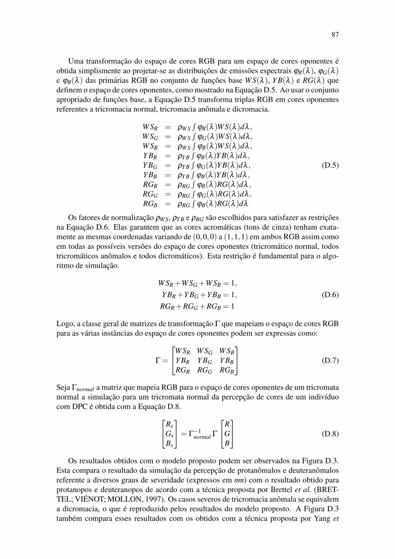
87

Uma transformação do espaço de cores RGB para um espaço de cores oponentes éobtida simplismente ao projetar-se as distribuições de emissões espectrais ϕR(λ ), ϕG(λ )e ϕB(λ ) das primárias RGB no conjunto de funções base WS(λ ), Y B(λ ) e RG(λ ) quedefinem o espaço de cores oponentes, como mostrado na Equação D.5. Ao usar o conjuntoapropriado de funções base, a Equação D.5 transforma triplas RGB em cores oponentesreferentes a tricromacia normal, tricromacia anômala e dicromacia.

WSR = ρWS∫

ϕR(λ )WS(λ )dλ ,WSG = ρWS

∫ϕG(λ )WS(λ )dλ ,

WSB = ρWS∫

ϕB(λ )WS(λ )dλ ,Y BR = ρY B

∫ϕR(λ )Y B(λ )dλ ,

Y BG = ρY B∫

ϕG(λ )Y B(λ )dλ ,Y BB = ρY B

∫ϕB(λ )Y B(λ )dλ ,

RGR = ρRG∫

ϕR(λ )RG(λ )dλ ,RGG = ρRG

∫ϕG(λ )RG(λ )dλ ,

RGB = ρRG∫

ϕB(λ )RG(λ )dλ

(D.5)

Os fatores de normalização ρWS, ρY B e ρRG são escolhidos para satisfazer as restriçõesna Equação D.6. Elas garantem que as cores acromáticas (tons de cinza) tenham exata-mente as mesmas coordenadas variando de (0,0,0) a (1,1,1) em ambos RGB assim comoem todas as possíveis versões do espaço de cores oponentes (tricromático normal, todostricromáticos anômalos e todos dicromáticos). Esta restrição é fundamental para o algo-ritmo de simulação.

WSR +WSG +WSB = 1,Y BR +Y BG +Y BB = 1,RGR +RGG +RGB = 1

(D.6)

Logo, a classe geral de matrizes de transformação Γ que mapeiam o espaço de cores RGBpara as várias instâncias do espaço de cores oponentes podem ser expressas como:

Γ =

WSR WSG WSBY BR Y BG Y BBRGR RGG RGB

(D.7)

Seja Γnormal a matriz que mapeia RGB para o espaço de cores oponentes de um tricromatanormal a simulação para um tricromata normal da percepção de cores de um indivíduocom DPC é obtida com a Equação D.8.Rs

GsBs

= Γ�1normal Γ

RGB

(D.8)

Os resultados obtidos com o modelo proposto podem ser observados na Figura D.3.Esta compara o resultado da simulação da percepção de protanômalos e deuteranômalosreferente a diversos graus de severidade (expressos em nm) com o resultado obtido paraprotanopos e deuteranopos de acordo com a técnica proposta por Brettel et al. (BRET-TEL; VIÉNOT; MOLLON, 1997). Os casos severos de tricromacia anômala se equivalema dicromacia, o que é reproduzido pelos resultados do modelo proposto. A Figura D.3também compara esses resultados com os obtidos com a técnica proposta por Yang et

88

(2 nm) (10 nm) (20 nm) Brettel

P(M

odel

)P

(Yan

g)D

(Mod

el)

D(Y

ang)

Figure D.3: Simulação da visão de protanômalos e deuteranômalos para diversos grausde severidade (expressos em nm). Última coluna: resultado do algoritmo de Brettel etal. tido como referência de precisão para casos de dicromacia.P/D (Model): simulaçõesde Protanomalia/Deuteranomalia com a técnica proposta. P/D (Yang): simulações deProtanomalia/Deuteranomalia com a técnica proposta por Yang et al..

al. (YANG et al., 2008). Note como os resultados do modelo proposto são mais consis-tentes do que os resultados de Yang et al..

O modelo proposto foi validado através de experimentos envolvendo o teste Farnsworth-Munsell 100-Hue (FM100H) (FARNSWORTH, 1957). Foi implementada uma versãocomputadorizada do teste para aplicação em indivíduos tricromatas normais e indivíduoscom DPC. No caso, também se aplicou em tricromatas normais uma versão do teste queusava o modelo proposto para simular a percepção de indivíduos com DPC, simulandoa aplicação do teste nestes indivíduos. Os resultados dos testes simulados foram equiva-lentes aos resultados do teste original aplicado a indivíduos com DPC.

D.2 A Técnica de Realce de Contraste de Cores

A técnica de recoloração proposta se baseia na seguinte observação: sempre que indi-víduos portadores de dicromacia sofrem alguma perda significativa na percepção de con-traste de cor, boa parte deste contraste pode ser recuperado se, ao trabalhar num espaço decores perceptualmente uniforme, as cores originais forem projetadas num plano alinhadocom a direção que maximiza a perda de contraste (no sentido de mínimos quadrados). Ascoordenadas dessas projeções se tornam as coordenadas da nova cor no gamut reduzido(2D) dos dicromatas. A Figura D.5 resume este processo, que consiste dos seguintespassos:

89

1. o vetor vab que representa a direção que maximiza a perda de contraste no plano decromaticidade CIE L�a�b� é estimado e

2. as cores originais são projetadas no plano definido por vab e o eixo de luminosidade(L�). As coordenadas das cores projetadas são então rotacionadas em torno deL� para que se alinhem ao plano aproximado ao gamut dos dicromatas. As coresresultantes são usadas na imagem recolorida.

Visando garantir coerência temporal, o algoritmo verifica e corrige mudanças abruptas nosentido de vab.

O gamut de cores referente a cada classe de dicromacia pode ser representada pordois semi-planos no espaço de cores LMS (BRETTEL; VIÉNOT; MOLLON, 1997) epode ser satisfatoriamente aproximada a um plano (VIÉNOT; BRETTEL; MOLLON,1999). A Figura D.4 mostra esses planos mapeados para o espaço de cores CIE L�a�b�.De acordo com Kuhn et al. (KUHN; OLIVEIRA; FERNANDES, 2008a) os ângulos entretais planos e o plano L�b� são θp =−11.48�, θd =−8.11� e θt = 46.37� para protanopia,deuteranopia e tritanopia, respectivamente. As cores ilustradas na Figura D.4 representamos gamuts de cores presentes em cada classe de dicromacia.

(a) (b) (c)

Figure D.4: Planos que se aproximam aos gamuts de cores referentes às percepçõesdos dicromatas no espaço de cores CIE L�a�b� (KUHN; OLIVEIRA; FERNANDES,2008a). (a) Protanopia (θp = −11.48�). (b) Deuteranopia (θd = −8.11�). (c) Tritanopia(θt = 46.37�).

Calcular a direção que maximiza a perda de contraste local (no sentido de mínimosquadrados) referente à percepção de uma imagem I por um indivíduo portador de dicro-macia pode requerer a avaliação, para cada pixel pi 2 I, da perda de contraste entre pi etodos os pixels p j numa vizinhança Ni em torno de pi. Entretanto, devido à coerência es-pacial, os pixels vizinhos tendem a apresentar valores semelhantes. Logo, a estimativa deperda de contraste local para cada pixel pi contra todos os pixels em Ni tende a resultar emtrabalho reduntante. A técnica proposta evita efetuar este cálculo em toda a vizinhançaNi ao recorrer à abordagem para amostragem por pareamento Gaussiano proposta porGrundland e Dogdson (GRUNDLAND; DODGSON, 2007). Neste caso, a contribuiçãode cada pixel pi para a perda de contraste local é estimada para apenas um vizinho p j.As distâncias horizontais e verticais entre pi e p j são definidas aleatoriamente de acordocom uma distribuição Gaussiana univariada com mediana zero e variância (2/π)σ2, ondeσ2 =

√2min(width,height) (GRUNDLAND; DODGSON, 2007). A função min(a,b)

retorna o menor valor entre a e b, e width e height referem-se às dimensões da imagem.Embora a direção que maximiza a perda de contraste local obtida usando esta estratégiade amostragem difira da calculada quando se usa a vizinhança inteira, devido a coerência

90

espacial essas direções tendem a ser suficientemente próximas umas das outras. Visandoevitar �ickering durante a recoloração de seqüências de videos ou animadas, o algoritmoproposto pré-calcula as coordenadas dos p js e as salva numa textura. Durante toda aseqüência, os mesmos pares (pi, p j) são usados.

As Figuras D.5 (a) e (b) ilustram o processo de cálculo da direção que maximiza aperda de contraste para dois pares de cores, (c1,c2) e (c3,c4), representados como peque-nas esferas no espaço de cores L�a�b�. c01 a c04 ilustram as projeções das cores c1 a c4,respectivamente, no plano do dicromata, e representam suas percepções de cores pelosdicromatas (Figure D.5(a)). Sendo L�a�b� aproximadamente perceptualmente uniforme,a relativa perda de contraste de cor vivenciada pelo dicromata ao observar um par de cores(ci,c j) (referente a um observador com visão de cores normal) pode ser estimado como

l(ci,c j) =kci� c jk�kc0i� c0jk

kci� c jk, (D.9)

onde k.k é o operador de comprimento de vetores. Para este par de cores, a direção deperda de contraste é dada por ϑi j = ci� c j. Para evitar inversão de polaridade (KUHN;OLIVEIRA; FERNANDES, 2008a), o algoritmo proposto preserva a coordenada de lumi-nosidade (i.e., L�) das cores originais. Logo, é suficiente calcular a direção que maximizaa perda de contraste apenas no plano de cromaticidade. Não há vantagens em efetuar estecálculo nas três dimensões do espaço L�a�b�, além disso, seria requerido calcular os au-tovetores numa matrix 3�3 em vez de numa 2�2. Portanto, seja wi = l(ci,c j)ϑi j o vetorque representa a perda de contraste ao longo da direção ϑi j associada ao pixel pi e seja

M =

wa�

1 wb�1

wa�2 wb�

2. . . . . .

wa�n wb�

n

(D.10)

uma matriz cujas linhas contêm as coordenadas dos vetores de cromaticidade referentesà perda de contraste de todos os pixels na imagem I, os elementos da i-ésima linha de Mrepresentam as projeções de wi no plano a�b�, logo, vab pode ser obtido como o autovetorda matriz 2� 2 MT M cujos autovalores correspondentes têm o maio valor absoluto. Afim de resolver a equação característica correspondente, o algoritmo atribui o valor um àcoordenada b� de vab e soluciona para sua coordenada a�.

Quando a percepção de um dicromata sofre com uma significativa perda de contrastede cor, a projeção ortográfica das cores originais no plano definido pelos vetores L� e vabtendem a proporcionar um maior espalhamento das cores se comparado à projeção diretano plano dicromático. Esta situação é ilustrada na Figura D.5 (a) e (c). Ao transferirmosa relação espacial entre as cores projetadas no plano L�-vab para o plano dicromático,uma imagem com melhor contraste de cores é produzida. Para isto, rotaciona-se as coresprojetadas em torno do eixo L� visando o alinhamento destas com o plano dicromático.A Figura D.5 (d) ilustra esta operação, que preserva as cores acromáticas da imagemoriginal.

Coerência temporal é um requisito importante para as técnicas de recoloração de im-agens, já que mudanças sutis na cor de um objeto durante uma sessão interativa de visu-alização ou animação pode incomodar bastante os observadores. Se a direção de vab épraticamente paralela ao eixo a�, uma pequena mudança nas cores de entrada pode im-plicar na inversão do sinal do componente b� de vab (veja Figura D.5(b)). Entretanto, para

91

(a) (b) (c) (d)

Figure D.5: Ilustração dos passos do algoritmo de recoloração proposto. (a) As cores c1a c4 são percebidas por um dicromata como c01 a c04, respectivamente (suas projeções noplano referente ao gamut do dicromata). A relativa perda de contraste, quando um parde cores (ci,c j) é percebido por um dicromata, é dada por l(ci,c j) = (kci− c jk− kc0i−c0jk)/(kci− c jk), o que acontece ao longo da direção ϑi j = ci− c j. (b) A direção vab (emazul) que maximiza a perda de contraste local (no sentido de mínimos quadrados) é calcu-lada como o principal autovetor da matriz MT M, onde M está definido na Equação D.10.(c) A projeção das cores originais no plano definido por vab e L�. (d) As cores finaisobtidas após a rotação das cores projetadas c00k em (c) em torno de L� para que se alinhemcom o plano do dicromata.

a solução da equação característica associada com o cálculo de vab, foi arbitrado o valor1 ao seu componente b�, como uma maneira possivel de evitar a solução trivial vab = 0.Isto restringe o sinal do componente b� de vab como positivo, causando a inversão dosinal do componente a� para adaptar a mudança na direção de vab. Esta inversão podeprovocar mudanças abruptas nas cores dos pixels recoloridos entre quadros consecutivos(e.g., pixels azuis poderiam virar amarelos e vice-versa). Para evitar a ocorrência destesartefatos durante uma sessão interativa de visualização (ou animação) o algoritmo registraas coordenadas do vetor vab referentes ao quadro atual para comparação com as coorde-nadas do vetor obtido no próximo quadro. Caso o ângulo entre ambos os vetores (atual eanterior) se aproxime de 180�, o algoritmo inverte o sentido do vab atual, visando forçarconsistência de cor. Apesar de simples, esta é uma solução eficaz.

Os resultados do algoritmo proposto estão apresentados na Figura D.6 que os comparacom os resultados obtidos pela técnica de Kuhn et al.. A Tabela D.2 resume o ganhode performance alcançado pelo algoritmo proposto ao comparar os tempos de execuçãode ambas as versões (CPU e GPU) com a técnica de Kuhn et al. para um conjunto desete imagens de diversos tamanhos. Os registros na tabla estão apresentados em ordemcrescente pelo número de pixels das imagens. Como pode-se observar, em ambas asversões (CPU e GPU), a técninca proposta apresenta ganhos de performance de até duasordens de magnitude mais rápidas do que a técnica de Kuhn et al. para imagens de até800� 800 pixels. Como o custo do algoritmo proposto é linear no número de pixels, aaceleração alcançada apresentará ganhos em performance ainda mais significativos paraimagens com maiores dimensões.

D.3 Conclusões

Este capítulo apresentou resumidamente as técnicas propostas nesta dissertação demestrado que consistem de um modelo para simulação da percepção de cores e uma téc-nica de realce de contraste de cores.

92

Imagem (tamanho)CPU GPU

Proposta Kuhn Proposta KuhnTempo Tempo Tempo Tempo

Flame (288x184) 0,055 1,148 0,019 0,121Chart (500x300) 0,191 2,707 0,020 0,106Foot (446x446) 0,252 3,743 0,021 0,307Brain (532x523) 0,292 5,053 0,023 0,577Knee (528x528) 0,341 5,217 0,022 0,313Europe (596x486) 0,385 5,361 0,023 0,565Nebula (800x800) 0,614 11,73 0,028 1,145

Table D.2: Comparação entre as performances (em segundos) da técnica proposta e atécnica apresentada por Kuhn et al. (KUHN; OLIVEIRA; FERNANDES, 2008a) parasuas versões CPU e GPU. Devido ao custo linear da técnica proposta, a aceleração relativaé ainda melhor para imagens de maiores dimensões.

Referência Protanopo Recolor. (Proposta) Recolor. (Kuhn)

Cha

rtE

urop

eB

rain

Foot

Figure D.6: Imagens comparando os resultados de recolorações da técnica proposta coma técnica apresentada por Kuhn et al. (KUHN; OLIVEIRA; FERNANDES, 2008a).

93

O modelo proposto é o primeiro a consistentemente tratar visão de cores normal,tricromacia anômala e dicromacia usando um framework unificado. Por meio de exper-imentos controlados com usuários, foi demonstrado que os resultados produzidos pelomodelo proposto se equiparam à percepção de indivíduos com deficiências na percepçãode cores. Os resultados do modelo proposto foram comparados com os obtidos com mod-elos existentes para simulação da percepção de tricromatas anômalos (YANG et al., 2008)e dicromatas (BRETTEL; VIÉNOT; MOLLON, 1997). Tais comparações indicaram queos resultados do modelo são superiores aos de Yang et al. (YANG et al., 2008) para tri-cromacia anômala e equivalentes aos de Brettel et al. (BRETTEL; VIÉNOT; MOLLON,1997) para dicromacia.

A técnica de recoloração apresentada é a primeira a oferecer recoloração de imagenspara dicromatas em tempo-real, com coerência temporal e alta qualidade. Seu custo com-putacional varia linearmente com o número de pixels de entrada e pode ser eficientementeimplementado em GPUs. Foi mostrado que os resultados produzidos com a técnica pro-posta apresentam resultado pelo menos tão bons quanto os obtidos com as técnicas estado-da-arte, sendo que com tempos de execução até duas ordens de magnitude mais rápidos.Além disso, os resultados da técnica proposta permitem o desenvolvimento de aplicaçõesmais amigáveis para indivíduos com deficiência na percepção de cores, já que o baixocusto computacional desta técnica faz dela uma solução adequada para implementaçãoem telefones celulares e outros dispositivos móveis equipados com câmeras. Em tais dis-positivos, a capacidade de recoloração desta técnica pode ser uma ferramenta útil paraauxiliar indivíduos com deficiência na percepção de cores em diversas tarefas cotidianas.

A integração de ambas as técnicas com um sistema de visualização foi bem suce-dida, utilizando uma abordagem minimamente invasiva através de suas implementaçõesvoltadas para GPUs. A Figura D.7 exibe algumas telas deste aplicativo com as opçõespara simular a percepção de indivíduos com DPC (Figura D.7 centro) e recolorir pararealçar contraste de cores para estes indivíduos (Figura D.7 direita).

Figure D.7: Integração das técnicas propostas com um sistema de visualização existente.Esquerda: imagem de referência como percebida por um indivíduo com visão de coresnormal. Centro: simulação da percepção de deuteranopos da imagem de referência us-ando o modelo proposto. Direita: imagem recolorida para deuteranopos usando a técnicaproposta. Implementações minimamente invasivas voltadas para GPUs.

94