Embed Size (px)
Citation preview

A Model for the Parasitic Disease BilharziasisAuthor(s): Trevor LewisSource: Advances in Applied Probability, Vol. 7, No. 4 (Dec., 1975), pp. 673-704Published by: Applied Probability TrustStable URL: http://www.jstor.org/stable/1426396 .
Accessed: 14/06/2014 02:52
Your use of the JSTOR archive indicates your acceptance of the Terms & Conditions of Use, available at .http://www.jstor.org/page/info/about/policies/terms.jsp
.JSTOR is a not-for-profit service that helps scholars, researchers, and students discover, use, and build upon a wide range ofcontent in a trusted digital archive. We use information technology and tools to increase productivity and facilitate new formsof scholarship. For more information about JSTOR, please contact [email protected].
.
Applied Probability Trust is collaborating with JSTOR to digitize, preserve and extend access to Advances inApplied Probability.
http://www.jstor.org
This content downloaded from 185.44.78.115 on Sat, 14 Jun 2014 02:52:45 AMAll use subject to JSTOR Terms and Conditions

Adv. Appl. Prob. 7, 673-704 (1975) Printed in Israel
? Applied Probability Trust 1975
A MODEL FOR THE PARASITIC DISEASE BILHARZIASIS
TREVOR LEWIS, University of Bradford
Abstract
In this paper we develop a model for describing the spread of the parasitic disease bilharziasis. The detailed model first developed (Model A) is made more tractable by replacing infecting population sizes by their expected values in the transition probabilities, giving Model B. Using this approximating model it is
possible to examine the nature of the spread of the disease and the effects of control measures. The effects of a particular control measure are examined in order to compare Models A and B.
BILHARZIASIS; PARASITIC DISEASE; STOCHASTIC MODEL; ENDEMIC DISEASE;
CONTROL MEASURES; SIMULATION
1. Introduction
Bilharziasis, or schistosomiasis as it is sometimes known, is probably the most
important of the helminthic diseases being endemic in many parts of Africa, Asia and South America. The parasites which cause the disease are trematodes of the
genus Schistosoma, three of which, namely S. haematobium, S. mansoni and S.
japonicum are pathogenic to man. These parasites need a definitive host (usually man) and an intermediate host (a fresh-water snail) in order to complete their life cycle.
The adult male and female worms live in the blood vessels of the definitive host where they mate and produce eggs which are excreted from the host in the urine or faeces. If these eggs reach water they develop into larvae, called
miracidia, which can penetrate the skin of fresh-water snails. In the snails the miracidia form cysts and multiply asexually producing enormous numbers of fork-tailed larvae, the cercariae, which escape into the surrounding water. If these cercariae gain contact with the skin of a definitive host, they can penetrate it and pass via the bloodstream to the liver where they develop into adult worms. These worms then mate and migrate to the blood vessels where egg-laying takes
place. And so the life cycle of the parasite is completed. It has been estimated that more than 150 million people are infected with
bilharziasis (W.H.O. (1965)) and that in Egypt alone, the disease costs $560 million annually (Farooq (1967)). Since these estimates were produced the
Received 3 March 1975.
673
This content downloaded from 185.44.78.115 on Sat, 14 Jun 2014 02:52:45 AMAll use subject to JSTOR Terms and Conditions

674 TREVOR LEWIS
situation has not improved. The methods used to control the disease have been more than balanced by the effects of new agricultural developments. These
developments have produced ideal conditions for the transmission of the disease
by creating dense human settlements around the irrigation systems and man- made lakes. Details of the control measures used against the disease, as well as of the life cycle of the parasite, and the effect of the parasite on its hosts, can be found in Jordan and Webbe (1969).
In this paper a model is developed which is suitable for describing the
epidemic (i.e. transient) and endemic (i.e. equilibrium) properties of bilharziasis. In particular, the model can be used for investigating the effect of the various control measures on the endemic level of the disease.
Work on the mathematical theory of epidemics has been reviewed by Bailey (1957) and Dietz (1967, 1972). Most of this work is concerned with developing and extending the classical epidemic models (i.e., the simple, general and carrier-borne epidemics). However, these models are not generally suitable for
describing the spread of a parasitic disease such as bilharziasis for the following reasons.
(i) In the study of an endemic disease, the level at which the disease maintains itself is of interest. This necessitates studying the populations con- cerned over a long period of time and so immigration, birth, death and
emigration must be taken into account. Thus a closed population model is not
appropriate.
(ii) in models for describing the spread of disease it is generally assumed that all infected individuals are equally infectious. In the case of a parasitic disease it is more reasonable to suppose that the infectivity of an individual depends on the number of parasites within the individual, the actual dependence being deter- mined by the life cycle of the parasite within the host.
(iii) When studying the spread of bilharziasis there are three populations which must be explicitly taken into account, namely the humans, the snails and the parasites.
(iv) In order to study the effects of control measures on the endemic level of disease it is necessary to develop a model which is detailed enough to represent the measures adequately.
Because of the necessity for a detailed model, the model developed in this
paper is developed only with bilharziasis in mind. However, the basic approach could be used for any parasitic disease. Macdonald (1965) and Nasell and Hirsch
(1971, 1973) have given models for describing the endemic level of bilharziasis and the effects of control measures on it. The model presented in this paper is more general in nature and more realistic in assumptions.
This content downloaded from 185.44.78.115 on Sat, 14 Jun 2014 02:52:45 AMAll use subject to JSTOR Terms and Conditions

A model for the parasitic disease bilharziasis 675
2. A model for bilharziasis
The stochastic model we now develop to describe the spread of bilharziasis takes into account interactions between the human, snail and parasite popula- tions.
2.1. The human population. We suppose the human population is subject to a linear immigration-death process with rates pi and 8, respectively. We assume that the size of the human population is fairly constant, in which case we. may group together births and immigrations to give the overall immigration rate p,. Similarly 81 is the overall death rate taking into account both deaths and
emigrations. Let H (t) be the size of the human population at time t. Then if H (t) = h, the
possible transitions involving a change in the human population size in a short interval of time (t, t + 8t) are:
(i) a human immigration,
T1 h -- h + 1 with probability pi 8t + o (8t)
(ii) a human death,
T2 h -* h - 1 with probability 81 h8t + o (8t).
We assume that all immigrants are completely free from infection when they enter the population.
2.2. The parasite population within the human population. When the cer- cariae penetrate the human skin they pass via the bloodstream to the liver where
they mature into adult worms. This occurs after approximately thirty days. In the liver the worms mature and most of them mate and migrate to the mesenteric veins or the veins of the vesical plexus, depending upon the species, where
egg-laying begins. In the model we suppose that the rate of cercarial penetration of a human is
proportional to the number of infected snails. This is reasonable since a multiple infection of a snail does not increase its infectivity. Also the lifetime of the cercariae is short (about forty-eight hours) and so the number of cercariae alive at any given time will be proportional to the infected snail population size at that time.
We neglect the time taken for the sucessful cercaria to develop into a mature worm and also assume that mature worms in the liver immediately pair off. The
pair then pass together to the veins where they remain until death. Thus there are never both free female and male worms in the liver together. We assume that the worms do not leave the liver until they have mated. This is reasonable, since there is evidence to suggest that the development of maturity of the worms is hindered by the absence of worms of the opposite sex.
This content downloaded from 185.44.78.115 on Sat, 14 Jun 2014 02:52:45 AMAll use subject to JSTOR Terms and Conditions

676 TREVOR LEWIS
The death rate of the paired male is very small compared with that of the female. The reason for the difference is that the female runs the risk of damage each time she lays eggs (approximately twelve times a day). So the death rate of the pair is approximately that of the female. We assume that the remaining member of the pair plays no further role in producing eggs.
For individual j (j = 1, 2, - - - , H (t)) alive at time t, let
Fj (t) = the number of free female worms in the liver,
Mj (t)= the number of free male worms in the liver, and
QO (t)= the number of worm pairs within the individual.
Also let S (t) be the number of infected snails at time t. Then with above
assumptions, if F, (t) = f,, Mj (t) = mj and Q, (t) = qj for each j, and also H (t) = h and S (t) = s, we have the following possible transitions involving a
change in the parasite population within individual j (j = 1, 2, ... , h) in a short interval of time (t, t + 8t);
(i) a penetration by a female parasite,
(a) if m = 0 fj -- fj + 1 T3 with probability ! v1 s8t + o (8t)
(b) if mj>O (m, m) - (m 1,q, +1)
(ii) a penetration by a male parasite,
(a) if f-
= 0 m,-> m +1 T4 with probability ? v1 s8t + o (8t)
(b) if f, >0 (f,q,)-(f-1- 1, qj + 1)
(iii) a death of a worm pair,
T5 q, -- qj - 1 with probability A1 qj 8t + o (8t)
where vi is the penetration rate of cercariae per human per infected snail and As is the death rate of worm pairs.
2.3. The snail intermediate host population. A detailed account of the effect of the parasite on the snail intermediate host is given by Jordan and Webbe (1969).
In our model we make the very reasonable assumption that once a snail becomes infected, it remains infected until death. The rate of infection per susceptible snail is taken to be (y + v2 q), where y is the rate of infection of snails due to reservoir hosts (i.e., other definitive hosts, for example rats, cows and dogs), v2 is the rate of infection per worm pair within the human population, and q is the number of worm pairs within the human population (i.e., q =
IX=, q;). y
can be taken as zero in the case of S. haematobium, small in the case of S.
This content downloaded from 185.44.78.115 on Sat, 14 Jun 2014 02:52:45 AMAll use subject to JSTOR Terms and Conditions

A model for the parasitic disease bilharziasis 677
mansoni, but it can be large in the case of S. japonicum since the reservoir hosts can account for more than half of the miracidia released into the snail habitat
(Hairston (1962)). The assumption that y is constant implies that the infectivity of the reservoir host population remains approximately constant, being un- affected by changes in the infectivity of the human population. This is reasonable since generally the domestic animals are poor hosts, and the natural habitat of the wild animal reservoir hosts is usually away from the human source of infection. As far as the rate of infection due to the human population is concerned, this is taken to be proportional to the number of paired worms within the human population. This is reasonable since the number of miracidia alive at a given time is proportional to the egg-output of the worms at that time since the lifetime of a miracidium is short (approximately twenty-four hours). The
egg-output is in turn proportional to the number of paired worms within the human population.
The infection of snails results in an increase in their death rate. So if 82 and 82
are respectively the death rates for susceptible and infected snails, 82< 82. Infection also results in increased sterility and a decrease in the hatchability of the eggs that are produced. It follows that the birth rate of snails from
susceptible snails (32) is greater than that from infected snails (32). This leads to the inequality,
(2.1) 82 - < 2 <82- 2.
Now let R (t) be the number of susceptible snails at time t. Then if R (t)= r, S (t)= s, H (t)= h and Q (t) = I=, O, (t)= Ih, q, = q the following are the
possible transitions involving changes in the snail population sizes in a short interval of time (t, t + 8t);
(i) a susceptible snail immigration,
T6 r -- r + 1 with probability p2 8t + o (8t)
(ii) a susceptible snail birth,
T7 r -+ r + 1 with probability (32 r + 02 S) 8t + o (8t)
(iii) a susceptible snail death,
T8 r -- r - 1 with probability 82 r8t + o (8t)
(iv) an infected snail death,
T9 s --s - 1 with probability 82sS8t + o (8t)
(v) a snail infection,
T10 (r,s)--
(r- 1, s + 1) with probability (y + v2 q) rSt + o (St).
This content downloaded from 185.44.78.115 on Sat, 14 Jun 2014 02:52:45 AMAll use subject to JSTOR Terms and Conditions

678 TREVOR LEWIS
2.4. Models A and B. We call the model defined by transitions T1 to T10 Model A. Because of our attempt to develop a realistic model, this model is very intractable. However, with a slight modification to transitions T3, T4 and T10 we obtain a much more tractable model.
One of the main problems encountered in stochastic models which describe the spread of disease results from the rate of infection being proportional to the
product of the sizes of the susceptible population and infecting population. We
by-pass this problem by replacing the infecting population size in the rate of infection by its expected value. This technique, which was used by Nasell and
Hirsch, gives a more tractable stochastic model. In our case it causes the interaction between the paired worm and snail populations to be deterministic rather than stochastic. We call the model which uses the expected infecting population sizes Model B and suggest that this model will give a good approximation to Model A, particularly when the population sizes concerned are
large. Let E {(t)} = w (t) and E {S (t)} = y (t), then for Model B we have transi-
tions T1 to T10 with T3, T4 and T10 replaced by the following;
(i) a penetration by a female parasite,
(a) if m, = 0 fi - f; + 1 T'3 with probability vj y (t) St + o (8t)
(b) if m, >0 (m,,q,) -(m -1, qj + 1)
(ii) a penetration by a male parasite,
(a) if f, = 0 m m, + 1
T'4 with probability 2 v, y (t) St + o (8t) (b) if f>O 0
(f,-q),-(f,-1, q+l)
(iii) a snail infection,
T'10 (r, s)-> (r - 1, s + 1) with probability (y + v2 w (t)) rat + o (St).
We proceed to develop Model B and examine how it approximates Model A in Section 8.
3. The distribution of the number of worm pairs within the human population (as predicted by Model B)
Initially we restrict our attention to a single human whose state of infection is known at some time 7. For this individual (individual j) we calculate the distribution of the number of worm pairs at any future time t, given that the individual is still alive and in the community. Transitions T'3, T'4 and T5 lead to a non-homogeneous immigration-death process for the population of worm pairs within the individual.
This content downloaded from 185.44.78.115 on Sat, 14 Jun 2014 02:52:45 AMAll use subject to JSTOR Terms and Conditions

A model for the parasitic disease bilharziasis 679
3.1. The calculation of the immigration rate of worm pairs for individual j. Let N (t) be the number of cercarial penetrations of individual j in (7, t) and define
p. (7, t) = pr (N (t) = n). Then given that N (t) = n, from transitions T'3 and T'4, the only possible transition affecting N (t) in a short interval of time (t, t + St) is a cercarial penetration,
n -* n + 1 with probability vi y (t) St + o (St).
This immediately leads to the forward equations,
d= v y (t)(pn- - pn) n = 0, 1, -
where p-,(7, t)= 0 and p, (7, 7) = no(n,O is the Kronecker delta). And so the
generating function G (z, T, t) = n=o p, (r, t) z " satisfies the equation,
aG
- vi y (t)(z - 1) G
with the initial condition G (z, r, 7) = 1. This is solved to give
G (z, 7, t) = exp {(z - 1)a (7, t)} where r2
a(t, t2) = y (u) du.
Thus
(3.1) p (, t) e (T n=0,1,-
Now suppose that F, (7) = k (k = 0, 1, - - -) and M, (7) = 0. Define F (7, t) and M (7, t) to be respectively the number of penetrations of individual j by female and male cercariae in (7, t). Then for t > 7,
pr {number of pairs is increased by 1 in
(t, t + 8t) Fj (7) = k, M,(7) = 0}
= pr{penetration by a female cercaria in
(t, t + St)} pr{F (, t)+ k < M (r, t)}
+ pr {penetration by a male cercaria in
(t, t + St)} pr {F (7, t)+ k > M (r, t)}
+ o (St) = v1 y (t) 8t (pr {F (r7, t) + k < M (r7, t)}
+ pr {F (7, t)+ k > M (7, t)}) + o (8t)
(3.2) = v-i y (t) (1 - pr {F (7, t) + k = M (r, t)}) Bt + o (St).
This content downloaded from 185.44.78.115 on Sat, 14 Jun 2014 02:52:45 AMAll use subject to JSTOR Terms and Conditions

680 TREVOR LEWIS
By a simple combinatorial argument,
pr {F (, t)+k = M (7, t)}
= pr{F(r, t)+ k = M (r, t)( n penetrations in (7, t)}p, (7, t) n=k
S 1) k))
pn (7, ti) n=k k 2 I(n + k)
where (n = 0 if n, and n2 are not both integers.
Putting 21 = n - k and substituting for pn (7, t) from (3.1) we have
pr {F (7, t) + k = M (7, t)}
S(1)21+k!(21+ k){v•(r',t
)21+k e-(t) -
o I 2 l+ k (21 + k)! e
= Ik (v1 a (7, t)) e- 'va('
where
Ik(X) (x /2)21+k I ) I
ot! (1 + k)!
is the modified Bessel function of order k. Substituting in (3.2) we have,
pr{number of pairs is increased by 1 in
(t, t + 8t) Fj (7) = k, Mj (r) = 0}
= 2 v1 y (t){1 - Ik (v1 a (r, t)) e•v'a"I } t + o (t).
Similarly for F, (7)= 0 and Mj (7)= k (k = 0, 1, - ). Hence if we define
K, (7)= max (F, (7), M, (7)),
pr{number of pairs is increased by 1 in
(3.3) (t,t + 8t)IKj(7)= k}
= V1 zk (7, t) St + o (5t)
where
zk(7-, t) = 2y(t){1 - Ik (v •a(, t))e-va(It)}.
3.2. The distribution of the number of worm pairs within individual j. We are
now in a position to investigate the distribution of the number of worm pairs within individual j at time t (t > 7), given that the individual is still alive and in the community at time t. Define p, (7, t) =
pr{Q, (t) = m JQ, (7) = c, K; (7) = k}. Then given that Q1 (t) = m and using
This content downloaded from 185.44.78.115 on Sat, 14 Jun 2014 02:52:45 AMAll use subject to JSTOR Terms and Conditions
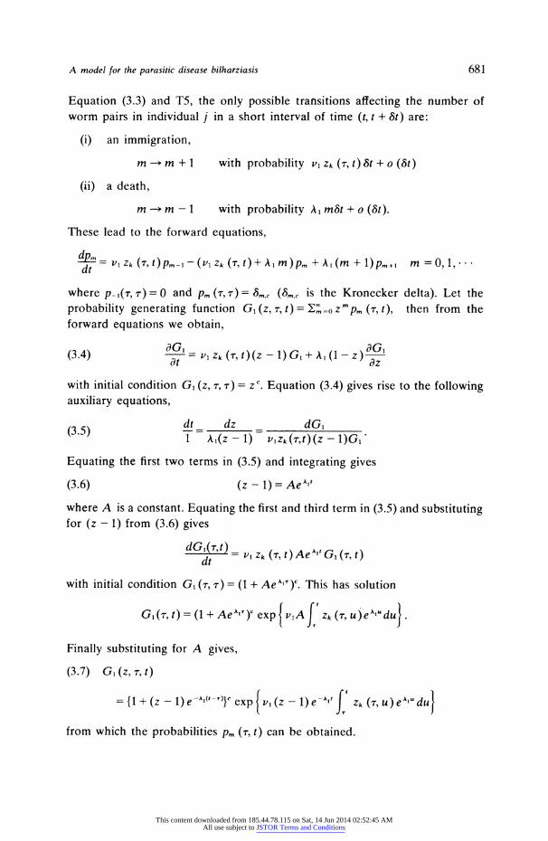
A model for the parasitic disease bilharziasis 681
Equation (3.3) and T5, the only possible transitions affecting the number of worm pairs in individual j in a short interval of time (t, t + St) are:
(i) an immigration,
m - m + 1 with probability vI zk (r, t)St + o (St)
(ii) a death,
m -- m - 1 with probability A m&t + o (6t).
These lead to the forward equations,
dt
where p_,(r,
7)= 0 and pm (T,7)= 6m,, (8m,c is the Kronecker delta). Let the
probability generating function G, (z, 7, t) = '=o z "Pm (7, t), then from the forward equations we obtain,
(3.4)
G, G
(3.4) -1t
- 4 (7r, t)(z - 1)G, + A (1 - z) dt dz
with initial condition G, (z, r, 7) = Zc. Equation (3.4) gives rise to the following auxiliary equations,
dt dz dG1 (3.5) 1 Al(z - 1) V-lZk(T,t)(Z
- 1)G,
Equating the first two terms in (3.5) and integrating gives
(3.6) (z - 1)= AeA'
where A is a constant. Equating the first and third term in (3.5) and substituting for (z - 1) from (3.6) gives
dG( Vi Zk (r, t) Ae^"' G, (r, t) dt
with initial condition G1 (7, 7) = (1 + AeA"")c. This has solution
G,1(, t)= (1+ AeAT")c exp vA zk (7, u)eu'"du .
Finally substituting for A gives,
(3.7) G, (z, 7, t)
={1+(z - 1)e-*,"-)}c
exp VI(z -1)e- zk (r, u)e*,"du
from which the probabilities pm (7, t) can be obtained.
This content downloaded from 185.44.78.115 on Sat, 14 Jun 2014 02:52:45 AMAll use subject to JSTOR Terms and Conditions

682 TREVOR LEWIS
From Equation (3.7) we see immediately that Qj(t) is the sum of two independent random variables, one binomial with parameters c and e-Ait,-') and the other Poisson with mean v1 e- 1' f' k (r, u) e Au du. In particular from (3.7) we obtain the expected number of pairs within individual j at time t (t > 7), given that Qj (r7)= c and Kj (7)= k.
(3.8) E {Qj (t) Q, (r) = c, Kj () = k} = d1Z-=
ce-All + VI k (r,
where
(3.9) fk (r, t) = e-Arf Zk (r, u)e""du.
3.3 The distribution of the number of worm pairs within the entire human
population. We first calculate the expected number of worm pairs within the human population at time t and then give a more general approach in terms of
moment-generating functions. Although this second approach can be used to obtain the expected paired worm population size, it is thought that the approach used is more revealing.
3.3.1. The expected number of worm pairs within the human host population at time t. Suppose that at time t = 0 the human population is of size ho and that for individual i (i = 1, 2, ... , ho) QO, (0) = ci and K, (0) = ki. Using Equation (3.8) and T2 we can immediately write down the expected number of worm pairs, within the original human population, at time t.
ho
wl(t) = E {Q, (t)l Qi (0) = ci, Ki (0) = k,} pr(individual
i is still in the population at time t)
(3.10) = e-' i (cie-' + v k, t))
(3.11) = woe -'(As)' + vie -8t nPkfk (0, t),
i=0
where wo = I c, is the total number of worm pairs at t = 0 and nk is the number of the original population with k free worms at t = 0.
Suppose that in (0, t) there are N newcomers into the population and that the
immigrations occur at Ti, 72,'. *, 7N, where each of the 7T satisfy 0 < , < t. If the order is neglected each of the ri is independently uniformly distributed over
(0, t). Since we assume that the immigrants are completely susceptible, for an individual entering the population at time 7, the expected number of pairs at time t > - is
vl e-61(,- ) [o(7, t).
This content downloaded from 185.44.78.115 on Sat, 14 Jun 2014 02:52:45 AMAll use subject to JSTOR Terms and Conditions

A model for the parasitic disease bilharziasis 683
Thus since the r, are independently uniformly distributed over (0, t), the
expected number of pairs from the N immigrants is
w2(tIN)= PN
e-8,( 3go(r, t) dr.
Now from T1, N has a Poisson distribution with mean p, t and so the expected number of pairs of worms from the immigrants is
(3.12) w2(t) = v1 p? i e -81(t-') o (7, t) dr.
Thus the expected number of worm pairs in the entire human population at time t is
(3.13) w (t) = w1 (t)+ w2(t).
Note that (3.13) is an expression for w (t) in terms of y (u) for 0 5 u - t. The assumption that immigrants are completely free from infection is reasona-
ble since many of the immigrations are in fact births. However, an influx of many infected people into a region where the disease is not present, as sometimes
happeris in new agricultural developments, can be studied by using the initial conditions.
3.3.2. The moment-generating function of the number of worm pairs in the entire human population. Suppose that there are N immigrations of susceptible humans in (0, t) at times
7•, 72,''5 , N. Then
O (t)= U1(t)+ U2(t)+ + U(t)+ V1(t).+ V2.(t) . + VN (t) where U, (t) is the number of worm pairs at time t in the ith member of the
original human population (for whom U, (0) = c, and K, (0) = ki) and Vj (t) is the number of worm pairs at time t in the immigrant who joined the population at time
7• (for whom Vi (71) = K, (71) = 0). The U, and Vi are mutually indepen-
dent. Now the moment-generating function of Q (t),
Mo (0, t)=E exp{OQ (t)}
= ENE,T NE,v,,NexpI 0( U, (t)+ V j=1
Using the independence of the variables we have,
(3.14) Mo(0,t)= Eexp 0 U,.(t) ENE,EINEvIT exp O V, (t) = .=1
= M1(O, t)M2(8, t), say.
First consider M1 (0, t). For each i (i = 1,2,. ? . , h0)
This content downloaded from 185.44.78.115 on Sat, 14 Jun 2014 02:52:45 AMAll use subject to JSTOR Terms and Conditions

684 TREVOR LEWIS
E exp{OU, (t)}
= pr (individual is still in the population) GI (e ,O, t)
+pr (individual has left the population by time t)
Se-"8' Gi (e ', 0, t) + (1 - e -,,) where G1 = G1 with c = c, and k = ki. Thus
ho
(3.15) M1 (0, t) = I- {e- 'G' (e ', O, t) + (1 - e -"')}. i=l
Now consider M2 (0, t). Using a similar argument to the above it is clear that,
Evi,,N exp{0Vj (t)} = e-6,'-) G(e0, rj, t) +(1 - e-',-)
where Go = G, with c = k = 0. Thus using (3.7) and (3.9),
Ev l,,exp{0
Vj(t)} = e -'1"-' [exp{v, (et - 1) 3o (ir, t)} - 1] + 1.
Thus
EvNexp 0 V (t) = ETINEVITNexp 0E Vi;(t) j=1 j=1
=N1 e' e-"'-' T)[exp{v~(e - 1) o(r, t)} - 1]+1 dr.
And so,
M2(,t (P) 1e-PtEv, Nexp 9E V; (t) N=O N! j=1
(3.16)
= exp pif e-"~'->'[expf{v,(e -
1)3o(r, t)} - 1]dr
.
So using (3.14), (3.15) and (3.16) we can obtain the moments of the distribution of the number of worm pairs at time t, in terms of the expected number of infected snails. The moment-generating function for the equilibrium distribution is obtained by letting t -*o. As we would expect lim,,.M1 (0, t) = 1 and so Mo (0, c) =
lim,,_. M2 (0t)
4. The distribution of the number of free worms at time t (t > r) in an immigrant entering the community at time r
In order to have complete knowledge of the state of infection of an individual at time t, as well as information about the number of worm pairs, we need to know about the number of free worms. Consider an immigrant entering the community at time r.
This content downloaded from 185.44.78.115 on Sat, 14 Jun 2014 02:52:45 AMAll use subject to JSTOR Terms and Conditions

A model for the parasitic disease bilharziasis 685
pr{the immigrant has k free female worms at time t} =pr{k more females than males penetrate the immigrant in (7, t)}
S 21 + k)
21+k
pr {21+ k penetrations in (r, t)}
= Ik (v) e-v (using Equation (3.1))
where Ik is a modified Bessel function of order k and v = v, a (r, t). Thus
(4.1) pr{ithmigrant has k free worms at time t} = (2- 80,k) Ik (v) e-
where 80,k is the Kronecker delta. Now Ik (v)> Ik2 (v) for integers k, and k2
satisfying 0_-
k, < k2 (Cochran (1967)). Thus the distribution of the number of free worms, given by (4.1), is J-shaped if Io(v) ? 21, (v), otherwise it has a mode at k = 1. Using standard results relating modified Bessel functions (see, for
example, Abramowitz and Stegun (1965)) we obtain the first two moments about zero of the distribution to be ve-v {Io (v) + I, (v)} and v respectively.
4.1. The proportion of people with k free worms (k = 0, 1, - - - ) in the equilibrium situation. We first of all state the following standard result for the integral transform of a modified Bessel function (see, for example, Erd6lyi (1954)). If a> qJ ,
(4.2) e "' Ik (qt) dt = q k d-1D -k
where d = (a2 - q2)1/2 and D = a + d. Now in the equilibrium situation the age distribution of the human population
will be negative exponential with parameter 86. For an individual of age t in a
steady endemic area, from Equation (4.1) we have,
pr(an individual has k free worms lhis age is t) = (2- 80,k) 1k (v1 y (oo) t) e
iY&). Therefore removing the conditioning on t,
pr (an individual has k free worms)
= (2- Sno,k)1 e-8"'Ik (vy ()t)e -"y()'dt.
Using Equation (4.2), and after some manipulation, this reduces to
pr(an individual has k free worms)
- (2-
8o,k)po 1 P k=0,1,..
\r lUKY 1+ Po
This content downloaded from 185.44.78.115 on Sat, 14 Jun 2014 02:52:45 AMAll use subject to JSTOR Terms and Conditions

686 TREVOR LEWIS
where
PO== +(2vy1 -1+ y
This is a geometric distribution with a modified first term. Clearly the probability of an individual having k free worms is equal to the expected proportion of the
population with k free worms, when the disease is in the steady endemic state.
5. The distribution of the numbers of susceptible and infected snail intermediate hosts
The transitions which affect the susceptible and infected snail population sizes are T6, T7, T8, T9 and T'10.
Define p,s (t) = pr (R (t) = r and S (t) = s), then the above transitions lead to the following forward equations
dt {P + P2 (r - 1)+ ?2 S}Pr-s + (Y + V2 W (t))(r + 1)pr+l,s-I
+ 82 (r + 1)prs
+ 82 (S + 1) Pr,.si
- {P2 2 r + 32 S + (y + V2 w (t))r + V2 r + 62 S} Pr,s
where r, s = 0, 1, .. and p,, = 0 if r or s is negative. Defining G2 (zi, z2, t)
r=o l=zo SZZ p,.s
and using the above forward equations we obtain the partial differential equation
= p2 (z1 - 1) G2 + {((2 - z1)(y + •2
W (t))+ 2 (1 - z)+ 2z (Z - 1) dt dz1
dz2
Equation (5.1) is difficult to solve, but with a slight simplification the solution is much easier. As we have already stated, the birth rate of snails from infected snails is small compared with that from susceptible snails. Indeed in some situations it can be neglected (i.e., take /32 = 0). Also, if the susceptible snail
population remains approximately constant in size, the birth rate of snails from
susceptible snails can be grouped with the immigration rate to give an overall
immigration rate. Thus /32 = 0 and p2 now becomes the overall immigration rate. So Equation (5.1) simplifies to
OG2 (5.2) G2
p 2(zo1-1) G2 + {(z2- z1)(y + V2 W ())+(1- z1)}2i -? (1- z2)t2
In order to solve (5.2) consider the auxiliary equations
This content downloaded from 185.44.78.115 on Sat, 14 Jun 2014 02:52:45 AMAll use subject to JSTOR Terms and Conditions
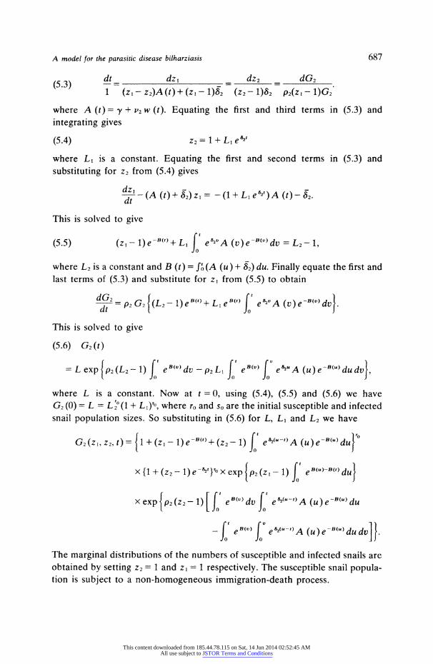
A model for the parasitic disease bilharziasis 687
dt dz1 dz2 dG2 (5.3) 1 (z, - z2)A (t)+ (z,
- 1)82 (z2- 1)82 2(1 - 1)G2
where A (t) = y + v2 w (t). Equating the first and third terms in (5.3) and
integrating gives
(5.4) z2 = 1 + L1 e s
where LI is a constant. Equating the first and second terms in (5.3) and
substituting for z2 from (5.4) gives
dz,(A (t)+ 62) 1= -(1 + L, es')A (t)- 92. dt
This is solved to give
(5.5) (z,- 1) eB)+ L, e4"A (v)e(0)'dv =L2- 1,
where L2 is a constant and B (t) = f'o(A (u) + 82) du. Finally equate the first and last terms of (5.3) and substitute for z1 from (5.5) to obtain
dt = P2 G2 (L2- 1) eB')+ L1 eB(t) f
e6"A (v)e-B(,)dv .
This is solved to give
(5.6) G2(t)
= L exp p2(L2- 1) eB(v) dv - p2L,
L ' e"(v) A (u)eB') dudv ,
where L is a constant. Now at t =0, using (5.4), (5.5) and (5.6) we have
G2(0)= L = L2(1 + L )so, where ro and so are the initial susceptible and infected snail population sizes. So substituting in (5.6) for L, L, and L2 we have
G2(z, z2,
t)= 1 +(z1 -
1)eB(t)+(z2- 1) f e"-)A (u)e-B(e)du}
x {1 + (z2- 1) e-t'}~ x exp p2(z- 1) feB(u)-B(t) du
x exp p2(Z2- 1) [ eB'() dvf e "-)A (u)e-"'du
-' eB(v) o e(u-t)A (u)e-B() dudv]J.
The marginal distributions of the numbers of susceptible and infected snails are obtained by setting z2 = 1 and z, = 1 respectively. The susceptible snail popula- tion is subject to a non-homogeneous immigration-death process.
This content downloaded from 185.44.78.115 on Sat, 14 Jun 2014 02:52:45 AMAll use subject to JSTOR Terms and Conditions

688 TREVOR LEWIS
6. Differential equations for the expected population sizes
Rewriting Equation (3.13) and substituting for w, (t) and w2 (t) from Equa- tions (3.11) and (3.12) we have
(6.1) w (t)
= woe -A'+)+ vi e - nk
k (0, t) + v1 pi e-'81() ,o(7, t) d. k=0 0
Differentiating the defining equation (3.9) we have
d
dt jk (rt)= -A1 k ( rt)+ zk ( rt).
And so differentiating (6.1) gives
dw (6.2) dt = -(A1 + 81)w + 4 (y (v), O v t; t),
where
b(y(v), O-v-t;t)=v e t
nkzk(O,t) + vi pl e-' '"zor(7,t)dr. k=0 0
The equations for the expected numbers of susceptible and infected snails are obtained from Equation (5.1). Differentiating with respect to z, and then setting
zi = z2 = 1 we have
dx - - (6.3) P2 - 1(52 - 02)+ + V2 w)}x +02 y,
where x (t) = E {R (t)}. Differentiating (5.1) with respect to z2 and then setting Z1 = z2 = 1 gives,
(6.4) (y + v2 w)x - 82 y. dt
It can be shown that Equations (6.2), (6.3) and (6.4) have a unique solution, which remains bounded if and only if 82 - 2 > 0 (note Inequality (2.1)). The only exception to this is when the disease is initially absent and 52- 32 _
0 and y = 0. In this case w (t) = y (t) = 0 for all t and x (t) increases without bound. This
highlights the fact that when 82- 32 > 0 and #2 -32 - 0, it is the presence of the
parasite which limits the growth of the snail population. For the case 82- 32 < 0, it is worth remarking that environmental restrictions
will eventually limit the growth of the populations. For example, overcrowding may well reduce the birth rate of the snails and increase their death rate. We will not deal with this situation as we restrict our approach to constant parameter values.
This content downloaded from 185.44.78.115 on Sat, 14 Jun 2014 02:52:45 AMAll use subject to JSTOR Terms and Conditions
A model for the parasitic disease bilharziasis 689
Since we are interested in the attainment of endemic levels we restrict our attention, from now on, to the case 82- 32 > 0, but exclude the above special case.
7. An investigation of the equilibrium means for Model B
We now consider the endemic properties of the disease and examine the
equilibrium values of the expected population sizes.
7.1. Equations relating the equilibrium means. The equilibrium values of the
expected numbers of worm pairs, susceptible snails and infected snails are obtained from Equations (6.2), (6.3) and (6.4) by setting dw/dt = dx/dt = dyldt = 0 and letting t x, giving the following equations:
(7.1) (A, + 6,) w (oc)= uv, plimr e "'-)zo(,r,t)dr
(7.2) P2 + Y (2 ) = - 2 2+ 3 + V2 W (O)}X (O0)
(7.3) 6 y (o)= {y + v2 w (OC)}x (O).
Consider Equation (7.1), in particular lim,_.f'o
e '-7) zo (7, t) dr. Putting v = t - r gives
(7.4) L (t)= e-8'"-' zo (7, t) dr = e-,zo(t
- v, t)dv.
We prove the following lemma.
Lemma.
lim L (t)= {1-Io(u) e "}exp( )du.
Proof. Choose e > 0. Then for a large enough t (which we suppose is fixed for the moment) we can find vo < t such that for all t' satisfying vo < t' < t,
(7.5) 1 Y (t')- y () < E.
Splitting the integral in (7.4) we have
L (t) = L, (t)+ L2 (t),
where
and
L2(t)= e -Zo (t-v,t) dv.
This content downloaded from 185.44.78.115 on Sat, 14 Jun 2014 02:52:45 AMAll use subject to JSTOR Terms and Conditions

690 TREVOR LEWIS
Consider L, (t). Since 0 5 Ik (u) e-" 1 for all u - 0 and k = 0, 1,
(7.6) L, (t) f: , e-A1V 2dv = ()e 8,o - 1} e-','
-*0 as t - oo.
Consider L2(t). Using (7.5), we have that since {1- lo(u)e-"} is an increasing function of u for u ? 0,
(7.7) N(- E, t) L2 (t) N (E, t)
where
N(e, t)= 2 o
e-81v {1 - Io(vi (y (o) + e) v) e-"1(Y(=)+e.} dv.
Letting t -* , Inequalities (7.7) hold for all e > 0, and so we have
(7.8) lim L2(t) = f e 8 {1 - Io(vi y (o) v) e-"'Y(')} dv.
Setting u = vi y (o) v in (7.8) and noting (7.6) completes the proof.
Consider the standard result given in Equation (4.2). Taking k = 0; a = 1+ b and q = 1 we have that for b > 0,
e-bu 1- Io (u) e-} du = b-1 1- 1+ 2
Using the above lemma and this result we obtain from Equation (7.1) the
following relationship between w (ro) and y (oc):
21(A + 8+) j1) ( +
(7.9) i.e., w (x) = 2 y (x)f{1 - (1 + 2a1 y (0))-1/2
defining al = V and
O1- 81 1, + 51
We note that although L (t) (defined in (7.4)) is a function of y (v) for 0 ? v ? t, L (o) depends only on y(oo). This is a desirable property which we would expect, since it implies that the value of w (oo) does not depend on the path taken by y (t), only on the limiting value y (oo}.
Consider now the other two equations relating the equilibrium means, Equations (7.2) and (7.3). Subtracting Equation (7.3) from (7.2) we have,
(7.10) (82- 32)X (oC)+ ($2-/32)y (C) = P2.
Using Equation (7.10) we can eliminate x (oc) from (7.3) to give
This content downloaded from 185.44.78.115 on Sat, 14 Jun 2014 02:52:45 AMAll use subject to JSTOR Terms and Conditions

A model for the parasitic disease bilharziasis 691
(7.11) w () =
Y((0-
) Y a2(1 - K)(U2 - y ( 2)) V2
where
2P2 a2- 622
and K2= . 82-92 82- P2 22 7.2. Examination of the solutions to Equations (7.2), (7.3) and (7.9). A value
for y (oo) uniquely determines w (0o) and x (0o) using Equations (7.10) and (7.11), so we consider only y (0o). Combining Equations (7.9) and (7.11) we obtain the
following equation for y (oo),
(7.12) a,'", y(OO){ - 2(1 + 2ay(M)) y(oo) Y 2
ya2(1 - K)(02 - y(oo)) V2
This equation is satisfied by y (oo)= 0 provided y = 0, and the corresponding values for w (oo) and x (oo) are 0 and p2/(82- 12) respectively. So the disease can die out if and only if y = 0 and 82 >32. In order to examine non-zero solutions to (7.12), reduce it to the form
(7.13) f (u) = g (u)
where
f(u)= (1+ au)-112 and g(u)= 1- a2(1- u)
aza3u where
u = ,
a = 2a, (o2, a2aa2 02 2 and
a3 2(2 -2)
y(82 - 32)
Results concerning the roots of (7.13) and the zero solutions of (7.12) are given in Table 1. The properties of the roots of (7.13) can be obtained by simply sketching the curves of f (u) and g (u), and by also noting that f2(u)= g2(ui) is a quintic equation with at most 3 real roots in common with the roots of Equation (7.13). For each of the values of u obtained, there corresponds a triple (w (oo),x (oo), y (on)), which is a set of equilibrium values for the expected population sizes.
7.3. Three sets of equilibrium values. We consider only the case y >0; the case y = 0 follows in a similar way. When 1 < a3 < oc there is a possibility that there are three sets of equilibrium values for the expected population sizes.
This content downloaded from 185.44.78.115 on Sat, 14 Jun 2014 02:52:45 AMAll use subject to JSTOR Terms and Conditions

692 TREVOR LEWIS
TABLE 1
The values of u = y
for different parameter values Cr2
y>0
number of bounds on values of as values of u values of u
1 < a3s<C 1 or 3 Uo< < u<u 0
= a3-- 1 1 Uo< < u<u
- 1 < a3<0 1 u < u < Uo --a< a5 - 1 1 ul< u <a
y=0
number of bounds on values of a2 values of u values of u
1 < a2 < 1 or 3 u = 0, O < u < u,
0<a2-l 1 u=0 - c< a2<0 1 ul< u <ca
Note: uo and u, are defined by g (uo) = 1 and g (u,)= 0
Clearly the set of equilibrium values the Equations (6.2), (6.3) and (6.4) converge to is determined by the initial conditions Wo, ro, So and {nk} (k = 0, 1, - - -). However, the following argument shows that the set of equili- brium values corresponding to the middle value of u gives rise to a spurious equilibrium which cannot be attained in practice.
Let F (u, a,, a2, a3) = f (u)- g (u) = 0.
Then dF aF au aF aa3
-+ = 0. dy au ay aa3 ay
Therefore
aF da3 au _ a3 ay ay D(u) '
where
aF D (u) Huc
Hence
This content downloaded from 185.44.78.115 on Sat, 14 Jun 2014 02:52:45 AMAll use subject to JSTOR Terms and Conditions

A model for the parasitic disease bilharziasis 693
(7.14) =y(oo) "2 =au0? (7.14y y a2a3yuD(u)
Now D (u) is negative for the middle root of (7.13) but positive for the other two. Clearly if the rate of infection of snails due to reservoir hosts is increased we would expect y (oo) to be increased. But this is not the case for the middle root, since from Equation (7.14) ay (oo)/ay takes the sign of D (u).
Suppose now that the solution of Equations (6.2), (6.3) and (6.4) does converge to the middle equilibrium (w (oc), x (oo), y (oo)). We seek a contradiction. Let
(w *, x *, y *) be a neighbouring point in (w, x, y)-space which the solution passes through, where this point is chosen so that dyldt is such that y (t) is directed towards y (oo). Clearly such a point exists.
Now consider the equilibrium values as functions of the parameters. For a small change in one of the parameters, p say, from p' to p", the change in the
equilibrium mean number of infected snails will be
(7.15) y (p")- y (p')= (p"- p')
Similarly for the equilibrium values of x and w. Consider four parameters (pI, p2,P3, Y), where the pi (i = 1,2,3) will be
specified later. We change these parameters by small amounts so that the middle
equilibrium moves from (w (oo), x (oo), y (oo)) to (w *, x *, y *), in such a way that the change in the equilibrium value of y is dependent only on the change in y. Let the values of the parameters for which (w *, x *, y *) is the middle equilibrium be (p T, p *, p T, y *) where p * = p. + ?j (i = 1, 2, 3) and y * = y + E. This procedure is only possible if the following equations have a solution.
Ow aw aw aw
ax ax ax +ax x*- x ( 9)= 5, + 2 -9+3 9 -+09 0p9 4p2 493 9- 0 = 09Y+ 0Y+ 30
apl ap2 ap3
y*-y(0()=E,9 ay
where the derivatives are evaluated at the values of the parameters for which (w (c), x (c), y (c)) is the middle equilibrium.
The first three of the above equations may be written
This content downloaded from 185.44.78.115 on Sat, 14 Jun 2014 02:52:45 AMAll use subject to JSTOR Terms and Conditions

694 TREVOR LEWIS
W• W
*-w()- Edw
ay ax
53 0
_w aw dw
ap1 ap2 ap3 where A x ax ax
ap1 ap2 0,3
ap1 ap2 ap3
Clearly these equations have a unique solution provided the matrix A has an inverse. But the columns of A are linearly independent if the parameters p, produce changes in the equilibrium in non-coplanar directions in (w, x, y)-space. This is so if we take pi, p2 and p3 to be v1, 02 and 82 (as can be checked using Equations (7.10) and (7.11)). The fact that we only take the first two terms in the
Taylor series in Equation (7.15) will mean that the middle equilibrium for the
parameter values (p T, p , p T, y*) will differ from (w *, x *, y *) by second-order small quantities. This will not affect the following argument since we are only interested in the signs of the quantities concerned.
From Equation (7.14) we have for the middle equilibrium y (oo)> y * if e > 0 and y (c) < y * if e < 0. However, using Equation (7.3),
(y* + v2 *)* = 82 y*
i.e., (y + E + 2 *)* = 2 y*
i.e., (y + v2*)x*- S2y*= -ex*.
Therefore at (w*, x*, y *) for the equations with parameters (vj, P2, 32, y),
dy= - EX* dt
i.e., y (t) is moving away from the equilibrium, giving a contradiction. Hence it is not possible for the equations to converge to the middle equilibrium.
Thus when (7.13) has three roots there are in fact only two equilibrium solutions to Equations (6.2), (6.3) and (6.4) which are of practical importance. One corresponds to the disease maintaining itself at a low level and the other to a high endemic level. In this situation, if the disease is at the high endemic level, it may be possible to reduce it to the low level by changes in the population sizes
This content downloaded from 185.44.78.115 on Sat, 14 Jun 2014 02:52:45 AMAll use subject to JSTOR Terms and Conditions

A model for the parasitic disease bilharziasis 695
alone. That is, it may not be necessary to alter the parameter values in order to reduce the level of disease. Clearly this could have important implications in
planning a control procedure.
7.4. Comparison of Model B with other models. It is not possible to give a detailed comparison between Model B and the models of Macdonald (1965) and Nasell and Hirsch (1971), because of the different assumptions made. However, we note that both Macdonald's deterministic model and the stochastic model of Nasell and Hirsch predict either one or two attainable endemic levels, depending on the parameter values. One of these levels always corresponds to the disease dying out. Model B predicts a similar effect when y = 0 and a2 > 0. However, we note that the situation can change considerably if y > 0. Even if y is very small it can have the effect of removing the existence of a low endemic level of disease.
8. A comparison between Models A and B with regard to the application of control measures
In this section we discuss some computational work which was carried out with the dual purpose of examining the effect of control measures on Model B and comparing Models A and B.
The values of w (t), x (t) and y (t) for Model B used in this section were calculated by solving Equations (6.2), (6.3) and (6.4) numerically using Ham- ming's predictor-modifier-corrector method (see, for example, Ralston (1965)). A Taylor series expansion was used to obtain starting values for this method. The values of {nk } (k = 0, 1, - - -) appropriate to the situation being considered were calculated using the results of Section 4.1.
8.1. The parameter set. The set of parameters used is considered typical and was chosen because it gives rise to the situation where there are two attainable sets of equilibrium values for the population means. The parameter values are as follows:
pi = 20 51 = 0.06
vO = 0.001 A, = 0.2
p2 = 100000 32 = 1.5 82 = 5
132 = 0.1 2 = 10
v = 1 y = 0.0000001
The values of w (c), x (c) and y (o) for this set of parameters were obtained by solving Equation (7.13) numerically and then substituting for y (c) in Equations (7.10) and (7.11). The values given in Table 2 are correct to the number of significant figures given.
This content downloaded from 185.44.78.115 on Sat, 14 Jun 2014 02:52:45 AMAll use subject to JSTOR Terms and Conditions

696 TREVOR LEWIS
TABLE 2
Equilibrium 1 Equilibrium 2 Equilibrium 3 (not attainable)
w (o0) 0.9 10-9 0.1249 0.5759 - 10 x (oc) 0.2857 - 10 0.2856 - 10 0.1653 - 10 y (oc) 0.2857 10-3 0.3566 10 0.9517 - 10
8.2. Comparison between Models A and B. A computer program was written to simulate Model A so that it could be compared with Model B. The method used in the program made use of the following result.
If n independent Poisson processes are running simultaneously with parame- ters 01, 02,-.- , 0 , then from any fixed point in time, the time to the next event has an exponential distribution with parameter
i=,_1 0i and the probability that
the event is of type j is =0/(1=,% 0,) (see, for example, Cox and Miller (1965)).
Now for Model A we have transitions T1 to T10 and the rates in the transition
probabilities correspond to 01, ?
, O,. The simulation program first generates an
exponential pseudo-random variable with parameter 1• 06,, to give the time at which the first event occurs. Then to determine which event it is the program generates a uniform pseudo-random variable over the interval (0, I1 0,). The rates 0, that depend on population sizes are then adjusted. The procedure described above of generating two pseudo-random numbers and then adjusting rates is repeated many times to simulate how the population sizes develop in time for Model A.
Two situations were considered in order to compare Models A and B. Results are given for the comparison of the worm pair and infected snail
population sizes. The results for the comparison of the susceptible snail
population sizes are of a similar nature.
8.2.1. Situation 1. We assume that the disease has settled down to the 'most infective' endemic level (given in Table 2) and examine the effect of a control measure on the various population sizes, as predicted by Models A and B. The mean population sizes predicted by Model B were obtained numerically, as described earlier. For Model A we took ten simulation runs and then calculated the average population sizes. The control measure we considered was the continual use of a chemical molluscicide which was represented by increasing the values of the snail death rates 82 and 82 to 10 and 15 respectively. The
equilibrium values of the mean population sizes of Model B for the parameter set with 82 and 82 taking values 10 and 15 are given in Table 3 (all values are correct to the number of significant figures given).
This content downloaded from 185.44.78.115 on Sat, 14 Jun 2014 02:52:45 AMAll use subject to JSTOR Terms and Conditions

A model for the parasitic disease bilharziasis 697
TABLE 3
Equilibrium 1 Equilibrium 2 Equilibrium 3
(not attainable)
w (o) 0.8 - 10-10 0.2148-10 0.3123 - 10 x (0o) 0.1176 - 10 0.1174 - 10 0.2530 - 10 y (0o) 0.78 10-4 0.1680 102 0.5268 - 10
No. of worm pairs
5500
4500
3500-
x
Equilibrium x_ mean for Model B I
0 10 20 Time (years)
measured from when the control is applied
Figure 1
Situation 1. Comparison of the mean number of worm pairs for Model B and the average of the simulations of Model A
This content downloaded from 185.44.78.115 on Sat, 14 Jun 2014 02:52:45 AMAll use subject to JSTOR Terms and Conditions

698 TREVOR LEWIS
The results of the comparison between Models A and B for this control measure are given in Figures 1 and 2. The agreement between the mean
population sizes for Model B and the .average population sizes from the simulations of Model A is good. However, it must be admitted that the simulations stop short of the length of time needed to investigate the endemic levels for Model A.
In both Models A and B the human population is subject to an immigration-
No. of infected snails
5700
5500- x x
x
x x
5300 xx
Equilibrium x mean for
Model B 0 10 20
Time (years) measured from when the control is applied
Figure 2
Situation 1. Comparison of the mean number of infected snails for Model B and the average of the simulations of Model A
This content downloaded from 185.44.78.115 on Sat, 14 Jun 2014 02:52:45 AMAll use subject to JSTOR Terms and Conditions

A model for the parasitic disease bilharziasis 699
death process with immigration and death rates p, and 8, respectively. Figure 3
gives some indication as to how representative the simulations are of Model A.
Clearly the size of the human population will affect the paired worm population size, which in turn affects the snail population sizes. From Figure 3 we see that the average of the simulations oscillates about the mean human population size,
staying within 3% of it, and so from this point of view the simulations are a
representative set of realisations of Model A.
8.2.2. Situation 2. We examine how a control measure can be used to
prevent the spread of disease into a region where conditions are such that the
Human population size
340
Average of the simulations of Model A
336
334 Equilibrium
mean for _Mean
number Models A&B
of humans for 332- Models A&B
0 10 20 Time (years)
measured from when the control is applied
Figure 3
Situation 1. Comparison of the mean human population size for Models A&B and the average of the simulations of Model A
This content downloaded from 185.44.78.115 on Sat, 14 Jun 2014 02:52:45 AMAll use subject to JSTOR Terms and Conditions
700 TREVOR LEWIS
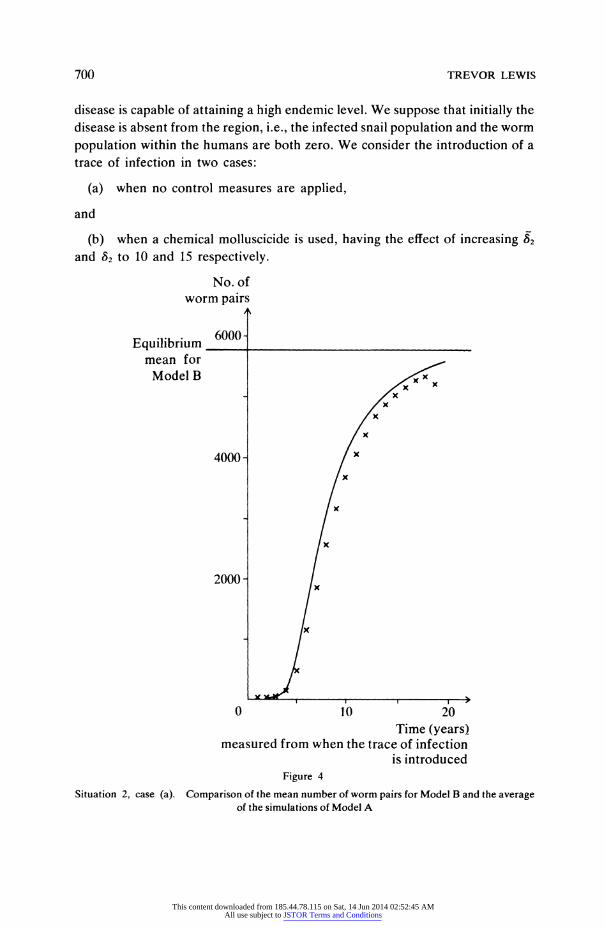
disease is capable of attaining a high endemic level. We suppose that initially the disease is absent from the region, i.e., the infected snail population and the worm
population within the humans are both zero. We consider the introduction of a trace of infection in two cases:
(a) when no control measures are applied,
and
(b) when a chemical molluscicide is used, having the effect of increasing 82
and 82 to 10 and 15 respectively.
No. of worm pairs
6000- Equilibrium
mean for Model B xx
x x
x
4000 -x
x
2000- x
0 10 20 Time (years)
measured from when the trace of infection is introduced
Figure 4
Situation 2, case (a). Comparison of the mean number of worm pairs for Model B and the average of the simulations of Model A
This content downloaded from 185.44.78.115 on Sat, 14 Jun 2014 02:52:45 AMAll use subject to JSTOR Terms and Conditions

A model for the parasitic disease bilharziasis 701
The introduction of a trace of infection is represented by an individual with five pairs of worms.
The results comparing the expected population sizes for Model B and the
average of the simulations of Model A, for the two cases described above, are
given in Figures 4 to 7. From these results it is clear that the increasing of 82 and
82 causes.the
initial conditions to fall below a threshold value which it is
necessary to attain if the disease is to take hold in the region. This idea could have useful applications in restricting the spread of bilharziasis into previously disease-free regions. Again we notice there is good agreement between the mean
No. of infected snails
Equilibrium mean for
Model B x
8000 - x
4000-
0 10 20 Time (years)
measured from when the trace of infection is introduced
Figure 5
Situation 2, case (a). Comparison of the mean number of infected snails for Model B and average of the simulations of Model A
This content downloaded from 185.44.78.115 on Sat, 14 Jun 2014 02:52:45 AMAll use subject to JSTOR Terms and Conditions

702 TREVOR LEWIS
No. of worm pairs
5
4-
x
3-
x
x
2- x
x xxx
x x
0 10 20 Time (years)
measured from when the trace of infection is introduced
Figure 6
Situation 2, case (b). Comparison of the mean number of worm pairs for Model B and the
average of the simulations of Model A
population sizes for Model B and the average of the simulations of Model A. This agreement holds for both the transient behaviour and the endemic level attained. Again we note that the average human population size for the simulations remained close to the equilibrium mean value for Models A and B.
8.3. Summary. Although we have considered just one parameter set and
just one type of control measure, the indications are that Model B is a good approximation to Model A. The greater tractability of Model B allows us to
This content downloaded from 185.44.78.115 on Sat, 14 Jun 2014 02:52:45 AMAll use subject to JSTOR Terms and Conditions

A model for the parasitic disease bilharziasis 703
No. of infected snails
40
30
20 -
x
xX
x xx
xx x
0 10 20 Time (years)
measured from when the trace of infection is introduced
Figure 7
Situation 2, case (b). Comparison of the mean number of infected snails for Model B and the average of the simulations of Model A
study the endemic properties of the disease and the effects of a wide range of control measures.
The simplicity of Equation (7.13) enables us (for certain parameter values) to give good approximations to the endemic levels of the disease and to obtain threshold results concerning the values of these levels. It is hoped that this feature of the model will be investigated in a future paper.
This content downloaded from 185.44.78.115 on Sat, 14 Jun 2014 02:52:45 AMAll use subject to JSTOR Terms and Conditions

704 TREVOR LEWIS
References
ABRAMOWITZ, M. AND STEGUN, I. A. (1965) Handbook of Mathematical Functions. Dover, New York.
BAILEY, N. T. J. (1957) The Mathematical Theory of Epidemics. Griffin, London: Hafner, New York.
COCHRAN, J. A. (1967) The monotonicity of modified Bessel functions with respect to their order. J. Math. Phys. 46, 220-222.
Cox, D. R. AND MILLER, H. D. (1965) The Theory of Stochastic Processes. Methuen, London. DIETZ, K. (1967) Epidemics and rumours: A survey. J. R. Statist. Soc. A 130, 505-528. DIETZ, K. (1972) A supplementary bibliography on mathematical models of communicable
diseases. World Health Organization RECS/72.5. ERDtLYI, A. (1954) Tables of Integral Transforms, Vol. 1. McGraw-Hill, New York. FAROOQ, M. (1967) Progress in bilharziasis control. W.H.O. Chfon. 21, 175-184. HAIRSTON, N. G. (1962) Population ecology and epidemiological problems, in CIBA Foundation
Symposium on Bilharziasis, ed. G. E. W. Wolstenholme and M. O'Connor, pp. 36-62. J. and A. Churchill, London.
JORDAN, P. AND WEBBE, G. (1969) Human Schistosomiasis. W. Heinemann, London.
MACDONALD, G. (1965) The dynamics of helminth infections, with special reference to schistosomes. Trans. Roy. Soc. Trop. Med. Hyg. 59, 489-506.
NASELL, I. AND HIRSCH, W. M. (1971) Mathematical models of some parasitic diseases involving an intermediate host. Report No. IMM393, Courant Institute of Mathematical Sciences, New York.
NASELL, I. AND HIRSCH, W. M. (1973) The transition dynamics of schistosomiasis. Comm. Pure.
Appl. Mtth. 26, 395-453. RALSTON, A. (1965) A First Course in Numerical Analysis. McGraw-Hill, New York. W. H. O. (1965) Monograph Series No. 50. World Health Organization, Geneva.
This content downloaded from 185.44.78.115 on Sat, 14 Jun 2014 02:52:45 AMAll use subject to JSTOR Terms and Conditions