A Model of the monetary system ofMedieval Europe

Angela RedishUniversity of British Columbia

email: angela.redish@ubc.ca

Warren E. Weber∗

Federal Reserve Bank of MinneapolisUniversity of Minnesota

e-mail: wew@minneapolisfed.org

Very preliminaryDO NOT CITE

March 30, 2011

∗We thank Miguel Molico, Francois Velde, Randy Wright, and participants at seminars at theFederal Reserve Bank of Boston, the University of British Columbia, and the University of Oxfordfor helpful comments. The views expressed in this paper are those of the authors and not necessarilythose of the Federal Reserve Bank of Minneapolis or the Federal Reserve System.

“any study of the money supply [of medieval Europe] needs to take account not only ofthe total face value of the currency, but also of the metals and denominations of which it iscomposed.” (Mayhew (2004);82)

The history of commodity money systems is replete with denominational problems. Inmany instances these are complaints of an absence of small denomination coins (a ‘scarcityof small change’) but there were also occasions when there complaints of an absence oflarge denomination media of exchange. The complaints about the absence of small or largedenomination coins reflect the very limited types of coins that circulated in commodity moneysystems. In medieval Europe mints typically produced only one type of coin, a silver pennystamped on both sides, weighing about 1.7 grams and being about 18 mm in diameter. Overthe ensuing centuries pennies continued to be minted, but their silver content and finenessdeclined. Then in the early 13th century, the Italian city states began adding a second cointype, a ‘grosso’ that was very similar to Charlemagne’s penny - of high fineness, but slightlyheavier, around 2 gms. Most other European mints followed suit in the mid 13th century,issuing even larger silver coins even as they continued to mint the penny. In the mid-13thcentury, many mints also began issuing gold coins adding further choices to the coin types.

In this paper we build a model of a commodity money system with a limited number oftypes of coins and show how the choices of coin type influences economic welfare throughthe distribution of wealth and output. We also use the model to show the consequences ofchanges in the stock of the monetary commodity or the extent of trade on the economy. In aprevious paper Redish and Weber (2010) we built a random matching monetary model withtwo indivisible coins and illustrated that a small change shortage could exist in the sense thatadding small coins to the economy with large coins was welfare improving. However, in thatpaper we assumed a fixed quantity of coins of each type and compared the characteristicsof equilibria with different stocks of, and sizes of, coins. The commodity value of the coinswas imposed by assuming that each coin paid a dividend (essentially was a Lucas tree). Inthis paper we endogenize the quantity of money. We assume that there is a fixed stock ofeach monetary metal and allow agents to choose to mint coins (at a cost), or to melt thecoins into jewelry. Thus the model combines a more fundamental way of generating valuedcommodity money, and an endogenous quantity of money (though not quantity of monetarymetal) providing a much richer framework to discuss the shortage of small coins.

Our model is closely related to that of Velde and Weber (2000) and Lee, Wallace, andZhu (2005). ? model a commodity money system allowing agents to hold monetary metalas coins or in a form that yields direct utility - jewelery. The demand for money in theirmodel is driven by a cash-in-advance constraint. Lee, Wallace, and Zhu (2005) build arandom matching model in which agents can hold multiple units of various types of fiatmoney. Agents engage in pair-wise trade alternately with periods where they can rebalancetheir portfolio subject only to a wealth constraint. They prove the existence of a monetarysteady state in which agents trade off the benefits of small denomination notes for transactingagainst their higher handling costs. As in Lee, Wallace, and Zhu (2005) we motivate thedemand for money with a random matching model however, our agents use a commoditymoney and thus there is an additional margin - the marginal utility of jewelry - that bearson how many coins an agent wants to hold.

The paper proceeds as follows: in the next section we describe the types of coinage

1

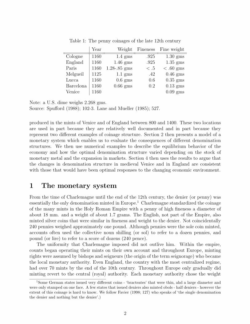
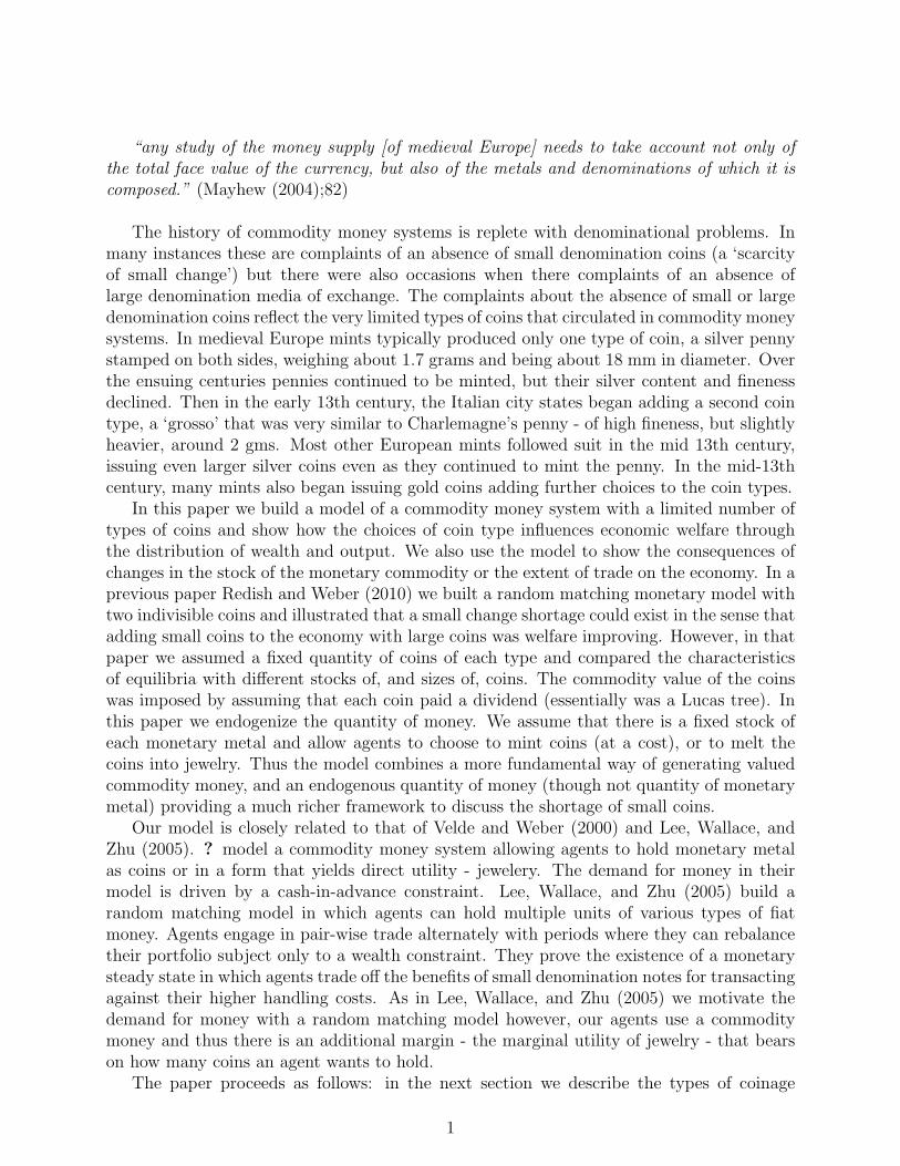
Table 1: The penny coinages of the late 12th century

Year Weight Fineness Fine weight

Cologne 1160 1.4 gms .925 1.30 gmsEngland 1160 1.46 gms .925 1.35 gmsParis 1160 1.28-.85 gms < .5 < .60 gmsMelgueil 1125 1.1 gms .42 0.46 gmsLucca 1160 0.6 gms 0.6 0.35 gmsBarcelona 1160 0.66 gms 0.2 0.13 gmsVenice 1160 0.09 gms

Note: a U.S. dime weighs 2.268 gms.Source: Spufford (1988); 102-3. Lane and Mueller (1985); 527.

produced in the mints of Venice and of England between 800 and 1400. These two locationsare used in part because they are relatively well documented and in part because theyrepresent two different examples of coinage structure. Section 2 then presents a model of amonetary system which enables us to evaluate the consequences of different denominationstructures. We then use numerical examples to describe the equilibrium behavior of theeconomy and how the optimal denomination structure varied depending on the stock ofmonetary metal and the expansion in markets. Section 4 then uses the results to argue thatthe changes in denomination structure in medieval Venice and in England are consistentwith those that would have been optimal responses to the changing economic environment.

1 The monetary system

From the time of Charlemagne until the end of the 12th century, the denier (or penny) wasessentially the only denomination minted in Europe.1 Charlemagne standardized the coinageof the many mints in the Holy Roman Empire with a penny of high fineness a diameter ofabout 18 mm. and a weight of about 1.7 grams. The English, not part of the Empire, alsominted silver coins that were similar in fineness and weight to the denier. Not coincidentally240 pennies weighed approximately one pound. Although pennies were the sole coin minted,accounts often used the collective noun shilling (or sol) to refer to a dozen pennies, andpound (or lire) to refer to a score of dozens (240 pence).

The uniformity that Charlemagne imposed did not outlive him. Within the empire,counts began operating their mints on their own account and throughout Europe, mintingrights were assumed by bishops and seigneurs (the origin of the term seignorage) who becamethe local monetary authority. Even England, the country with the most centralized regime,had over 70 mints by the end of the 10th century. Throughout Europe only gradually didminting revert to the central (royal) authority. Each monetary authority chose the weight

1Some German states issued very different coins - ‘bracteates’ that were thin, ahd a large diameter andwere only stamped on one face. A few states that issued deniers also minted obols - half deniers - however theextent of this coinage is hard to know. We follow Favier (1998; 127) who speaks of ‘the single denominationthe denier and nothing but the denier’.)

2

Table 2: The introduction of new coins, 13th and 14th centuries

Coin Metal Fine weight Value in Silverunit of account equivalent

Venice1172 Denarius Silver .10 gms 1d1201 Grossus Silver 2.1 gms 24d1284 Grossus Silver 2.1 gms 32d1284 Ducat Gold 3.5 gms 576d 50gmsFrance1200 Denier Silver 0.36 gms 1d1266 Gros t Silver 4.2 gms 12d1290 Royale Gold 6.97gms 300d 100 gmsEngland1200 Penny Silver 1.4 gms 1d1279 Farthing Silver .34 gms .25d1344 Noble Gold 8.8 gms 80d 103 gms1351 Groat Silver 4.68 gms 4d

Sources: Lane and Mueller (1985), de Wailly (1857), Challis (1992)

and fineness of the penny that it minted and all diminished both but to very different extents.By 1200 the characteristics of the penny ranged widely (see Table 1) from the English penny,weighing 1.46 gms and 92.5% fine, to the many French coins weighing about 1 gram andabout 35% fine, to the Italian coins that were about one quarter of a gram and less than30% fine (Spufford (1988) p.102-3).

The use of a single type of coin in an economy made payments of both large and smallamounts difficult. In the mid-13th century for example, English agricultural labourers earnedabout 1.6 pence per day and a penny bought for loaves of bread. Throughout Europe theoptions for paying large values were also limited. There were some Byzantine gold coins,particularly in the South of Europe. Silver ingots, stamped with their fineness and oftenweighing an integer number of marks (a mark weighed about 220 grams), were used onoccasion but even for large payments pennies were used, frequently in sealed bags certifiedfor their contents. Spufford (1988) p.210 cites the example of the papal collector for NorthernEurope who collected over 70,000 marks in pence (close to 1 million pence!), as well as over1,000 marks in ingots for remittance to the Pope.

The practice of minting only a single type coin ended in Italy in the last decade of the12th century. In 1190 the Milanese began minting a grosso that was of high fineness andweighed over 2 gms. This coin only circulated locally, but a few years later the Venetiansbegan minting a similar coin which circulated widely. The Venetian grosso contained roughly24 times as much silver as the debased denari that were in circulation. Other mint authoritiesfollowed suit (see Table 2): the French introduced a ‘gros’ in 1266 and the English, a groat in1351.2 In England in contrast, the new denominations that were minted beginning in 1279fractions of a penny: the halfpenny and farthing (quarter penny).

2The mint ordinance of 1279 allowed the minting of groats however numismatists argue that essentially

3

In the late 13th/ early 14th century the denomination structure became yet richer withthe introduction of gold coins, but this still left a large gap in the denomination structure.Because gold is roughly twice as dense as silver (19.3gms/cm3 compared to 10.5gms/cm3)if gold were worth 10 times as much as silver by weight a gold coin of the same size as a 2gm silver coin would be worth 20 times as much. While coining technology was restrictedto hammer and shears the mints were not able to issue very heavy coins. It was not untilscrew presses and rolling mills were introduced into mints in the 16th century, that coins ofup to 30 gms were produced; until then the largest silver coins weighed less than 5 gms.3

The sparse number of coin types led to frequent complaints about the coinage - someconcerning a lack of small change and others of a lack of high value coins and underlies thequotation at the head of the paper.4

2 The Model

2.1 Environment

We build a random matching models in which agents are permitted to hold multiple numbersof each of two types of coins. The model has discrete time and an infinite number of periods.There is a nonstorable, perfectly divisible good and two metals (durable commodities) —silver and gold — in the economy. There are ms ounces of silver and mg ounces of gold inexistence.

The way in which we model commodity money follows that used by Velde and Weber(2000). We assume that silver can be held in either of two forms, which we will refer toas coins and jewelry. Silver held in the form of jewelry yields utility directly to the holder,whereas silver held in the form of coins yields no utility to the holder. Because of difficultiesin determining the weight and fineness of jewelry, we assume that only coins can be traded.There is a utility cost γ of holding a coin. All gold is held as jewelry.5

The technological limitations on minting in the medieval period placed restrictions onwhat the monetary authority could do with coinage. For one, although metals could bedivided, they could be divided only imperfectly. This meant that coins had to be indivisible.Further, coins could not be too small, because of the possibility of loss, and they could notbe too heavy or they would be difficult to carry. The role of the monetary authority inthis environment was to choose how many ounces of metal to put into a coin of that metalsubject to these limitations.

In our model, we allow for the minting of two types of silver coin distinguished by theweight of silver in each coin. We let b1

s be the ounces of silver that it puts in the first silvercoin, and b2

s = ηbs be the amount of silver in the second coin, where η is an integer greater

none were minted between 1279 and 1344; see Section 4.4 below.3Cooper (1988) for the history of coining technology and the limitations it imposed; see ? for discussion

of the coin sizes).4The literature on the scarcity of small change is plagued by confusion between the problem of a ‘scarcity

of small change’ and a ‘want of money’. Here we focus on the denomination question.5Our reason for including gold is that we intend to consider the possible use of gold coins in a later

version of the paper.

4

than one. As was the case with coins throughout most of the time during which commoditymonies were used, these coins do not have denominations. They are simply an amount ofsilver that has been turned into coins with some type of standardized markings that allowone type of coin to be easily differentiated from a different type of coin.

Each period in the model is divided into two subperiods. In the first subperiod agentscan trade in bilateral matches. At the beginning of this subperiod, an agent has a probability12

of being a consumer but not a producer and the same probability of being a producer butnot a consumer. This assumption rules out double coincidence matches, and therefore givesrise to the essentiality of a medium of exchange.

After agents’ types (consumer or producer) are revealed, a fraction θ ∈ (0, 1] of agentsare matched bilaterally. In a match, the portfolios of both agents are known. However, pasttrading histories are private information and agents are anonymous. These assumptions ruleout gift-giving equilibria and the use of credit. Thus, trading can only occur through theuse of media of exchange, which is the role that the gold and silver coins can play.

In the second subperiod, agents can alter their mix of the two types of silver coins andjewelry by minting or melting. That is, in the second subperiod agents can change the formin which they hold the stock of silver, but they cannot change the total quantity in theeconomy.

2.2 Consumer choices

There is a [0, 1] continuum of infinitely lived agents in the model that maximize expecteddiscounted lifetime utility. The discount factor is β. Let c be the quantity of the goodconsumed; q, the quantity of the good produced; and js, the holdings of silver jewelry interms of units of the small coin. The agent’s period preferences are

u(c)− q + µ(b1sjs,mg)

with u(0) = 0, u′ > 0, u′′ < 0, and u′(0) =∞. The disutility of good production is assumedto be linear without loss of generality. We assume that an agent’s utility from holding silverand gold jewelry is µ(bsj

s,mg) with µi > 0, µii ≤ 0.Let s1 and s2 be an agent’s holdings of small and large silver coins, respectively, and .

The agent’s portfolio of metal holdings is

y = (s1, s2, js,mg) : s1, s2, j

s,mg ∈ N.

We assume that in a single coincidence pairwise meeting, the potential consumer gets tomake a take-it-or-leave-it (TIOLI) offer to the potential seller. This offer will be the triple(q, p1, p2), where q ∈ <+ is the quantity of production demanded, pi ∈ Z is the quantity ofsilver coins of type i offered. Offers with p1 < 0 can be thought of as the seller being askedto make change.

Let v(y) : N⊗

N → <+ be the expected value of an agent’s portfolio at the beginningof the second subperiod. The set of feasible TIOLI offers is a combination of special goodoutput and coins that is a feasible coin offer and satisfies the condition that the seller be no

5

worse off than not trading. Denoting this set by Γ(y, y),

Γ(y, y) = (q, p1, p2) : q ∈ <+,−s1 ≤ p1 ≤ s1,−s2 ≤ p2 ≤ s2,

−q + v(s1 + p1, s2 + p2, js, mg) ≥ v(y),

where y denotes the seller’s portfolio. In the second subperiod, the agent can mint or melt.Define zi ∈ Z to be the quantity of silver coins of type i minted (> 0) or melted (< 0).Agents cannot melt more coins than they have, and agents cannot mint in terms of metalmore coins that they have. Note that this does not prevent them from melting coins of onetype and minting coins of the other from the metal gained by melting. Denote the set ofminting and melting choices available to an agent by Ω(y)

Ω(y) = (zs) : zi ≥ −si, z1 + ηz2 ≤ js

Agents can melt coins without incurring a cost. However, if agents mint, they incur aseigniorage cost S(z1, z2; js,mg). To keep the analysis tractable, we will assume that nometal is lost by an agent when minting. Instead, we assume that the seigniorage an agenthas to pay is in terms of utility, but does depend how many coins are minted.

2.3 Equilibrium

The three components needed are the value functions (Bellman equations), the asset transi-tion equations, and the market clearing conditions. We proceed to describe each in turn.

Value functions

Let wt(yt) and vt(yt) be the expected values of holding yt at the beginning of the first andsecond subperiods of period t, respectively. Then the Bellman equation at the beginning ofthe second subperiod is

vt(yt) = max(z1t,z2t)∈Ω(y)

βwt+1(s1t + z1t, s2t + z2t, jst − z1t − ηz2t)− S(z1t, z2t; j

st ,mg)

The Bellman equation at the beginning of the first subperiod is

wt(yt) =θ

2

∑yt

πt(yt) max(qt,p1t,p2t)∈Γ(y,y)

[u(qt) + vt(s1t − p1t, s2t − p2t, jst ,mg)]

+(1− θ

2)vt(yt) + µ(b1

sjst ,mg)− γ(s1t + s2t)

where πt(yt) is the fraction of agents with yt at the beginning of the first subperiod. The firstterm on the right-hand side is the expected payoff from being a buyer in a single coincidencemeeting, which occurs with probability θ

2. The second term is the expected payoff either

from being the seller in a single coincidence meeting or from not have a meeting. The thirdterm is the utility from holding silver jewelry and gold, and the final term is the utility costof carrying silver coins.

6

Asset holdings

Define λb(k, k′; yt, yt) to be the probability that a buyer with yt meeting a seller with yt leaveswith s1 = k, s2 = k′. That is,

λb(k, k′; y, y) =

1 if k = s1 − p1(y, y) and k′ = s2 − p2(y, y)

0 otherwise.

and define λs(k, k′; yt, yt) similarly for the seller.Then the post-trade (pre-mint/melt) asset distribution is

πt(k, k′, js) =

θ

2

∑yt,yt

πt(yt)πt(yt)[λb(k, k′; yt, yt) + λs(k, k′; yt, yt)]

+(1− θ)πt(k, k′, js)

The first term on the right-hand side is the fraction of single coincidence meetings inwhich the buyer leaves with k small silver coins and k′ large silver coins. The second term isthe fraction of such meetings in which the seller leaves with k small silver coins and k′ largesilver coins. The final term is the probability that no meeting occurs, in which case no coinschange hands.

Next define δ(k, k′, h, yt) to be the probability an agent with yt after trade has s1 = k,s2 = k′, and js = h after minting or melting. Then the post-mint/melt (pre-trade nextperiod) asset distribution is

πt+1(k, k′, h) =∑yt

πt(yt)δ(k, k′, h, yt)

Of course, asset holdings must also satisfy∑

y π(y) =∑

y π(y) = 1.

Market clearing

The market clearing condition is that the stock of silver metal must be held. That is,∑y

b1s(s1 + ηs2 + js)π(y) = ms

Definition 1 Steady state equilibrium: A steady state equilibrium is value functionsw, v; asset holdings π and π; and quantities p1, p2, z1, z2, q that satisfy the value functions,the asset transition equations, and market clearing.

This section includes discussion of how fixing the coin size fixes the price level; it alsodiscusses the tradeoff that determines the optimal size of a coin - that is, on the one handsmall coins deliver finer offers and therefore more trade but large coins economize on handlingcosts. If there were no handling costs the optimal single coin size would be very small.

7

3 Results – Single Silver Coin

Because of the long period in which there was only a single silver coin in medieval Europeand to get some intuition about how the model works, we begin by studying our economywhen there is only a single silver coin.

We are unable to prove the existence of steady state equilibria or to obtain analyticresults for even this simple case of our model. Therefore, we rely on computed equilibria fornumerical examples to obtain our results. Specifically, we assume u(q) = q1/4, µ(b1

sjs,mg) =0.05(b1

sjs)1/2 + 0.1581(mg)

1/2, β = 0.9, θ = 23,ms = 0.1,mg = 0.01, and γ = 0.001. Because

we are interested in small change, we will consider various values for bis. Although we havenot attempted to calibrate the parameters in the numerical analysis, the relative weights ofsilver and gold in the jewelry utility function are chosen to approximate the relative marketratio of 1:10 for these metals during the early medieval period.

To avoid problems in keeping track of the quantity of silver in the economy, we defineseigniorage in terms of foregone utility from holding jewelry. Specifically, we assume

S(z1t; jst ,mg) = max[µ(bsj

st ,mg)− µ(bsj

st − bsσsz1t,mg), 0]

where σs is the seigniorage rate. The term µ(bsjst ,mg) is the utility from holding jewelry

before doing any minting. The term µ(bsjst − bsσsz1t,mg) is the utility from holding that

amount of jewelry less the amount of jewelry given up to pay the seigniorage tax on mintingcoins from jewelry. The max with 0 is because seigniorage is only paid on minting. We use aseigniorage rate of σs = 0.04 which was approximately the average seigniorage rate on silverduring this period.

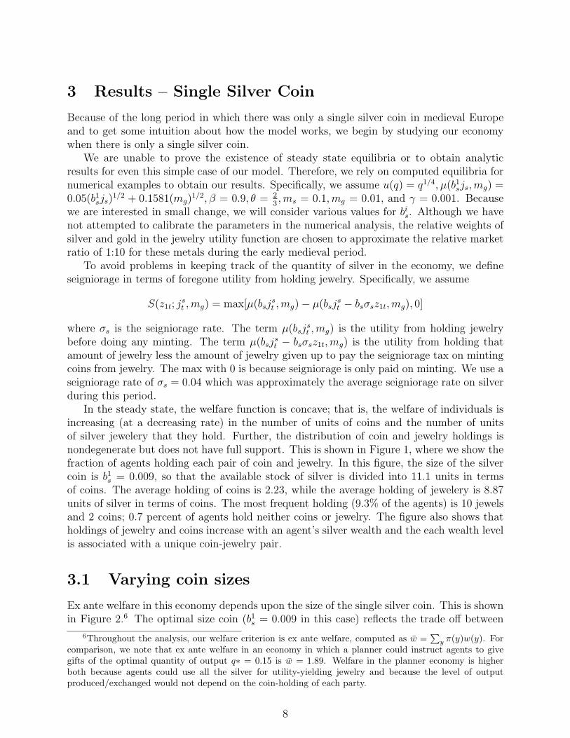
In the steady state, the welfare function is concave; that is, the welfare of individuals isincreasing (at a decreasing rate) in the number of units of coins and the number of unitsof silver jewelery that they hold. Further, the distribution of coin and jewelry holdings isnondegenerate but does not have full support. This is shown in Figure 1, where we show thefraction of agents holding each pair of coin and jewelry. In this figure, the size of the silvercoin is b1

s = 0.009, so that the available stock of silver is divided into 11.1 units in termsof coins. The average holding of coins is 2.23, while the average holding of jewelery is 8.87units of silver in terms of coins. The most frequent holding (9.3% of the agents) is 10 jewelsand 2 coins; 0.7 percent of agents hold neither coins or jewelry. The figure also shows thatholdings of jewelry and coins increase with an agent’s silver wealth and the each wealth levelis associated with a unique coin-jewelry pair.

3.1 Varying coin sizes

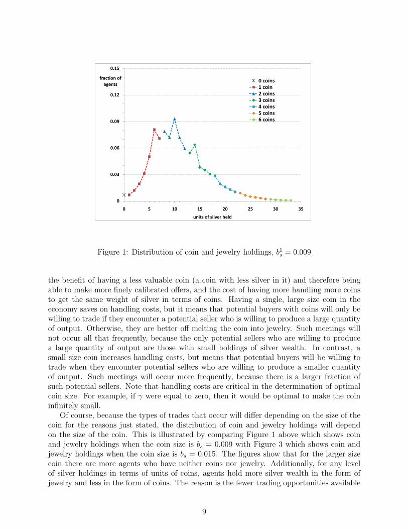
Ex ante welfare in this economy depends upon the size of the single silver coin. This is shownin Figure 2.6 The optimal size coin (b1

s = 0.009 in this case) reflects the trade off between

6Throughout the analysis, our welfare criterion is ex ante welfare, computed as w =∑

y π(y)w(y). Forcomparison, we note that ex ante welfare in an economy in which a planner could instruct agents to givegifts of the optimal quantity of output q∗ = 0.15 is w = 1.89. Welfare in the planner economy is higherboth because agents could use all the silver for utility-yielding jewelry and because the level of outputproduced/exchanged would not depend on the coin-holding of each party.

8

0

0.03

0.06

0.09

0.12

0.15

0 5 10 15 20 25 30 35

fraction ofagents

units of silver held

0 coins1 coin2 coins3 coins4 coins5 coins6 coins

Figure 1: Distribution of coin and jewelry holdings, b1s = 0.009

the benefit of having a less valuable coin (a coin with less silver in it) and therefore beingable to make more finely calibrated offers, and the cost of having more handling more coinsto get the same weight of silver in terms of coins. Having a single, large size coin in theeconomy saves on handling costs, but it means that potential buyers with coins will only bewilling to trade if they encounter a potential seller who is willing to produce a large quantityof output. Otherwise, they are better off melting the coin into jewelry. Such meetings willnot occur all that frequently, because the only potential sellers who are willing to producea large quantity of output are those with small holdings of silver wealth. In contrast, asmall size coin increases handling costs, but means that potential buyers will be willing totrade when they encounter potential sellers who are willing to produce a smaller quantityof output. Such meetings will occur more frequently, because there is a larger fraction ofsuch potential sellers. Note that handling costs are critical in the determination of optimalcoin size. For example, if γ were equal to zero, then it would be optimal to make the coininfinitely small.

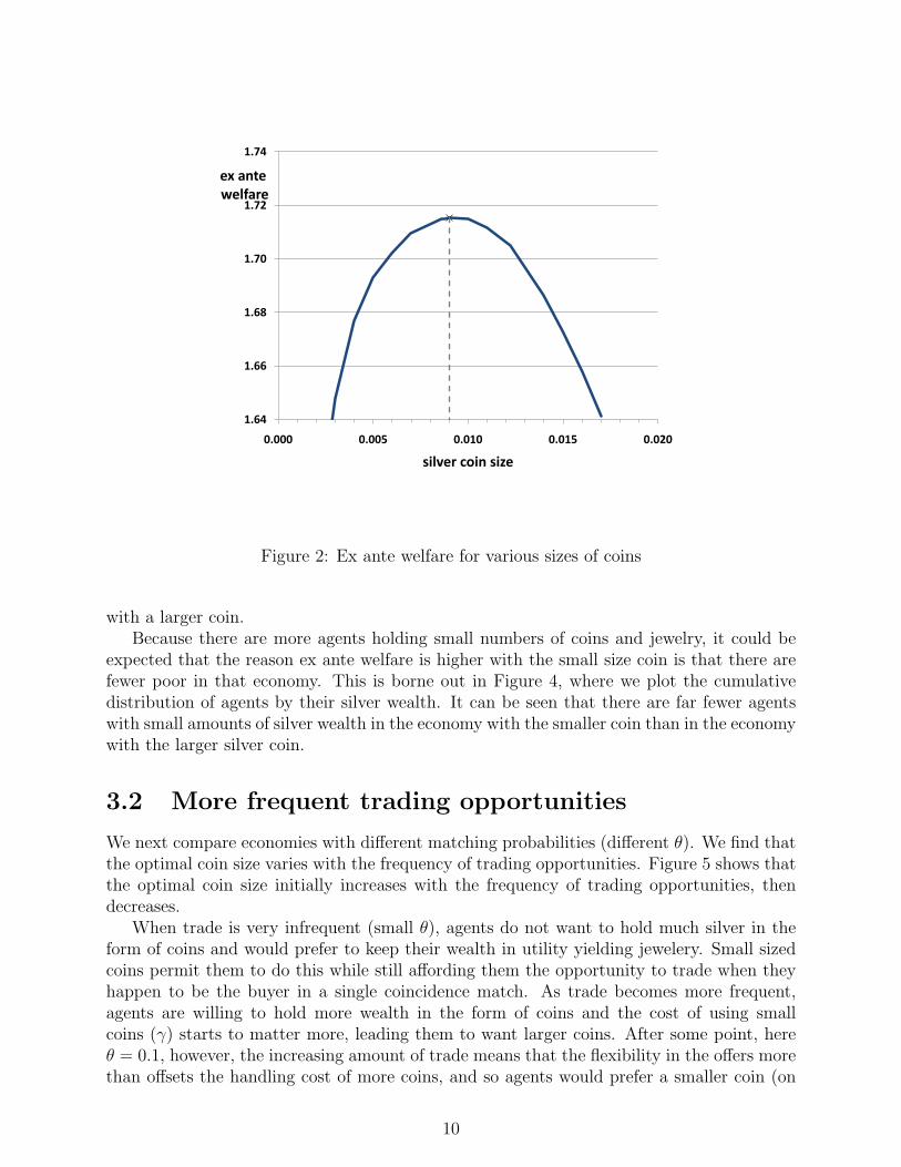
Of course, because the types of trades that occur will differ depending on the size of thecoin for the reasons just stated, the distribution of coin and jewelry holdings will dependon the size of the coin. This is illustrated by comparing Figure 1 above which shows coinand jewelry holdings when the coin size is bs = 0.009 with Figure 3 which shows coin andjewelry holdings when the coin size is bs = 0.015. The figures show that for the larger sizecoin there are more agents who have neither coins nor jewelry. Additionally, for any levelof silver holdings in terms of units of coins, agents hold more silver wealth in the form ofjewelry and less in the form of coins. The reason is the fewer trading opportunities available

9

1.64

1.66

1.68

1.70

1.72

1.74

0.000 0.005 0.010 0.015 0.020

ex antewelfare

silver coin size

Figure 2: Ex ante welfare for various sizes of coins

with a larger coin.Because there are more agents holding small numbers of coins and jewelry, it could be

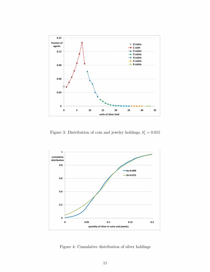
expected that the reason ex ante welfare is higher with the small size coin is that there arefewer poor in that economy. This is borne out in Figure 4, where we plot the cumulativedistribution of agents by their silver wealth. It can be seen that there are far fewer agentswith small amounts of silver wealth in the economy with the smaller coin than in the economywith the larger silver coin.

3.2 More frequent trading opportunities

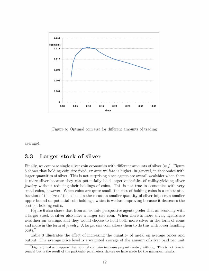
We next compare economies with different matching probabilities (different θ). We find thatthe optimal coin size varies with the frequency of trading opportunities. Figure 5 shows thatthe optimal coin size initially increases with the frequency of trading opportunities, thendecreases.

When trade is very infrequent (small θ), agents do not want to hold much silver in theform of coins and would prefer to keep their wealth in utility yielding jewelery. Small sizedcoins permit them to do this while still affording them the opportunity to trade when theyhappen to be the buyer in a single coincidence match. As trade becomes more frequent,agents are willing to hold more wealth in the form of coins and the cost of using smallcoins (γ) starts to matter more, leading them to want larger coins. After some point, hereθ = 0.1, however, the increasing amount of trade means that the flexibility in the offers morethan offsets the handling cost of more coins, and so agents would prefer a smaller coin (on

10

0

0.03

0.06

0.09

0.12

0.15

0 5 10 15 20 25 30 35

fraction ofagents

units of silver held

0 coins1 coin2 coins3 coins4 coins5 coins6 coins

Figure 3: Distribution of coin and jewelry holdings, b1s = 0.015

0

0.2

0.4

0.6

0.8

1

0 0.05 0.1 0.15 0.2

cumulative distribution

quantity of silver in coins and jewelry

bs=0.009

bs=0.015

Figure 4: Cumulative distribution of silver holdings

11

0

0.003

0.006

0.009

0.012

0.015

0.018

0.00 0.05 0.10 0.15 0.20 0.25 0.30 0.35

optimal bs

theta

Figure 5: Optimal coin size for different amounts of trading

average).

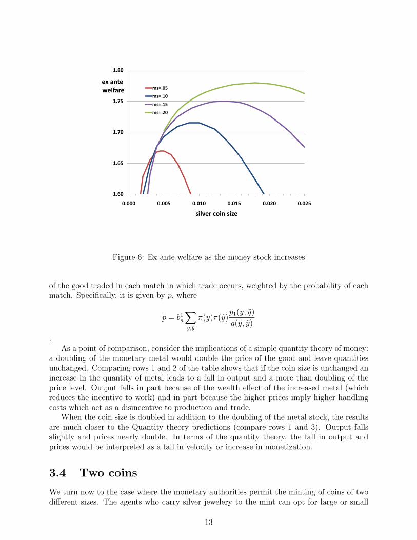
3.3 Larger stock of silver

Finally, we compare single silver coin economies with different amounts of silver (ms). Figure6 shows that holding coin size fixed, ex ante welfare is higher, in general, in economies withlarger quantities of silver. This is not surprising since agents are overall wealthier when thereis more silver because they can potentially hold larger quantities of utility-yielding silverjewelry without reducing their holdings of coins. This is not true in economies with verysmall coins, however. When coins are quite small, the cost of holding coins is a substantialfraction of the size of the coins. In these case, a smaller quantity of silver imposes a smallerupper bound on potential coin holdings, which is welfare improving because it decreases thecosts of holding coins.

Figure 6 also shows that from an ex ante perspective agents prefer that an economy witha larger stock of silver also have a larger size coin. When there is more silver, agents arewealthier on average, and they would choose to hold both more silver in the form of coinsand more in the form of jewelry. A larger size coin allows them to do this with lower handlingcosts.7

Table 3 illustrates the effect of increasing the quantity of metal on average prices andoutput. The average price level is a weighted average of the amount of silver paid per unit

7Figure 6 makes it appear that optimal coin size increases proportionately with ms. This is not true ingeneral but is the result of the particular parameters choices we have made for the numerical results.

12

1.60

1.65

1.70

1.75

1.80

0.000 0.005 0.010 0.015 0.020 0.025

ex antewelfare

silver coin size

ms=.05

ms=.10

ms=.15

ms=.20

Figure 6: Ex ante welfare as the money stock increases

of the good traded in each match in which trade occurs, weighted by the probability of eachmatch. Specifically, it is given by p, where

p = b1s

∑y,y

π(y)π(y)p1(y, y)

q(y, y)

.As a point of comparison, consider the implications of a simple quantity theory of money:

a doubling of the monetary metal would double the price of the good and leave quantitiesunchanged. Comparing rows 1 and 2 of the table shows that if the coin size is unchanged anincrease in the quantity of metal leads to a fall in output and a more than doubling of theprice level. Output falls in part because of the wealth effect of the increased metal (whichreduces the incentive to work) and in part because the higher prices imply higher handlingcosts which act as a disincentive to production and trade.

When the coin size is doubled in addition to the doubling of the metal stock, the resultsare much closer to the Quantity theory predictions (compare rows 1 and 3). Output fallsslightly and prices nearly double. In terms of the quantity theory, the fall in output andprices would be interpreted as a fall in velocity or increase in monetization.

3.4 Two coins

We turn now to the case where the monetary authorities permit the minting of coins of twodifferent sizes. The agents who carry silver jewelery to the mint can opt for large or small

13

Quantity Size of coin Total output Average price Average coinof metal (b1

s) (p holdings

0.1 .009 0.105 0.246 2.040.2 .009 0.087 0.548 4.390.2 .018 0.103 0.458 2.07

Table 3: The effect of doubling the quantity of metal

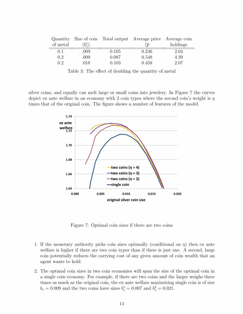
silver coins, and equally can melt large or small coins into jewelery. In Figure 7 the curvesdepict ex ante welfare in an economy with 2 coin types where the second coin’s weight is ηtimes that of the original coin. The figure shows a number of features of the model.

1.64

1.66

1.68

1.70

1.72

1.74

0.000 0.005 0.010 0.015 0.020

ex antewelfare

original silver coin size

two coins (η = 4)

two coins (η = 3)

two coins (η = 2)

single coin

Figure 7: Optimal coin sizes if there are two coins

1. If the monetary authority picks coin sizes optimally (conditional on η) then ex antewelfare is higher if there are two coin types than if there is just one. A second, largecoin potentially reduces the carrying cost of any given amount of coin wealth that anagent wants to hold.

2. The optimal coin sizes in two coin economies will span the size of the optimal coin ina single coin economy. For example, if there are two coins and the larger weighs threetimes as much as the original coin, the ex ante welfare maximizing single coin is of sizebs = 0.009 and the two coins have sizes b1

s = 0.007 and b2s = 0.021.

14

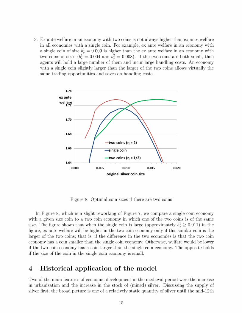
3. Ex ante welfare in an economy with two coins is not always higher than ex ante welfarein all economies with a single coin. For example, ex ante welfare in an economy witha single coin of size b1

s = 0.009 is higher than the ex ante welfare in an economy withtwo coins of sizes (b1

s = 0.004 and b2s = 0.008). If the two coins are both small, then

agents will hold a large number of them and incur large handling costs. An economywith a single coin slightly larger than the larger of the two coins allows virtually thesame trading opportunities and saves on handling costs.

1.64

1.66

1.68

1.70

1.72

1.74

0.000 0.005 0.010 0.015 0.020

ex antewelfare

original silver coin size

two coins (η = 2)

single coin

two coins (η = 1/2)

Figure 8: Optimal coin sizes if there are two coins

In Figure 8, which is a slight reworking of Figure 7, we compare a single coin economywith a given size coin to a two coin economy in which one of the two coins is of the samesize. The figure shows that when the single coin is large (approximately b1

s ≥ 0.011) in thefigure, ex ante welfare will be higher in the two coin economy only if this similar coin is thelarger of the two coins; that is, if the difference in the two economies is that the two coineconomy has a coin smaller than the single coin economy. Otherwise, welfare would be lowerif the two coin economy has a coin larger than the single coin economy. The opposite holdsif the size of the coin in the single coin economy is small.

4 Historical application of the model

Two of the main features of economic development in the medieval period were the increasein urbanization and the increase in the stock of (mined) silver. Discussing the supply ofsilver first, the broad picture is one of a relatively static quantity of silver until the mid-12th

15

century. In approximately 1160 the discovery and exploitation of silver mines at Freibergproduced a significant increase in the quantity of silver.8 Indeed, Spufford (1988) titled therelevant chapter of his seminal monetary history of medieval Europe “New silver, c.1160-1320”. The new silver found its way first to the Italian cities the most commercialized andtrade-oriented part of the continent, and particularly to Venice the nearest city to the mines(Lane and Mueller (1985) 138). By the early 14th century, the silver had made its waythroughout Europe. Spufford (2002); 12) estimates that in 1319 there were 800 tons of silvercoin circulating in England, ”a twenty-fourfold increase since the mid-twelth century”.

Economic historians have described the ”renaissance of markets” between the 10th and13th centuries in Europe, as a process that spread intermittently beginning in Northern Italyand gradually spreading to the Low Countries, France and England (e.g. Epstein (2009)ch.4). Venice benefitted from its Maritime position and profited from acting as an entrepotfor trade with the Levant and as the city grew richer it attracted a greater population. Theacceleration of commercial activity and urbanization in England came perhaps a centurylater in England reflecting and stimulating the growth of the wool trade. In this section, weexamine the impact of these changes through the lens of our monetary model.

4.1 Gradual debasement of the Italian coinage

Between 800 and 1150, the silver content of the denarius minted in the various Italian citystates fell from about 1.7 gms to roughly .05 grams. This debasement is often blamed onthe greed of monetary authorities. However, historians of Venice in this period have viewedthe debasement as a reasonable response to economic expansion that exceeded the growthof monetary metal. For example, Cipolla (1963) argued that the dramatic growth of theItalian population between the mid-9th and mid-13th centuries and simultaneous increaseint he division of labor significantly increased the demand for money. He argued (p.417)that the “inelastic supply of precious metals which did not expand proportionately to theincrease in the demand for money [created circumstances such that] if prolonged deflationarypressure and a dangerous downward movement of prices were to be avoided” debasement ofthe denarius was necessary. Notice that the ‘dangerous’ deflation is a fall in prices measuredin denari not in ounces of silver. He accepts that debasement would not avert a fall in theprices of goods in silver. Also note that while Cipolla argues that the supply of preciousmetal was inelastic, he discusses the availability of metal through trade rather than the othermargin which was closer to home, the undoubted availability of silver in the form of plate.

In our model, the increase in trading is best captured by an increase in θ, and the modelimplies that in an economy with more trade there are benefits from a coin with less silver(e.g. from a debasement of the penny) in order that there are more coins in circulationand that each coin’s value has decreased. As shown in Figure 5 (above some thresholdlevel of economic activity) the optimal coin size decreases with increasing trade: producingmore coins from a given quantity of metal by making smaller coins does bring an increasein handling costs, but the benefit of being able to make finer offers outweighs these costs.

8As the numismatists and historians note while rough measures of the quantity of mined can be estimated,the initial stock is not known. The conclusion as to the significance of the increase in part rests on theanecdotal discussion of contemporaries and on the change in volume of activity at mints.

16

This mechanism is analagous to the argument that Lane and Mueller (1985) makes for thedebasement of the penny. They suggest (p.25) that the ‘growing need for coin that arose fromthe increased use of markets and the general expansion of trade’ implied that debasementwas ‘in the public interest’. In practice, the amount of silver in a coin could be reduced bymaking a lighter coin or a lower fineness coin.

4.2 Venice introduces the grosso

The era of the penny ended in the last decade of the 12th century when the Venetiansintroduced the grosso, a silver coin reminiscent of the Carolingian penny, weighing just over2 gms and being over 95% fine. The Venetian denarius by that time contained about a twelthof a gram of pure silver and was about 25% fine, so that the grosso was worth about 24d.

The traditional explanation for the introduction of the grosso attributes it to the needfor a convenient coin to facilitate buying materials and paying wages for outfitting a fleet forthe Fourth Crusade in 1200 AD.9 More recently, Lane and Mueller (1985) and Stahl (2000)have provided evidence that the coin was actually introduced in the early 1190s, that is,before the needs of the Crusade. Lane and Mueller (1985) (p.114) note, however, that thesuccess of the grosso was assisted by the massive inflow of silver provided for outfitting thefleet, enough to mint 4 million grossi. The increasing production of German silver mines(and the importance of Venice as an entrepot for trade with the Levant) provided a furtherinflux of silver.

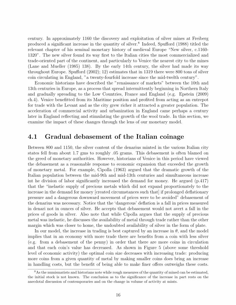
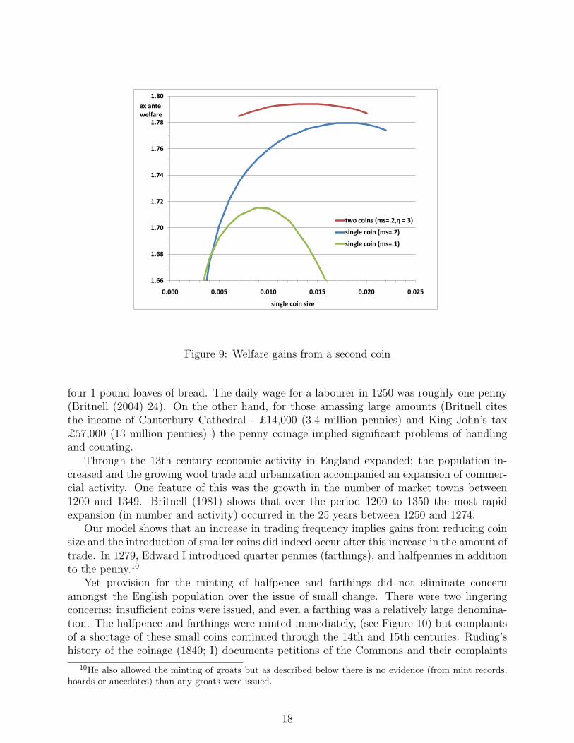
As noted in Section 3.4 for our baseline economy, welfare is always higher if there aretwo coins in the economy relative to only having the smaller of the two coins. That said,the model does highlight the importance of the amount of available silver in motivating theprovision of a large coin. Figure 9 compares the welfare gains from adding a second coin ineconomies with different amounts of monetary metal. In both cases there are gains from thesecond coin. However, consider a monetary authority that wished to add a second coin threetimes as large to a single coin with b1

s = 0.009. When the metal stock is 0.1 the welfare gainsare modest, but when the metal stock is larger, the second coin adds much greater benefits.

4.3 England’s introduction of farthings and halfpence

In contrast to the debasement of the penny in the Italian city states, the weight and fine-ness of the English penny declined very little from 800 to 1150. (See Table 1). By 1200when relatively advanced Venice introduced the grosso as a large silver coin, the only coinbeing minted in England was still the penny, worth about three-quarters of a grosso. Theinconvenience of the penny for day-to-day life is apparent from the prices of bread and ale,the two most common household purchases. A penny would buy 9 or 10 gallons of ale or

9Grierson (1979) makes this case and it is repeated, for example, in Spufford (1988). While Lane andMueller (1985) argue that the introduction of the grosso preceded the Crusaders needs they also suggest thatthe grosso would have been a convenient coin for paying the workmen involved: weekly wages of 144d wouldbe more easily counted out as 5 grossi and 14 denari. In his later history of medieval coinage Grierson (1991;105) notes that “ [ the grossi] simplified and speeded up commercial transactions by reducing the number ofcoins involved in payments”.

17

1.66

1.68

1.70

1.72

1.74

1.76

1.78

1.80

0.000 0.005 0.010 0.015 0.020 0.025

ex antewelfare

single coin size

two coins (ms=.2,η = 3)

single coin (ms=.2)

single coin (ms=.1)

Figure 9: Welfare gains from a second coin

four 1 pound loaves of bread. The daily wage for a labourer in 1250 was roughly one penny(Britnell (2004) 24). On the other hand, for those amassing large amounts (Britnell citesthe income of Canterbury Cathedral - £14,000 (3.4 million pennies) and King John’s tax£57,000 (13 million pennies) ) the penny coinage implied significant problems of handlingand counting.

Through the 13th century economic activity in England expanded; the population in-creased and the growing wool trade and urbanization accompanied an expansion of commer-cial activity. One feature of this was the growth in the number of market towns between1200 and 1349. Britnell (1981) shows that over the period 1200 to 1350 the most rapidexpansion (in number and activity) occurred in the 25 years between 1250 and 1274.

Our model shows that an increase in trading frequency implies gains from reducing coinsize and the introduction of smaller coins did indeed occur after this increase in the amount oftrade. In 1279, Edward I introduced quarter pennies (farthings), and halfpennies in additionto the penny.10

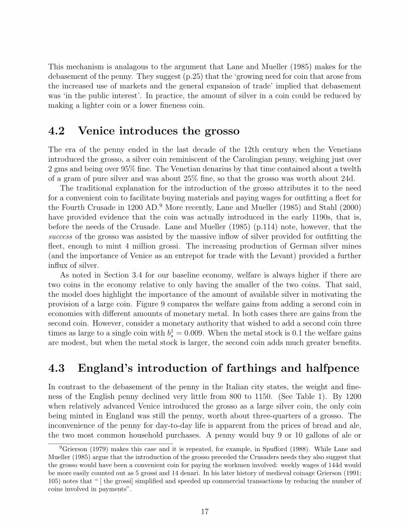
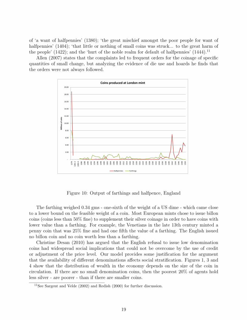
Yet provision for the minting of halfpence and farthings did not eliminate concernamongst the English population over the issue of small change. There were two lingeringconcerns: insufficient coins were issued, and even a farthing was a relatively large denomina-tion. The halfpence and farthings were minted immediately, (see Figure 10) but complaintsof a shortage of these small coins continued through the 14th and 15th centuries. Ruding’shistory of the coinage (1840; I) documents petitions of the Commons and their complaints

10He also allowed the minting of groats but as described below there is no evidence (from mint records,hoards or anecdotes) than any groats were issued.

18

of ‘a want of halfpennies’ (1380); ‘the great mischief amongst the poor people for want ofhalfpennies’ (1404); ‘that little or nothing of small coins was struck... to the great harm ofthe people’ (1422); and the ‘hurt of the noble realm for default of halfpennies’ (1444).11

Allen (2007) states that the complaints led to frequent orders for the coinage of specificquantities of small change, but analyzing the evidence of die use and hoards he finds thatthe orders were not always followed.

-

2.00

4.00

6.00

8.00

10.00

12.00

14.00

16.00

18.00

20.00

12

79

12

81

-2

12

83

-4

12

86

12

88

12

90

12

92

12

94

12

96

12

98

13

00

13

02

13

04

13

06

13

08

13

10

13

12

13

14

13

16

13

18

13

20

13

22

13

24

13

26

13

28

13

30

13

32

13

34

13

36

13

38

13

40

13

42

13

44

13

46

13

48

13

50

Mill

ion

s o

f co

ins

Coins produced at London mint

Halfpennies Farthings

Figure 10: Output of farthings and halfpence, England

The farthing weighed 0.34 gms - one-sixth of the weight of a US dime - which came closeto a lower bound on the feasible weight of a coin. Most European mints chose to issue billoncoins (coins less than 50% fine) to supplement their silver coinage in order to have coins withlower value than a farthing. For example, the Venetians in the late 13th century minted apenny coin that was 25% fine and had one fifth the value of a farthing. The English issuedno billon coin and no coin worth less than a farthing.

Christine Desan (2010) has argued that the English refusal to issue low denominationcoins had widespread social implications that could not be overcome by the use of creditor adjustment of the price level. Our model provides some justification for the argumentthat the availability of different denominations affects social stratification. Figures 1, 3 and4 show that the distribution of wealth in the economy depends on the size of the coin incirculation. If there are no small denomination coins, then the poorest 20% of agents holdless silver - are poorer - than if there are smaller coins.

11See Sargent and Velde (2002) and Redish (2000) for further discussion.

19

4.4 England’s groat issues

Seventy years later, in 1351, Edward III ordered the coining of groats - a coin containing asmuch silver as four pence (as well as the existing silver denominations and a half groat).12

The 1279 legislation had permitted the issue of groats but none had been minted, however,after 1351 a large numbers of groats were issued (Allen (2007)).

The failure of the groat in 1279 and its subsequent popularity after 1351 prompted PeterSpufford (1988; 234) to pose the question “What conditions determined the readiness of anarea for the use of coins of a larger denomination than the penny?” He concludes that the keyfactor was the number and pay rate of urban wage-earners and soldiers. Between 1280 and1350 the urban population of England increased, as did the wage rate: wages for a buildinglaborer in the 1280s were about 9d. weekly, and in 1351 had risen to about 18d weekly. ForSpufford, “In 18d weekly pay, a groat was marginally acceptable”.

In the context of our model, the urban pay explanation seems incomplete. Workers weretypically paid daily and wages of 11

2d/day don’t seem to make groats an ideal medium.

Studies of the ’scarcity of small change’ such as Sargent and Velde (2002) cite frequentcomplaints about a lack of small change, particularly to buy bread and beer - the staple dietof the building-laborers.13

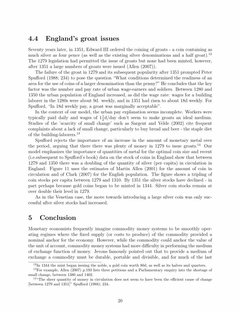
Spufford rejects the importance of an increase in the amount of monetary metal overthe period, arguing that there there was plenty of money in 1279 to issue groats.14 Ourmodel emphasizes the importance of quantities of metal for the optimal coin size and recent(i.e.subsequent to Spufford’s book) data on the stock of coins in England show that between1279 and 1350 there was a doubling of the quantity of silver (per capita) in circulation inEngland. Figure 11 uses the estimates of Martin Allen (2001) for the amount of coin incirculation and of Clark (2007) for the English population. The figure shows a tripling ofcoin stocks per capita between 1279 and 1310. By 1351 the silver stocks have declined - inpart perhaps because gold coins began to be minted in 1344. Silver coin stocks remain atover double their level in 1279.

As in the Venetian case, the move towards introducing a large silver coin was only suc-cessful after silver stocks had increased.

5 Conclusion

Monetary economists frequently imagine commodity money systems to be smoothly oper-ating regimes where the fixed supply (or costs to produce) of the commodity provided anominal anchor for the economy. However, while the commodity could anchor the value ofthe unit of account, commodity money systems had more difficulty in performing the mediumof exchange function of money. Jevons famously pointed out that to provide a medium ofexchange a commodity must be durable, portable and divisible, and for much of the last

12In 1344 the mint began issuing the noble, a gold coin worth 80d, as well as its halves and quarters.13For example, Allen (2007) p.193 lists three petitions and a Parliamentary enquiry into the shortage of

small change, between 1380 and 1402.14“The sheer quantity of money in circulation does not seem to have been the efficient cause of change

[between 1279 and 1351]” Spufford (1988); 234.

20

Sources: Allen (EHR, 2001); Clark (EHR, 2007)

0

10

20

30

40

50

60

70

80

90

100

1200 1250 1300 1350 1400 1450 1500

Pe

nce

pc

Coins stocks per capita, England

Figure 11: Value of coins stocks per capita, England

millennium gold and silver were adopted as monetary commodities because they had suchqualities. Identifiability (for example, of the purity of the metal in a coin) and uniformity(permitting payments to be made by tale rather than by weight) were further desirable char-acteristics of money. The desire for these attributes promoted the use of coined metals andthe monopolization of the right to mint coins. In turn, the monopoly production of coinsgave the monetary authority (typically the Crown) two instruments of monetary policy: therate of seignorage and the size of coins - the denomination structure.

Monetary historians have documented the difficulties created by these monetary systemsand argued that denominational structures are an important contributor to those difficulties.In this paper we construct a model of a monetary economy in which a commodity can beused to produce an indivisible coin that can be used for transactions.

We use the model to analyze the implications of alternative monetary policy choices. Inparticular, we examine the impact of the denomination structure on welfare, and find thatthere is an optimal denomination structure. We show that as the trading opportunities risethe optimal size of the silver coins shrinks, and that as the stock of the monetary commodityrises the optimal size of the coin increases. We then document some examples of changingdenomination structure in medieval Europe and use the model to show how changes in theeconomic environment would have influenced the economically efficient coin types.

21

Bibliography

Allen, M. (2001): “The volume of the English currency, 1158-1470,” Economic historyreview, 54(4), 595–611.

(2007): “The Proportions of the Denominations in English mint outputs, 1351-1485,” British Numismatic Journal.

Britnell, R. (1981): “The proliferation of markets in England, 1200-1349,” EconomicHistory Review, 34(2), 209–221, New Series.

Britnell, R. (2004): “Uses of Money in Medieval England,” in Medieval Money Matters,ed. by D. Wood, pp. 16–30. Oxbow Books, Oxford, England.

Challis, C. (1992): A New History of the Royal Mint. Cambridge University Press, Cam-bridge.

Cipolla, C. (1963): “Curency Depreciation in Medieval Europe,” Economic History Re-view, 15(3), 413–422, New Series.

Clark, G. (2007): “The Long March of History, Farm wages, population and economicGrowth, England, 1209-1869,” Economic History Review, 60(1), 97–135, New Series.

Cooper, D. (1988): The Art and Craft of Coin making: a history of minting technology.Spink and son, London, UK.

de Wailly, N. (1857): Memoire sur les Variations de la livre Tournoise depuis la regne deSaint Louis jusqu’a l’etablissment de la monnaie decimale, vol. 1. Johns Hopkins UniversityPress, Baltimore, Coins and Moneys of Account.

Desan, C. (2010): “The social stratigraphy of coin and credit in late medieval England,”paper presented at ”the Medieval World of Value” conference, Harvard Institute for GlobalLaw and Policy, May 2010.

Epstein, S. (2009): The Economic and Social History of Later Medieval Europe. Universityof Cambridge Press, New York.

Grierson, P. (1979): “The origins of the grosso and of gold coinage in Italy,” in Later Me-dieval Numismatics, ed. by P. Grierson, pp. 72–86. Variorum Reprints, London, England.

Lane, F., and R. Mueller (1985): Money and Banking in Medieval and RenaissanceVenice, vol. 1. Johns Hopkins University Press, Baltimore, Coins and Moneys of Account.

Lee, M., N. Wallace, and T. Zhu (2005): “Modeling Denomination Structures,” Econo-metrica, 73(3), 949–960.

Mayhew, N. J. (2004): “Coinage and Money in England, 1086–c.1500,” in Medieval MoneyMatters, ed. by D. Wood, pp. 72–86. Oxbow Books, Oxford, England.

Redish, A. (2000): Bimetallism: An economic and historical analysis. Cambridge Univer-sity Press, Cambridge, UK.

22

Redish, A., and W. Weber (2010): “Coin sizes and payments in Commodity moneysystems,” .

Sargent, T. J., and F. R. Velde (2002): The Big Problem of Small Change. PrincetonUniversity Press, Princeton, NJ.

Spufford, P. (1988): Money and its use in medieval Europe. Cambridge University Press,Cambridge, England.

Spufford, P. (2002): Power and Profit: The Merchant in Medieval Europe. Thames andHudson, London, UK.

Stahl, A. (2000): Zecca: The mint of Venice in the Middle Ages. Johns Hopkins UniversityPress, Baltimore.

Velde, F. R., and W. E. Weber (2000): “A Model of Bimetallism,” Journal of PoliticalEconomy, 108(6), 1210–1234.

23