A modied seasonal cycle during MIS31 superinterglacialfa ... · The understanding of the air-sea interaction related to the equatorial Pacic and its climate response at interannual

A modified seasonal cycle during MIS31 superinterglacial favorsstronger ENSO variabilityFlavio Justino1, Fred Kucharski2, Douglas Lindemann1, Aaron Wilson3, and Frode Stordal4

1Department of Agricultural Engineering, Universidade Federal de Vicosa, PH Rolfs, Vicosa, Brazil2The Abdus Salam International Centre for Theoretical Physics, Trieste, Italy3Polar Meteorology Group, Byrd Polar and Climate Research Center, The Ohio State University, Columbus, OH, USA4University of Oslo,Department of Geosciences, Forskningsparken Gaustadalleen, Oslo, Norway

Correspondence: Flavio Justino ([email protected])

Abstract. It has long recognized that the amplitude of the seasonal cycle can substantially modify climate features in distinct

timescales. This study evaluates the impact of enhanced seasonality characteristic of the Marine Isotope Stage 31 (MIS31) on

the El Niño-Southern Oscillation (ENSO). Based upon coupled climate simulations driven by present day (CTR) and MIS31

boundary conditions, we demonstrated that the CTR simulation shows signicant concentration of power in the 3-7 year band

and on the multidecadal time scale between 15-30 years. However, the MIS31 simulation shows drastically modified temporal5

variability of the ENSO, with stronger power spectrum at interannual time scales but absence of the decadal periodicity.

Increased meridional gradient of SST and wind stress in the Northern Hemisphere subtropics, in concert with weaker seasonal

cycle of the windstress in the MIS31 simulation, revealed to be the primary candidates responsible for changes in the equatorial

variability. The oceanic response to the MIS31 ENSO extends to the extratropics, and fits nicely with SST anomalies delivered

by paleoreconstructions. The implementation of the MIS31 conditions results in distinct global monsoon system and its link10

to the ENSO in respect to current conditions. In particular, the Indian monsoon intensified but no correlation with ENSO is

found in the MIS31 climate, diverging from conditions delivered by our current climate in which this monsoon is significatly

correlated with the NINO34 index. This indicates that monsoonal precipitation for this interglacial is more closely connected

to hemispherical features than to the tropical-extratropical climate interaction.

1

Clim. Past Discuss., https://doi.org/10.5194/cp-2018-150Manuscript under review for journal Clim. PastDiscussion started: 26 November 2018c© Author(s) 2018. CC BY 4.0 License.

1 Introduction

The Marine Isotope Stage 31 (MIS31; early Pleistocene 1085-1055 ka) is a prime paleoclimate period to simulate and analyze

the global environmental response to a significantly modified climate forcing (Lisiecki and Raymo, 2005; Yin and Berger,

2012a). This interval was characterized by boreal summer temperatures that were several degrees greater than modern climate,

with a substantial recession of the Northern Hemisphere (NH) sea ice (Melles etal., 2012; Justino etal., 2017).5

On long time scales, Earth’s climate is primarily controlled by external and internal processes related to the astronomical

forcing and the atmospheric concentration of greenhouse gases (Stocker etal., 2013; Erb etal., 2015). Internal modes of climate

variability, such as the El Niño-Southern Oscillation (ENSO), the Pacific Decadal Oscillation (PDO) and the Northern Annular

Mode (NAM), also induce climate anomalies on interannual and decadal time scales (Bjerknes, 1964; Mantua etal., 1997;

Thompson and Wallace, 2001). Indeed, changes in the physical and dynamical characteristics of the ENSO have been related10

to seasonal and interannual global-climate distubances (Cai etal., 2014).

The impact of equatorial dynamics and ENSO have been found in different equilibrium climates forced by glacial and inter-

glacial conditions (Karamperidou etal., 2015). For instance, palaeoreconstructions have demonstrated a significant reduction in

the climate variability associated with ENSO during the mid-Holocene (≈ 6000 years before present (BP); Karamperidou etal.

(2015)). The glacial maximum climate was affected by distinct ENSO variability as well; however, during this time the15

ENSO demonstrated larger-amplitude self-sustained interannual variations compared to current conditions (Tudhope etal.,

2001; An etal., 2004; Toniazzo, 2006; Zhu etal., 2017).

Larger differences in the east-west SST gradient in the equatorial Pacific that began 1.17 million years ago, has also been

claimed to support the onset and intensification of the modern Walker circulation (McClymont and Rosell-Melé, 2005). How-

ever, it can be argued that there is no a preferential dominant region in the equatorial Pacific, because global climate distur-20

bances have been found in response to NIÑO3, NIÑO4 or NIÑO34 anomalies. For instance, Yin etal. (2014) indicates that

warmer conditions during the MIS13, an interglacial that occured at approximately 0.5 million years ago, in the Indian-Pacific

warming pool, amplifies the insolation effect and contributes to a large increase of summer precipitation in southern China,

whereas dryer conditions occur in northern China.

The far-reaching effect of equatorial dynamics on climate has been demonstrated by Karami etal. (2015). They argued that25

colder summer sea surface temperatures (SSTs) in the central tropical Pacific during MIS13 contributes to the strengthening

of the northern Pacific subtropical high, increasing the transport of moisture into the East Asia Summer Monsoon (EASM).

Moreover, they highlight the significant influence of the east-west SST differences in the tropical Pacific in maintaining the

link between the tropical Pacific and EASM.

(Sun etal., 2010b) based on seven million years of wind and precipitation variability on the Chinese Loess Plateau, demon-30

strated that monsoonal fluctuations at orbital-to-millennial scales is dynamically linked to changes in solar insolation and in-

ternal boundary conditions, which are tightly related to interglacial ENSO variability. Additional analyses by Rachmayani etal.

(2016) demonstrated that the global monsoon system during interglacial stages differs from current conditions, which may be

characterized by the out-of-phase between the West African and Indian monsoon.

2


Significantly modified periodicity and amplitude of past ENSO regimes and their global influence, shed light on the potential

effect of human induced climate change on the equatorial Pacific, and consequently on future ENSO-like climate. Furthermore,

it should be argued that disagreement in the magnitude of cooling or warming among coupled climate models and paleorecon-

structions may be related to the local responses of temperature and precipitation elicited by distinct ENSO (Peltier and Solheim,5

2004; Jost etal., 2005; Yin and Berger, 2012b; Dolan etal., 2015; Justino etal., 2017).

The effect of ocean dynamics also modify the tropical-polar interaction due to different ENSO flavors (Wilson etal., 2014,

2016), that through changes in the atmospheric circulation can result in anomalous sea-ice/ice sheet mass characteristics

(Steig etal., 2013). The warmer climate of the MIS31 has been shown to result in an overall reduction of snow cover that

to some extent, may be similar to estimates based on simulations of human-induced future global warming (Frei and Gong,10

2005).

The understanding of the air-sea interaction related to the equatorial Pacific and its climate response at interannual and

multi-decadal timescales in distict epochs, such as interglacial intervals, is therefore crucial. It is also vital to understand past

interglacial intervals that are characterized by depleted ice sheets to verify the potential effects of increasing atmospheric CO2,

as the stability of the West Antarctic Ice Sheet (WAIS) will be a key climate factor in decades to come (Nicolas etal., 2017).15

2 Coupled Climate Simulations

Two model simulations have been performed with the International Centre for Theoretical Physics - Coupled Global Climate

Model (ICTP-CGCM; Kucharski etal., 2016). ICTP-CGCM consists of the atmospheric global climate model "SPEEDY"

version 41 (Kucharski etal., 2006) coupled to the Nucleus for European Modelling of the Ocean v3.3 (NEMO) model (Madec,

2008) with the OASIS3 coupler (Valcke, 2013).20

The atmospheric component runs at T30 horizontal resolution, and there are eight levels in the vertical. NEMO is a primitive

equation z-level ocean model based on the hydrostatic and Boussinesq approximations. This version applies a horizontal

resolution of 2◦ and a tropical refinement to 0.5◦. The ocean component has 31 vertical levels with layer thicknesses ranging

from 10 m at the surface to 500 m at the ocean bottom (16 levels in the upper 200 m). Additional details on the ICTP-CGCM

coupled model are discussed by Justino etal. (2017). Farneti etal. (2014) used the ICTP-CGCM to examine the interaction25

between the tropical and subtropical northern Pacific at decadal time scales, suggesting that extratropical atmospheric responses

to tropical forcing have feedbacks onto the ocean dynamics leading to a time-delayed response of the tropical oceans.

Two simulations are evaluated: the modern climate driven by present-day boundary conditions (CTR) and a second ex-

periment for the MIS31 forcing (see Fig. 1 of supplementary material by Justino etal. (2017). The CTR (MIS31) simulation

was run to equilibrium for 2000 (1000) years and the analyses discussed herein are based on the last 500 years of each sim-30

ulation. The MIS31 run starts from equilibrated CTR conditions, including modifications of the WAIS topography based on

Pollard and DeConto (2009), and the planetary astronomical configuration of 1.072 Ma according to Coletti etal. (2014).

The implementation of MIS31 Antarctic topography differs from the CTR counterpart primary by the absence of the WAIS,

which according to Pollard and DeConto (2009), was induced by changes in ocean melt via the effect on ice-shelf buttressing

3


that coincides with strong boreal summer insolation anomalies. In all experiments, the CO2 concentration was set to 325 ppm

which is based on boron isotopes in planktonic foraminifera shells for the MIS31 interval (Honisch etal., 2009). The MIS31

and CTR experiments have been described in further detail elsewhere by Justino etal. (2017), but a brief discussion of the5

global climate differences between these two runs are provided below.

Table 1 shows the global and hemispheric surface temperature values for the CTR and MIS31 simulations, HadCRUT4

(Morice etal., 2012) for the base period 1961-1990 and ERA-Interim (ERA-I; Dee etal., 2011) for the 1980-2010 interval. Our

CTR climate is warmer than the HadCRUT4 and ERA-I but better correspondence is found with the ERA-I. Larger differences

are noticed for the NH summer when the CTR climate is 2◦C (1◦C) warmer than HadCRUT4 (ERA-I). These differences10

arise from higher temperatures over land, because the SST and sea-ice distributions in the CTR simulation fit well with the

ERA-I dataset, as shown by Justino etal. (2017). Temperature differences between the MIS31 and the CTR show that most

of warming occurs in the boreal summer, reaching 1.2◦C in the global mean, 2.2◦C in the NH, and 0.4◦C in the Southern

Hemisphere (SH). Lower temperatures are demonstrated during DJF in the MIS31 run compared to the CTR simulation,

clearly showing the hemispheric seesaw effect of the astronomical forcing.15

Due to astronomically driven reduced seaice, larger changes are located in the NH extratropics (see Justino etal. (2017)). It

has to be mentioned that differences between the MIS31 and CTR simulation deliver negative surface temperature anomalies

over southern Asia, western equatorial Pacific and South Atlantic. Compared to tropical and extratropical paleoreconstructions,

the MIS31 simulation performs well with values that departure from paleoproxies by ± 1◦C in the tropics between 20◦N-3◦S

(McClymont and Rosell-Melé, 2005; Medina-Elizalde etal., 2008; Herbert etal., 2010b, c; Li etal., 2011; Russon etal., 2011;20

Dyez and Ravelo, 2014) by up to -3◦C within 41-67◦N belt (Raymo etal., 1996; Herbert etal., 2010a; Li etal., 2011; Naafs etal.,

2013) and± 1.5◦C in the SH between 23-42◦S (McClymont etal., 2005; Crundwell etal., 2008; Scherer etal., 2008; Naish etal.,

2009; Martínez-Garcia etal., 2010; Russon etal., 2011; Voelker etal., 2015).

These changes in the the atmosphere thermodynamics also review that the MIS31 climate is dictated by an enhanced seasonal

cycle compared to present climate (not shown). The inclusion of distinct astronomical forcing leads to NH peak summer25

(July) insolation, with an opposite effect in the SH, due to the interterhemispheric seesaw relationship of the precession cycle

(Scherer etal., 2008; Erb etal., 2015). Zonally averaged, the MIS31 climate is remarkably warmer than the CTR during JJA

except poleward of 45◦S. During DJF, the MIS31 is slightly cooler between 45◦S and 50◦N (not shown).

The inclusion of MIS31 boundary conditions also results in changes in SLP and the vertical structure of the atmosphere.

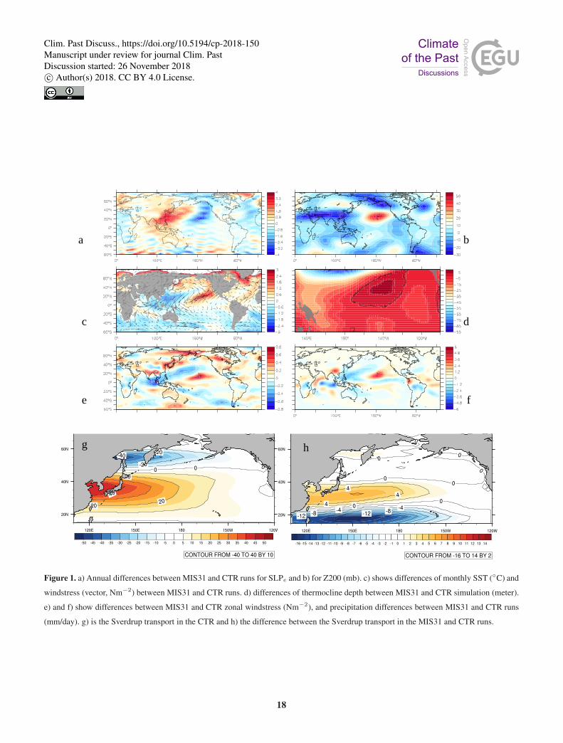
Figures 1a,b show the eddy SLP (SLP with the zonal mean removed, SLPe) and the Z200 (geopotential height at 200 hPa with30

the zonal mean removed). This strategy is important, because changes in circulation are dictated by changes to the gradient of

geopotential rather than absolute magnitude anomalies (He etal., 2018). At the surface, SLPe anomalies exhibit an increase in

the western North Pacific subtropical high in opposite to the drop in the eastern North Pacific (Fig 1a). This partially supports

previous results by Mantsis etal. (2013), who found a large strengthening and a northward and westward expansion of the

northern Pacific summer anticyclone, driven by changes in the timing of perihelion.35

According to Cook and Held (1988) and Timmermann etal. (2004) the meridional circulation v′ is proportional to the mean

westerly circulation u > 0, which is also modulated by the seasonal cycle of the SLP. In the upper troposphere (200 hPa), this

4


induces southward anomalies over the eastern Pacific and northward and low-pressure anomalies on the downstream side of the

Tibetan plateau in MIS31 (Fig. 1b); hence, weakening the jet stream in the MIS31 climate compared to the CTR counterpart.

This vertical structure with baroclinic anomalous pattern in particular over East Asia and western Pacific may be related to the5

ENSO dynamics in the MIS31 climate, as will be verified later.

These changes in the stationary wave induce substantial modifications in the windstress and SST/near surface air tempera-

tures features delivered by the MIS31 climate. Indeed, Fig. 1c depicts warmer SSTs in the northeast and subtropical Pacific but

cooler temperatures in the west Pacific. These changes along the equatorial belt are primary induced by weaker northeast trade

winds that reduced evaporative cooling and lead to less vigorous equatorial upwelling between 0-20◦N. Moreover, windstress10

changes in the eastern Pacific reduce the cold tongue strength (Figs. 1c,d).

The ICTP-CGCM properly reproduces the equatorial thermocline depth (using the depth of maximum vertical temperature

gradient) compared to the Levitus dataset (Levitus etal., 2000). The MIS31 forcing leads to a shallower thermocline and

reduction of its zonal gradient (Fig. 1d), which is primarily related to the anomalous wind flow (e.g., Zebiak and Cane,

1987; An etal., 1999). A deeper thermocline however, is observed in part of the NIÑO3 region (Fig. 1d, contour). In the15

eastern Pacific, thermocline dynamics have been associated with changes in SST, the air-sea coupling, and ENSO (Leduc etal.,

2009; Yang and Wang, 2009). This implies a weaker Walker circulation during the MIS31 interval that is supported by SST

reconstructions (from Ocean Drilling Program sites 849, 847, 846, and 871) in the western and eastern equatorial Pacific

(McClymont and Rosell-Melé, 2005).

Over the western Pacific, stronger equatorward winds (Figs. 1c,e) lead to cooler SSTs and enhanced subtropical cell, in con-20

cert with an intensified subtropical gyre (Figs. 1g,h). The wind-driven circulation may be evaluated by the Sverdrup transport

defined as:

ψ(x) =1βρ

x∫

xe

∂τx∂y

dx (1)

where β is the meridional derivative of the Coriolis parameter, ρ is the mean density of sea water, and τx is the zonal

component of the wind stress. The integral is computed from the eastern to the western boundary in the North Pacific using25

modeled atmospheric wind stress data. The ICTP-CGCM model simulates the Sverdrup transport quite well (Fig. 1g) compared

to the magnitude of the Sverdrup transport estimated from the International Comprehensive Ocean-Atmosphere Data Set

(ICOADS; Woodruff etal., 2011).

The intensification of the Sverdrup transport by up to 6 Sv between 20-40◦N in the Kuroshio region induces negative SST

anomalies due to the intrusion of colder sub-surface water related to the speed up of the subtropical cell (Fig. 1h). These30

processes are in phase with increased precipitation in the central Pacific region, but dryer conditions are noted in the Warm

Pool region (Fig 1f). The convergence of wind anomalies (Fig. 1c) also indicates westerly flow with potential implications for

the ENSO dynamics (Eisenman etal., 2005). In the Atlantic Ocean, warmer conditions are noticed in most of the NH which are

tightly related to orbitally driven wind anomalies. While the northern Pacific shows a baroclinic structure, the Atlantic shows a

barotropic pattern demonstrated by the SLPe and Z200 (Figs. 1a,b).

5


3 Harmonic analyses of MIS31 and CTR climates5

Additional evaluation on modifications of the annual and semi-annual oscillation are provided below through harmonic anal-

yses. The first order harmonics of meteorological parameters show long-term effects, while higher order harmonics represent

the effects of short-term fluctuations that characterize different climate regimes and transition regions. Using this mathematical

approach allows the identification of dominant climate features in the space–time domain desintangling small and large-scale

processes driven by distinct periodicity (Justino etal., 2010, 2016).10

Changes in the harmonic variance and amplitude are highly correlated with the amount of incoming shortwave radiation

(SSR) in the MIS31 climate, as shown by differences in the 1st harmonic (Fig. 2a-f) of SSR, SST, SLP and the HF. It has

long been recognized that the equatorial climate exhibits an annual component which strongly dominates SST, windstress, and

precipitation (Li and Philander, 1996, 1997). Nevertheless, the western equatorial Pacific and to a lesser extent the western At-

lantic temporal variability present largest variance in the semi-annual component (2nd harmonic). The semi-annual component15

is strongly influenced by ocean-atmosphere interactions, in which the surface atmospheric flow and SST, feedback on the cloud

structure further modifying the SSR and oceanic heat flux.

Figure 2a-d reveal that the semi-annual component, which is dominant in the western equatorial Pacific under current con-

ditions (not shown), is weaker in the MIS31 climate allowing larger variance in the annual harmonic. This is highlighted in

particular by SST and SLP distributions which potentially impact on ENSO characteristics (2b-d). It is also shown that similar20

patterns are displyed by the SSR and HF, and SST and SLP harmonics. The former (SSR and HF) experiences an interhemi-

spheric distribution whereas the latter i(SST and SLP) is dominated by an equatorial east-west dipole in the Pacific.

Figures 2e-h show changes in the amplitude of the 1st harmonic between the MIS31 and CTR simulations. The main features

are shown as larger (smaller) NH (SH) amplitudes deliverd by the MIS31 run, in particular along the continental margins and

in the Warm Pool/western Pacific area. Insofar as the western Pacific changes are concerned, it has been found that the local25

increase in windstress during (JJA) driven by the seasonality of SLP over central and western Pacific, are in concert with the

higher SSR, SST and HF amplitudes. These changes in seasonality dramatically alter the MIS31 climate compared to the CTR

climate in both spatial patterns and the main mode of variability (further discussed below).

This structure is not seen in the equatorial Atlantic where variance differences between the MIS31 and the CTR are merid-

ional. In fact, under CTR conditions this can be interpreted as the tropical Atlantic variability (TAV) related to the continental30

monsoon forcing, windstress and air-sea interaction (Deser etal., 2010). However, due to orbitally-driven changes in SSR (Fig.

2a), the MIS31 climate in the tropical Atlantic shows weakening of the annual component southward to 10◦N, and an intesifi-

cation of the semi-annual oscillation between 10-20◦N compared to the CTR run (Fig. 2b).

The SLP differences are more complex, showing a pattern that differs from zonal or meridional features (Fig. 2c), even

though they are correlated with SSTs in the western Pacific (Warm Pool region). In the Atlantic, the 1st harmonic weakens,

allowing for sub-seasonal temporal variability (lower order harmonics) enhanced nearby the African coast (Fig. 2c).

6


4 MIS31 - Temporal and spatial characteristics of ENSO

It is expected that those changes in the atmospheric zonal and meridional circulations and the wind-driven oceanic flow can5

result in modifying ENSO frequency and power. The following explores the influence of the MIS31 forcing on ENSO indices.

Among several mechanisms related to ENSO dynamics, the magnitude of the seasonal cycle in the equatorial region charac-

terizes its onset, intensity, and frequency (Liu, 2002a; Nonaka etal., 2002; Timmermann etal., 2007). It has been argued that in

case of strong seasonal cycle, the ENSO signal can be locked in phase and frequency with this external forcing, thus reducing

its magnitude. The ENSO signal may also differ in strength and influence if computed over distinct oceanic regions, such as10

those defined by NIÑO3, NIÑO34 or NIÑO4 (Wilson etal., 2014, 2016).

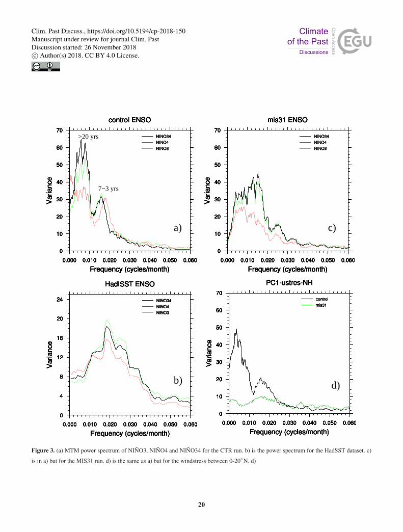
Figures 3a,b show the ENSO power spectrum computed for the NIÑO34, NIÑO3, and the NIÑO4 using the Hadley Centre

Sea Surface Temperature data set (HadISST; Rayner etal., 2003) and the CTR simulation. This is achieved by applying the

Multi-Taper method (MTM; Thomson, 1982) a technique that has been demonstrated to fill limitations of conventional Fourier

analysis.15

All periodicities mentioned below are significant at the 95% confidence level. Compared with the power spectrum delivered

by the HadISST, the ICTP-CGCM shows sharper peak in the 3-7 year band for all NIÑO indices (Fig 3a). The HadISST spec-

trum shows maximum concentration of power spanning the 3-5 year period. Under CTR conditions, significant concentration

of power is also dominant on the multidecadal time scale between 15-30 years. Similar periodicity has been previously found

by Nonaka etal. (2002). (Nonaka etal., 2002) attributes the equatorial decadal variability to the influence of winds in the trade20

wind bands which modifies the strength of the sub-tropical cell. It is interesting to note that NIÑO34, NIÑO3, and NIÑO4

differ in reproducing the decadal frequency, weakest in the NIÑO4. The HadISST does not show any periodicity on decadal

time scales; even though the SST data spans 1870 to 2016, the length of the timeseries does not seem to capture this lower

frequency. It has to be mentioned that Rodgers etal. (2004) claims that the zonal asymmetry related to decadal variability in

the HadISST observations is weaker and not as regular as for instance in the ECHO-G model.25

The weakening of decadal variability in the NIÑO4 region may be related to wind variability in the off-equatorial tropics as

proposed by Nonaka etal. (2002). This assumption has been verified by computing the correlation pattern associated with the

NIÑO indices. It turns out that the NIÑO4 relationship with the zonal windstress within 10-30◦N is considerably weaker than

that of NIÑO34 or NIÑO3 (not shown). Moreover, this weaker correlation between the NIÑO4 and windstress is not confined

to the equatorial region but extends to the extratropics.30

The incorporation of MIS31 boundary conditions drastically modifies the temporal variability of the interglacial ENSO (Fig.

3c). This simulation shows stronger power spectrum at interannual time scales between 3-7 years. Evaluation of the main

causes related to the strengthening of the interannual variability in the MIS31 climate compared with the CTR counterpart

is not straitforward. It has been found that an increased meridional gradient of SST and wind stress in the NH tropics (Fig.

2a), as simulated by the MIS31 run, may lead to stronger interannual equatorial variability in the MIS31 climate (Liu, 2002a,

b; Erb etal., 2015). Likewise, the weaker seasonal cycle of the windstress in the MIS31 simulation may lead to stronger

ENSO power at 3-7 years (Chang etal., 1994). The CTR climate SOI power spectrum also shows enhanced power at similar

7


frequencies found for the NIÑO34 and the NIÑO3 indices. This is in line with the spectrum of equatorial winds (0-20◦N) that

shows enhanced power also at interdecadal time scales (Fig 3d).5

The opposite is delivered by the MIS31 simulation, a fact that usefully serves to support the assumption of weaker decadal

air-sea interaction during this interglacial. Indeed, for the MIS31 simulation, correlation values between the NIÑO34 index

and the 1st principal component (PC1) of windstress computed at 0-20◦N are very low; whereas for the CTR run, these

values are 0.6 when all timescales are included and 0.4 for conditions in which frequencies below 10 years have been filtered

out. Though previous studies have claimed that the equatorial Pacific interannual variability is primary forced by equatorial10

windstress (Nonaka etal., 2002; Timmermann and Jin, 2002), and the decadal variability is strongly connected to the off-

equatorial windstress, our results show that the atmospheric flow between 0-20◦N can induce decadal variability.

In fact, the decadal variability found in the CTR NIÑO34 power spectrum fits nicely with the proposed mechanism raised

by Farneti etal. (2014). The SST anomalies at the equator induce changes in the windstress curl over the western Pacific, that

generate SST anomalies fluctuating on decadal time scales through tropical-subtropical interactions. Individual analyses to15

verify the roles of the North and South Pacific in inducing the decadal variability, demonstrate that most changes of power

can be explained by the NH contribution. Interestingly, the NIÑO34 and windstress anomalies between 20◦S-0 are highly

anti-correlated with values of about 0.6 in both simulations. However, only in the MIS31 climate the windstress spectrum does

exhibit enhanced interannual variability, indicating that the MIS31 ENSO dynamics are also driven at the 3-7 year period by

the SH flow. A fact that is not seen for the CTR climate.20

Turning to the regression patterns induced by the NIÑO34 indices, Figure 4 shows that our coupled model reproduces the

main tropical SST response to NIÑO34 (Fig. 4a), compared for instance with Cai etal. (2015). The patterns are displayed as

amplitudes by regressing hemispheric anomalies on the standardized first principal component time series. The intensification

of the NIÑO34 signal does not project substantial change in SST, though in the western Pacific, anomalies between ± 0.3◦C

are noted (Fig. 4b).25

The impact of NIÑO34 on SLP (Fig. 4c) extends globally and is fairly reproduced by the ICTP-CGCM compared to the

National Centers for Environmental Precition - National Center for Atmospheric Research (NCEP-NCAR) reanalysis (Ji etal.,

2015). The zonal dipole results from the contribution of the baroclinic component over the eastern Pacific and barotropic

component over western Pacific, both related to the SST anomalies (Figs. 4c, a). The MIS31 NIÑO34 weakens the barotropic

and baroclinic patterns of the SLP as shown by the differences in the MIS31-CTR regression (Figs. 4c,d). In the equatorial30

region, the anomalies are related to the intensified winds nearby the Warm Pool region but weakening mid-latitude westerlies

in both the northern Pacific and Atlantic (Figs. 4e,f). In the following, we compare temperature differences between the MIS31

and CTR to compiled data by Wet etal. (2016), but with focus on the ENSO responses (Table 2).

This is achieved by comparing the modeled SST anomalies for JJA to SSTs differences between the MIS31 and CTR

delivered by the regression pattern related to the NIÑO34 index (∆T). Differences between the reconstructions and the NOAA

Extended Reconstructed SST V3b/ERA-I are also shown (∆Tre). Overall, model results and reconstructions agree indicating

that the ENSO works in line with the astronomical forcing, inducing warming (√

in Table 2) however in some cases it acts in

the opposite (X in Table 2).5

8


4.1 Global and monsoonal precipitation

As shown in Figure 1f), it is evident that most wet and dry conditions in the MIS31 compared to the CTR are in agreement

with the anomalous temperature pattern and diabatic heating, in line with ENSO-related precipitation (Dai and Arkin, 2017).

Exception is found over southern Asia that experiences more precipitation despite the drop in temperatures, which may indicate

the contribution of extratropical large-scale atmospheric dynamics.10

To further investigate the MIS31 climate features it is evaluated the correlation between precipitation computed over re-

gional Asia monsoonal domains, as defined by Yim etal. (2014) and the NINO34 index. The domains are: the Asia monsoon

(AM, 10◦N-45◦N, 70◦E-150◦E); Australia monsoon (AUS, 5◦S-20◦S, 110◦E-150◦E); East Asia monsoon (EA, 22.5◦S-45◦N,

110◦E-135◦E); western north Pacific monsoon (WNP, 12.5◦N-22.5◦N, 110◦E-135◦E) and Indian monsoon (IN, 10◦N-30◦N,

70◦E-105◦E).15

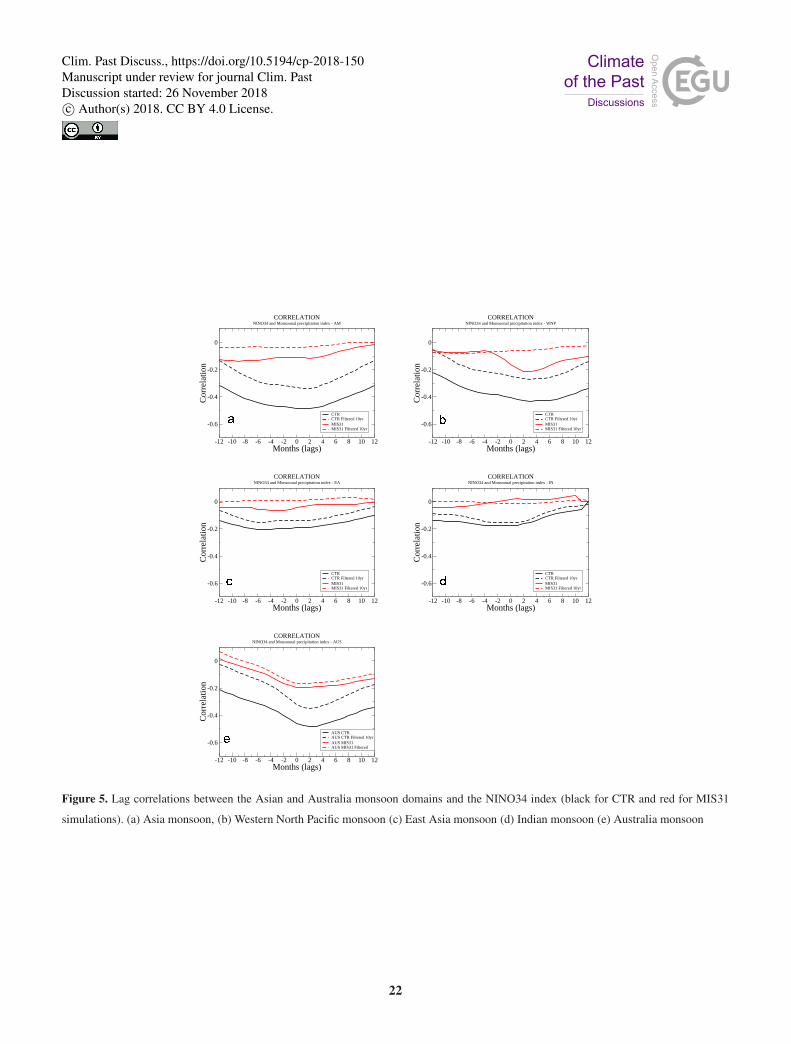
Estimates of changes in precipitation for past interglacials are still scarce, but our MIS31 simulation agrees with other studies

showing enhanced Asia summer monsoon (Fig. 5a), during interglacials (An, 2000; Sun etal., 2010a). Enhanced seasonality

and greater annual values of precipitation have also been documented across the East Russian Arctic in line with our modeling

experiment (Melles etal., 2012). This is also true for the Asian monsoon insofar as seasonality is concerned (Fig. 5a). Contro-

versy is raised by Oliveira etal. (2017) who argue that reduced seasonality in precipitation along western Mediterranean region20

during MIS31 leads to forest decline. Reduced seasonality during the MIS31 in that region is not supported by our MIS31

climate simulation, which in fact shows an increase in both summer and fall/winter precipitation (not shown).

Turning in particular for the monsoonal domains, it is clear the weakening of the relationship between the NINO34 and

the Asia and Australia monsoonal domains during the MIS31 as compared to the CTR counterparts (Fig. 5). It should be

mentioned that the equatorial Pacific seems to have a direct influence on the AM, WNP and the AUS monsoon precipitation25

(Fig. 5a,b,e). This is not the case for the East Asia and Indian monsoon. Under current conditions, the NINO34 is negatively

correlated with monsoonal indices with values by up to -0.5 for the AM and AUS, in which the NINO34 leads by 2 months (Fig.

5a,e). Interestingly, despite stronger interannual ENSO in the MIS31 climate the correlation between the SST and precipitation

indices is extremely reduced for AM, AUS and WNP monsoons during the interglacial period (Fig. 5e).

In order to verify the impact of decadal variability on the link between the NINO34 and the monsoon, Figure 5 also show30

the correlation between the indices but filtering out the interannual periodicity. This reveals that the decadal variability is

responsable for about 40% of the correlation in the CTR climate. As should be expected, by removing the interannual frequency

in the MIS31 climate, correlations values turn very small which indicate that changes in AUS, WNP and AM precipitation for

this interglacial are more closely connected to hemispherical features than to the tropical-extratropical climate interaction.

5 Concluding Remarks

This investigation centered on a comparison between present-day conditions (CTR) and those characteristic of a super-5

interglacial epoch, the Marine Isotope Stage 31 (MIS31). Using coupled global climate model simulations (ICTP-CGCM),

we have first demonstrated significant changes in the spatial patterns and seasonality of sea-level pressure, sea-surface tem-

9


peratures, and heat fluxes during the MIS31 climate compared to present-day conditions, and these changes have a significant

impact on the main modes of variability. Anomalous equatorial windstress associated with a modified seasonal cycle in the

MIS31 simulation leads to stronger ENSO variability compared to the present-day climate. Moreover, the decadal variability

differs dramatically in the MIS31 simulation from that characteristic of present-day conditions. This decadal variability also

differs greatly across the ENSO diversity spectrum, with off-equatorial atmospheric circulation playing a significant role in

inducing decadal variability.5

Evaluation between paleoreconstruction and modeling results is a complex task, because reconstructions depict dominant

signals in a particular time interval and locale. Thus, they cannot be assumed to geographically represent large-scale domains,

and their ability to reproduce long-term environmental conditions should be considered with care.

Discrepancies between modeling results and paleoreconstructions for the MIS31 climate, which occurred under very par-

ticular conditions and high seasonality, may unfortunately be expected. The MIS31 may have been dominated for instance10

by vegetation patterns drastically different than today. This modifies the global evapotranspiration rates and the hydrological

cycle, producing precipitation that can differ greatly from model results. This suggests that uncertainties in the model may be

reduced when including more realistic boundary conditions that currently are not available.

10


References

An, S., Jin, F., and Kang, I.: The Role of Zonal Advection Feedback in Phase Transition and Growth of ENSO in the Zebiak-Cane Model, J.15

Meteorol. Soc. Japan, 1999.

An, S., Timmermann, A., Bejarano, L., Jin, F. F., Justino, F., Liu, Z., and Tudhope, A. W.: Modeling Evidence For Enhanced El Nino-Southern

Oscillation Amplitude During The Last Glacial Maximum, Paleoceanography, 19, doi:10.1029/2004PA001102, 2004.

An, Z.: The history and variability of the East Asian paleomonsoon climate, Quaternary Science Reviews, 19, 171 – 187,

https://doi.org/https://doi.org/10.1016/S0277-3791(99)00060-8, http://www.sciencedirect.com/science/article/pii/S0277379199000608,20

2000.

Bjerknes, J.: Atlantic air-sea interaction, Advances in Geophysics, 10, 1–82, 1964.

Cai, W., Borlace, S., Lengaigne, M., Van Rensch, P., Collins, M., Vecchi, G., Timmermann, A., Santoso, A., McPhaden, M. J.,

Wu, L., et al.: Increasing frequency of extreme El Niño events due to greenhouse warming, Nature Climate Change, 4, 111–116,

https://doi.org/10.1038/nclimate2100, 2014.25

Cai, W., Santoso, A., Wang, G., Yeh, S.-W., An, S.-I., Cobb, K. M., Collins, M., Guilyardi, E., Jin, F.-F., Kug, J.-S., et al.: ENSO and

greenhouse warming, Nature Climate Change, 5, 849, 2015.

Chang, P., Wang, B., Li, T., and Ji, L.: Interactions between the seasonal cycle and the Southern Oscillation - Frequency entrainment

and chaos in a coupled ocean-atmosphere model, Geophysical Research Letters, 21, 2817–2820, https://doi.org/10.1029/94GL02759,

http://dx.doi.org/10.1029/94GL02759, 1994.30

Coletti, A. J., DeConto, R. M., Brigham-Grette, J., and Melles, M.: A GCM comparison of Plio-Pleistocene interglacial-glacial periods in re-

lation to Lake El’gygytgyn, NE Arctic Russia, Climate of the Past Discussions, 10, 3127–3161, https://doi.org/10.5194/cpd-10-3127-2014,

http://www.clim-past-discuss.net/10/3127/2014/, 2014.

Cook, K. and Held, I.: Stationary Waves of the Ice Age Climate, J. Clim., 1, 807–819,

https://doi.org/doi.org/10.1175/1520-0442(1988)001<0807:SWOTIA>2.0.CO;2, 1988.35

Crundwell, M., Scott, G., Naish, T., and Carter, L.: Glacial–interglacial ocean climate variability from planktonic foraminifera during the

Mid-Pleistocene transition in the temperate Southwest Pacific, ODP Site 1123, Palaeogeography, Palaeoclimatology, Palaeoecology, 260,

202–229, 2008.

Dai, N. and Arkin, P. A.: Twentieth century ENSO-related precipitation mean states in twentieth century reanalysis, reconstructed precipita-

tion and CMIP5 models, Climate dynamics, 48, 3061–3083, 2017.

Dee, D. P., Uppala, S. M., Simmons, A., Berrisford, P., Poli, P., Kobayashi, S., Andrae, U., Balmaseda, M., Balsamo, G., Bauer, d. P., et al.:5

The ERA-Interim reanalysis: Configuration and performance of the data assimilation system, Quarterly Journal of the royal meteorological

society, 137, 553–597, 2011.

Deser, C., Alexander, M. A., Xie, S.-P., and Phillips, A. S.: Sea Surface Temperature Variability: Patterns and Mechanisms, Annual Review

of Marine Science, 2, 115–143, https://doi.org/10.1146/annurev-marine-120408-151453, 2010.

Dolan, A. M., Hunter, S. J., Hill, D. J., Haywood, A. M., Koenig, S. J., Otto-Bliesner, B. L., Abe-Ouchi, A., Bragg, F., Chan, W.-L., Chandler,10

M. A., Contoux, C., Jost, A., Kamae, Y., Lohmann, G., Lunt, D. J., Ramstein, G., Rosenbloom, N. A., Sohl, L., Stepanek, C., Ueda, H.,

Yan, Q., and Zhang, Z.: Using results from the PlioMIP ensemble to investigate the Greenland Ice Sheet during the mid-Pliocene Warm

Period, Climate of the Past, 11, 403–424, https://doi.org/10.5194/cp-11-403-2015, http://www.clim-past.net/11/403/2015/, 2015.

11


Dyez, K. A. and Ravelo, A. C.: Dynamical changes in the tropical Pacific warm pool and zonal SST gradient during the Pleis-

tocene, Geophysical Research Letters, 41, 7626–7633, https://doi.org/10.1002/2014GL061639, http://dx.doi.org/10.1002/2014GL061639,15

2014GL061639, 2014.

Eisenman, I., Yu, L., and Tziperman, E.: Westerly wind bursts: ENSO’s tail rather than the dog?, Journal of Climate, 18, 5224–5238,

https://doi.org/10.1175/JCLI3588.1, 2005.

Erb, M., Broccoli, A., Graham, N., Clement, A., Wittenberg, A., and Vecchi, G.: Response of the equatorial pacific seasonal cycle to orbital

forcing, Journal of Climate, 28, 9258–9276, https://doi.org/10.1175/JCLI-D-15-0242.1, 2015.20

Farneti, R., Molteni, F., and Kucharski, F.: Pacific interdecadal variability driven by tropical-extratropical interactions, Climate Dynamics,

42, 3337–3355, https://doi.org/10.1007/s00382-013-1906-6, 2014.

Frei, A. and Gong, G.: Decadal to century scale trends in North American snow extent in coupled atmosphere-ocean general circulation

models, Geophysical Research Letters, 32, n/a–n/a, https://doi.org/10.1029/2005GL023394, http://dx.doi.org/10.1029/2005GL023394,

l18502, 2005.25

He, C., Lin, A., Gu, D., Li, C., Zheng, B., Wu, B., and Zhou, T.: Using eddy geopotential height to measure the western North Pacific

subtropical high in a warming climate, Theoretical and Applied Climatology, pp. 681–691, https://doi.org/10.1007/s00704-016-2001-9,

2018.

Herbert, T. D., Peterson, L. C., Lawrence, K. T., and Liu, Z.: Tropical ocean temperatures over the past 3.5 million years, Science, 328,

1530–1534, 2010a.30


1530–1534, 2010b.


1530–1534, 2010c.

Honisch, B., Hemming, N. G., Archer, D., Siddall, M., and McManus, J. F.: Atmospheric Carbon Dioxide Con-35

centration Across the Mid-Pleistocene Transition, Science, 324, 1551–1554, https://doi.org/10.1126/science.1171477,

http://www.sciencemag.org/content/324/5934/1551.abstract, 2009.

Ji, X., Neelin, J. D., and Mechoso, C. R.: El Nino-Southern Oscillation Sea Level Pressure Anomalies in the Western Pacific: Why Are They

There?, Journal of Climate, 28, 8860–8872, https://doi.org/10.1175/JCLI-D-14-00716.1, 2015.

Jost, A., Lunt, D., Kageyama, M., Abe-Ouchi, A., Peyron, O., Valdes, P., and Ramstein, G.: High-resolution simulations of the Last Glacial

Maximum climate over Europe: a solution to discrepancies with continental palaeoclimatic reconstructions?, Clim. Dyn., 24, 557–590,

2005.

Justino, F., Setzer, A., Bracegirdle, T. J., Mendes, D., Grimm, A., Dechiche, G., and Schaefer, C. E. G. R.: Harmonic analysis of climatological5

temperature over Antarctica: present day and greenhouse warming perspectives, Internation Journal of Climatology, doi: 10.1002/joc.2090,

2010.

Justino, F., Stordal, F., Vizy, E. K., Cook, K. H., and Pereira, M. P. S.: Greenhouse Gas Induced Changes in the Seasonal

Cycle of the Amazon Basin in Coupled Climate-Vegetation Regional Model, Climate, 4, https://doi.org/10.3390/cli4010003,

http://www.mdpi.com/2225-1154/4/1/3, 2016.10

Justino, F., Lindemann, D., Kucharski, F., Wilson, A., Bromwich, D., and Stordal, F.: Oceanic response to changes in the WAIS and as-

tronomical forcing during the MIS31 superinterglacial, Climate of the Past, 13, 1081–1095, https://doi.org/10.5194/cp-13-1081-2017,

https://www.clim-past.net/13/1081/2017/, 2017.

12


Karami, M., Herold, N., Berger, A., Yin, Q., and Muri, H.: State of the tropical Pacific Ocean and its enhanced impact on precipitation over

East Asia during Marine Isotopic Stage 13, Climate dynamics, 44, 807–825, 2015.15

Karamperidou, C., Di Nezio, P. N., Timmermann, A., Jin, F.-F., and Cobb, K. M.: The response of ENSO flavors to mid-

Holocene climate: Implications for proxy interpretation, Paleoceanography, 30, 527–547, https://doi.org/10.1002/2014PA002742,

http://dx.doi.org/10.1002/2014PA002742, 2014PA002742, 2015.

Kucharski, F., Molteni, F., and Bracco, A.: Decadal interactions between the western tropical Pacific and the North Atlantic Oscillation,

Clim. Dyn., 26, 79–91, 2006.20

Kucharski, F., Ikram, F., Molteni, F., Farneti, R., Kang, I.-S., No, H.-H., King, M. P., Giuliani, G., and Mogensen, K.:

Atlantic forcing of Pacific decadal variability, Climate Dynamics, 46, 2337–2351, https://doi.org/10.1007/s00382-015-2705-z,

http://dx.doi.org/10.1007/s00382-015-2705-z, 2016.

Lawrence, K. T., Herbert, T. D., Brown, C. M., Raymo, M. E., and Haywood, A. M.: High-amplitude variations in North Atlantic sea

surface temperature during the early Pliocene warm period, Paleoceanography, 24, n/a–n/a, https://doi.org/10.1029/2008PA001669,25

http://dx.doi.org/10.1029/2008PA001669, pA2218, 2009.

Leduc, G., Vidal, L., Cartapanis, O., and Bard, E.: Modes of eastern equatorial Pacific thermocline variability: Implica-

tions for ENSO dynamics over the last glacial period, Paleoceanography, 24, n/a–n/a, https://doi.org/10.1029/2008PA001701,

http://dx.doi.org/10.1029/2008PA001701, 2009.

Levitus, S., Antonov, J. I., Boyer, T. P., and Stephens, C.: Warming of the World Ocean, Science, 287, 2225–2229,30

https://doi.org/10.1126/science.287.5461.2225, http://science.sciencemag.org/content/287/5461/2225, 2000.

Li, L., Li, Q., Tian, J., Wang, P., Wang, H., and Liu, Z.: A 4-Ma record of thermal evolution in the tropical western Pacific and its implications

on climate change, Earth and Planetary Science Letters, 309, 10–20, https://doi.org/10.1016/j.epsl.2011.04.016, 2011.

Li, T. and Philander, S.: On the seasonal cycle of the equatorial Atlantic Ocean, Journal of climate, 10, 813–817, 1997.

Li, T. and Philander, S. G. H.: On the Annual Cycle of the Equatorial Eastern Pacific, J. Clim., 9, 2986–2998, 1996.35

Lisiecki, L. E. and Raymo, M. E.: A Pliocene-Pleistocene stack of 57 globally distributed benthic δ 18O records, Paleoceanography, 20,

n/a–n/a, https://doi.org/10.1029/2004PA001071, http://dx.doi.org/10.1029/2004PA001071, pA1003, 2005.

Liu, Z.: A simple model study of the forced response of ENSO to an external periodic forcing., J. Clim., 15, 1088–1098,

https://doi.org/10.1175/1520-0442(2002)015<1088:ASMSOE>2.0.CO;2, 2002a.

Liu, Z.: A Simple Model Study of ENSO Suppression by External Periodic Forcing*, Journal of climate, 15, 1088–1098,

https://doi.org/10.1175/1520-0442(2002)015<1088:ASMSOE>2.0.CO;2, 2002b.

Madec, G.: NEMO: the OPA ocean engine, Note du Pole de Modelisation, pp. 1–110, Note du Pôle de modélisation de l’Institut Pierre-Simon

Laplace No 27, http://dx.doi.org/10.1029/137GM07, 2008.5

Mantsis, D. F., Clement, A. C., Kirtman, B., Broccoli, A. J., and Erb, M. P.: Precessional Cycles and Their Influence on the North Pacific and

North Atlantic Summer Anticyclones, Journal of Climate, 26, 4596–4611, https://doi.org/10.1175/JCLI-D-12-00343.1, 2013.

Mantua, N. J., Hare, S. R., Zhang, Y., Wallace, J. M., and Francis, R. C.: A Pacific interdecadal climate oscillation with impacts on salmon

production, Bulletin of the american Meteorological Society, 78, 1069–1079, 1997.

Martínez-Garcia, A., Rosell-Melé, A., McClymont, E. L., Gersonde, R., and Haug, G. H.: Subpolar link to the emergence of the modern10

equatorial Pacific cold tongue, Science, 328, 1550–1553, https://doi.org/10.1126/science.1184480, 2010.

McClymont, E. L. and Rosell-Melé, A.: Links between the onset of modern Walker circulation and the mid-Pleistocene climate transition,

Geology, 33, 389–392, 2005.

13


McClymont, E. L., Rosell-Melé, A., Giraudeau, J., Pierre, C., and Lloyd, J. M.: Alkenone and coccolith records of the mid-Pleistocene

in the south-east Atlantic: implications for the index and South African climate, Quaternary Science Reviews, 24, 1559–1572,15

https://doi.org/10.1016/j.quascirev.2004.06.024, 2005.

Medina-Elizalde, M., Lea, D. W., and Fantle, M. S.: Implications of seawater Mg/Ca variability for Plio-Pleistocene tropical climate recon-

struction, Earth and Planetary Science Letters, 269, 585–595, https://doi.org/10.1016/j.epsl.2008.03.014, 2008.

Melles, M., Brigham-Grette, J., Minyuk, P. S., Nowaczyk, N. R., Wennrich, V., DeConto, R. M., Anderson, P. M., Andreev, A. A., Co-

letti, A., Cook, T. L., Haltia-Hovi, E., Kukkonen, M., Lozhkin, A. V., Ros P., Tarasov, P., Vogel, H., and Wagner, B.: 2.8 Million20

Years of Arctic Climate Change from Lake El-gygytgyn, NE Russia, Science, 337, 315–320, https://doi.org/10.1126/science.1222135,

http://www.sciencemag.org/content/337/6092/315.abstract, 2012.

Morice, C. P., Kennedy, J. J., Rayner, N. A., and Jones, P. D.: Quantifying uncertainties in global and regional temperature change us-

ing an ensemble of observational estimates: The HadCRUT4 data set, Journal of Geophysical Research: Atmospheres, 117, n/a–n/a,

https://doi.org/10.1029/2011JD017187, http://dx.doi.org/10.1029/2011JD017187, d08101, 2012.25

Naafs, B. D. A., Hefter, J., Gruetzner, J., and Stein, R.: Warming of surface waters in the mid-latitude North Atlantic during Heinrich events,

Paleoceanography, 28, 153–163, https://doi.org/10.1029/2012PA002354, http://dx.doi.org/10.1029/2012PA002354, 2013.

Naish, T., Powell, R., Levy, R., Wilson, G., Scherer, R., Talarico, F., Krissek, L., Niessen, F., Pompilio, M., Wilson, T., Carter, L., DeConto,

R., Huybers, P., McKay, R., Pollard, D., Ross, J., Winter, D., Barrett, P., Browne, G., Cody, R., Cowan, E., Crampton, J., Dunbar, G.,

Dunbar, N., Florindo, F., Gebhardt, C., Graham, I., Hannah, M., Hansaraj, D., Harwood, D., Helling, D., Henrys, S., Hinnov, L., Kuhn, G.,30

Kyle, P., Lufer, A., Maffioli, P., Magens, D., Mandernack, K., McIntosh, W., Millan, C., Morin, R., Ohneiser, C., Paulsen, T., Persico, D.,

Raine, I., Reed, J., Riesselman, C., Sagnotti, L., Schmitt, D., Sjunneskog, C., Strong, P., Taviani, M., Vogel, S., Wilch, T., and Williams,

T.: Obliquity-paced Pliocene West Antarctic ice sheet oscillations, Nature, 458, 322–328, 2009.

Nicolas, J. P., Vogelmann, A. M., Scott, R. C., Wilson, A. B., Cadeddu, M. P., Bromwich, D. H., Verlinde, J., Lubin, D., Russell, L. M.,

Jenkinson, C., et al.: January 2016 extensive summer melt in West Antarctica favoured by strong El Niño., Nature communications, 8,35

15 799, 2017.

Nonaka, M., Xie, S.-P., and McCreary, J. P.: Decadal variations in the subtropical cells and equatorial pacific SST, Geophysical Research

Letters, 29, 20–1–20–4, https://doi.org/10.1029/2001GL013717, http://dx.doi.org/10.1029/2001GL013717, 2002.

Oliveira, D., Go?i, M. F. S., Naughton, F., Polanco-Mart?nez, J., Jimenez-Espejo, F. J., Grimalt, J. O., Martrat, B., Voelker, A. H., Trigo, R.,

Hodell, D., Abrantes, F., and Desprat, S.: Unexpected weak seasonal climate in the western Mediterranean region during MIS 31, a high-

insolation forced interglacial, Quaternary Science Reviews, 161, 1 – 17, https://doi.org/https://doi.org/10.1016/j.quascirev.2017.02.013,5

http://www.sciencedirect.com/science/article/pii/S0277379116306515, 2017.

Peltier, W. and Solheim, L.: The climate of the Earth at Last Glacial Maximum: statistical equilibrium state and a mode of internal variability,

Quaternary Science Reviews, pp. 335–357, 2004.

Pollard, D. and DeConto, R.: Modelling West Antarctic ice sheet growth and collapse through the past five million years, Nature,

http://dx.doi.org/10.1038/nature07809, 2009.10

Rachmayani, R., Prange, M., and Schulz, M.: Intra-interglacial climate variability: model simulations of Marine Isotope Stages 1, 5, 11, 13,

and 15, Climate of the Past, 12, 677–695, https://doi.org/10.5194/cp-12-677-2016, https://www.clim-past.net/12/677/2016/, 2016.

Raymo, M., Grant, B., Horowitz, M., and Rau, G.: Mid-Pliocene warmth: stronger greenhouse and stronger conveyor, Marine Micropaleon-

tology, 27, 313–326, 1996.

14


Rayner, N. A., Parker, D. E., Horton, E. B., Folland, C. K., Alexander, L. V., Rowell, D. P., Kent, E. C., and Kaplan, A.: Global analyses15

of sea surface temperature, sea ice, and night marine air temperature since the late nineteenth century, Journal of Geophysical Research:

Atmospheres, 108, n/a–n/a, https://doi.org/10.1029/2002JD002670, http://dx.doi.org/10.1029/2002JD002670, 4407, 2003.

Rodgers, K. B., Friederichs, P., and Latif, M.: Tropical Pacific decadal variability and its relation to decadal modulations of ENSO, Journal

of Climate, 17, 3761–3774, 2004.

Russon, T., Elliot, M., Sadekov, A., Cabioch, G., Corrège, T., and De Deckker, P.: The mid-Pleistocene transition in the subtropical southwest20

Pacific, Paleoceanography, 26, n/a–n/a, https://doi.org/10.1029/2010PA002019, http://dx.doi.org/10.1029/2010PA002019, pA1211, 2011.

Scherer, R. P., Bohaty, S. M., Dunbar, R. B., Esper, O., Flores, J.-A., Gersonde, R., Harwood, D. M., Roberts, A. P., and Taviani, M.: Antarctic

records of precession-paced insolation-driven warming during early Pleistocene Marine Isotope Stage 31, Geophysical Research Letters,

35, https://doi.org/10.1029/2007GL032254, http://dx.doi.org/10.1029/2007GL032254, 2008.

Steig, E. J., Ding, Q., White, J. W., Küttel, M., Rupper, S. B., Neumann, T. A., Neff, P. D., Gallant, A. J., Mayewski, P. A., Taylor, K. C.,25

et al.: Recent climate and ice-sheet changes in West Antarctica compared with the past 2,000 years, Nature Geoscience, 6, 372–375,

https://doi.org/10.1038/ngeo1778, 2013.

Stocker, T. F., Dahe, Q., and Plattner, G.-K.: Climate Change 2013: The Physical Science Basis, Working Group I Contribution to the Fifth

Assessment Report of the Intergovernmental Panel on Climate Change. Summary for Policymakers (IPCC, 2013), 2013.

Sun, Y., An, Z., Clemens, S. C., Bloemendal, J., and Vandenberghe, J.: Seven million years of wind and precipitation variability on the30

Chinese Loess Plateau, Earth and Planetary Science Letters, 297, 525 – 535, https://doi.org/https://doi.org/10.1016/j.epsl.2010.07.004,

http://www.sciencedirect.com/science/article/pii/S0012821X10004425, 2010a.

Sun, Y., An, Z., Clemens, S. C., Bloemendal, J., and Vandenberghe, J.: Seven million years of wind and precipitation variability on the

Chinese Loess Plateau, Earth and Planetary Science Letters, 297, 525–535, 2010b.

Thompson, D. W. J. and Wallace, J. M.: Regional Climate Impacts of the Northern Hemisphere Annular Mode, Science, 293, 85–89, 2001.35

Thomson, D. J.: Spectrum estimation and harmonic analysis, Proc. IEEE, 70, 1055–1094, 1982.

Timmermann, A. and Jin, F.-F.: A Nonlinear Mechanism for Decadal El Niño Amplitude Changes, Geophysical Research Letters, 29, 3–1–

3–4, https://doi.org/10.1029/2001GL013369, http://dx.doi.org/10.1029/2001GL013369, 2002.

Timmermann, A., Justino, F., Jin, F.-F., and Goosse, H.: Surface temperature control in the North and tropical Pacific during the last glacial

maximum, Clim. Dyn., 23, 353–370, 2004.

Timmermann, A., Lorenz, S., An, S., Clement, A., and Xie, S.: The effect of orbital forcing on the mean climate and variability of the tropical

Pacific, Journal of Climate, 20, 4147–4159, https://doi.org/10.1175/JCLI4240.1, 2007.

Toniazzo, T.: Properties of El Nino–Southern Oscillation in different equilibrium climates with HadCM3, Journal of climate, 19, 4854–4876,5

https://doi.org/10.1175/JCLI3853.1, 2006.

Tudhope, A. W., Chilcott, C. P., McCulloch, M. T., Cook, E. R., Chappell, J., Ellam, R. M., Lea, D. W., Lough, J. M., and Shimmield, G. B.:

Variability in the El Niño-Southern Oscillation through a glacial-interglacial cycle, Science, 291, 1511–1517, 2001.

Valcke, S.: The OASIS3 coupler: a European climate modelling community software, Geoscientific Model Development, 6, 373–388,

https://doi.org/10.5194/gmd-6-373-2013, http://www.geosci-model-dev.net/6/373/2013/, 2013.10

Voelker, A. H., Salgueiro, E., Rodrigues, T., Jimenez-Espejo, F. J., Bahr, A., Alberto, A., Loureiro, I., Padilha, M., Rebo-

tim, A., and Rhl, U.: Mediterranean Outflow and surface water variability off southern Portugal during the early Pleis-

tocene: A snapshot at Marine Isotope Stages 29 to 34 (10201135 ka) , Global and Planetary Change, 133, 223 – 237,

https://doi.org/http://dx.doi.org/10.1016/j.gloplacha.2015.08.015, 2015.

15


Wet, G., Castañeda, I. S., DeConto, R. M., and Brigham-Grette, J.: A high-resolution mid-Pleistocene temperature record from Arctic Lake15

El’gygytgyn: a 50 kyr super interglacial from MIS 33 to MIS 31, Earth and Planetary Science Letters, 436, 56–63, 2016.

Wilson, A. B., Bromwich, D. H., Hines, K. M., and Wang, S.-h.: El Niño Flavors and Their Simulated Impacts on Atmospheric Circulation

in the High Southern Latitudes*, Journal of Climate, 27, 8934–8955, 2014.

Wilson, A. B., Bromwich, D. H., and Hines, K. M.: Simulating the mutual forcing of anomalous high-southern latitude atmospheric circula-

tion by El Niño flavors and the Southern Annular Mode, Journal of Climate, 2016.20

Woodruff, S. D., Worley, S. J., Lubker, S. J., Ji, Z., Eric Freeman, J., Berry, D. I., Brohan, P., Kent, E. C., Reynolds, R. W., Smith, S. R., and

Wilkinson, C.: ICOADS Release 2.5: extensions and enhancements to the surface marine meteorological archive, International Journal of

Climatology, 31, 951–967, https://doi.org/10.1002/joc.2103, http://dx.doi.org/10.1002/joc.2103, 2011.

Yang, H. and Wang, F.: Revisiting the thermocline depth in the equatorial Pacific*, Journal of Climate, 22, 3856–3863, 2009.

Yim, S.-Y., Wang, B., Liu, J., and Wu, Z.: A comparison of regional monsoon variability using monsoon indices, Climate dynamics, 43,495

1423–1437, 2014.

Yin, Q., Singh, U., Berger, A., Guo, Z., and Crucifix, M.: Relative impact of insolation and the Indo-Pacific warm pool surface temperature

on the East Asia summer monsoon during the MIS-13 interglacial, Climate of the Past, 10, 1645–1657, 2014.

Yin, Q. Z. and Berger, A.: Individual contribution of insolation and CO2 to the interglacial climates of the past 800,000years, Climate

Dynamics, 38, 709–724, https://doi.org/10.1007/s00382-011-1013-5, http://dx.doi.org/10.1007/s00382-011-1013-5, 2012a.500

Yin, Q. Z. and Berger, A.: Individual contribution of insolation and CO2 to the interglacial climates of the past 800,000 years, Climate

Dynamics, 38, 709–724, https://doi.org/10.1007/s00382-011-1013-5, https://doi.org/10.1007/s00382-011-1013-5, 2012b.

Zebiak, S. E. and Cane, M. A.: A model El Niño-Southern Oscillation, Month. Weath. Rev., 115, 2262–2278, 1987.

Zhu, J., Liu, Z., Brady, E., Otto-Bliesner, B., Zhang, J., Noone, D., Tomas, R., Nusbaumer, J., Wong, T., Jahn, A., and Tabor, C.: Re-

duced ENSO variability at the LGM revealed by an isotope-enabled Earth system model, Geophysical Research Letters, 44, 6984–6992,505

https://doi.org/10.1002/2017GL073406, http://dx.doi.org/10.1002/2017GL073406, 2017GL073406, 2017.

16


Table 1. Averaged surface tempertures (◦C) for the CTR, HadCRUT4 dataset (1961-90) and ERA-I (1980-2010). Differences between MIS31

and the CTR runs are also shown. Values in brackets are for JJA (June,July and August). Otherwise values are computed for DJF (December,

January and February).

Dataset Global NH SH

HadCRUT4 12.2 (15.7) 8.50 (20.4) 16.0 (11.0)

ERA-I 12.6 (16.0) 9.4 (21.0) 16.2 (11.3)

CTR 14.0 (17.3) 10.6 (22.4) 17.4 (12.2)

MIS31-CTR -0.7 (+1.2) -0.4 (+2.2) -1.0 (+0.4)

Table 2. Differences in reconstructed SST/LAKE E temperatures (∆Tre, Wet etal. (2016)) and NOAA Extended Reconstructed SST

V3b/ERA-I. Differences between MIS31 - CTR SST and LAKE E temperatures in JJA (∆T).√

(X) stands for agreement (disagreement)

between the ∆T and induced SST anomalies (MIS31-CTR) induced by regressing the ENSO index. NE indicates that the index was not

evaluated at the grid point or anomalies are too close to zero. Based on Wet etal. (2016) and Justino etal. (2017).

Site (coordinates) ∆Tre (oC) ∆T (oC) ENSO Reference

Reconstruction Speedy-NEMO

Lake E (67N 172E) 2.5 1.0√

(Melles etal., 2012)

ODP 982 (57N 15W) 1.2 2.1√

(Lawrence etal., 2009)

DSDP607 (41N 33W) 1.7 2.1√

(Raymo etal., 1996)

306-U1313 (41N 32W ) 2.4 1.9√

(Naafs etal., 2013)

1146 (19N 116E) -2.6 -1.0 X (Herbert etal., 2010a)

722 (16N 59W) -0.9 1.6√

(Herbert etal., 2010b)

1143 (9N 113E) -0.4 -0.4 X (Li etal., 2011)

871 (5N 172E) -0.4 1.1 X (Dyez and Ravelo, 2014)

847 (0 95W) 2.3 3.0 NE (Medina-Elizalde etal., 2008)

849 (0 110W) 1.4 1.1 NE (McClymont and Rosell-Melé, 2005)

17


1

11

a b

c d

e f

g h

Figure 1. a) Annual differences between MIS31 and CTR runs for SLPe and b) for Z200 (mb). c) shows differences of monthly SST (◦C) and

windstress (vector, Nm−2) between MIS31 and CTR runs. d) differences of thermocline depth between MIS31 and CTR simulation (meter).

e) and f) show differences between MIS31 and CTR zonal windstress (Nm−2), and precipitation differences between MIS31 and CTR runs

(mm/day). g) is the Sverdrup transport in the CTR and h) the difference between the Sverdrup transport in the MIS31 and CTR runs.

18


Figure 2. Differences of the first harmonic variance between the MIS31 and CTR run for a) surface solar radiation (W/m2), b) SST (◦C), c)

SLP (mb) and d) surface net heat flux (W/m2). e), f), g) and h) are the same as a), b), c) and d) but for the first hamonic amplitude.

19


b) d)

a)

>20 yrs

7−3 yrs

c)

Figure 3. (a) MTM power spectrum of NIÑO3, NIÑO4 and NIÑO34 for the CTR run. b) is the power spectrum for the HadSST dataset. c)

is in a) but for the MIS31 run. d) is the same as a) but for the windstress between 0-20◦N. d)

20


f)

d)

a)

e)

c)

b)

Figure 4. (a) is the leading EOF of SST anomalies for the CTR simulation displayed as amplitudes (◦C) by regressing hemispheric SST

anomalies upon the NIÑO34 timeseries. (b) shows SST differences between the MIS31 and CTR regressed patterns. (c) and (d) are as in (a)

and (b) but for SLP (mb). (e) and (f) as in (a) and (b) but for zonal wind stress (Nm−2). Please note that Figures are shown with distinct

labels

21


-12 -10 -8 -6 -4 -2 0 2 4 6 8 10 12Months (lags)

-0.6

-0.4

-0.2

0

Cor

rela

tion

CTR CTR Filtered 10yrMIS31MIS31 Filtered 10yr

CORRELATIONNINO34 and Monsoonal precipitation index - AM

-12 -10 -8 -6 -4 -2 0 2 4 6 8 10 12Months (lags)

-0.6

-0.4

-0.2

0

Cor

rela

tion


CORRELATIONNINO34 and Monsoonal precipitation index - WNP

-12 -10 -8 -6 -4 -2 0 2 4 6 8 10 12Months (lags)

-0.6

-0.4

-0.2

0

Cor

rela

tion


CORRELATIONNINO34 and Monsoonal precipitation index - EA

-12 -10 -8 -6 -4 -2 0 2 4 6 8 10 12Months (lags)

-0.6

-0.4

-0.2

0

Cor

rela

tion


CORRELATIONNINO34 and Monsoonal precipitation index - IN

-12 -10 -8 -6 -4 -2 0 2 4 6 8 10 12Months (lags)

-0.6

-0.4

-0.2

0

Cor

rela

tion

AUS CTRAUS CTR Filtered 10yrAUS MIS31AUS MIS31 Filtered

CORRELATIONNINO34 and Monsoonal precipitation index - AUS

� ✁

✂ ✄

☎

Figure 5. Lag correlations between the Asian and Australia monsoon domains and the NINO34 index (black for CTR and red for MIS31

simulations). (a) Asia monsoon, (b) Western North Pacific monsoon (c) East Asia monsoon (d) Indian monsoon (e) Australia monsoon

22


Documents

A modied seasonal cycle during MIS31 superinterglacialfa ... · The understanding of the air-sea interaction related to the equatorial Pacic and its climate response at interannual