Embed Size (px)
Citation preview
This document is downloaded from DR‑NTU (https://dr.ntu.edu.sg)Nanyang Technological University, Singapore.
A multi agent system based control scheme foroptimization of microgrid operation
Foo, Eddy Yi Shyh
2016
Foo, E. Y. S. (2015). A multi agent system based control scheme for optimization ofmicrogrid operation. Doctoral thesis, Nanyang Technological University, Singapore.
https://hdl.handle.net/10356/65876
https://doi.org/10.32657/10356/65876
Downloaded on 26 Mar 2022 01:08:26 SGT

FOO YI SHYH EDDY
SCHOOL OF ELECTRICAL AND ELECTRONIC ENGINEERING
2016
A M
ULTI A
GEN
T SYSTEM B
ASE
D
CO
NTR
OL SC
HEM
E FOR
OP
TIMIZA
TION
OF M
ICR
OG
RID
OP
ERA
TION
FOO
YI SHYH
EDD
Y
20
16
A MULTI AGENT SYSTEM BASED CONTROL SCHEME FOR OPTIMIZATION OF MICROGRID OPERATION

A MULTI AGENT SYSTEM BASED CONTROL SCHEME FOR OPTIMIZATION OF MICROGRID OPERATION
FOO YI SHYH EDDY
FOO
YI SHYH
EDD
Y
A thesis submitted to the Nanyang Technological University
in partial fulfilment of the requirement for the degree of
Doctor of Philosophy
2016
School Electrical and Electronic Engineering

A Multi Agent System based Control Scheme for Optimization of Microgrid Operation
Foo Yi Shyh Eddy
School of Electrical and Electronic Engineering
A thesis submitted to the Nanyang Technological University
in partial fulfillment of the requirement for the degree of
Doctor of Philosophy
2015
i
ABSTRACT
Traditional power systems employ centralized control techniques to manage the entire
power network. These networks are usually known to be passive because power flows
radially from the utility grid to the load. With the deregulation and restructuring of the
power industry coupled with increasing penetration of renewables and other traditional
generators such as Distributed Generators (DGs) at the microgrid level, the way power
flows within the network changes. This type of network is known as active networks
because power can flow bi-directionally either from the utility grid to the microgrid or vice
versa. As a result, centralized control may not be able to effectively manage the DGs at the
microgrid level because it is cost inefficient and may prove challenging to control DGs in
the microgrid. Therefore, another type of control known as decentralized or distributed
control is proposed as an alternative to centralized control. The objective is to show that
the microgrid can be effectively managed in a distributed manner while the economic
benefits of the microgrid are maximized simultaneously.
In this thesis, Multi-Agent System (MAS) which is a type of distributed control is
proposed for microgrids. The main idea is to utilize agents to solve large complex tasks.
Agents are designed such that they exhibit intelligence and can make informed decisions
without the intervention of a central controller. In addition, agents are adaptable to changes
in environment and they can adjust to any disturbances or changes in the microgrid. One
implementation of MAS is using the Java Agent DEvelopment framework (JADE) to
simulate and monitor agent activities. Furthermore, JADE complies with IEEE’s
Foundation of Intelligent and Physical Agents (FIPA) standards and can be readily used for
agent implementation. The extension of JADE for MATLAB/Simulink which is known as
multi agent control simulation JADE extension (MACSimJX) was also used to simulate
real-time microgrid implementations.
The first part of this thesis presents the design and implementation of user-defined agents
in the proposed microgrid market clearing algorithm. A single-sided bidding mechanism is
considered in the first part of the study. Agent objectives and a list of different test cases
ii
are defined in the simulation study. The agent-based concept is implemented in a basic
microgrid setup. The simulation results show that the revenue and load costs of the
respective Generation Agents (GAs) and Load Agents (LAs) vary based on the agent
objectives. In addition, the transactions are either biased towards the GAs or LAs.
Therefore, another new agent objective is required to promote unbiased transactions
between the GAs and LAs and this is discussed in the next part of this thesis.
The second part of this thesis extends the work done in the first part. It presents the use of
IEEE FIPA compliant agent platform which include JADE and MACSimJX to coordinate
distributed market operations and simulated real-time implementations. In particular, it
considers the dynamic operation of a microgrid in Matlab/Simulink simulation
environment while the market clearing engine which runs in JADE considers the average
integrated MWh for each hourly interval. Both the t-domain dynamics of MW generation
and bus voltages as well as market clearing price for each hourly interval are simulated.
Furthermore, a double-sided bidding mechanism is considered. The scheduling and
dispatch of DGs and loads in the microgrid are done based on a proposed market clearing
algorithm. It models a market scenario where each energy seller or each energy buyer is
represented by an agent that aims to maximize the benefits according to the defined agent
objectives while ensuring the smooth operation and proper execution of microgrid
operations under the simulated real-time environment. This is realized through agent
interaction and coordination between MACSimJX and JADE agents. Three different agent
objectives are defined which aim at maximizing the benefits of energy sellers and/or
buyers through energy trading which considers LMP as part of the trading process. Each
agent objective and the impact of marginal loss factors are analyzed. In addition, a list of
agents is developed to verify the functionality of the proposed MAS approach. This
approach is tested on a 7-bus microgrid system and further verified on an IEEE 14-bus
power system. Simulation results show that maximizing the benefit for both energy buyers
and sellers promotes unbiased transactions between them while ensuring the proper
operation of the entire microgrid system. All these illustrate the applicability of MAS in
the distributed management of microgrid operations.

iii
Acknowledgements
This research is only possible with the guidance and assistance rendered by several
individuals who have committed their time and effort over the duration of this study.
First of all, I would like to express my sincere gratitude to my supervisor, Associate
Professor Gooi Hoay Beng, for his professional guidance and patience offered during this
period. Through his constant encouragement and interactive discussions, he has greatly
influenced my thoughts and has stimulated me to think deeper. His deep insight into
problems and valuable industry experiences have been of great help in this research. I am
really thankful to him for giving me this opportunity to conduct my PhD studies under his
supervision where he has inspired and supported me tremendously in numerous ways.
I would also like to sincerely thank my co-supervisor, Professor Chan Siew Hwa for his
encouragement and support during my study. His professionalism and enthusiasm in
research has always been my source of inspiration for spurring me on.
I am also thankful to the technical staff of Laboratory for Clean Energy Research for the
assistance and support provided by Mr. Foo Mong Keow, Thomas and Mdm. Chia-Nge
Tak Heng. I would also like to especially thank Dr. Chen Shuaixun and Dr. Tan Kuan Tak
for their constructive discussion and support throughout my research studies. This research
work is supported in part by the Agency for Science, Technology and Research (A*STAR)
under the Microgrid Energy Management System project of Intelligent Energy Distribution
Systems (IEDS). I am also grateful to Energy Research Institute at NTU (ERI@N) for
awarding me the research scholarship and giving me the opportunity to pursue a fulfilling
graduate study.
Finally, I would like to thank my parents, especially to my mum and friends who have
emotionally encouraged and supported me in various ways. Their encouragement is my
constant source of strength during the research study.
Table of Contents
iv
TABLE OF CONTENTS
ABSTRACT i
ACKNOWLEDGEMENTS iii
TABLE OF CONTENTS iv
LIST OF FIGURES viii
LIST OF TABLES x
ABBREVIATIONS xi
CHAPTER 1 INTRODUCTION 1
1.1 Introduction to Microgrids 2
1.2 Microgrid Control Architectures 7
1.2.1 Centralized Control 7
1.2.2 Decentralized Control 9
1.3 Restructuring of the Power Industry 12
1.4 Research Motivation 15
1.5 Objectives of the Research 18
1.6 Organization of Thesis 19
CHAPTER 2 INTRODUCTION TO MULTI AGENT SYSTEM (MAS) 21
2.1 Autonomous Agents 23
2.1.1 The theory of intention 24
2.1.2 The Possible Worlds Model 25
2.1.3 Belief Desire Intention (BDI) Model 26
2.1.4 The Knowledge and Action Theory 26
2.1.5 Miscellaneous Theories 27
Table of Contents
v
2.2 Agent Architectures 27
2.2.1 Deliberative-based Agents 27
2.2.2 Reactive-based Agents 28
2.2.3 Hybrid-based Agents 28
2.3 Structure of an Agent 28
2.4 Foundation for Intelligent Physical Agent (FIPA) 32
2.5 Agent Interaction and Communication 34
2.6 Java-Based Agent Framework 37
2.6.1 The Java Language 37
2.6.2 Java Agent Development Framework (JADE) 40
2.7 Integration between Simulink and Agents 43
2.7.1 Multi Agent Control for Simulink (MACSim) 43
2.7.2 Multi Agent Control for Simulink with JADE eXtension
(MACSimJX) 45
2.7.2.1 Agent Environment (AE) 45
2.7.2.2 Agent Task Force (ATF) 47
CHAPTER 3 PRELIMINARY AGENT DESIGN FOR MICROGRID MARKET
OPERATION 49
3.1 Introduction 49
3.2 Problem Formulation 51
3.2.1 MCP (Single Side Bidding) 51
3.2.2 Cooperative and Competitive Pricing Strategy 53
3.2.3 Relative Electrical Distance (RED) 54
3.3 Agent Implementation 56
3.3.1 Agent Functions and Objectives 56
3.3.2 Generation Agent 57
3.3.3 Load Agent 59
3.3.4 Monitor Agent 60
3.3.5 Grid Agent 61
3.3.6 Price Agent 61
Table of Contents
vi
3.3.7 Aggregate Agent 62
3.3.8 Control Agent 63
3.3.9 Overview of Agent Interaction 65
3.4 Simulation Setup 66
3.4.1 Microgrid System 66
3.4.2 List of Test Cases 66
3.4.3 Generator and Load Details 67
3.5 Results and Discussion 70
3.6 Summary 75
CHAPTER 4 MUTLI AGENT SYSTEM FOR DISTRIBUTED MANAGEMENT
OF MICROGRIDS 76
4.1 Introduction 76
4.2 Problem Formulation 76
4.2.1 MCP (Double Side Bidding) and Scheduling Problem 76
4.2.2 Locational Marginal Pricing 79
4.2.3 Marginal Loss Factor 81
4.2.4 Agent Optimization Objectives 86
4.3 Proposed Multi Agent Platform for Microgrids 87
4.3.1 Agents Developed in Proposed MAS Platform 88
4.3.2 Agents Interaction and Coordination 90
4.4 Simulation Studies and Results 92
4.4.1 7-Bus Microgrid System 92
4.4.1.1 Power Converter Model 94
4.4.1.2 Synchronous Generator Model 97
4.4.1.3 Load Model 100
4.4.1.4 Simulation Results 101
4.4.2 Extended Analysis on IEEE 14-Bus Test System 111
4.5 Summary 114
Table of Contents
vii
CHAPTER 5 CONCLUSION AND FUTURE WORKS 116
5.1 Conclusion 116
5.2 Contribution of Thesis 118
5.3 Recommendation for Future Works 120
APPENDIX A BASIC MICROGRID SYSTEM 122
APPENDIX B INTERIOR POINT METHOD 127
APPENDIX C 7-BUS MICROGRID SYSTEM 130
APPENDIX D IEEE 14-BUS SYSTEM 132
AUTHOR'S VITA 138
REFERENCES 139
List of Figures
viii
LIST OF FIGURES
Figure 1-1: Overview of NTU microgrid architecture developed in LaCER [35] ................. 4
Figure 1-2: Overview of a centralized control approach [40] .................................................. 8
Figure 1-3: Overview of decentralized approach [40] ........................................................... 10
Figure 1-4: Example of a hierarchically controlled microgrid .............................................. 11
Figure 2-1: A general multi agent system framework ............................................................ 22
Figure 2-2: Layered architecture of an agent [116] ................................................................ 29
Figure 2-3: Agent code template containing methods and classes ........................................ 31
Figure 2-4: Agent process flowchart ....................................................................................... 32
Figure 2-5: FIPA compliant agent platform reference model ................................................ 33
Figure 2-6: ACL message template ......................................................................................... 36
Figure 2-7: JADE control architecture .................................................................................... 41
Figure 2-8: Services provided by a FIPA compliant platform [117] ..................................... 42
Figure 2-9: JADE's simulation environment ........................................................................... 43
Figure 2-10: Client-server architecture of MACSim [127] ................................................... 44
Figure 2-11: Outline of MACSimJX complete model [127] ................................................. 45
Figure 2-12: Outline of the Agent Environment [127]........................................................... 46
Figure 2-13: Outline of the Agent Task Force [127] .............................................................. 47
Figure 3-1: Single side and double side bidding curves ......................................................... 51
Figure 3-2: Cooperative and competitive pricing ................................................................... 54
Figure 3-3: Relative Electrical Distance (RED) concept ....................................................... 56
Figure 3-4: Agent Interaction ................................................................................................... 65
Figure 3-5: Basic microgrid setup ........................................................................................... 66
Figure 3-6: 24-hour GA generation profile ............................................................................. 69
Figure 3-7: 24-hour LA demand profile .................................................................................. 69
Figure 3-8: GAs and LAs relative electrical distance during simulation studies ................. 70
Figure 3-9: 24-hour microgrid power flow ............................................................................. 71
Figure 3-10: Energy prices under different agent objectives ................................................. 73
Figure 4-1: Example of cables without congestion ................................................................ 80
Figure 4-2: Example of cables with congestion...................................................................... 81
List of Figures
ix
Figure 4-3: Generation bidding curve ..................................................................................... 86
Figure 4-4: Demand bidding curve .......................................................................................... 87
Figure 4-5: Schematic diagram of proposed multiagent system............................................ 88
Figure 4-6: Interaction between agents for market operation and implementation .............. 91
Figure 4-7: Single-line diagram of microgrid in Simulink .................................................... 93
Figure 4-8: Three-phase power converter model .................................................................... 94
Figure 4-9: Block diagram of controller for three-phase power converter ........................... 95
Figure 4-10: Real power controller ......................................................................................... 95
Figure 4-11: Reactive power controller................................................................................... 96
Figure 4-12: Inner voltage and current control loops ............................................................. 96
Figure 4-13: Synchronous generator model in Simulink ....................................................... 97
Figure 4-14: Equivalent electrical model of synchronous generator..................................... 98
Figure 4-15: Mechanical system of synchronous generator model ....................................... 99
Figure 4-16: Three-phase dynamic load in Simulink ........................................................... 101
Figure 4-17: Grid and market clearing prices ....................................................................... 103
Figure 4-18: Simulated DG scheduling ................................................................................. 103
Figure 4-19: Simulated load scheduling and system losses ................................................. 104
Figure 4-20: DG 1 active power response during 1500h ..................................................... 105
Figure 4-21: DG 2 active power response during 1500h ..................................................... 105
Figure 4-22: DG 3 active power response during 1500h ..................................................... 105
Figure 4-23: Load 1 per unit voltage profile during 1500h ................................................. 106
Figure 4-24: Load 2 per unit voltage profile during 1500h ................................................. 107
Figure 4-25: Load 3 per unit voltage profile during 1500h ................................................. 107
Figure 4-26: DG 1 profits with different agent objectives over a study day ...................... 108
Figure 4-27: DG 2 profits with different agent objectives over a study day ...................... 108
Figure 4-28: DG 3 profits with different agent objectives over a study day ...................... 108
Figure 4-29: Load 1 savings with different agent objectives over a study day .................. 109
Figure 4-30: Load 2 savings with different agent objectives over a study day .................. 109
Figure 4-31: Load 3 savings with different agent objectives over a study day .................. 110
Figure 4-32: IEEE 14-bus power system .............................................................................. 112
List of Tables
x
LIST OF TABLES
Table 2-1: FIPA Performatives ................................................................................................ 35
Table 2-2: Java-based Multi Agent Frameworks .................................................................... 38
Table 3-1: List of user-defined agent functions ...................................................................... 57
Table 3-2: List of test cases and description ........................................................................... 67
Table 3-3: Details of GA and LA ............................................................................................ 67
Table 3-4: Bidding rates of GAs (mG,i in $/MWh/MW) over 24-hour period ...................... 68
Table 3-5: Comparison of GA revenues ($) over 24-hour period ......................................... 74
Table 3-6: Comparison of LA energy costs ($) over 24-hour period .................................... 74
Table 4-1: 7-bus microgrid network parameters..................................................................... 93
Table 4-2: Details of distributed generators and loads ........................................................... 94
Table 4-3: Simulation parameters for DG 1............................................................................ 97
Table 4-4: Simulation parameters for DG 2 and DG 3 ........................................................ 100
Table 4-5: Bidding rates (mG, mD in $/MWh/MW) over 24-hour period ........................... 102
Table 4-6: Distributed generators revenue and profit over 24-hour period ........................ 111
Table 4-7: Load energy costs and savings over 24-hour period .......................................... 111
Table 4-8: IEEE 14-bus power system line parameters ....................................................... 112
Table 4-9: Results of DG and Load for 14-Bus system over 24-hour period ..................... 113
Table 4-10: Market results for 14-bus system over 24-hour period .................................... 114
List of Abbreviations
xi
ABBREVIATIONS
ACL - Agent Communication Language
AE - Agent Environment
AGC - Automatic Generation Control
AID - Agent Identifier
AMS - Agent Management System
API - Application Programming Interface
A*STAR - Agency for Science, Technology And Research
ATF - Agent Task Force
CCHP - Combined Cycle Heat and Power
CEC - California Energy Commission
CERTS - Consortium for Electric Reliability Technology Solutions
CFP - Call For Proposal
CHP - Combined Heat and Power
CREATE - Campus for Research Excellence And Technological Enterprise
DER - Distributed Energy Resource
DF - Directory Facilitator
DG - Distributed Generation
Discos - Distribution Companies
DOE - Department of Energy
EMA - Energy Market Authority
EPGC - Experimental Power Grid Center
ESCo - Energy Service Company
ESS - Energy Storage System
EU - European Union
FIPA - Foundation for Intelligent Physical Agents
Gencos - Generation Companies
GUI - Graphical User Interface
IEDS - Intelligent Energy Distribution System
IRG - Interdisciplinary Research Group

List of Abbreviations
xii
ISO - Independent System Operator
JADE - Java Agent DEvelopment framework
KIF - Knowledge Interchange Format
KQML - Knowledge Query and Manipulation Language
LaCER - Laboratory for Clean Energy Research
LMP - Locational Marginal Price
LV - Low Voltage
MACSim - Multi Agent Control for Simulink
MACSimJX - Multi Agent Control for Simulink with Jade eXtension
MAS - Multi-Agent System
MG-EMS - Micro Grid Energy Management System
MCP - Market Clearing Price
MT - Microturbine
MV - Medium Voltage
NEDO - New Energy and Industrial Technology Development Organization
NTU - Nanyang Technological University
NTUA - National Technological University of Athens
PCC - Point of Common Coupling
PQR - Power Quality Reliability
PV - Photovoltaic
R&D - Research and Developement
RD&D - Research, Development and Demonstration
RED - Relative Electrical Distance
RMA - Remote Management Agent
SCADA - Supervisory Control And Data Acquisition
TCP/IP - Transmission Control Protocol / Internet Protocol
Tradecos - Trading Companies
Transcos - Transmission Companies
UPS - Uninterruptable Power Supply
U.S. - United States
WT - Wind Turbine
Chapter 1: Introduction
1
CHAPTER 1 INTRODUCTION
The advancement in communication and control, increased environmental awareness and
volatile fuel prices have formed an emerging trend of Distributed Generation (DG)
installations at the distribution voltage level. DGs can be either dispatchable conventional
units or non-dispatchable renewable energy sources. Dispatchable DGs are generally used
in applications which mainly include standby power, peak shaving, grid support and
standalone operation [1]. Furthermore, more emphasis is placed on the use of renewable
technologies to reduce the carbon footprints of consumers in recent years. Incentives are
also given to households which install photovoltaics (PVs) and wind turbines (WTs) in a
continuous effort to promote the use of renewable technologies [2]. As a result, this has
generated a significant interest in the research of microgrids.
With the anticipated increase in DG penetration at distribution voltage levels, the supply of
electricity is also expected to gradually shift away from centralized generation to a more
distributed form of generation [3, 4]. Consequently, this has transformed traditionally
regulated power generation into restructured entities [5]. Existing electrical networks will
also see a transition from passive to a more active type of network [6] which gives rise to
challenges in managing power flow and stability issues within the network [7-14].
Furthermore, the integration of DGs has become an important aspect for successful
operation of microgrids among other operational and technical challenges faced [15-17].
Likewise, the power market also underwent a transformation during the deregulation of the
power industry. In the past, power utilities were either owned by the government, co-
operatives or private companies which were mostly regulated by the government [18]. In
addition, the operation and control of these utilities were mainly centralized. Under this
structure, the power market was monopolized by the government which ensured that the
cost of delivering electricity be low and the reliability of electricity supply be maintained.
However, economists have long questioned the effects of monopolized regulation and
argued that the structure was inefficient and that it greatly discouraged regulated firms
from operating efficiently with respect to the cost of service regulation. It was during the
Chapter 1: Introduction
2
1970s which saw the deregulation of transportation and financial services and in 1980s, the
wholesale market for natural gas in Western economies has shown that deregulation could
result in efficiency gains and a significant reduction in price. This coupled with the recent
development of new DG technologies have gradually broken down the traditional
regulatory approach and have paved way for new deregulated approaches. Furthermore,
the non-discriminatory open access in transmission concept was created which states that
transmission utilities are required to provide third party equal access to their own
transmission lines. This concept allowed competition between two or more parties which
subsequently called for different forms of structural unbundling in the power industry.
Although centralized approach proved to be successful in managing conventional power
system operations, it may face difficulties in managing active networks where power can
flow bi-directionally within the network. The integration and centralized management of
numerous small scale DGs at distribution voltage levels may also pose problems since they
may not be economically viable to implement. They are considered part of the major
limitations of the centralized approach which calls for other alternative approaches in
managing the emerging DGs. Several forms of the decentralized/distributed approach were
proposed to better manage power system operations with the inclusion of numerous DGs at
distribution voltage levels. They range from hierarchical to a fully decentralized type of
structure. In addition, the decentralized/distributed approach offers several desirable
advantages such as supporting plug-and-play features, potential for future power system
expansion, increased system reliability, reduction in computation burden of a central server
and lower infrastructure costs. In this way, it is expected that the distributed approach can
overcome the limitations of centralized approach and can efficiently manage microgrid
operations when more DGs are expected to integrate with the existing networks in future.
1.1 Introduction to Microgrids
Microgrids [19-21] are small scale low/medium voltage (LV/MV) networks connected to
an existing electrical network via the point of common coupling (PCC). It primarily
consists of a cluster of controllable loads, energy storage systems (ESSs) [22] which
include batteries, flywheels and ultracapacitors that are controlled through the use of power
Chapter 1: Introduction
3
electronic converters and a combination of renewable and conventional distributed energy
resources (DERs) such as photovoltaics (PVs), wind turbines (WTs), hydro generating
units, fuel cells [23-26], combined cooling heat and power units (CCHPs), microturbines
(MTs), gas turbines and diesel engines that operate in a coordinated manner to supply
reliable electricity and reduce energy prices [27, 28]. In addition, microgrids are expected
to improve power quality [29], reduce transmission losses, provide system reliability and
enable integration of DGs and renewable sources [30]. An IEEE standard [31] which
provides a set of guidelines for the interconnection of DERs was also established.
Furthermore, microgrids have the capability to operate in either grid connected or islanded
mode [32, 33]. In grid connected mode, microgrids aim at satisfying demand through local
generation. Excess or deficit power in a microgrid can be absorbed or supplied by the grid
respectively. In islanded mode, power balance within the microgrid must be observed
between generation and demand in order to maintain system frequency and stability.
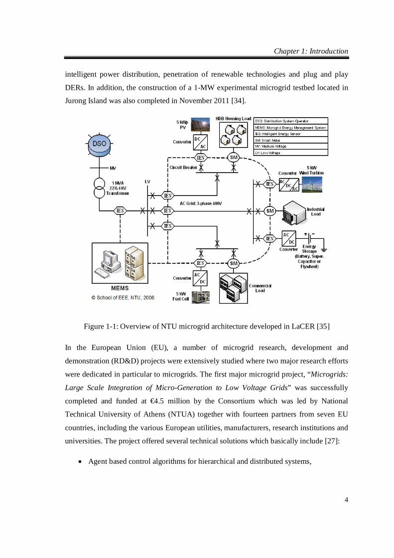
In terms of implementation, microgrid related research and development (R&D) activities
involving ongoing pilot projects and research related experimental setups which serve as a
testbed for microgrid R&D have been widely reported in many countries. In Singapore, a
SGD$1.32 million microgrid energy management system (MG-EMS) project funded by
the Agency for Science, Technology And Research (A*STAR) was completed by a team
of researchers at Nanyang Technological University (NTU) in July 2011 [34]. A schematic
illustrating the 0.4kV microgrid and the MicroGrid Energy Management System (MG-
EMS) developed in Laboratory for Clean Energy Research (LaCER) at NTU is shown in
Figure 1-1. The primary objective of this project was to design and develop software
algorithms, control schemes and hardware prototypes which are responsible for the
monitoring, control and decision-making in the management of microgrids. In addition, the
web based MG-EMS is also expected to perform several functions which mainly include
the prediction of total consumer loads, economic scheduling of DERs, active management
by rescheduling the real and reactive power, improving energy efficiency and thermal
energy utilization at distribution level. In addition, another SGD$38 million experimental
power grid center (EPGC) was also built as a research unit within the Agency for Science,
Technology and Research (A*STAR) to support the development of next generation grid
technology. The core focus of EPGC’s research is on challenges and issues related to
Chapter 1: Introduction
4
intelligent power distribution, penetration of renewable technologies and plug and play
DERs. In addition, the construction of a 1-MW experimental microgrid testbed located in
Jurong Island was also completed in November 2011 [34].
Figure 1-1: Overview of NTU microgrid architecture developed in LaCER [35]
In the European Union (EU), a number of microgrid research, development and
demonstration (RD&D) projects were extensively studied where two major research efforts
were dedicated in particular to microgrids. The first major microgrid project, “Microgrids:
Large Scale Integration of Micro-Generation to Low Voltage Grids” was successfully
completed and funded at €4.5 million by the Consortium which was led by National
Technical University of Athens (NTUA) together with fourteen partners from seven EU
countries, including the various European utilities, manufacturers, research institutions and
universities. The project offered several technical solutions which basically include [27]:
Agent based control algorithms for hierarchical and distributed systems,
Chapter 1: Introduction
5
DER modeling using steady-state and dynamic analysis in inverter-dominated
microgrids,
Intelligence requirements and interface response of DERs, and
Operating philosophies for interconnected and islanded microgrids.
The second major project, “More Microgrids: Advanced Architectures and Control
Concepts for More Microgrids” was funded at €8.5 million by a second Consortium which
was led by NTUA consisting of various manufacturers and power utilities based in Europe.
The main objectives [27] for this project include:
Developing alternative control strategies using next-generation information and
communication technologies,
Technical and commercial integration of multiple microgrids with upstream
distribution management systems that focuses on operation of decentralized energy
and ancillary service markets, and
Standardizing technical and commercial protocols to allow ease of installing DERs
with plug-and-play capabilities.
Several EU demonstration sites which showcase pilot microgrid installations were also
reported [27]. The first demonstration site is located in Kythnos Island, Greece where the
microgrid primarily consists of a 10kW PV system, 53kWh battery bank, 5kW diesel
genset and several residential loads and focuses on controlling the battery and PV
converters. The second pilot installation is in the Netherlands located in Continuon’s
MV/LV facility. This microgrid comprises some residential loads and a 315kW grid-tied
PV system and aims to manage PV power during peak and off-peak hours and the power
quality of the microgrid during islanded operation. The third demonstration site is located
in Germany under the MVV residential demonstration at Mannheim-Wallstadt where the
microgrid is composed of a 30kW PV system with some residential loads and is aimed at
engaging customers in load management. Other installation activities are also taking place
in Denmark, Italy, Portugal and Spain.
Chapter 1: Introduction
6
In the United States (U.S), there was a modest expansion of the microgrid research
program which was supported by the U.S. Department of Energy (DOE) and the California
Energy Commision (CEC). One of the well known U.S microgrid which was built by the
Consortium for Electric Reliability Technology Solutions (CERTS) in 1999 to investigate
the implications of emerging technologies, regulatory-institutional, economic and
environmental influences on power system reliability. The CERTS microgrid has been
proven to work well in both simulation and bench testing of a laboratory scale test system
in order to demonstrate the technical feasibility of the system [27]. Furthermore, an energy
manager design funded by CERTS was also proposed for microgrids [36]. In addition, a
US$4 million microgrid energy management framework managed by General Electric was
co-funded by DOE to develop and demonstrate the viability of microgrids [37, 38].
In Canada, microgrid research activities are mostly based on medium voltage (MV)
networks. These projects are usually done in collaboration with the electric utility
industries, manufacturers and stakeholders in integration and utilization of DERs. The
main objectives of the microgrid projects include:
Development of control algorithms and protection schemes for autonomous
operation,
Investigating the impacts of high DER penetration in existing power systems, and
Exploring the effects of communication technologies in host microgrid and DER
operations.
In addition, further collaborations with the electric utility industries were made to conduct
field tests and experiments on several aspects [27] such as
Autonomous operation of microgrids for remote areas,
Grid-connected microgrid operations,
Planned islanding operation of microgrids, and
Developing MV test line for testing prototypes and performance evaluation.
Chapter 1: Introduction
7
In Japan, the government has set targets to increase the contribution of renewable sources
such as solar and wind power into its existing national grid. In 2003, three proposed
microgrid projects located in Aomori, Aichi and Kyoto Prefectures were initiated by the
New Energy and Industrial Technology Development Organization (NEDO) to study the
integration of renewable energy sources into existing distribution networks. In addition,
NEDO also sponsored the demonstration in Sendai on the multiple Power Quality
Reliability (PQR) services which aims to show that multiple power quality levels can be
simultaneously supplied by the microgrid and to compare the cost benefit analysis of
multiple PQR services with conventional uninterruptable power supply (UPS) equipment.
There are also future collaborations between Shimizu Corporation and University of Tokyo
to develop a microgrid control system consisting of a 90kW and 350kW natural gas
gensets, four 100kW electric double layer capacitors and a 200kW NiMH battery bank
[27].
1.2 Microgrid Control Architectures
Control architecture of a power system can be broadly classified into two distinctive
categories which are centralized and decentralized controls. The main difference between
the two types of control lies in the management of tasks and responsibilities given to the
respective controllers. In a dynamic microgrid where DGs and loads typically have
different ownerships, variations in generation and demand raise challenges in forecasting.
They result in high levels of uncertainties. In addition, information on power quantity and
cost function of DGs and loads is also not readily known [39]. Therefore, appropriate
control schemes and coordination strategies are necessary for efficient microgrid
operations.
1.2.1 Centralized Control
The main idea of centralized control is using a central processing unit to collect,
consolidate and process all the measurement data from various devices in order to make
control decisions. A fully centralized control architecture usually consists of a dedicated
central controller which executes a range of functions such as gathering data, performing
Chapter 1: Introduction
8
calculation and optimization and determining control actions for all units. In addition, all
of these functions are done at a single point which requires an extensive communication
infrastructure for the central controller and controlled units to interact.
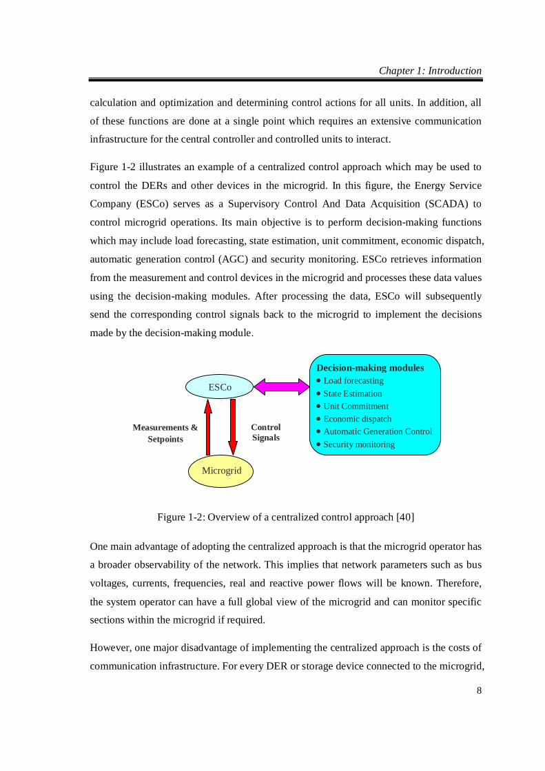
Figure 1-2 illustrates an example of a centralized control approach which may be used to
control the DERs and other devices in the microgrid. In this figure, the Energy Service
Company (ESCo) serves as a Supervisory Control And Data Acquisition (SCADA) to
control microgrid operations. Its main objective is to perform decision-making functions
which may include load forecasting, state estimation, unit commitment, economic dispatch,
automatic generation control (AGC) and security monitoring. ESCo retrieves information
from the measurement and control devices in the microgrid and processes these data values
using the decision-making modules. After processing the data, ESCo will subsequently
send the corresponding control signals back to the microgrid to implement the decisions
made by the decision-making module.
Figure 1-2: Overview of a centralized control approach [40]
One main advantage of adopting the centralized approach is that the microgrid operator has
a broader observability of the network. This implies that network parameters such as bus
voltages, currents, frequencies, real and reactive power flows will be known. Therefore,
the system operator can have a full global view of the microgrid and can monitor specific
sections within the microgrid if required.
However, one major disadvantage of implementing the centralized approach is the costs of
communication infrastructure. For every DER or storage device connected to the microgrid,
ESCo
Microgrid
Decision-making modules Load forecasting State Estimation Unit Commitment Economic dispatch Automatic Generation Control Security monitoring
Control Signals
Measurements & Setpoints
Chapter 1: Introduction
9
a corresponding set of control equipment to control the device must also be installed and
synchronized with the main microgrid server. This is particularly undesirable as most of
the DERs and energy storage devices are small in capacity and thus it may not be
economically feasible to individually control and govern each component at the microgrid
level. Furthermore, due to the need for processing large amounts of information at a single
point simultaneously, centralized control is unable to exhibit the plug-and-play feature
which is required in a dynamic microgrid setup. Consequently, this restricts power system
expansion and poses limitations on planning of power systems among other factors [41].
Although there are disadvantages associated with centralized control, it can, however, offer
broader observability of microgrid operations and greater knowledge for making control
decisions as part of its tradeoffs [42]. Generally, centralized control is more suited for
standalone power systems which need to maintain critical supply and demand balances in a
slow changing infrastructure with large generating units.
1.2.2 Decentralized Control
Decentralized or sometimes known as distributed control can be categorized into several
different types ranging from hybrid to a fully decentralized control. The main difference
between these control types lies in the responsibilities given to the controllers at various
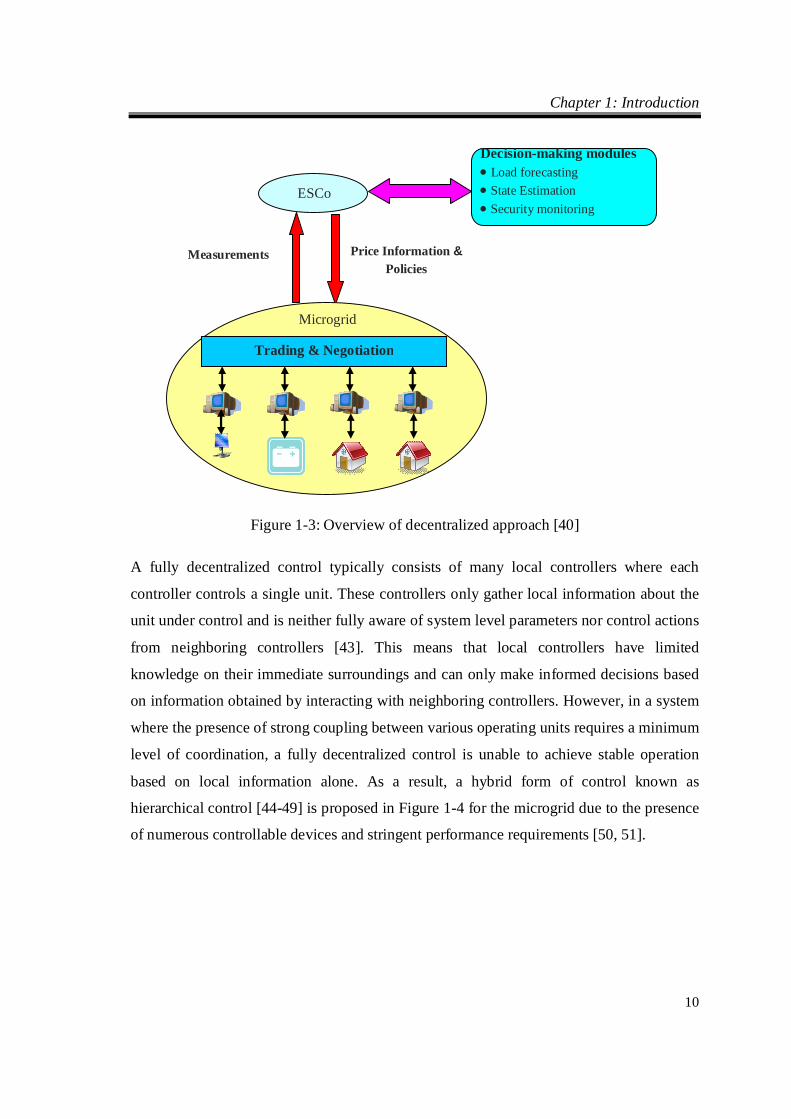
nodes within the microgrid. Figure 1-3 provides an overview on the operating principle for
the decentralized control approach. In this case, the ESCo provides basic ancillary services
such as load forecasting, state estimation and security monitoring. Economic dispatch,
scheduling and unit commitment are not included into the functions of ESCo because these
functions will be realized by the distributed controllers in the microgrid. The main role of
ESCo is to retrieve price information and policies from the utility grid. Together with the
decision making modules, this information is then sent to the clients (or agents) residing in
the microgrid where trading and negotiation will take place between the clients to obtain
the dispatch schedule for the respective DERs and storage devices. One observation from
this control architecture is that there is no single central processing server to implement
control decisions for all the local controllers. In this manner, information exchange
between ESCo and clients can be minimized.
Chapter 1: Introduction
10
Figure 1-3: Overview of decentralized approach [40]
A fully decentralized control typically consists of many local controllers where each
controller controls a single unit. These controllers only gather local information about the
unit under control and is neither fully aware of system level parameters nor control actions
from neighboring controllers [43]. This means that local controllers have limited
knowledge on their immediate surroundings and can only make informed decisions based
on information obtained by interacting with neighboring controllers. However, in a system
where the presence of strong coupling between various operating units requires a minimum
level of coordination, a fully decentralized control is unable to achieve stable operation
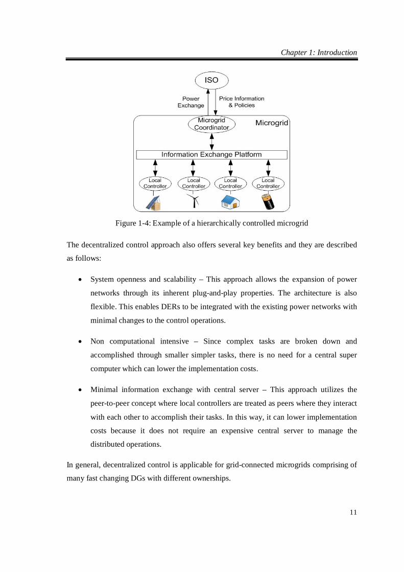
based on local information alone. As a result, a hybrid form of control known as
hierarchical control [44-49] is proposed in Figure 1-4 for the microgrid due to the presence
of numerous controllable devices and stringent performance requirements [50, 51].
ESCo
Decision-making modules Load forecasting State Estimation Security monitoring
Price Information & Policies
Measurements
Microgrid
Trading & Negotiation
Chapter 1: Introduction
11
Figure 1-4: Example of a hierarchically controlled microgrid
The decentralized control approach also offers several key benefits and they are described
as follows:
System openness and scalability – This approach allows the expansion of power
networks through its inherent plug-and-play properties. The architecture is also
flexible. This enables DERs to be integrated with the existing power networks with
minimal changes to the control operations.
Non computational intensive – Since complex tasks are broken down and
accomplished through smaller simpler tasks, there is no need for a central super
computer which can lower the implementation costs.
Minimal information exchange with central server – This approach utilizes the
peer-to-peer concept where local controllers are treated as peers where they interact
with each other to accomplish their tasks. In this way, it can lower implementation
costs because it does not require an expensive central server to manage the
distributed operations.
In general, decentralized control is applicable for grid-connected microgrids comprising of
many fast changing DGs with different ownerships.
Chapter 1: Introduction
12
1.3 Restructuring of the Power Industry
During the last few decades, the power industry scene has undergone major restructuring
which can be seen in many countries around the world. Traditionally, utilities were
predominantly monopolistic and vertically integrated but this structure is gradually giving
way to a new competitive environment where generation and distribution companies can
trade freely and have non-discriminatory access to the power network [18]. This
transformation is commonly termed as deregulation. A direct consequence of this is the
introduction of deregulated energy markets [52-61]. The objective of this market is to
consider energy as a commodity that can be freely traded and the energy price can be set
according to demand and supply at a particular period of time.
As a result of deregulation, several new entities were created in the electricity market
sector [18]. The first entity introduced is the generation companies (Gencos) which are
power generation companies who compete among themselves to sell power. Following that,
there are distribution companies (Discos) which purchase power from the wholesale
market and sell it to consumers. In addition, there is another group of transmission
companies (Transcos) which own the transmission network and direct power flow from
Gencos to Discos. The transactions that take place in deregulated electricity markets are
done through wholesale power markets which basically consist of a power exchange and
several power trading companies (Tradecos). Finally, other services that are required for
the secure and reliable operation of the power network are provided by an Independent
System Operator (ISO). In addition, the ISO also overlooks electricity market operation
and is accountable for the security and reliability standards in the power network.
The transition from regulation to deregulation contained several complexities and many
issues which need to be addressed. This is because of the unique characteristics inherent in
the power industry which hinders its successful commercialization [55]. The following
peculiarities of electricity are discussed below while designing electricity markets:
Energy storage issues – There is currently no cost effective ways for storing energy
on a large scale. This means that demand and supply need to be balanced
Chapter 1: Introduction
13
instantaneously. The power imbalance in the system has to be also promptly
balanced through some technical means.
Congestion management – The law of physics have a greater influence on the flow
of electricity within the power network than commercial contracts. Satisfying all
contracts may cause congestion in certain parts of the system.
Provision of ancillary services – The generation of energy and the provision of
ancillary services are interdependent in order to ensure that the power system is
stable and secure. These ancillary services may include frequency regulation,
operating reserves and reactive power compensation which are to be provided by
the same and other generating units.
Scheduling and dispatching generating units – There is a need to plan ahead the
scheduling of generating units and dispatch them in real time because electricity
travels quickly through transmission and distribution lines.
The architecture for electricity markets is more complicated compared to other commodity
markets due to the peculiarities in electricity as described previously. Experts also could
not arrive at a common agreement for designing the architecture of electricity markets
despite many years of operating experience. In many parts of the world, electricity markets
do not follow a common standard design because of the wide diversification in their
architectures. Electricity markets can be divided into several submarkets which are
classified into different categories depending on certain criteria. One common criterion
used to classify electricity markets is to identify the type of product being traded. Based on
this criterion, electricity markets are classified as follows:
Energy market – This market primarily deals with energy trading. The Market
Clearing Price (MCP) is computed from the submitted bids of the energy buyers
and energy sellers.
Transmission market – This market deals in the transmission rights which is
auctioned by the ISO. The transmission rights authorize the user to inject or
consume power from the transmission grid.
Ancillary service market – This market basically deals with ancillary services such
as frequency regulation, reactive power compensation and various forms of
Chapter 1: Introduction
14
reserves. The ancillary services provided by the ancillary service providers are to
be procured by the ISO.
Likewise, the electricity submarkets can be classified based on the degree of coordination
as described in the following:
Bilateral market – In this market, energy buyers and energy sellers enter into a
bilateral contract for the purchase and sale of power at an agreed price. This can be
done directly between sellers and buyers or through a broker. This type of market is
highly decentralized which limits the role of the ISO to verify the availability of
transmission capacity before completing any transactions.
Pool market – In this market, the ISO receives the submitted bids from generators
and loads and performs dispatch on them. This type of market is highly centralized
where the ISO has a larger role to play. In addition, the Locational Marginal Price
(LMP) is determined by the ISO by maximizing the social welfare of the generating
and load entities.
In addition, there are also other types of submarkets which include brokered, dealer and
exchange markets. In terms of architecture, these submarkets are also ranked according to
their hierarchy. Bilateral markets are classified as having a highly decentralized structure
followed by brokered markets, dealer markets, exchange markets and finally, pool markets
being the most centralized structure [18].
Furthermore, electricity submarkets can be categorized [18] based on the time of operation
which is described in the following:
Forward market – This market primarily handles long term and short term bilateral
contracts. Long term contracts are defined as procuring electricity over a long time
span which may range from several months to several years. Conversely, short term
contracts are defined as procuring electricity over a short time span which may
range from a few days to several weeks.
Spot market – This type of market is typically either day ahead which schedules
resources at every hour on the following day or hour ahead which schedules
Chapter 1: Introduction
15
resources for any deviation from the day ahead schedule. In addition, energy and
ancillary services may be traded in this market.
Real-time market – The generation and demand in a power system must be
balanced in real-time to ensure its reliability during normal operation. However,
there are instances when the real-time generation and demand deviate from the spot
market and forward market scheduling. To address this issue, real-time markets are
developed in order to meet the power balancing requirements in real-time.
Therefore, the three submarkets described above address energy trading and ancillary
services based on the time of operation. Chronologically, forward markets will be the first
submarket to award the contracts to successful bidders followed by the spot market and
finally, the real-time market to continuously balance the generation and demand of the
power system during the actual delivery period.
1.4 Research Motivation
The proliferation of renewable energy has changed the way energy is distributed and
consumed. The evolution in smart grid applications and energy management systems has
also gained momentum in recent years to better manage energy in a cost-effective manner
in view of rising oil prices. In Singapore, the Energy Market Authority (EMA) is currently
reviewing its existing regulatory framework to facilitate the deployment of renewable
sources and their integration into the current electricity market [62]. In addition, the energy
policy in Singapore also emphasized on fostering greater competition in the power market
to ensure electricity prices remain competitive. Several initiatives were recently announced
in 2013 in which one of them highlights the introduction of electricity futures market to
complement the existing spot market. Another initiative was also proposed which
introduces a demand response scheme to allow consumers to curtail demand when
electricity prices are high and is expected to commence in 2015. The primary objective of
these initiatives is to foster a competitive electricity market structure which empowers
consumers with more choices and for end users to create a diversified portfolio for
electricity and demand to reduce volatility.
Chapter 1: Introduction
16
Due to the anticipated increase in penetration of Distributed Energy Resources (DERs) at
the microgrid level, control and management are necessary to ensure smooth and stable
operation of microgrids. However, traditional centralized intelligence approaches proved to
be inadequate to cope with the increasing growth of DERs due to the lack of flexibility and
extensibility [63]. Moreover, centralized control was initially designed to handle large
generation units. With numerous DERs appearing in the power network, it is difficult or
nearly impossible to control the entire system by a single central controller adopting a top-
down approach [64, 65]. If such a controller is implemented, it would require increased
cost for communication infrastructure and introduce added complexity in the centralized
control supervisor.
Similarly, power market operations and distribution networks become increasingly
complex as the power industry moves towards decentralization [66]. The presence of
DERs at distribution voltage levels will inevitably change the way power flows within the
network causing it to change from a passive to an active one. Consequently, centralized
Supervisory Control and Data Acquisiton (SCADA) which was originally designed for
traditional passive networks may be inadequate to cope with the high penetration of DERs
and complex control decisions [63]. In addition, the assumptions applied to conventional
power systems may not be valid for active distributed systems which raise challenges in
the operation of microgrids [39]. The main issues regarding integration of DERs are also
highlighted in [67-70] which primarily include:
The need for scheduling and dispatch of DGs under supply and demand
uncertainties,
Design of new market models that enables competitive participation within a
microgrid,
Development of market and control mechanisms which exhibits plug-and-play for
seamless integration of DERs,
Cooperation and control which are distributed and realized with minimal
information exchange with the central controller, and
Communication networks which are based on standard components such as TCP/IP
protocol.
Chapter 1: Introduction
17
Most of the above mentioned issues can be addressed by providing an agent platform with
a common communication interface in the distributed system [71]. This can be realized by
MAS which has been widely proposed as a feasible approach for managing distributed
systems because it can effectively handle complex systems operations by decomposing
complex tasks into simpler tasks to accomplish its goals [72-74]. The extension of MAS
into microgrid applications is also evident in [74-91] where various research activities
ranging from agent based market operation, fault protection strategies, DG control
schemes, coordination control strategies, optimization strategies and distributed energy
management systems to real time implementations.
MAS is a form of decentralized control which exhibits distributed intelligence by
employing software entities or agents to communicate, negotiate and optimize microgrid
operations. As opposed to the centralized approach, MAS uses a bottom-up approach to
manage and optimize microgrid operations so that communications and complexity of the
microgrid are kept to minimal. In addition, proposed guidelines and requirements on the
use and applications of MAS in power systems are discussed in detail [92, 93]. Key
motivation for proposing MAS in power systems basically lies in its inherent benefits such
as flexibility, scalability, autonomy and reduction in problem complexity among other
factors.
Therefore, the motivation of this thesis is to develop an agent based distributed control
scheme for optimizing microgrid operations. The integration of DGs into the distribution
grid will ultimately change the way power flows within the network. This calls for a need
to better manage the power flow as well as market operations. In addition, the DGs and
loads may have different ownerships and operating objectives which may result in
conflicting goals among themselves. A local competitive microgrid market is proposed and
developed in this thesis which considers the individual objectives of each participant. The
impacts of different operating objectives for DGs and loads are also examined and
discussed. This can help cater to the needs of individual power producers (IPPs) and price
conscious consumers so that they can satisfy their respective objectives and at the same
time, help to drive down local energy costs and maximize the overall benefit of the
microgrid.
Chapter 1: Introduction
18
1.5 Objectives of the Research
In this thesis, the research focus is to examine how the microgrid can be best managed
based on price-sensitive generation sources and loads. A multi agent based optimization
control scheme based on a hierarchical architecture is proposed to investigate how such a
proposed scheme can be adapted to best fit the operation needs of microgrids while
maximizing their revenue when connected to upstream networks. Three main objectives
have been identified and are described as follows.
The first objective in this thesis is to design and build a multi agent system (MAS)
platform for microgrid operations. The MAS platform is designed to perform the following:
Execute market operations for microgrids using the proposed market clearing
algorithm;
Simulate agent interaction and coordination based on different agent objectives,
Send real-time control signals to the generators and loads in order to regulate their
power set points;
All the above actions are coordinated through a series of agent communication and
coordination.
The second objective is to investigate how different market mechanisms and agent
objectives will affect microgrid operations. Two types of market mechanisms will be
considered: 1) A single side bidding whereby generators are allowed to bid and, 2) a
double side bidding whereby both generators and loads are allowed to bid. Besides, the
agent objectives are categorized into two types i.e. cooperative and competing. By
studying the market outcomes based on different agent objectives, the optimal market
results and agent objectives can be evaluated.
The final objective is to implement the outcome of the market operations on a simulated
real-time environment in order to verify the proper operation of the microgrid. The
microgrid is modeled in Matlab/Simulink environment and the agents are communicating
to the Matlab/Simulink models via MACSimJX. The micogrid is simulated for a 24-hour
period where the market clears every hourly. The output active power and voltage
Chapter 1: Introduction
19
waveforms for the generators and loads will be analyzed to evaluate the performance of the
agent based control scheme for microgrids.
1.6 Organization of Thesis
This thesis is organized into five chapters. The current chapter, which is Chapter 1,
provides an introduction to the deregulation and restructuring of the power industry. The
concept of microgrid and various microgrid control schemes are introduced. Trends in
microgrid technologies and recent developments are also reviewed. It also reviews the
problems and challenges faced when employing conventional centralized control in
microgrids and the need for distributed controls in the management of microgrids. A
hybrid form of control, also known as hierarchical control, and its architecture for
microgrids are introduced. The research motivation, objectives and organization of this
thesis are also discussed.
Chapter 2 provides a literature review on Multi Agent Systems and its application in
microgrid operations. The agent theory, concepts and architecture are introduced and
described in detail. In addition, the IEEE Foundation for Intelligent Physical Agent (FIPA)
standard for agents is introduced. This provides standards for agent design and
implementation. The Java based agent framework is subsequently introduced that provides
an IEEE FIPA compliant platform for agent implementation. This framework is further
extended to Matlab/Simulink using multi agent control for simulink with JADE extension
(MACSimJX) and its working principle and architecture are also presented.
Chapter 3 presents a preliminary agent design for microgrid operation. It discusses the use
of JADE to simulate agent control for scheduling and dispatch of DGs in a microgrid based
on market pricing. A list of agents that are developed and customized according to the
requirements of the microgrid has been discussed. In addition, the functions of these agents
are described in detail. Agent implementation in JADE relies on agent communication and
message exchanges in order to fulfill their objectives. In the simulation studies, agent
communication is demonstrated through the trading and negotiation process. Simulation
studies have been done to analyze the performance of the customized agents under grid
Chapter 1: Introduction
20
connected mode of operations. Simulation results have shown that the agents developed
are capable of performing decentralized microgrid control operations.
Chapter 4 presents a proposed Multi Agent System approach for integrating microgrid
market operations and DER implementations. In this approach, each DG or price-sensitive
load is modeled as an energy seller or energy buyer respectively and is represented by an
agent which participates in a microgrid energy market. Each agent aims at maximizing the
benefits according to the defined agent objectives while ensuring the smooth operation and
proper execution of microgrid operations under a simulated real-time environment. The
results from simulation studies demonstrate the effectiveness in employing multi agent
system to perform coordinated actions between market operations and DER
implementations in the distributed management of microgrids.
Chapter 5 provides conclusion, contributions of this thesis and suggestions on future works
with regards to the research of multi agent systems for distributed microgrid operations.
Chapter 2: Introduction to Multi Agent Systems (MAS)
21
CHAPTER 2 INTRODUCTION TO MULTI AGENT SYSTEM (MAS)
A multi agent system (MAS) typically consists of a collection of two or more objective-
oriented agents interacting with each other to solve complex problems in a distributed
manner. The term agent refers to either a software abstraction, idea or concept containing
methods and objects which provide an intuitive way to describe complex software entities
that are able to act with a certain level of autonomy to complete some designated tasks. An
agent may also be defined in terms of its behavior but several authors have proposed
different variation of agent definitions in the past. Although the agent definition varies
from different sources, there are several key concepts which are common among these
agent definitions and they are 1) sociability, 2) autonomous, and 3) reactivity. Based on
these key concepts, an agent can then be defined as either a software or hardware entity
operating in an environment with a certain level of autonomy, knowledge and specified
goals.
A more general definition of an agent is also provided in [94] which basically defines an
agent as an autonomous entity that can either communicate with other agents or solve
problems on its own in an embedded environment. In addition, agents are able to control
its internal state and outputs. They can also operate without external human intervention.
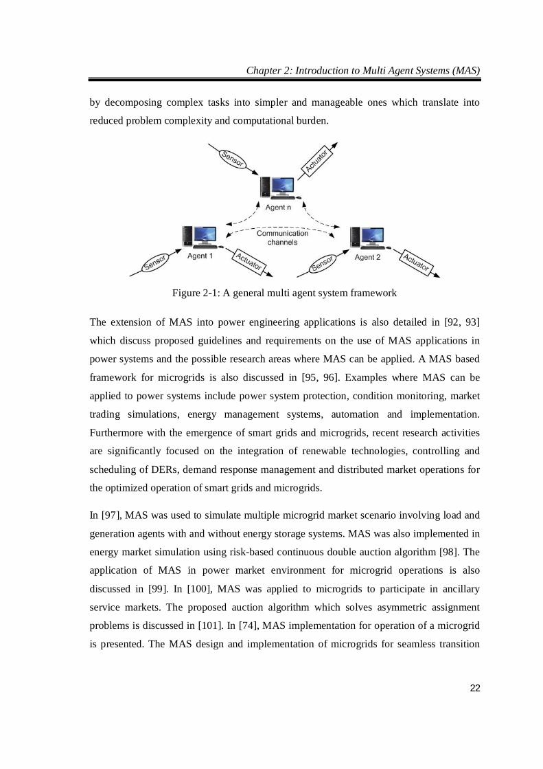
Figure 2-1 illustrates a general MAS framework conceptually. In this figure, each agent is
equipped with the relevant tools such as sensors and actuators to obtain local data and
provide control signals to the equipment respectively. In addition, agents may also interact
with each other by exchanging messages in order to achieve specified objectives.
Inherently, MAS offers several desirable key features which include 1) the ability to
parallel process, 2) scalability, 3) modularity, 4) flexibility, 5) extensibility, 6) reliability
and 7) the capability to represent, model and control distributed systems which make MAS
the ideal candidate for a wide range of engineering applications. In the past few decades,
MAS has been widely applied in many areas which include traffic and transport
optimization, aircraft controls, robotics, medicine, commerce, congestion control and
power systems control. The main objective of MAS is to solve complex dynamic problems
Chapter 2: Introduction to Multi Agent Systems (MAS)
22
by decomposing complex tasks into simpler and manageable ones which translate into
reduced problem complexity and computational burden.
Figure 2-1: A general multi agent system framework
The extension of MAS into power engineering applications is also detailed in [92, 93]
which discuss proposed guidelines and requirements on the use of MAS applications in
power systems and the possible research areas where MAS can be applied. A MAS based
framework for microgrids is also discussed in [95, 96]. Examples where MAS can be
applied to power systems include power system protection, condition monitoring, market
trading simulations, energy management systems, automation and implementation.
Furthermore with the emergence of smart grids and microgrids, recent research activities
are significantly focused on the integration of renewable technologies, controlling and
scheduling of DERs, demand response management and distributed market operations for
the optimized operation of smart grids and microgrids.
In [97], MAS was used to simulate multiple microgrid market scenario involving load and
generation agents with and without energy storage systems. MAS was also implemented in
energy market simulation using risk-based continuous double auction algorithm [98]. The
application of MAS in power market environment for microgrid operations is also
discussed in [99]. In [100], MAS was applied to microgrids to participate in ancillary
service markets. The proposed auction algorithm which solves asymmetric assignment
problems is discussed in [101]. In [74], MAS implementation for operation of a microgrid
is presented. The MAS design and implementation of microgrids for seamless transition
Chapter 2: Introduction to Multi Agent Systems (MAS)
23
from grid-connected to islanded mode in MATLAB/Simulink environment is discussed in
[75, 102].
2.1 Autonomous Agents
MAS is made up of many agents interacting with one another to achieve a common goal.
Each agent is specifically assigned with tasks and responsibilities and is required to
communicate with other agents to achieve its objectives. In addition, agents are also
expected to have self autonomy and exhibit intelligence which is one of the important
characteristics of intelligent agents. This means that agents should be capable of deciding
the next course of action for the equipment they are controlling without any form of major
intervention from either the owner or the main central server. It is particularly useful in the
context of microgrids because with numerous DERs connected to the microgrid network,
control operations will not be delayed if any DER fails to respond. Agents should also be
able to adjust accordingly to different circumstances. Some important key attributes of
agents are listed [103, 104] as follows:
Social ability - Since agents have partial or no knowledge of the entire network,
agents are required to communicate with one another to achieve their objectives.
Through communication with neighboring agents, each agent can continuously
update itself with relevant information.
Reactivity - Agents are programmed in such a way that they can respond and adapt
to any changes in the environment without much delay. For instance, if any DER
agents goes offline due to either a fault or maintenance, neighboring agents can be
notified and subsequently make minor adjustments in their behaviors to ensure that
the system continues to operate smoothly.
Pro-activeness - Agents alone cannot achieve their objectives unless they take the
initiative to interact with other agents. In order to accomplish their objectives,
agents should exhibit goal-directed behaviors and actively engage in interaction
with other agents.
Chapter 2: Introduction to Multi Agent Systems (MAS)
24
Reliability - Agents are not allowed to intentionally provide false or misleading
information that can potentially corrupt the integrity of the information exchanged
between agents.
Mobility - Agents are able to migrate from one host platform to another without
requiring a major overhaul to the existing system. This property is desirable
because when a client computer is scheduled for maintenance, agents can
temporary migrate to another client without causing any downtime for the
equipment it is controlling. Agents are the fundamental building block which drives MAS applications. They are
particularly effective when they work together in groups because they can potentially
improve systems operating on artificial intelligence. Therefore, it is important to
understand and appreciate the underlying principles of agent theory for agent design and
development. Various agent theories which attempt to capture different aspects of
intelligent behaviors are discussed in [94]. In the following sections, some agent theories
which attempt to capture different aspects of intelligent behaviors that can result in varying
degrees of intelligence are discussed.
2.1.1 The theory of intention
One possible way for an agent to achieve a task is by providing it with a set of intentions.
It is closely affiliated to the goal-directed, purposeful and behavior inherent in living
organisms. P. R. Cohen and H. J. Levesque [105] believe that six properties need to be
satisfied for any theory which discusses intentions and they are described as follows:
Intentions create problems where agents need to find ways of achieving them.
New intentions must not overlap and/or conflict with existing intentions.
Agents are goal-oriented and will attempt to try again until they succeed in
achieving their intentions.
Agents believe that the intentions given to them are achievable.
Chapter 2: Introduction to Multi Agent Systems (MAS)
25
Agents always believe in the success of their intention where failure is not an
option.
Agents cannot foresee the consequences of their intentions.
In addition, they [105] believe that agents have persistent goals if two criteria are met as
follows:
The goal will ultimately become true even though it is not true at present.
Before deciding to drop any goals, agents believe that the goal is either satisfied or
will never be satisfied [106].
Agents that have intentions can be interpreted as having a strong motivation to achieve a
certain desired state. This means that agents have to find ways to change a current state
into a desired future state. In the context of control systems, the future state can be seen as
a setpoint for the controller which it constantly wants to achieve. While it is desirable for
agents to have intentions, they must also be intelligent enough to recognize whether an
objective is impossible to achieve. This is because agents will exhibit obsessional
behaviour if they try to achieve an objective that is impossible which will lead to
unproductive outcomes that is undesirable.
2.1.2 The Possible Worlds Model
Another possible way for an agent to achieve its tasks is by developing a set of solutions
based on its own beliefs. J. Hintikka [107] developed this model as a means to represent
the knowledge and beliefs held by agents. This model works well with the intention theory
because it considers the methods and/or strategies required to accomplish objectives. The
strategies are known as worlds in this model and are represented in a system using classical
propositional logic. The theory of this model states that the set of possible strategies
developed for any given situation is dependent on the beliefs and information that is
processed by the system. This means that the effectiveness of the strategies will increase
with more system information and thus improving the chances of accomplishing any given
Chapter 2: Introduction to Multi Agent Systems (MAS)
26
objectives. However, a limitation of this model is when system information is fixed and
predetermined resulting in a closed knowledge and belief system.
This problem can be solved if the system is capable of obtaining new relevant knowledge
to better improve strategies. This implies that the system must have the ability to monitor
its performance and learn from past experience. In addition, C. R. Robinson [94] also
suggested that language played an important role in the thinking and reasoning process of
agents which could possibly manipulate information stored in the memory and could think
about the consequences of their actions before executing the strategies. Therefore, the
prediction of future events and creation of better strategies can be done through the use of
language which appears to be important in learning concepts and the abstraction of rules.
2.1.3 Belief Desire Intention (BDI) Model
Currently, this is the one of the more popular theories in agent based systems proposed by
A. S. Rao and M. P. Georgeff [108]. The theory in this model is derived from the intention
theory and is based on the branching concept of time. The primary motivation behind this
theory is to investigate how beliefs about the future will affect the desires and intentions of
agents. This implies that the agent will abandon a particular objective if it has beliefs about
the future that the objective is impossible to accomplish. Hence, this addresses the issue of
obsessional behavior previously discussed in the intention theory.
2.1.4 The Knowledge and Action Theory
This theory was proposed by R. Moore [109] which takes into account information that an
agent needs to know before taking any actions. The logical structure of this theory
considers the case when agents have incomplete information on how to go about
accomplishing their goals and provide procedures for them to search for additional
information which they require.
Chapter 2: Introduction to Multi Agent Systems (MAS)
27
2.1.5 Miscellaneous Theories
Other theories worth mentioning can be found in [110-113]. In [111], M. Wooldridge
developed a set of formalisms to describe a generalized model of a MAS. In [112], E.
Werner created an agent based system which uses the working principle of game theory,
economics, philosophy, situation semantics and situated automata theory. In [113], M.
Singh developed a set of formalisms in branching time framework using beliefs, intention,
communication and knowledge.
However, there is one common problem among these theories. They only address specific
behavorial features and functional attributes performed by agents. This implies that a more
comprehensive theory is needed to cover every aspect of agent behaviors and functional
attributes which will result in a system with higher degree of intelligence and is
particularly desirable in the design of MAS. However, such a theory has yet to be
developed. But over the years, developments in agent architectures have incorporated some
aspects of these theories which are discussed in the subsequent sections.
2.2 Agent Architectures
This section discusses the contribution of agent theories in the structuring of software
based MAS. While many different agent architectures have been discussed in [94], three
commonly used agent architectures are selected and described in the following sections in
order to illustrate the implementation of agent theory in agent architectures.
2.2.1 Deliberative-based Agents
An agent architecture is known to be deliberative or cognitive if it consists of an explicitly
represented symbolic model of the world. In this architecture, decisions are made through
logical reasoning which is based on symbolic manipulation and pattern matching. Agents
having this architecture will be able to consider alternative ways of solving a given
problem which may also include tapping on knowledge gained from past experiences.
Chapter 2: Introduction to Multi Agent Systems (MAS)
28
2.2.2 Reactive-based Agents
This architecture can be defined as having no memory to make decisions. This means that
reactive agents are designed such that the choice of action is situationally determined i.e.
they are programmed to perform certain actions based on a particular environmental
condition [114]. Agents respond immediately to changes in the environment by making
decisions based on the limited available information at that time. The primary advantage of
a reactive over a deliberative agent architecture is that it has a faster response time and
implementation is relatively easier. On the other hand, the disadvantage of reactive based
agent architecture is that the agent intelligence is limited because of the limited amount of
information available during decision making. In addition, several well known examples of
reactive agent architectures such as the subsumption architecture, Pengi, situated automata
and agent network architecture can also be found in [94] which describes each of them in
detail.
2.2.3 Hybrid-based Agents
This architecture is developed based on the combination of deliberative and reactive
properties mentioned previously. Typically, this architecture consists of many layers where
agents residing in the lower layers are assigned reactive behaviors which are responsible
for short term decision making. On the other hand, agents residing in the upper layers have
cognitive behaviors which are responsible for guiding the system towards the long term
goals. In [94], C. R. Robinson suggested that in terms of abilities, hybrid agents were
considered the most versatile among other architectures. Furthermore, several examples of
hybrid agents such as procedural reasoning system, touring machines, COSY and
inteRRaP are also described in detail.
2.3 Structure of an Agent
A typical agent structure is shown in Figure 2-2 which illustrates an example of a layered
architecture of an intelligent agent. An agent basically has a three-layered architecture
which includes the message handling layer, behavioral layer and the functional layer [115].
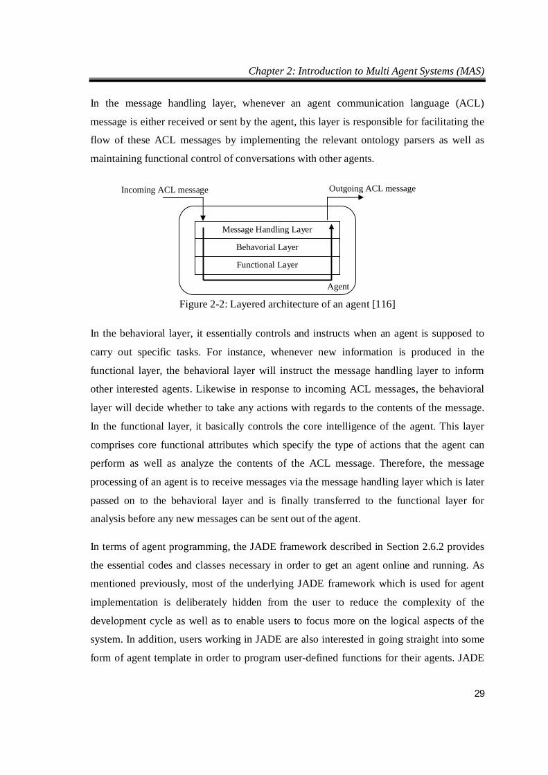
Chapter 2: Introduction to Multi Agent Systems (MAS)
29
Message Handling Layer
Behavorial Layer
Functional Layer
Incoming ACL message Outgoing ACL message
Agent
In the message handling layer, whenever an agent communication language (ACL)
message is either received or sent by the agent, this layer is responsible for facilitating the
flow of these ACL messages by implementing the relevant ontology parsers as well as
maintaining functional control of conversations with other agents.
Figure 2-2: Layered architecture of an agent [116]
In the behavioral layer, it essentially controls and instructs when an agent is supposed to
carry out specific tasks. For instance, whenever new information is produced in the
functional layer, the behavioral layer will instruct the message handling layer to inform
other interested agents. Likewise in response to incoming ACL messages, the behavioral
layer will decide whether to take any actions with regards to the contents of the message.
In the functional layer, it basically controls the core intelligence of the agent. This layer
comprises core functional attributes which specify the type of actions that the agent can
perform as well as analyze the contents of the ACL message. Therefore, the message
processing of an agent is to receive messages via the message handling layer which is later
passed on to the behavioral layer and is finally transferred to the functional layer for
analysis before any new messages can be sent out of the agent.
In terms of agent programming, the JADE framework described in Section 2.6.2 provides
the essential codes and classes necessary in order to get an agent online and running. As
mentioned previously, most of the underlying JADE framework which is used for agent
implementation is deliberately hidden from the user to reduce the complexity of the
development cycle as well as to enable users to focus more on the logical aspects of the
system. In addition, users working in JADE are also interested in going straight into some
form of agent template in order to program user-defined functions for their agents. JADE
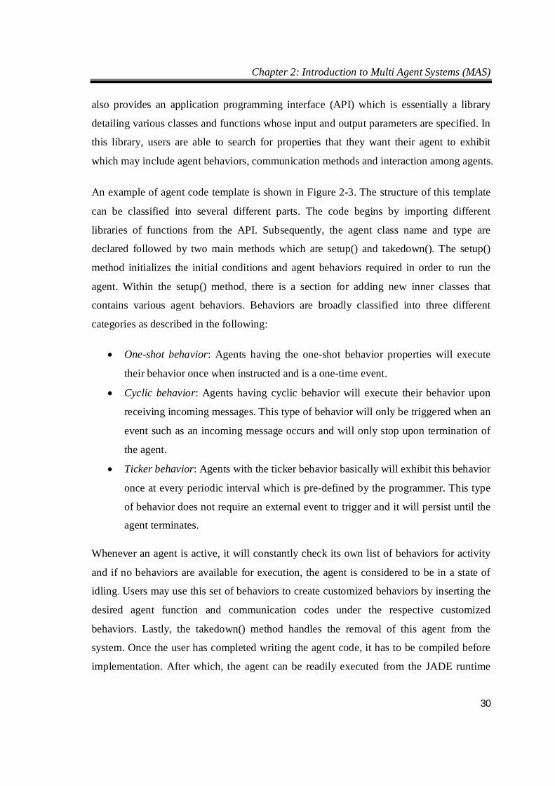
Chapter 2: Introduction to Multi Agent Systems (MAS)
30
also provides an application programming interface (API) which is essentially a library
detailing various classes and functions whose input and output parameters are specified. In
this library, users are able to search for properties that they want their agent to exhibit
which may include agent behaviors, communication methods and interaction among agents.
An example of agent code template is shown in Figure 2-3. The structure of this template
can be classified into several different parts. The code begins by importing different
libraries of functions from the API. Subsequently, the agent class name and type are
declared followed by two main methods which are setup() and takedown(). The setup()
method initializes the initial conditions and agent behaviors required in order to run the
agent. Within the setup() method, there is a section for adding new inner classes that
contains various agent behaviors. Behaviors are broadly classified into three different
categories as described in the following:
One-shot behavior: Agents having the one-shot behavior properties will execute
their behavior once when instructed and is a one-time event.
Cyclic behavior: Agents having cyclic behavior will execute their behavior upon
receiving incoming messages. This type of behavior will only be triggered when an
event such as an incoming message occurs and will only stop upon termination of
the agent.
Ticker behavior: Agents with the ticker behavior basically will exhibit this behavior
once at every periodic interval which is pre-defined by the programmer. This type
of behavior does not require an external event to trigger and it will persist until the
agent terminates.
Whenever an agent is active, it will constantly check its own list of behaviors for activity
and if no behaviors are available for execution, the agent is considered to be in a state of
idling. Users may use this set of behaviors to create customized behaviors by inserting the
desired agent function and communication codes under the respective customized
behaviors. Lastly, the takedown() method handles the removal of this agent from the
system. Once the user has completed writing the agent code, it has to be compiled before
implementation. After which, the agent can be readily executed from the JADE runtime
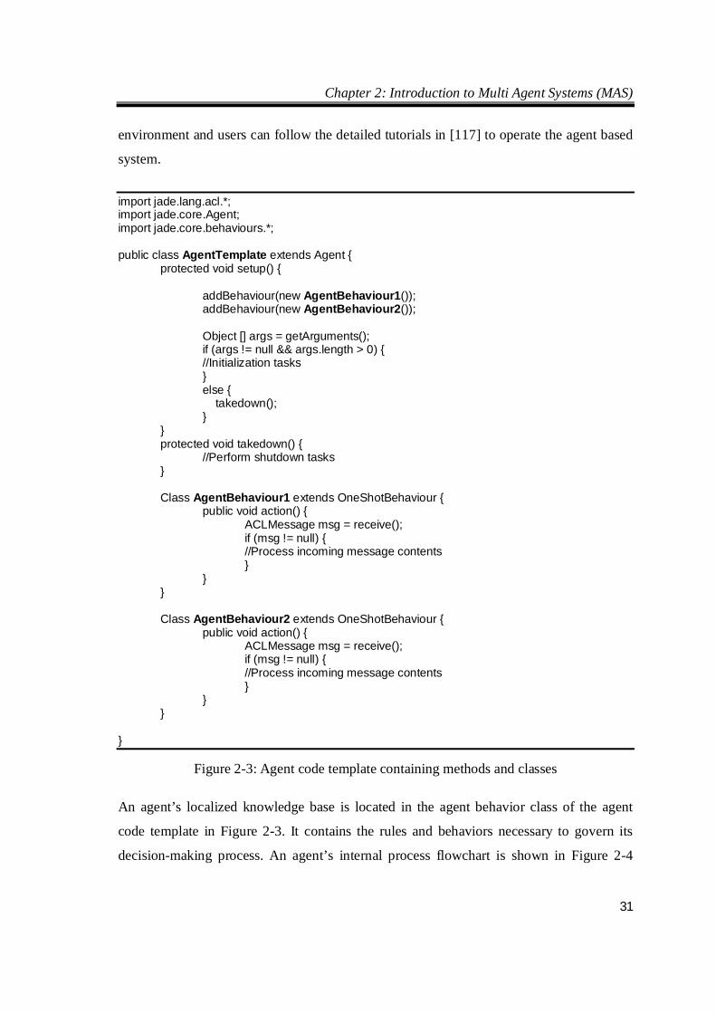
Chapter 2: Introduction to Multi Agent Systems (MAS)
31
environment and users can follow the detailed tutorials in [117] to operate the agent based
system.
import jade.lang.acl.*; import jade.core.Agent; import jade.core.behaviours.*; public class AgentTemplate extends Agent protected void setup()
addBehaviour(new AgentBehaviour1()); addBehaviour(new AgentBehaviour2());
Object [] args = getArguments(); if (args != null && args.length > 0) //Initialization tasks else takedown(); protected void takedown() //Perform shutdown tasks Class AgentBehaviour1 extends OneShotBehaviour public void action() ACLMessage msg = receive(); if (msg != null) //Process incoming message contents
Class AgentBehaviour2 extends OneShotBehaviour public void action() ACLMessage msg = receive(); if (msg != null) //Process incoming message contents
Figure 2-3: Agent code template containing methods and classes
An agent’s localized knowledge base is located in the agent behavior class of the agent
code template in Figure 2-3. It contains the rules and behaviors necessary to govern its
decision-making process. An agent’s internal process flowchart is shown in Figure 2-4
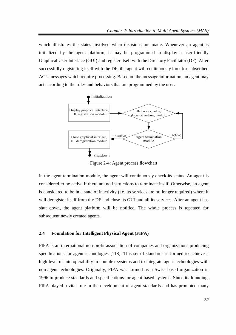
Chapter 2: Introduction to Multi Agent Systems (MAS)
32
which illustrates the states involved when decisions are made. Whenever an agent is
initialized by the agent platform, it may be programmed to display a user-friendly
Graphical User Interface (GUI) and register itself with the Directory Facilitator (DF). After
successfully registering itself with the DF, the agent will continuously look for subscribed
ACL messages which require processing. Based on the message information, an agent may
act according to the rules and behaviors that are programmed by the user.
Figure 2-4: Agent process flowchart
In the agent termination module, the agent will continuously check its status. An agent is
considered to be active if there are no instructions to terminate itself. Otherwise, an agent
is considered to be in a state of inactivity (i.e. its services are no longer required) where it
will deregister itself from the DF and close its GUI and all its services. After an agent has
shut down, the agent platform will be notified. The whole process is repeated for
subsequent newly created agents.
2.4 Foundation for Intelligent Physical Agent (FIPA)
FIPA is an international non-profit association of companies and organizations producing
specifications for agent technologies [118]. This set of standards is formed to achieve a
high level of interoperability in complex systems and to integrate agent technologies with
non-agent technologies. Originally, FIPA was formed as a Swiss based organization in
1996 to produce standards and specifications for agent based systems. Since its founding,
FIPA played a vital role in the development of agent standards and has promoted many
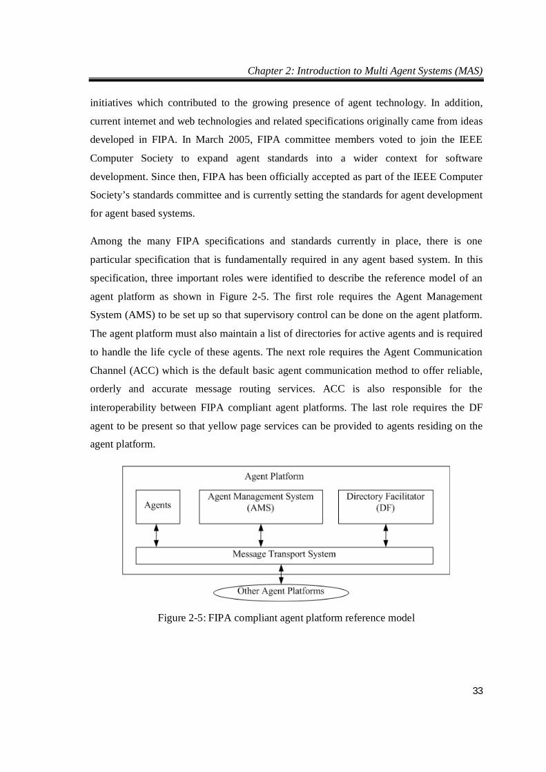
Chapter 2: Introduction to Multi Agent Systems (MAS)
33
initiatives which contributed to the growing presence of agent technology. In addition,
current internet and web technologies and related specifications originally came from ideas
developed in FIPA. In March 2005, FIPA committee members voted to join the IEEE
Computer Society to expand agent standards into a wider context for software
development. Since then, FIPA has been officially accepted as part of the IEEE Computer
Society’s standards committee and is currently setting the standards for agent development
for agent based systems.
Among the many FIPA specifications and standards currently in place, there is one
particular specification that is fundamentally required in any agent based system. In this
specification, three important roles were identified to describe the reference model of an
agent platform as shown in Figure 2-5. The first role requires the Agent Management
System (AMS) to be set up so that supervisory control can be done on the agent platform.
The agent platform must also maintain a list of directories for active agents and is required
to handle the life cycle of these agents. The next role requires the Agent Communication
Channel (ACC) which is the default basic agent communication method to offer reliable,
orderly and accurate message routing services. ACC is also responsible for the
interoperability between FIPA compliant agent platforms. The last role requires the DF
agent to be present so that yellow page services can be provided to agents residing on the
agent platform.
Figure 2-5: FIPA compliant agent platform reference model
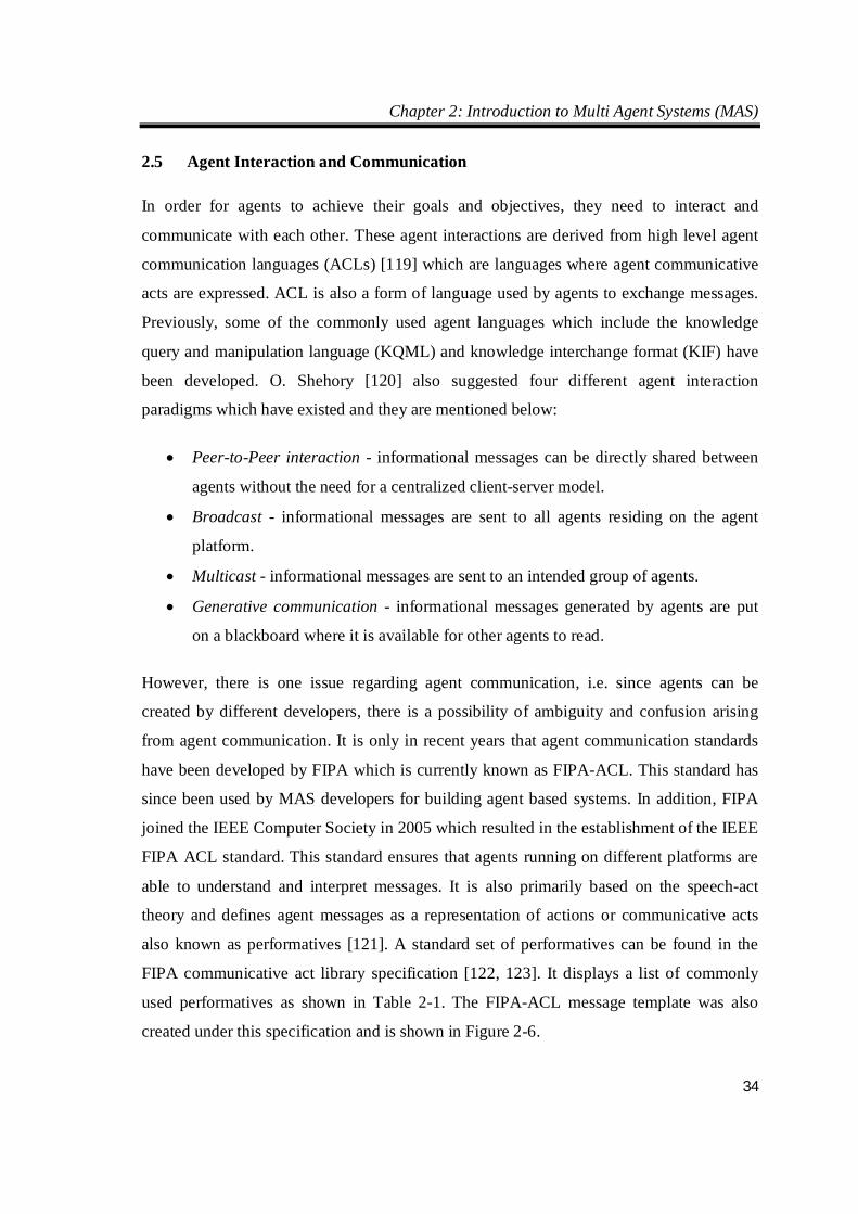
Chapter 2: Introduction to Multi Agent Systems (MAS)
34
2.5 Agent Interaction and Communication
In order for agents to achieve their goals and objectives, they need to interact and
communicate with each other. These agent interactions are derived from high level agent
communication languages (ACLs) [119] which are languages where agent communicative
acts are expressed. ACL is also a form of language used by agents to exchange messages.
Previously, some of the commonly used agent languages which include the knowledge
query and manipulation language (KQML) and knowledge interchange format (KIF) have
been developed. O. Shehory [120] also suggested four different agent interaction
paradigms which have existed and they are mentioned below:
Peer-to-Peer interaction - informational messages can be directly shared between
agents without the need for a centralized client-server model.
Broadcast - informational messages are sent to all agents residing on the agent
platform.
Multicast - informational messages are sent to an intended group of agents.
Generative communication - informational messages generated by agents are put
on a blackboard where it is available for other agents to read.
However, there is one issue regarding agent communication, i.e. since agents can be
created by different developers, there is a possibility of ambiguity and confusion arising
from agent communication. It is only in recent years that agent communication standards
have been developed by FIPA which is currently known as FIPA-ACL. This standard has
since been used by MAS developers for building agent based systems. In addition, FIPA
joined the IEEE Computer Society in 2005 which resulted in the establishment of the IEEE
FIPA ACL standard. This standard ensures that agents running on different platforms are
able to understand and interpret messages. It is also primarily based on the speech-act
theory and defines agent messages as a representation of actions or communicative acts
also known as performatives [121]. A standard set of performatives can be found in the
FIPA communicative act library specification [122, 123]. It displays a list of commonly
used performatives as shown in Table 2-1. The FIPA-ACL message template was also
created under this specification and is shown in Figure 2-6.
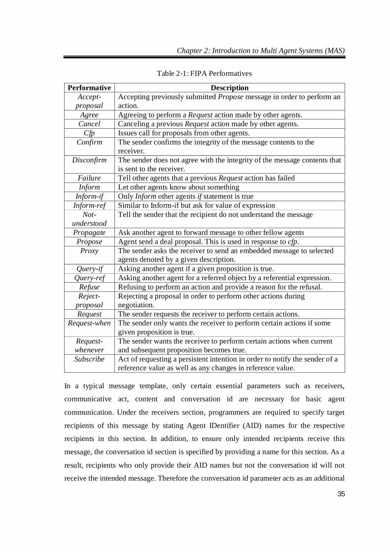
Chapter 2: Introduction to Multi Agent Systems (MAS)
35
Table 2-1: FIPA Performatives
Performative Description Accept-
proposal Accepting previously submitted Propose message in order to perform an action.
Agree Agreeing to perform a Request action made by other agents. Cancel Canceling a previous Request action made by other agents.
Cfp Issues call for proposals from other agents. Confirm The sender confirms the integrity of the message contents to the
receiver. Disconfirm The sender does not agree with the integrity of the message contents that
is sent to the receiver. Failure Tell other agents that a previous Request action has failed Inform Let other agents know about something
Inform-if Only Inform other agents if statement is true Inform-ref Similar to Inform-if but ask for value of expression
Not-understood
Tell the sender that the recipient do not understand the message
Propagate Ask another agent to forward message to other fellow agents Propose Agent send a deal proposal. This is used in response to cfp. Proxy The sender asks the receiver to send an embedded message to selected
agents denoted by a given description. Query-if Asking another agent if a given proposition is true.
Query-ref Asking another agent for a referred object by a referential expression. Refuse Refusing to perform an action and provide a reason for the refusal. Reject-
proposal Rejecting a proposal in order to perform other actions during negotiation.
Request The sender requests the receiver to perform certain actions. Request-when The sender only wants the receiver to perform certain actions if some
given proposition is true. Request-whenever
The sender wants the receiver to perform certain actions when current and subsequent proposition becomes true.
Subscribe Act of requesting a persistent intention in order to notify the sender of a reference value as well as any changes in reference value.
In a typical message template, only certain essential parameters such as receivers,
communicative act, content and conversation id are necessary for basic agent
communication. Under the receivers section, programmers are required to specify target
recipients of this message by stating Agent IDentifier (AID) names for the respective
recipients in this section. In addition, to ensure only intended recipients receive this
message, the conversation id section is specified by providing a name for this section. As a
result, recipients who only provide their AID names but not the conversation id will not
receive the intended message. Therefore the conversation id parameter acts as an additional
Chapter 2: Introduction to Multi Agent Systems (MAS)
36
confirmation for agents so that the intended messages will not be sent to the wrong agents.
The communicative act parameter indicates the type of performatives used to categorize
the message type and can be easily traced by the sniffer agent to track this message.
Referring to Table 2-1, examples of performatives that are commonly used are call for
proposal (CFP), accept_proposal, refuse, inform, request and query. Lastly, the content
parameter contains information about the message and can be deciphered by the recipient
upon receiving this message. The content of the message is the only source of information
that agents can acquire from other agents to update their knowledge database as well as
making well informed decisions.
Figure 2-6: ACL message template
Besides these core FIPA specifications, other specifications such as agent-software
integration, agent mobility, agent security, ontology service and human-agent
communication are also laid out by FIPA but these specifications are, however, outside the
scope of this research work because they are considered ancillary and are not required for
basic agent simulation. More information on these specifications can be found in [124].
Chapter 2: Introduction to Multi Agent Systems (MAS)
37
2.6 Java-Based Agent Framework
2.6.1 The Java Language
In order to design and develop agents for MAS applications, prior review was done to
determine the most suitable programming language and multi agent framework. C. R.
Robinson [94] reported that the Java programming language was considered to be the most
appropriate programming language due to several reasons. One key reason is because there
exists numerous Java-based agent frameworks which are already readily available on the
internet. This implies that instead of having to redesign agent methodologies and agent
handling procedures from scratch, more effort can be channeled into the development and
integration of agents to solve problems since obtaining a general level of understanding for
the existing frameworks will suffice. Other desirable attributes of using Java are mentioned
below which include:
Portability. Programs written in Java are easily portable across many platforms. This
means that users do not need to rewrite the same program in another language and
this implies a reduction in implementation time.
Real-time. The Java language inherently has numerous real-time features. Although
there are currently some issues which are related in real-time such as not having
direct hardware accessibility, these issues will be addressed in a future release
known as Real-time Java.
Object oriented. This means that systems designed using the object oriented
approach will last longer and have lower maintenance costs because the system
processes are encapsulated. In addition, such systems have better reliability and
more flexibility. Codes can also be readily reused and this reduces development time.
Detailed documentation. The documentations describing useful applications of Java
are comprehensive.
Strong network communication support. This attribute is particularly important in
multi agent based systems because agent communication is essential in order for
MAS to work.
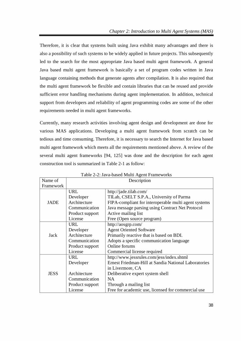
Chapter 2: Introduction to Multi Agent Systems (MAS)
38
Therefore, it is clear that systems built using Java exhibit many advantages and there is
also a possibility of such systems to be widely applied in future projects. This subsequently
led to the search for the most appropriate Java based multi agent framework. A general
Java based multi agent framework is basically a set of program codes written in Java
language containing methods that generate agents after compilation. It is also required that
the multi agent framework be flexible and contain libraries that can be reused and provide
sufficient error handling mechanisms during agent implementation. In addition, technical
support from developers and reliability of agent programming codes are some of the other
requirements needed in multi agent frameworks.
Currently, many research activities involving agent design and development are done for
various MAS applications. Developing a multi agent framework from scratch can be
tedious and time consuming. Therefore, it is necessary to search the Internet for Java based
multi agent framework which meets all the requirements mentioned above. A review of the
several multi agent frameworks [94, 125] was done and the description for each agent
construction tool is summarized in Table 2-1 as follow:
Table 2-2: Java-based Multi Agent Frameworks Name of Framework
Description
JADE
URL Developer Architecture Communication Product support License
http://jade.tilab.com/ TILab, CSELT S.P.A., University of Parma FIPA-compliant for interoperable multi agent systems Java message parsing using Contract Net Protocol Active mailing list Free (Open source program)
Jack
URL Developer Architecture Communication Product support License
http://aosgrp.com/ Agent Oriented Software Primarily reactive that is based on BDI. Adopts a specific communication language Online forums Commercial license required
JESS
URL Developer Architecture Communication Product support License
http://www.jessrules.com/jess/index.shtml Ernest Friedman-Hill at Sandia National Laboratories in Livermore, CA Deliberative expert system shell NA Through a mailing list Free for academic use, licensed for commercial use
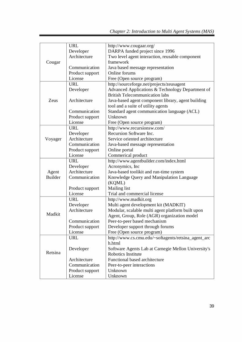
Chapter 2: Introduction to Multi Agent Systems (MAS)
39
Cougar
URL Developer Architecture Communication Product support License
http://www.cougaar.org/ DARPA funded project since 1996 Two level agent interaction, reusable component framework Java based message representation Online forums Free (Open source program)
Zeus
URL Developer Architecture Communication Product support License
http://sourceforge.net/projects/zeusagent Advanced Applications & Technology Department of British Telecommunication labs Java-based agent component library, agent building tool and a suite of utility agents Standard agent communication language (ACL) Unknown Free (Open source program)
Voyager
URL Developer Architecture Communication Product support License
http://www.recursionsw.com/ Recursion Software Inc. Service oriented architecture Java-based message representation Online portal Commerical product
Agent Builder
URL Developer Architecture Communication Product support License
http://www.agentbuilder.com/index.html Acronymics, Inc Java-based toolikit and run-time system Knowledge Query and Manipulation Language (KQML) Mailing list Trial and commercial license
Madkit
URL Developer Architecture Communication Product support License
http://www.madkit.org Multi agent development kit (MADKIT) Modular, scalable multi agent platform built upon Agent, Group, Role (AGR) organization model Peer-to-peer based mechanism Developer support through forums Free (Open source program)
Retsina
URL Developer Architecture Communication Product support License
http://www.cs.cmu.edu/~softagents/retsina_agent_arch.html Software Agents Lab at Carnegie Mellon University's Robotics Institute Functional based architecture Peer-to-peer interactions Unknown Unknown
Chapter 2: Introduction to Multi Agent Systems (MAS)
40
Among the available toolkit mentioned above, JADE was selected for this research
because it complies with the core IEEE FIPA specifications and meets all the requirements
which are necessary in implementing a normative Java based multi agent framework.
2.6.2 Java Agent Development Framework (JADE)
JADE was originally developed by Telecom Italia Lab (TILab), a R&D group which was
formerly known as Centro Studi E Laboratori Telecomunicazioni (CSELT) in Italy to
address the issue of the lack of support for developing agent based systems [117]. It is a
Java based multi agent framework and provides users with the capability to develop agent
based applications for interoperable multi agent systems which complies with IEEE FIPA
specifications. The intention of JADE is to simplify the development process while making
sure it adheres to standard compliance through an extensive set of system services and
agents. Furthermore, JADE exhibits numerous inherent features found in distributed
systems. Most of JADE's complexities are hidden from users enabling more focus on
logical aspects of the system. This allows users to zoom straight into solving problems
without having to fully understand how JADE operates internally such as agent transport,
encoding, parsing and agent life-cycle. In addition, JADE provides a runtime agent
environment, a requirement for agents to operate, a graphical interface to monitor agents as
well as an extensive library of classes with methods based on FIPA standards. JADE also
utilizes object oriented abstractions to develop FIPA-compliant agent applications and can
provide a convenient distributed platform which is suitable for microgrid control and
monitoring operations.
JADE can be illustrated as a distributed platform consisting of a main and several
peripheral containers as shown in Figure 2-7. Each container is an instance of the runtime
environment by JADE. Whenever a new agent platform is created, the main container
comprising AMS and DF agents will have to be initialized first. This is in accordance to
one of the specifications stated by FIPA. Once the main container has been initialized,
peripheral containers containing user-defined customized agents can subsequently be
created on client computers which are connected to the same network. If another agent
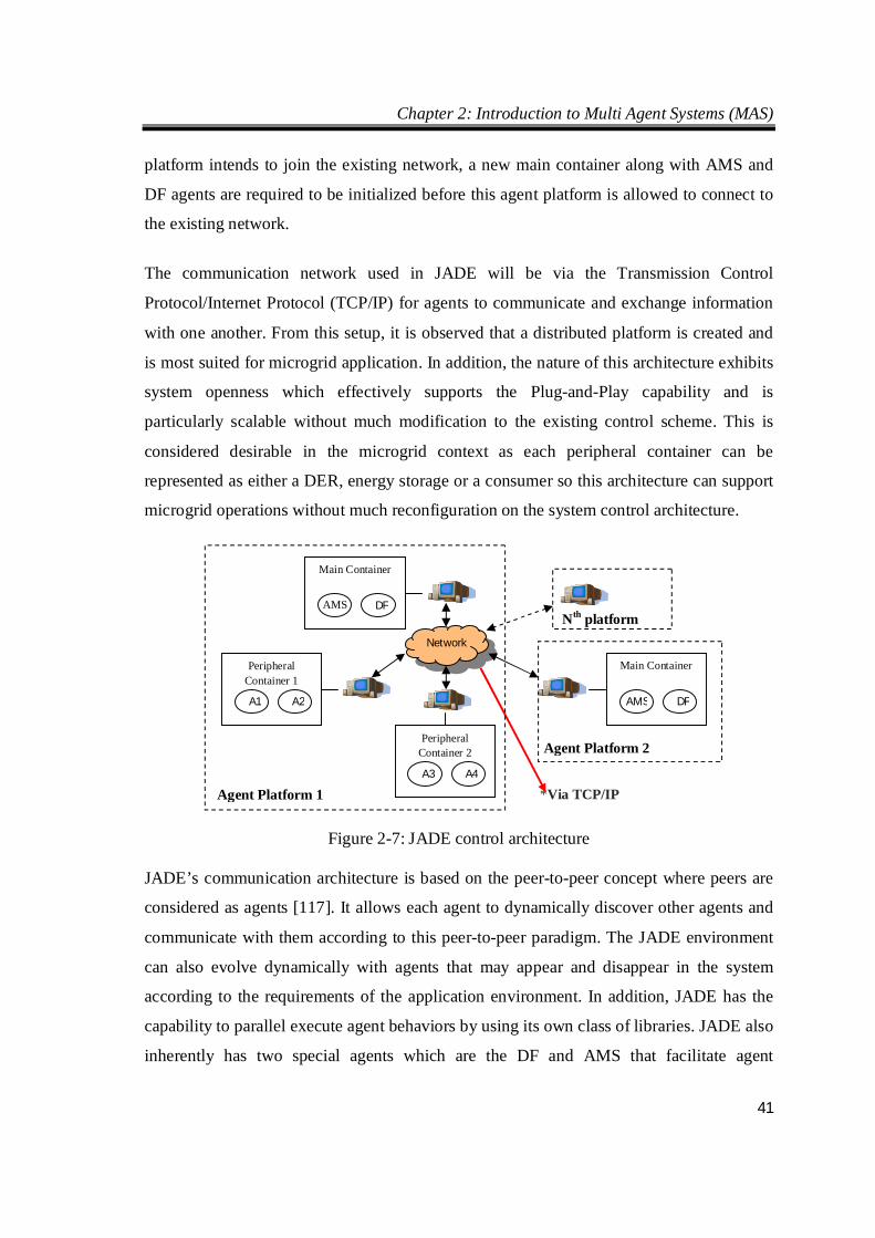
Chapter 2: Introduction to Multi Agent Systems (MAS)
41
platform intends to join the existing network, a new main container along with AMS and
DF agents are required to be initialized before this agent platform is allowed to connect to
the existing network.
The communication network used in JADE will be via the Transmission Control
Protocol/Internet Protocol (TCP/IP) for agents to communicate and exchange information
with one another. From this setup, it is observed that a distributed platform is created and
is most suited for microgrid application. In addition, the nature of this architecture exhibits
system openness which effectively supports the Plug-and-Play capability and is
particularly scalable without much modification to the existing control scheme. This is
considered desirable in the microgrid context as each peripheral container can be
represented as either a DER, energy storage or a consumer so this architecture can support
microgrid operations without much reconfiguration on the system control architecture.
Figure 2-7: JADE control architecture
JADE’s communication architecture is based on the peer-to-peer concept where peers are
considered as agents [117]. It allows each agent to dynamically discover other agents and
communicate with them according to this peer-to-peer paradigm. The JADE environment
can also evolve dynamically with agents that may appear and disappear in the system
according to the requirements of the application environment. In addition, JADE has the
capability to parallel execute agent behaviors by using its own class of libraries. JADE also
inherently has two special agents which are the DF and AMS that facilitate agent
*Via TCP/IP
Peripheral Container 1
A1 A2
Peripheral Container 2
A3 A4
Network
Agent Platform 1
Agent Platform 2
Nth platform
Main Container
DF AMS
Main Container
DF AMS
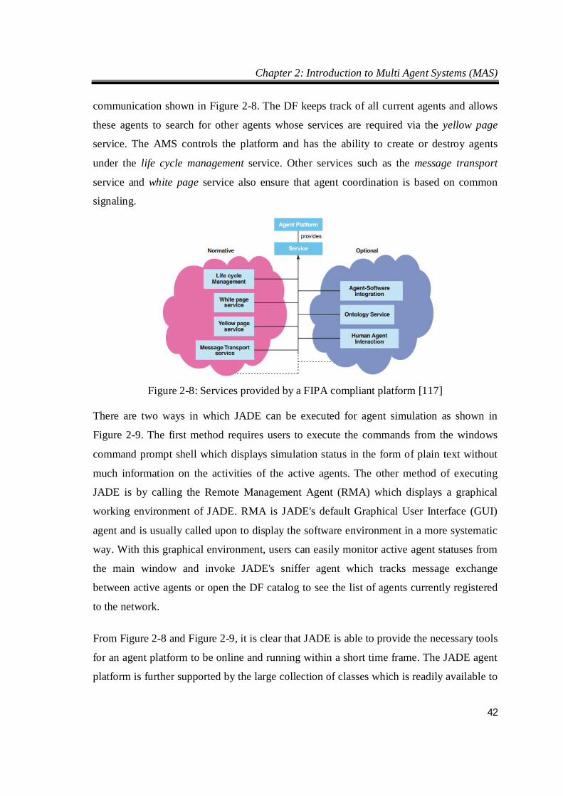
Chapter 2: Introduction to Multi Agent Systems (MAS)
42
communication shown in Figure 2-8. The DF keeps track of all current agents and allows
these agents to search for other agents whose services are required via the yellow page
service. The AMS controls the platform and has the ability to create or destroy agents
under the life cycle management service. Other services such as the message transport
service and white page service also ensure that agent coordination is based on common
signaling.
Figure 2-8: Services provided by a FIPA compliant platform [117]
There are two ways in which JADE can be executed for agent simulation as shown in
Figure 2-9. The first method requires users to execute the commands from the windows
command prompt shell which displays simulation status in the form of plain text without
much information on the activities of the active agents. The other method of executing
JADE is by calling the Remote Management Agent (RMA) which displays a graphical
working environment of JADE. RMA is JADE's default Graphical User Interface (GUI)
agent and is usually called upon to display the software environment in a more systematic
way. With this graphical environment, users can easily monitor active agent statuses from
the main window and invoke JADE's sniffer agent which tracks message exchange
between active agents or open the DF catalog to see the list of agents currently registered
to the network.
From Figure 2-8 and Figure 2-9, it is clear that JADE is able to provide the necessary tools
for an agent platform to be online and running within a short time frame. The JADE agent
platform is further supported by the large collection of classes which is readily available to
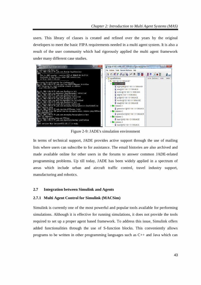
Chapter 2: Introduction to Multi Agent Systems (MAS)
43
users. This library of classes is created and refined over the years by the original
developers to meet the basic FIPA requirements needed in a multi agent system. It is also a
result of the user community which had rigorously applied the multi agent framework
under many different case studies.
Figure 2-9: JADE's simulation environment
In terms of technical support, JADE provides active support through the use of mailing
lists where users can subscribe to for assistance. The email histories are also archived and
made available online for other users in the forums to answer common JADE-related
programming problems. Up till today, JADE has been widely applied in a spectrum of
areas which include urban and aircraft traffic control, travel industry support,
manufacturing and robotics.
2.7 Integration between Simulink and Agents
2.7.1 Multi Agent Control for Simulink (MACSim)
Simulink is currently one of the most powerful and popular tools available for performing
simulations. Although it is effective for running simulations, it does not provide the tools
required to set up a proper agent based framework. To address this issue, Simulink offers
added functionalities through the use of S-function blocks. This conveniently allows
programs to be written in other programming languages such as C++ and Java which can
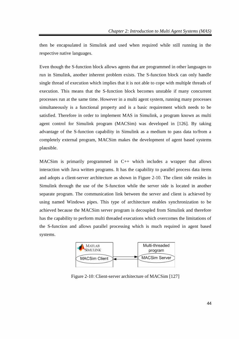
Chapter 2: Introduction to Multi Agent Systems (MAS)
44
then be encapsulated in Simulink and used when required while still running in the
respective native languages.
Even though the S-function block allows agents that are programmed in other languages to
run in Simulink, another inherent problem exists. The S-function block can only handle
single thread of execution which implies that it is not able to cope with multiple threads of
execution. This means that the S-function block becomes unstable if many concurrent
processes run at the same time. However in a multi agent system, running many processes
simultaneously is a functional property and is a basic requirement which needs to be
satisfied. Therefore in order to implement MAS in Simulink, a program known as multi
agent control for Simulink program (MACSim) was developed in [126]. By taking
advantage of the S-function capability in Simulink as a medium to pass data to/from a
completely external program, MACSim makes the development of agent based systems
plausible.
MACSim is primarily programmed in C++ which includes a wrapper that allows
interaction with Java written programs. It has the capability to parallel process data items
and adopts a client-server architecture as shown in Figure 2-10. The client side resides in
Simulink through the use of the S-function while the server side is located in another
separate program. The communication link between the server and client is achieved by
using named Windows pipes. This type of architecture enables synchronization to be
achieved because the MACSim server program is decoupled from Simulink and therefore
has the capability to perform multi threaded executions which overcomes the limitations of
the S-function and allows parallel processing which is much required in agent based
systems.
Figure 2-10: Client-server architecture of MACSim [127]
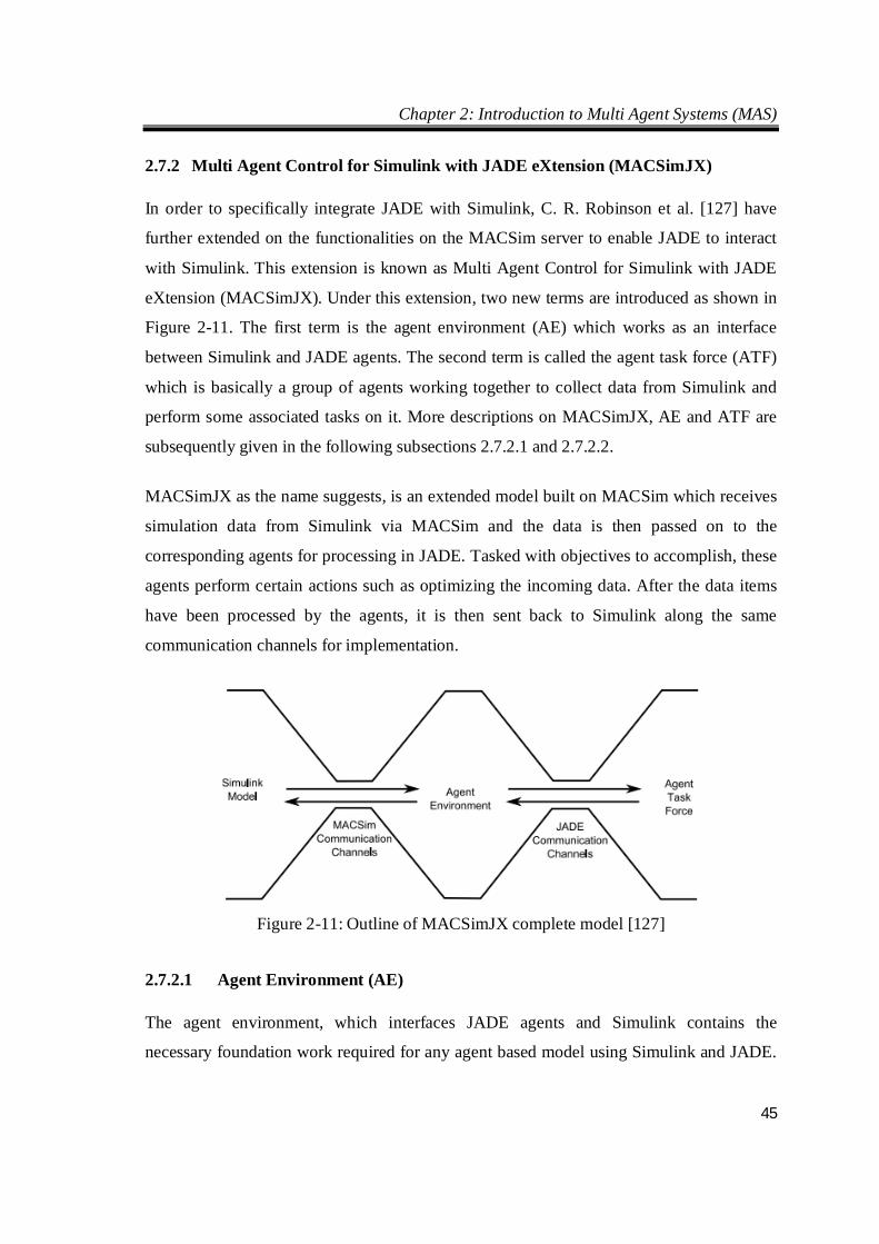
Chapter 2: Introduction to Multi Agent Systems (MAS)
45
2.7.2 Multi Agent Control for Simulink with JADE eXtension (MACSimJX)
In order to specifically integrate JADE with Simulink, C. R. Robinson et al. [127] have
further extended on the functionalities on the MACSim server to enable JADE to interact
with Simulink. This extension is known as Multi Agent Control for Simulink with JADE
eXtension (MACSimJX). Under this extension, two new terms are introduced as shown in
Figure 2-11. The first term is the agent environment (AE) which works as an interface
between Simulink and JADE agents. The second term is called the agent task force (ATF)
which is basically a group of agents working together to collect data from Simulink and
perform some associated tasks on it. More descriptions on MACSimJX, AE and ATF are
subsequently given in the following subsections 2.7.2.1 and 2.7.2.2.
MACSimJX as the name suggests, is an extended model built on MACSim which receives
simulation data from Simulink via MACSim and the data is then passed on to the
corresponding agents for processing in JADE. Tasked with objectives to accomplish, these
agents perform certain actions such as optimizing the incoming data. After the data items
have been processed by the agents, it is then sent back to Simulink along the same
communication channels for implementation.
Figure 2-11: Outline of MACSimJX complete model [127]
2.7.2.1 Agent Environment (AE)
The agent environment, which interfaces JADE agents and Simulink contains the
necessary foundation work required for any agent based model using Simulink and JADE.
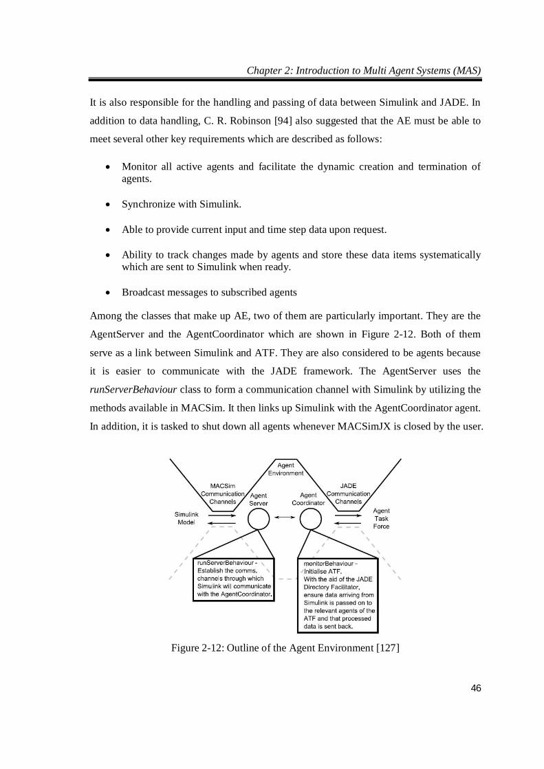
Chapter 2: Introduction to Multi Agent Systems (MAS)
46
It is also responsible for the handling and passing of data between Simulink and JADE. In
addition to data handling, C. R. Robinson [94] also suggested that the AE must be able to
meet several other key requirements which are described as follows:
Monitor all active agents and facilitate the dynamic creation and termination of agents.
Synchronize with Simulink.
Able to provide current input and time step data upon request.
Ability to track changes made by agents and store these data items systematically
which are sent to Simulink when ready.
Broadcast messages to subscribed agents Among the classes that make up AE, two of them are particularly important. They are the
AgentServer and the AgentCoordinator which are shown in Figure 2-12. Both of them
serve as a link between Simulink and ATF. They are also considered to be agents because
it is easier to communicate with the JADE framework. The AgentServer uses the
runServerBehaviour class to form a communication channel with Simulink by utilizing the
methods available in MACSim. It then links up Simulink with the AgentCoordinator agent.
In addition, it is tasked to shut down all agents whenever MACSimJX is closed by the user.
Figure 2-12: Outline of the Agent Environment [127]
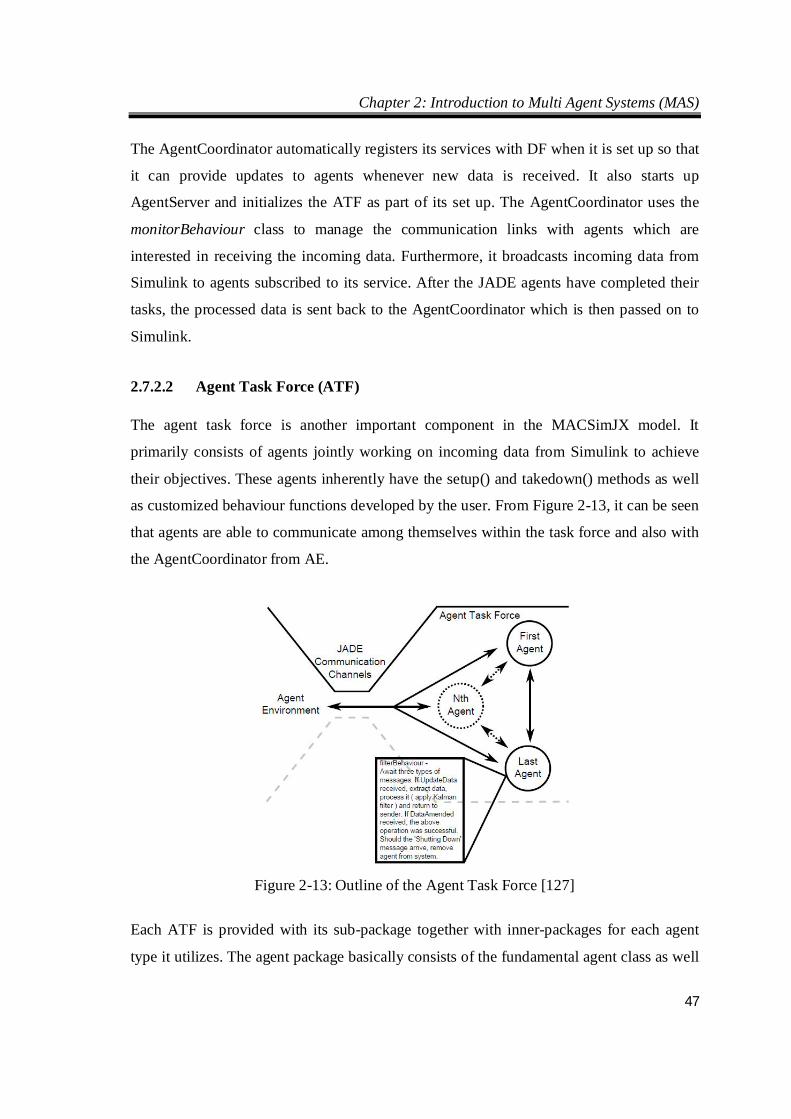
Chapter 2: Introduction to Multi Agent Systems (MAS)
47
The AgentCoordinator automatically registers its services with DF when it is set up so that
it can provide updates to agents whenever new data is received. It also starts up
AgentServer and initializes the ATF as part of its set up. The AgentCoordinator uses the
monitorBehaviour class to manage the communication links with agents which are
interested in receiving the incoming data. Furthermore, it broadcasts incoming data from
Simulink to agents subscribed to its service. After the JADE agents have completed their
tasks, the processed data is sent back to the AgentCoordinator which is then passed on to
Simulink.
2.7.2.2 Agent Task Force (ATF)
The agent task force is another important component in the MACSimJX model. It
primarily consists of agents jointly working on incoming data from Simulink to achieve
their objectives. These agents inherently have the setup() and takedown() methods as well
as customized behaviour functions developed by the user. From Figure 2-13, it can be seen
that agents are able to communicate among themselves within the task force and also with
the AgentCoordinator from AE.
Figure 2-13: Outline of the Agent Task Force [127]
Each ATF is provided with its sub-package together with inner-packages for each agent
type it utilizes. The agent package basically consists of the fundamental agent class as well
Chapter 2: Introduction to Multi Agent Systems (MAS)
48
as the associated classes to complement it. Agents residing in the ATF are created by the
AgentCoordinator. These agents have all the basic classes and methods required to operate
and can be found in a typical agent template. The only difference that differentiates ATF
agents from other agents is in the design of agent behaviours. ATF agents are designed to
look out for three message types from the AgentCoordinator and they are listed as follows:
UpdateData – Whenever an ACL message whose message ID containing the
UpdateData parameter is broadcasted by the AgentCoordinator and it is received by
the ATF agents, they will extract the data from the message content and process the
extracted data. After processing the extracted data, a reply message is generated
with message ID containing the ProcessedData parameter and message content
containing the extracted data that will be sent to the AgentCoordinator.
DataAmended – Whenever the AgentCoordinator receives messages whose
message ID contains the ProcessedData parameter, the ATF agent will generate a
reply message back to the message sender with message ID containing the
DataAmended parameter and the message content stating a confirmation of data
amended has been updated in its records. This process ends the message exchange
sequence between the AgentCoordinator and ATF agents and the entire process
will repeat when new data is received from Simulink.
Shutting Down – Each agent receiving an ACL message with message ID
containing the Shutting Down parameter is instructed to run its takedown() method
and terminate themselves by deregistering and removing all its services from the
DF. This usually occurs when the program is shut down by the user.
The three message types described above are usually the basic interactions between the
AgentCoordinator and ATF agents. Furthermore, users may also introduce additional
communication mechanisms to customize the way agents interact within the ATF and
provide another degree of freedom to the users. In this thesis, ATF agents have been
programmed to use the three basic message types mentioned above and also custom
message types to interact with JADE agents for managing the coordinated market
operation and implementation of the microgrid.
Chapter 3: Agent Design and Implementation for Proposed Microgrid Energy Market
49
CHAPTER 3 PRELIMINARY AGENT DESIGN FOR
MICROGRID MARKET OPERATION
3.1 Introduction
The first step for microgrids to effectively participate in the upstream or national energy
market is to create a local energy market. Several types of market clearing mechanisms for
microgrids have been previously proposed [97, 128-131]. For example in [129], a local
market structure has been proposed to manage the market clearing mechanism for
microgrid energy. The purchase and sale of energy in the microgrid electricity market is
basically dependent on the supply and demand in the microgrid. In addition, the supply and
demand of the microgrid are also used in setting the energy prices which is the MCP. Since
the primary objective for introducing a microgrid electricity market is to reduce electricity
prices, the energy prices determined from the microgrid's supply and demand should be
lower than the utility grid selling price for the microgrid to benefit from such a market
scheme.
In a typical electricity market, there are basically two options of bidding by generation
bidders. They are described [129] as follows:
Block generation bidding - In this bidding option, the amount of load demand
awarded to generation bidders depend on several factors which include production
cost estimates, variations in demand level, unit commitment costs and other
economic considerations.
Sealed bid auction - In this bidding option, generation bidders submit their bids to a
pool operator to procure a certain amount of load which is forecasted by the pool
operator. The objective of each generation bidder is to maximize its own benefits
while the pool operator adopts a dispatch strategy which maximizes consumer
welfare.
In addition, there are two general market clearing rules commonly used in real-time
electricity markets and they are described as follows:

Chapter 3: Agent Design and Implementation for Proposed Microgrid Energy Market
50
Uniform/Single price – This rule is commonly applied in today’s electricity
markets. During market clearing, energy sellers will be paid for the sale of
electricity based on MCP, regardless of whether they bid higher or lower than MCP.
Similarly, energy buyers will pay for the purchase of electricity at MCP, regardless
of whether they bid higher or lower than MCP. As a result, all bids to buy/sell
energy will be priced at the marginal cost of the electricity.
Discriminatory/Pay-as-bid – In this rule, energy sellers with the winning bid will be
paid at their bid price. Similarly, energy buyers with the winning bid will pay at
their bid price. In this process, every participant bids by guessing the cut-off price
which is done by monitoring the market clearing results of the hourly bids over a
24-h period. However, this rule has a major drawback i.e. incorrect guessing of the
cut-off price may result in increased cost that is above MCP. This may lead to a
less efficient market clearing system which may not be desirable.
Based on the two market clearing rules mentioned above, S. Chowdhury [129] claimed that
the uniform/single price rule is most suited for restructured electricity markets because it is
believed that such a pricing rule will encourage participants to reveal their true cost which
is beneficial to every participant. This will lead to a more efficient system which is
desirable in the long run.
There are also two types of bidding mechanisms used in electricity markets i.e. the single
side and double side bidding which are shown in Figure 3-1. The main difference between
the two bidding procedures is the participation of consumers during the bidding process as
well as the price elasticity of consumers. In single side bidding, generating units are
allowed to participate in the energy market while consumers do not participate in the
energy market and are considered to be fixed loads which need to be served regardless of
market price. For double side bidding, both the generation as well as the consumer load
participate in the energy trading market and are responsive to market price actions. In
addition, generating units do not have any information on the current level of demand and
consumers do not know the availability of energy in the microgrid. In both bidding
mechanisms, it is generally considered that the generating units consist of Combined Heat
and Power (CHP) units, renewable energy sources and diesel generators. It should be noted
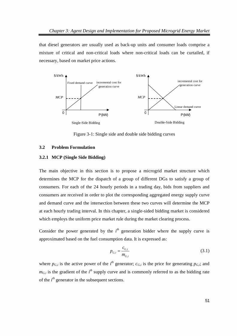
Chapter 3: Agent Design and Implementation for Proposed Microgrid Energy Market
51
that diesel generators are usually used as back-up units and consumer loads comprise a
mixture of critical and non-critical loads where non-critical loads can be curtailed, if
necessary, based on market price actions.
Figure 3-1: Single side and double side bidding curves
3.2 Problem Formulation
3.2.1 MCP (Single Side Bidding)
The main objective in this section is to propose a microgrid market structure which
determines the MCP for the dispatch of a group of different DGs to satisfy a group of
consumers. For each of the 24 hourly periods in a trading day, bids from suppliers and
consumers are received in order to plot the corresponding aggregated energy supply curve
and demand curve and the intersection between these two curves will determine the MCP
at each hourly trading interval. In this chapter, a single-sided bidding market is considered
which employs the uniform price market rule during the market clearing process.
Consider the power generated by the ith generation bidder where the supply curve is
approximated based on the fuel consumption data. It is expressed as:
,,
,
G iG i
G i
cp
m (3.1)
where pG,i is the active power of the ith generator; cG,i is the price for generating pG,i; and
mG,i is the gradient of the ith supply curve and is commonly referred to as the bidding rate
of the ith generator in the subsequent sections.
P (kW)
$/kWh
0
MCP
incremental cost for generation curve
Fixed demand curve
Single-Side Bidding Double-Side Bidding
P (kW)
$/kWh
0
MCP
incremental cost for generation curve
Linear demand curve
Chapter 3: Agent Design and Implementation for Proposed Microgrid Energy Market
52
Next, the total supply curve for N generation bidders can be found and is given as:
, ,1 ,2 ,
,1 ,2 ,
,1 ,2 ,
,
1 ,
G Total G G G N
G G G N
G G G N
NG i
i G i
p p p pc c cm m m
cm
(3.2)
Since the load demand is considered to be constant in a single side bidding market, the
total load demand in this case is denoted by D. At MCP, the common price is denoted as
cMCP and the total generation must be equal to the total load demand which is given as
follows:
1 ,
1N
MCPi G i
c Dm
(3.3)
By rearranging and making cMCP as the subject, the value of cMCP can be found as given:
1 ,
1MCP N
i G i
Dc
m
(3.4)
The equation provided in (3.4) assumes that generation bidders have sufficient capacity for
generation. If minimum and maximum generation capacity limits denoted by pG,i,min and
pG,i,,max are considered, then the total supply curve for N generation bidders is given as:
,, , , ,min , ,max
1 ,
NG i
G Total G i G i G G ii G i
cp U p p U p p
m
(3.5)
where,
, , ,min, , ,min
, , ,min
1, when 0, when
G i G iG i G i
G i G i
p pU p p
p p
, , ,max, , ,max
, , ,max
1, when 0, when
G i G iG i G i
G i G i
p pU p p
p p
By equating (3.5) with D, the updated value of cMCP can be found and is given as:
, , ,min , , ,max
1 ,
1MCP N
G i G i G i G ii G i
DcU p p U p p
m
(3.6)
Chapter 3: Agent Design and Implementation for Proposed Microgrid Energy Market
53
Hence, the MCP at each hourly trading interval is determined by (3.4). In the simulation
study later on, a Price Agent (PA) was developed which employs the MCP algorithm
presented earlier. The algorithm requests each Generation Agent (GA) and each Load
Agent (LA) for the bidding rates of generation and demand curves respectively. Once MCP
is computed, trading between the GA and LA can proceed for the current trading interval.
3.2.2 Cooperative and Competitive Pricing Strategy
In [85], I. Zabet and M. Montazeri discuss cooperative and competitive strategies for
decentralized agent control. In the context of microgrids, a cooperative strategy aims at
maximizing the benefits for the entire microgrid. This means that generation and load
agents within the microgrid network will attempt to negotiate and satisfy the local
microgrid load demand before importing/exporting power from the utility grid. As a result,
minimal power will be bought from the utility grid since load demand is prioritized to be
satisfied internally first before asking the utility grid for extra power. Thus, this
arrangement reduces the amount of power bought from the utility grid. In terms of DER's
energy pricing, Figure 3-2 shows that when the MCP obtained from (3.4) is below the
utility grid's selling price, consumers will enjoy the lower costs of purchasing energy from
the DGs within the microgrid. However, this strategy does not maximize the profit for the
DGs because their main priority is to satisfy the microgrid internal load before selling any
excess power back to the utility grid. The MCP in this strategy may fall below the grid's
buyback price so this is why cooperative strategy does not yield a maximized profit for
DGs.
In a competitive strategy, the objective of generation agents is to maximize profit for the
DGs in the microgrid. Instead of satisfying local load demand, DGs are pricing their
energy competitively with the utility grid's selling and buyback price in order to maximize
their profit. This means that DGs will not prioritize local load demand as their main
priority and any shortfall in unsatisfied load demand will be met by the utility grid. In
terms of DG pricing, Figure 3-2 shows the acceptable range of MCP for competitive
pricing which falls in between the grid's selling and grid's buyback prices. The reason for
not permitting MCP to fall below the grid’s buyback price is because in the event MCP
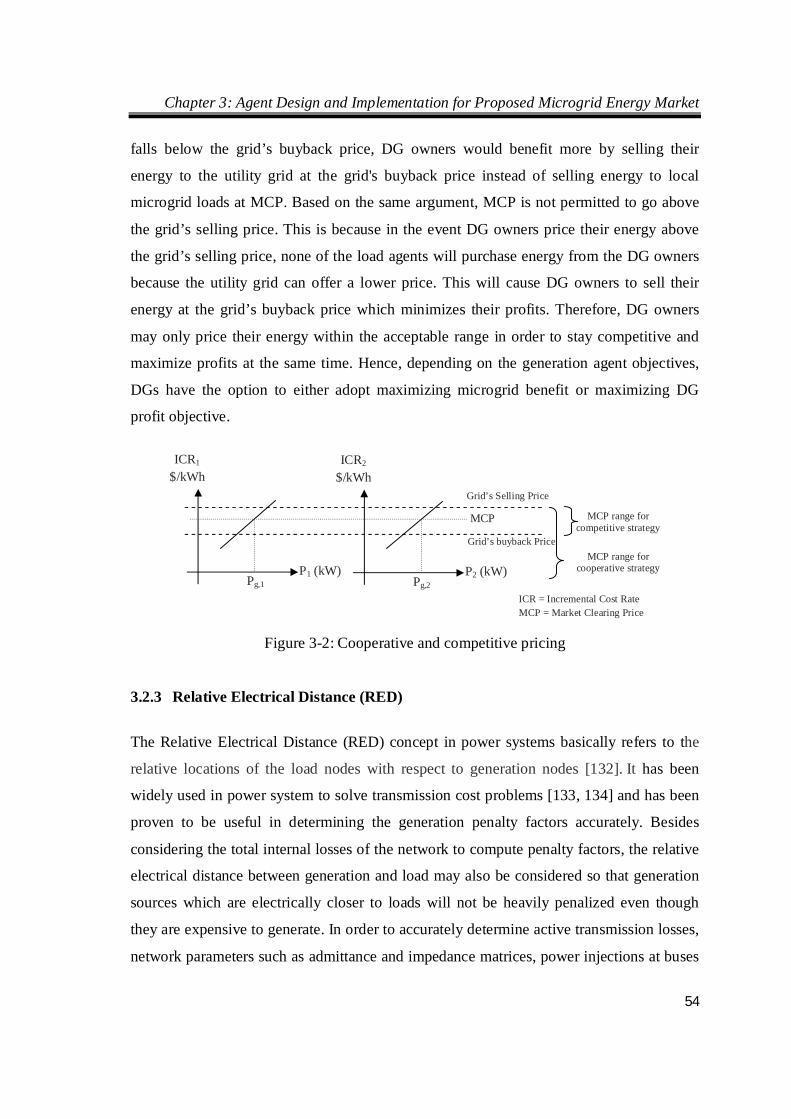
Chapter 3: Agent Design and Implementation for Proposed Microgrid Energy Market
54
falls below the grid’s buyback price, DG owners would benefit more by selling their
energy to the utility grid at the grid's buyback price instead of selling energy to local
microgrid loads at MCP. Based on the same argument, MCP is not permitted to go above
the grid’s selling price. This is because in the event DG owners price their energy above
the grid’s selling price, none of the load agents will purchase energy from the DG owners
because the utility grid can offer a lower price. This will cause DG owners to sell their
energy at the grid’s buyback price which minimizes their profits. Therefore, DG owners
may only price their energy within the acceptable range in order to stay competitive and
maximize profits at the same time. Hence, depending on the generation agent objectives,
DGs have the option to either adopt maximizing microgrid benefit or maximizing DG
profit objective.
Figure 3-2: Cooperative and competitive pricing 3.2.3 Relative Electrical Distance (RED)
The Relative Electrical Distance (RED) concept in power systems basically refers to the
relative locations of the load nodes with respect to generation nodes [132]. It has been
widely used in power system to solve transmission cost problems [133, 134] and has been
proven to be useful in determining the generation penalty factors accurately. Besides
considering the total internal losses of the network to compute penalty factors, the relative
electrical distance between generation and load may also be considered so that generation
sources which are electrically closer to loads will not be heavily penalized even though
they are expensive to generate. In order to accurately determine active transmission losses,
network parameters such as admittance and impedance matrices, power injections at buses
P1 (kW)
ICR1
$/kWh
P2 (kW)
ICR2
$/kWh
Grid’s Selling Price
Grid’s buyback Price
MCP range for competitive strategy
MCP range for cooperative strategy
Pg,1 Pg,2
MCP
ICR = Incremental Cost Rate MCP = Market Clearing Price
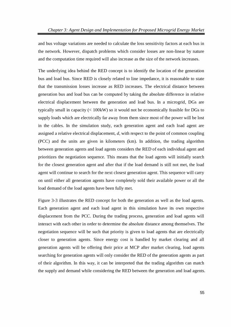
Chapter 3: Agent Design and Implementation for Proposed Microgrid Energy Market
55
and bus voltage variations are needed to calculate the loss sensitivity factors at each bus in
the network. However, dispatch problems which consider losses are non-linear by nature
and the computation time required will also increase as the size of the network increases.
The underlying idea behind the RED concept is to identify the location of the generation
bus and load bus. Since RED is closely related to line impedance, it is reasonable to state
that the transmission losses increase as RED increases. The electrical distance between
generation bus and load bus can be computed by taking the absolute difference in relative
electrical displacement between the generation and load bus. In a microgrid, DGs are
typically small in capacity (< 100kW) so it would not be economically feasible for DGs to
supply loads which are electrically far away from them since most of the power will be lost
in the cables. In the simulation study, each generation agent and each load agent are
assigned a relative electrical displacement, d, with respect to the point of common coupling
(PCC) and the units are given in kilometers (km). In addition, the trading algorithm
between generation agents and load agents considers the RED of each individual agent and
prioritizes the negotiation sequence. This means that the load agents will initially search
for the closest generation agent and after that if the load demand is still not met, the load
agent will continue to search for the next closest generation agent. This sequence will carry
on until either all generation agents have completely sold their available power or all the
load demand of the load agents have been fully met. Figure 3-3 illustrates the RED concept for both the generation as well as the load agents.
Each generation agent and each load agent in this simulation have its own respective
displacement from the PCC. During the trading process, generation and load agents will
interact with each other in order to determine the absolute distance among themselves. The
negotiation sequence will be such that priority is given to load agents that are electrically
closer to generation agents. Since energy cost is handled by market clearing and all
generation agents will be offering their price at MCP after market clearing, load agents
searching for generation agents will only consider the RED of the generation agents as part
of their algorithm. In this way, it can be interpreted that the trading algorithm can match
the supply and demand while considering the RED between the generation and load agents.
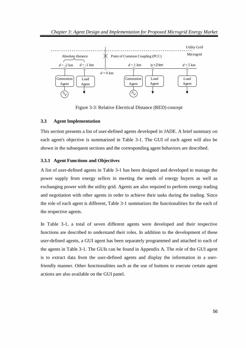
Chapter 3: Agent Design and Implementation for Proposed Microgrid Energy Market
56
Figure 3-3: Relative Electrical Distance (RED) concept
3.3 Agent Implementation
This section presents a list of user-defined agents developed in JADE. A brief summary on
each agent's objective is summarized in Table 3-1. The GUI of each agent will also be
shown in the subsequent sections and the corresponding agent behaviors are described.
3.3.1 Agent Functions and Objectives
A list of user-defined agents in Table 3-1 has been designed and developed to manage the
power supply from energy sellers in meeting the needs of energy buyers as well as
exchanging power with the utility grid. Agents are also required to perform energy trading
and negotiation with other agents in order to achieve their tasks during the trading. Since
the role of each agent is different, Table 3-1 summarizes the functionalities for the each of
the respective agents.
In Table 3-1, a total of seven different agents were developed and their respective
functions are described to understand their roles. In addition to the development of these
user-defined agents, a GUI agent has been separately programmed and attached to each of
the agents in Table 3-1. The GUIs can be found in Appendix A. The role of the GUI agent
is to extract data from the user-defined agents and display the information in a user-
friendly manner. Other functionalities such as the use of buttons to execute certain agent
actions are also available on the GUI panel.
Generation Agent
Generation Agent
Load Agent
Load Agent
Load Agent
Point of Common Coupling (PCC) Microgrid
Utility Grid
d = 1 km d = 2 km d = 5 km d = -2 km d = -1 km
Absolute distance
d = 0 km
Chapter 3: Agent Design and Implementation for Proposed Microgrid Energy Market
57
Table 3-1: List of user-defined agent functions
Agent Functions Generation Agent (GA)
Collects information on DG's power setting, MCP, electrical distance from PCC, bidding rates and DG owner's objective to participate in the energy trading
Load Agent (LA)
Captures information on consumer load demands, electrical distance of the loads from PCC and MCP. It represents consumer loads to participate in the purchase of energy during the
trading process Monitor
Agent (MA) Requests status updates from GA and LA which are then displayed via the GUI
Grid Agent (GrA)
Collects information on the grid's energy prices which are then broadcasted to inform all other agents
Price Agent (PA)
Requests bidding rates from GA and LA. MCP is computed and broadcasted to GA, LA and CA
Aggregate Agent (AA)
Requests information from GA and LA. It then computes the microgrid’s total and current available generation as well as total load demand and satisfied load
Control Agent (CA)
Captures information such as MCP, grid energy prices, total generation and load demand as well as net power exchange with GrA. It also initiates the beginning and the end of the
trading session and performs a reset on all agents in preparation for the next trading hour In addition to the functionalities described, two agent objectives are also defined for
simulation study. The first objective is defined as the maximization of load benefits where
agents will aim at minimizing the load costs of LAs. This means that the LAs will try to
negotiate with either the GAs or the utility grid to obtain the lowest offer for satisfying its
load demand. The second objective is defined as the profit maximization of GAs where
agents aim at maximizing the revenue and profit of GAs. This means that GAs will try to
negotiate with either the LAs or the utility grid to obtain the highest offer for selling its
power. It also implies that if the utility grid buyback price is higher than the LA’s offer,
GAs will sell their power to the utility grid and the LAs will have to buy from the utility
grid for that particular period. Therefore, depending on the agent’s objectives the amount
of revenue/profit received by GAs and the amount paid by LAs will vary. The results are
discussed in Section 3.4.
3.3.2 Generation Agent
The primary function of the Generation Agent (GA) is to collect information from the DG
owners and use the data to participate in the local microgrid energy market by
communicating with other participating agents. Figure A-1 in Appendix A shows the GUI
of a GA where certain parameters such as available power, incremental cost, electrical
Chapter 3: Agent Design and Implementation for Proposed Microgrid Energy Market
58
distance from PCC, and agent objective are to be filled in by the DG owner. Other
parameters such as agent identifier, grid prices, microgrid operating mode and MCP are
automatically displayed on the GUI panel upon updating the GUI.
The lists of behaviors associated with Generation Agent (GA) are described as follows:
Receive grid's energy prices behavior - This behavior is classified as cyclic and it
constantly checks for messages sent from Grid Agent (GrA). Incoming messages
received by this behavior inform GA on the grid's selling and buying energy prices
which are shown on the GUI.
Send bidding data and receive MCP behavior - This behavior is cyclic and
constantly checks for messages sent from Price Agent (PA). This behavior targets
two types of messages. The first type requests GAs to provide their bidding rate
data to PA for computing the MCP value. After the MCP is calculated by PA, the
second type of message is sent to GAs informing them on the current MCP value.
Based on the GA's objective, it will then decide whether to sell its energy at MCP
or at the grid's buying price.
End current trading session behavior - This behavior is cyclic and constantly checks
for two types of messages sent from Control Agent (CA). The first type of message
is to receive the end trading signal from CA. Once this message is received, GA
will settle any outstanding power by selling it back to GrA during grid connected
mode of operation. The second type of message from CA is to inform GA that the
current trading session is closed and it requests GA to reset its current database in
preparation for the next trading session.
Send status behavior - This behavior is cyclic and constantly checks for request
messages from Monitor Agent (MA). Upon receiving the message from MA, the
GA will create a reply message stating its current total and available power
generation as well as its current bidding rate data.
Send total and available generation behavior - This behavior is cyclic and
constantly checks for messages from AA. Upon receiving the request message
from AA, the GA will create a reply message stating its total generation and
remaining available generation status to AA.
Chapter 3: Agent Design and Implementation for Proposed Microgrid Energy Market
59
Trading behavior - This behavior is cyclic and constantly checks for messages from
Load Agent (LA). Upon receiving message requests from LAs, this behavior will
first check the electrical distance between itself and LA. Secondly, this behavior
will check whether it has sufficient generation to satisfy LA. If GA has insufficient
generation, it will only supply whatever remaining generation to LA and request
LA to search for other sources to satisfy its total load demand. Finally, this
behavior executes the transaction between GA and LA on the energy settlement and
update GA's remaining available generation for other subsequent LA’s requests.
3.3.3 Load Agent
This agent represents consumers to participate in the local microgrid energy market to
purchase energy. Figure A-2 in Appendix A illustrates the GUI of a Load Agent (LA)
where the input parameters include load demand and electrical distance from PCC. Other
parameters such as LA buying status, grid prices, load status and microgrid operating mode
are automatically updated on the GUI upon refreshing.
The list of behaviors associated with this agent is described as follows:
Receive grid price and microgrid status behavior - This behavior is cyclic and
constantly checks for messages sent from GrA. Messages received contain
information on the grid's selling price and operating mode of the microgrid.
Send load demand data and receive MCP behavior - This behavior is cyclic and
constantly checks for request messages from PA. Whenever a message is received
from PA, it will create a reply message stating its load demand data so that PA can
compute the MCP. After MCP is calculated, PA will send an inform message to LA
containing MCP data which will be updated in the LA's GUI.
Send status behavior - This behavior is cyclic and constantly checks for messages
sent from MA. Upon receiving request messages from MA, this agent will create a
reply message stating the LA's load demand level and amount of load being
purchased currently.
Chapter 3: Agent Design and Implementation for Proposed Microgrid Energy Market
60
Send total demand and satisfied load demand behavior - This behavior is cyclic and
constantly checks for request messages sent from AA. Upon receiving the request
message, this agent will send a reply message to AA stating its total load demand
and satisfied load demand to AA.
Trading behavior - This behavior is cyclic and constantly checks for messages sent
from CA. Upon receiving trading signal messages, this agent will automatically
begin the current trading session by searching for GA to purchase energy. There are
several message exchanges between LA and GA during trading. The first message
searches for the nearest available GA to supply and the second request message
checks for the next available GA if its demand is not fully satisfied by the previous
GA. Another type of message received is to inform LA that the current trading
session has ended and to request LA to settle any unsatisfied load demand with
GrA in grid connected mode. The end trading message will inform LA to reset its
current database in preparation for the next trading session.
3.3.4 Monitor Agent
This agent requests status updates from GA and LA and displays the information on its
GUI. Figure A-3 in Appendix A shows a GUI snapshot of MA. This is a basic GUI
displaying all active GAs and LAs currently participating in the trading session with their
statuses displayed beside their respective agent identifiers. Thus through this agent,
monitoring of GA and LA status can be done.
The list of behaviors associated with this agent is described as follows:
Receive GA status behavior - This behavior is cyclic and constantly checks for
messages sent by GAs. The messages contain information on every active GA
which includes its total generation and remaining available generation status as
well as its bidding rate data.
Receive LA status behavior - This behavior is cyclic and constantly checks for
messages sent by LA. The messages contain information on every LA which
includes load demand and amount of power being purchased currently.
Chapter 3: Agent Design and Implementation for Proposed Microgrid Energy Market
61
3.3.5 Grid Agent
This agent collects information on the grid's selling and buyback energy prices as well as
the microgrid operating mode. Figure A-4 in Appendix A provides a GUI snapshot of Grid
Agent (GrA). The GUI essentially collects inputs such as the grid's selling price and the
microgrid status and automatically displays the information on the GUI panel. One point to
note is that the grid's buyback price is automatically computed based on the grid's selling
price. This is because the utility grid imposes an additional surcharge when the microgrid
sells power back to the grid. Hence, the grid's buyback price is usually lower than its
selling price.
The list of behaviors associated with this agent is described as follows:
Update grid prices and microgrid status behavior - This behavior is classified as
one-shot because it waits for the GUI before executing its updating routine. Upon
receiving inputs from the GUI, this behavior will update GrA on the latest grid's
prices and microgrid operating mode which are then displayed on the GUI panel
when the Refresh button is used. It should be noted that the buttons created in the
agent’s GUI are designed to be manually triggered by the user in order to verify the
functionality of the agent at each step in the algorithm. However in practice, the
agent can be programmed to automatically execute certain actions at specific time
intervals using the cyclic behavior.
Broadcast grid prices and microgrid status behavior - This behavior is also one-shot
as it has to wait for the GUI before broadcasting its information. Upon using GUI
to update this agent, this behavior is simultaneously triggered to broadcast the
updated information to GA, LA, PA, AA and CA.
3.3.6 Price Agent
The main function of the PA is to collect the bidding information from GA and LA in
order to compute MCP for each hour trading session. Figure A-5 in Appendix A shows a
snapshot of the agent's GUI. When the Compute and Broadcast MCP button is triggered,
the agent will proceed to compute the MCP. This GUI does not require any GUI inputs to
Chapter 3: Agent Design and Implementation for Proposed Microgrid Energy Market
62
function. When MCP is computed, its value will be displayed along with other parameters
such as grid prices, microgrid operating mode and load demand.
The list of behaviors associated with this agent is described as follows:
Receive grid's prices and microgrid status behavior - This behavior is cyclic and
constantly checks for messages sent by GrA. Whenever GrA updates its selling and
buyback prices, it will send a message to inform this agent. The connection status
of the microgrid is also included into the message to inform PA on the operating
mode of the microgrid.
Compute and Broadcast MCP behavior - This behavior is one-shot because it
requires users to press the Compute and Broadcast MCP button on the GUI before
MCP can be computed. Once this behavior is triggered, it will request every GA for
its bidding rate data and every LA for its load demand data. After that, it will
compute the MCP and determine whether the MCP value is higher than the grid's
selling price. If the MCP is higher than the grid's selling price, this agent will set
MCP at the grid's selling price so that DGs can sell their energy to local consumers
instead of consumers buying energy from the grid. After MCP is computed, it will
correspondingly inform the GA, LA and CA.
3.3.7 Aggregate Agent
The main function of the AA is to consolidate all GAs and LAs in the microgrid and
display the total microgrid generation and load demand in the GUI. Figure A-6 in
Appendix A illustrates a GUI snapshot of the Aggregate Agent (AA). It requires GUI
inputs in order to function. Whenever the update button is executed, it will begin
aggregating data from the GAs and LAs and the updated data will be reflected on the GUI.
The list of behaviors associated with this agent is described as follows:
Receive grid prices behavior - This behavior is cyclic and constantly checks for
messages sent by GrA. When GrA updates its energy prices, a message will be sent
to this agent where this behavior will be responsible for decrypting the message
contents and update this agent accordingly.
Chapter 3: Agent Design and Implementation for Proposed Microgrid Energy Market
63
Receive GA status behavior - This behavior is cyclic and constantly checks for
messages sent by GAs. When request messages are sent to GAs requesting for their
generation status, GA will send a reply message to this agent where the message
will be decrypted in this behavior. Message contents include GA's rated generation
and remaining available generation. Once the generation statuses for all GAs have
been collected, this agent will aggregate the data and display it on the GUI.
Receive LA status behavior - This behavior is cyclic and constantly checks for
messages sent by LA. Whenever this agent requests for LA's demand status, LA
will send a reply message to this agent where it will be decrypted in this behavior.
The contents of the message include each LA's total load demand and satisfied load
demand data. After collecting data from all LAs, this agent aggregates the data and
displays them in the GUI.
End of current trading session and inform CA behavior - This behavior is cyclic
and constantly checks for messages sent by CA. When the end of current trading
session message is sent by CA, this behavior will receive the message and perform
an internal update to collect current GA and LA statuses. The updated information
is then sent back to CA containing all the GA and LA statuses after the current
trading session.
3.3.8 Control Agent
This agent serves as a control for the operation of energy trading between GAs and LAs as
well as recording the amount of microgrid power exchange with the utility grid. Figure A-7
in Appendix A shows a snapshot of the Control Agent (CA)'s GUI. This GUI displays
parameters such as microgrid operating mode, grid prices, MCP, microgrid generation and
load demand details. Users can press the update button on this GUI to update the microgrid
parameters which will be subsequently reflected on the GUI. The Initiate Trade button tells
this agent to start the current trading session by sending messages to GAs and LAs to
inform them. This will trigger the start of the current trading session. When all GAs and
LAs are done, the End Trade button is triggered to signal the end of the current trading
session. During this time, GAs and LAs are required to settle their generation and load
demand respectively and the final simulation results can be printed on the Windows
Chapter 3: Agent Design and Implementation for Proposed Microgrid Energy Market
64
command prompt. The Reset Simulation button is triggered to prepare GAs and LAs for
the next trading session.
The list of behaviors associated with this agent is described as follows:
Receive grid prices and microgrid status behavior - This behavior is cyclic and
constantly checks for messages sent by GrA. It looks for messages sent by GrA in
order to update this agent on the grid's energy prices. The message contents include
grid prices and microgrid operating status.
Receive MCP behavior - This behavior is cyclic and constantly checks for
messages sent by PA. After MCP is computed, PA will send a message to this
agent and this behavior is responsible for obtaining the information. The updated
MCP will be reflected in the GUI.
Receive AA data behavior - This behavior is cyclic and constantly checks for
messages sent by AA. When the Update button is triggered, it will send a request
message to AA asking for the updated information. AA will send a reply message
to this agent where it will be received by this behavior. Message contents include
microgrid total generation and load demand status. CA then computes the net
power flow from the microgrid and indicates whether a surplus or deficit in
microgrid energy has occurred during the current trading session.
Initiate trade behavior - This behavior is one-shot and is only triggered through this
GUI when the Initiate Trade button is triggered. This signifies the start of the
current trading session where it will inform all GAs and LAs to begin trading.
End trade behavior - This behavior is one-shot and is triggered through the GUI
when the End Trade button is triggered. It will send messages to all GAs and LAs
informing them to settle any outstanding generation and load demand respectively.
After which, CA will declare the end of the current trading session.
Reset simulation behavior - This behavior is one-shot and is triggered when the
Reset Simulation button is triggered. CA will send messages to all other agents
telling them to reset their database in preparation for the next trading session.
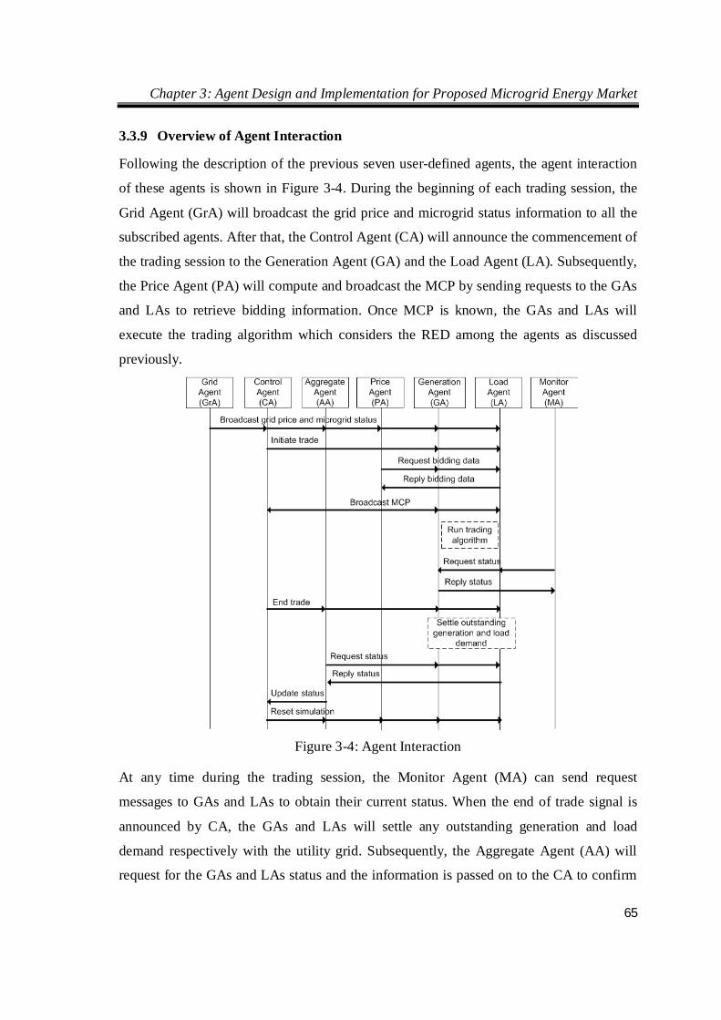
Chapter 3: Agent Design and Implementation for Proposed Microgrid Energy Market
65
3.3.9 Overview of Agent Interaction
Following the description of the previous seven user-defined agents, the agent interaction
of these agents is shown in Figure 3-4. During the beginning of each trading session, the
Grid Agent (GrA) will broadcast the grid price and microgrid status information to all the
subscribed agents. After that, the Control Agent (CA) will announce the commencement of
the trading session to the Generation Agent (GA) and the Load Agent (LA). Subsequently,
the Price Agent (PA) will compute and broadcast the MCP by sending requests to the GAs
and LAs to retrieve bidding information. Once MCP is known, the GAs and LAs will
execute the trading algorithm which considers the RED among the agents as discussed
previously.
Figure 3-4: Agent Interaction
At any time during the trading session, the Monitor Agent (MA) can send request
messages to GAs and LAs to obtain their current status. When the end of trade signal is
announced by CA, the GAs and LAs will settle any outstanding generation and load
demand respectively with the utility grid. Subsequently, the Aggregate Agent (AA) will
request for the GAs and LAs status and the information is passed on to the CA to confirm
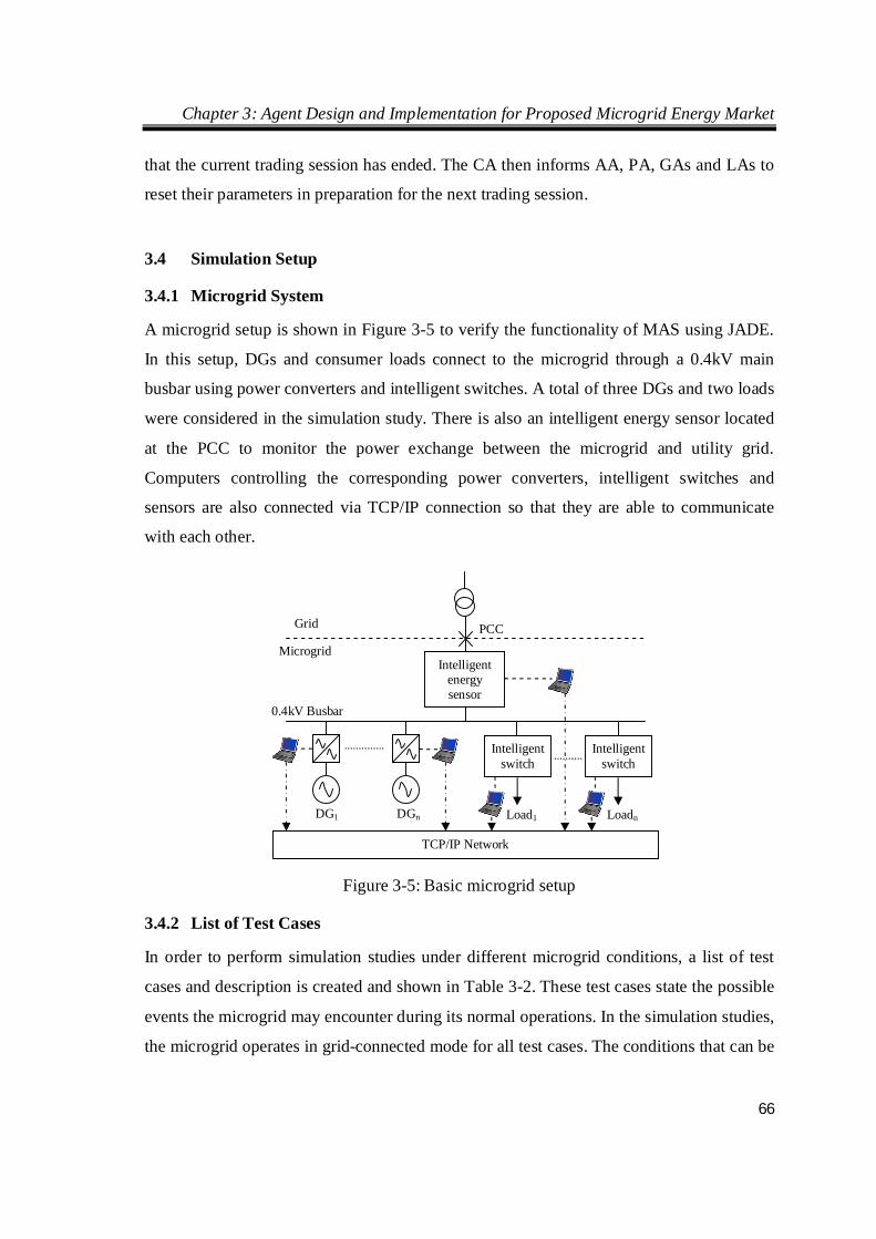
Chapter 3: Agent Design and Implementation for Proposed Microgrid Energy Market
66
that the current trading session has ended. The CA then informs AA, PA, GAs and LAs to
reset their parameters in preparation for the next trading session.
3.4 Simulation Setup
3.4.1 Microgrid System
A microgrid setup is shown in Figure 3-5 to verify the functionality of MAS using JADE.
In this setup, DGs and consumer loads connect to the microgrid through a 0.4kV main
busbar using power converters and intelligent switches. A total of three DGs and two loads
were considered in the simulation study. There is also an intelligent energy sensor located
at the PCC to monitor the power exchange between the microgrid and utility grid.
Computers controlling the corresponding power converters, intelligent switches and
sensors are also connected via TCP/IP connection so that they are able to communicate
with each other.
Figure 3-5: Basic microgrid setup
3.4.2 List of Test Cases
In order to perform simulation studies under different microgrid conditions, a list of test
cases and description is created and shown in Table 3-2. These test cases state the possible
events the microgrid may encounter during its normal operations. In the simulation studies,
the microgrid operates in grid-connected mode for all test cases. The conditions that can be
Intelligent energy sensor
Grid
Microgrid
PCC
Intelligent switch
Intelligent switch
DG1 DGn Load1 Loadn
TCP/IP Network
0.4kV Busbar
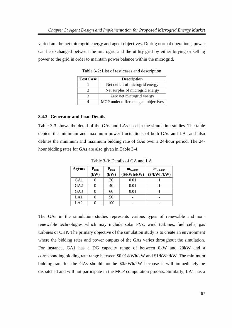
Chapter 3: Agent Design and Implementation for Proposed Microgrid Energy Market
67
varied are the net microgrid energy and agent objectives. During normal operations, power
can be exchanged between the microgrid and the utility grid by either buying or selling
power to the grid in order to maintain power balance within the microgrid.
Table 3-2: List of test cases and description
Test Case Description 1 Net deficit of microgrid energy 2 Net surplus of microgrid energy 3 Zero net microgrid energy 4 MCP under different agent objectives
3.4.3 Generator and Load Details
Table 3-3 shows the detail of the GAs and LAs used in the simulation studies. The table
depicts the minimum and maximum power fluctuations of both GAs and LAs and also
defines the minimum and maximum bidding rate of GAs over a 24-hour period. The 24-
hour bidding rates for GAs are also given in Table 3-4.
Table 3-3: Details of GA and LA
Agents Pmin (kW)
Pmax (kW)
mG,i,min ($/kWh/kW)
mG,i,max
($/kWh/kW) GA1 0 20 0.01 1 GA2 0 40 0.01 1 GA3 0 60 0.01 1 LA1 0 50 - - LA2 0 100 - -
The GAs in the simulation studies represents various types of renewable and non-
renewable technologies which may include solar PVs, wind turbines, fuel cells, gas
turbines or CHP. The primary objective of the simulation study is to create an environment
where the bidding rates and power outputs of the GAs varies throughout the simulation.
For instance, GA1 has a DG capacity range of between 0kW and 20kW and a
corresponding bidding rate range between $0.01/kWh/kW and $1/kWh/kW. The minimum
bidding rate for the GAs should not be $0/kWh/kW because it will immediately be
dispatched and will not participate in the MCP computation process. Similarly, LA1 has a
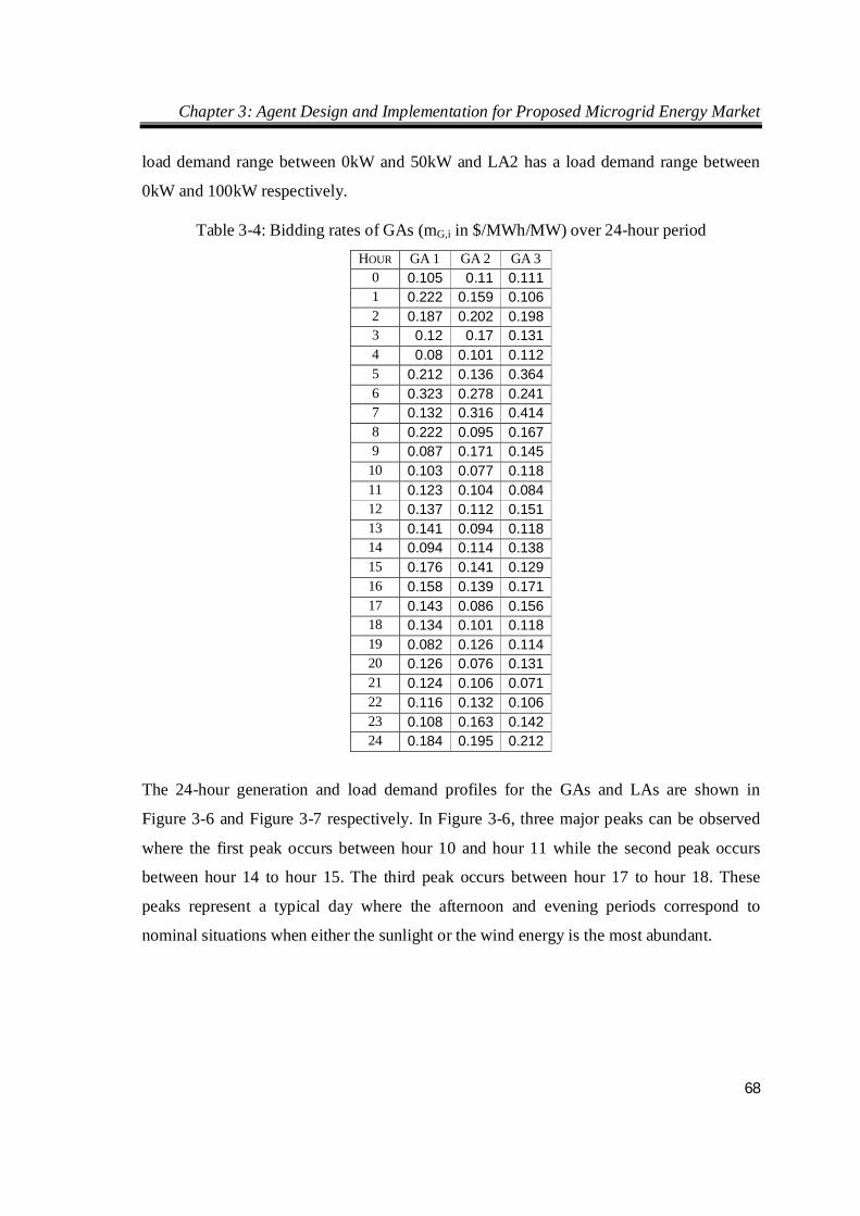
Chapter 3: Agent Design and Implementation for Proposed Microgrid Energy Market
68
load demand range between 0kW and 50kW and LA2 has a load demand range between
0kW and 100kW respectively.
Table 3-4: Bidding rates of GAs (mG,i in $/MWh/MW) over 24-hour period
HOUR GA 1 GA 2 GA 3 0 0.105 0.11 0.111 1 0.222 0.159 0.106 2 0.187 0.202 0.198 3 0.12 0.17 0.131 4 0.08 0.101 0.112 5 0.212 0.136 0.364 6 0.323 0.278 0.241 7 0.132 0.316 0.414 8 0.222 0.095 0.167 9 0.087 0.171 0.145
10 0.103 0.077 0.118 11 0.123 0.104 0.084 12 0.137 0.112 0.151 13 0.141 0.094 0.118 14 0.094 0.114 0.138 15 0.176 0.141 0.129 16 0.158 0.139 0.171 17 0.143 0.086 0.156 18 0.134 0.101 0.118 19 0.082 0.126 0.114 20 0.126 0.076 0.131 21 0.124 0.106 0.071 22 0.116 0.132 0.106 23 0.108 0.163 0.142 24 0.184 0.195 0.212
The 24-hour generation and load demand profiles for the GAs and LAs are shown in
Figure 3-6 and Figure 3-7 respectively. In Figure 3-6, three major peaks can be observed
where the first peak occurs between hour 10 and hour 11 while the second peak occurs
between hour 14 to hour 15. The third peak occurs between hour 17 to hour 18. These
peaks represent a typical day where the afternoon and evening periods correspond to
nominal situations when either the sunlight or the wind energy is the most abundant.
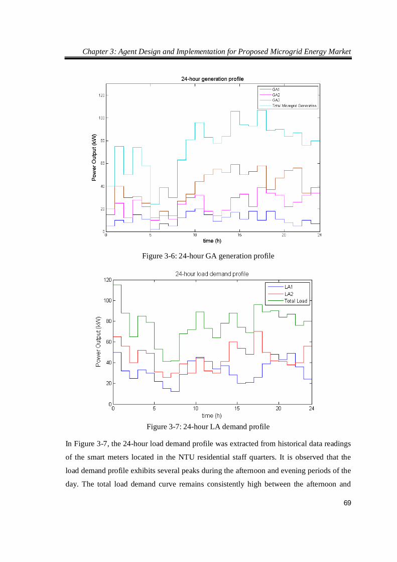
Chapter 3: Agent Design and Implementation for Proposed Microgrid Energy Market
69
Figure 3-6: 24-hour GA generation profile
Figure 3-7: 24-hour LA demand profile
In Figure 3-7, the 24-hour load demand profile was extracted from historical data readings
of the smart meters located in the NTU residential staff quarters. It is observed that the
load demand profile exhibits several peaks during the afternoon and evening periods of the
day. The total load demand curve remains consistently high between the afternoon and
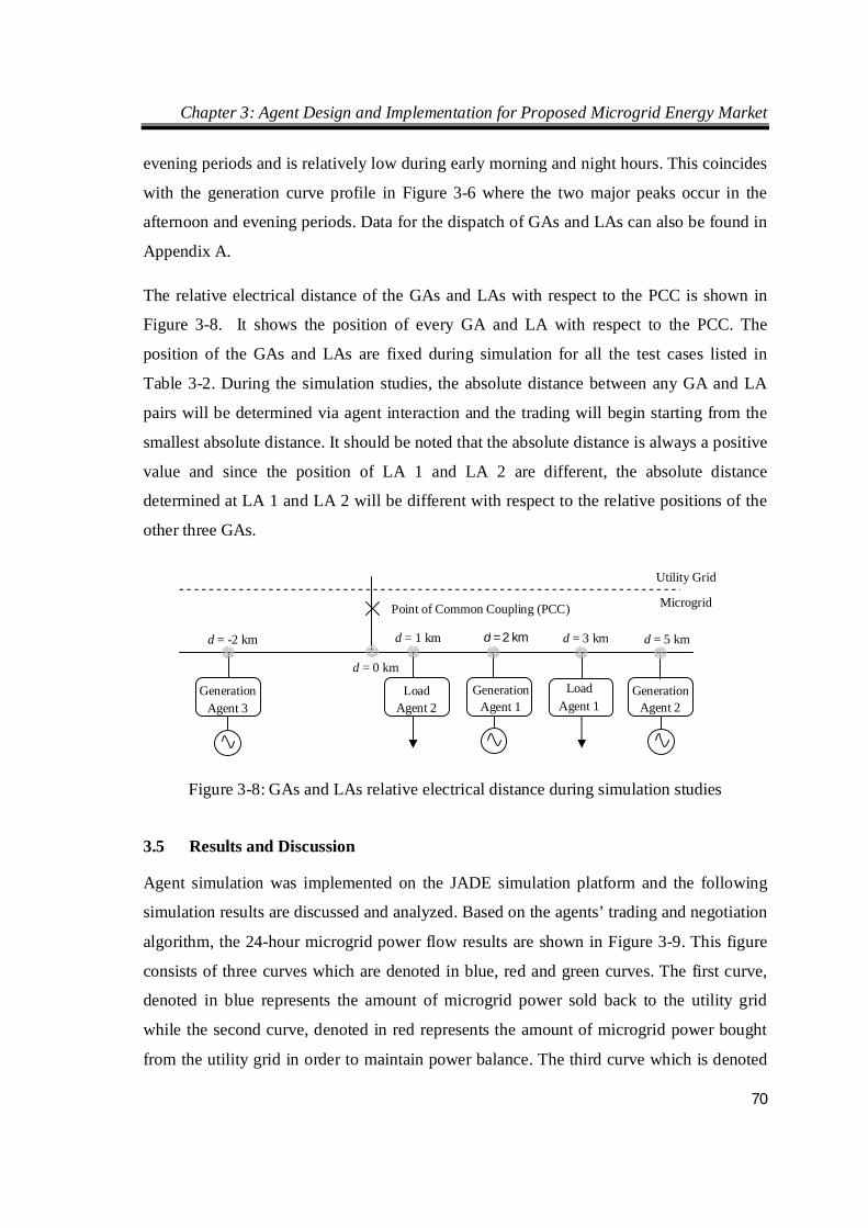
Chapter 3: Agent Design and Implementation for Proposed Microgrid Energy Market
70
evening periods and is relatively low during early morning and night hours. This coincides
with the generation curve profile in Figure 3-6 where the two major peaks occur in the
afternoon and evening periods. Data for the dispatch of GAs and LAs can also be found in
Appendix A.
The relative electrical distance of the GAs and LAs with respect to the PCC is shown in
Figure 3-8. It shows the position of every GA and LA with respect to the PCC. The
position of the GAs and LAs are fixed during simulation for all the test cases listed in
Table 3-2. During the simulation studies, the absolute distance between any GA and LA
pairs will be determined via agent interaction and the trading will begin starting from the
smallest absolute distance. It should be noted that the absolute distance is always a positive
value and since the position of LA 1 and LA 2 are different, the absolute distance
determined at LA 1 and LA 2 will be different with respect to the relative positions of the
other three GAs.
Figure 3-8: GAs and LAs relative electrical distance during simulation studies
3.5 Results and Discussion
Agent simulation was implemented on the JADE simulation platform and the following
simulation results are discussed and analyzed. Based on the agents’ trading and negotiation
algorithm, the 24-hour microgrid power flow results are shown in Figure 3-9. This figure
consists of three curves which are denoted in blue, red and green curves. The first curve,
denoted in blue represents the amount of microgrid power sold back to the utility grid
while the second curve, denoted in red represents the amount of microgrid power bought
from the utility grid in order to maintain power balance. The third curve which is denoted
Generation Agent 3
Load Agent 1
Load Agent 2
Generation Agent 1
Generation Agent 2
Point of Common Coupling (PCC) Microgrid
Utility Grid
d = 3 km d = 2 km d = 5 km d = -2 km d = 1 km
d = 0 km
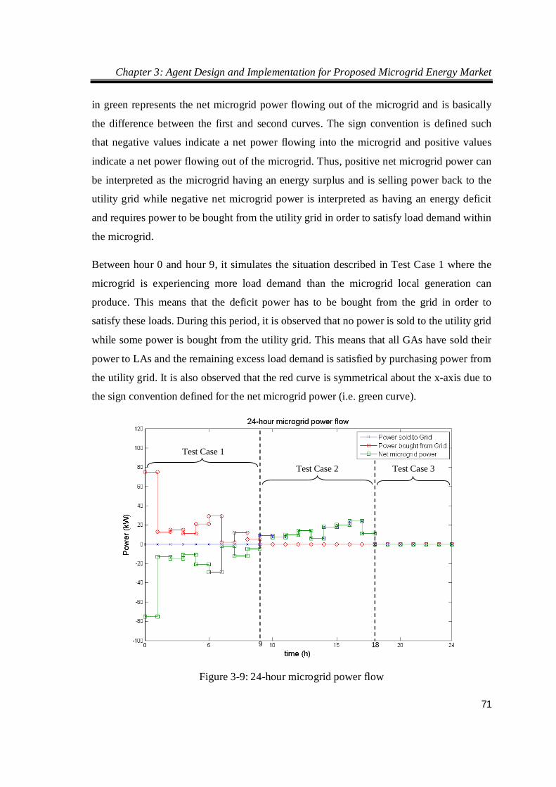
Chapter 3: Agent Design and Implementation for Proposed Microgrid Energy Market
71
in green represents the net microgrid power flowing out of the microgrid and is basically
the difference between the first and second curves. The sign convention is defined such
that negative values indicate a net power flowing into the microgrid and positive values
indicate a net power flowing out of the microgrid. Thus, positive net microgrid power can
be interpreted as the microgrid having an energy surplus and is selling power back to the
utility grid while negative net microgrid power is interpreted as having an energy deficit
and requires power to be bought from the utility grid in order to satisfy load demand within
the microgrid.
Between hour 0 and hour 9, it simulates the situation described in Test Case 1 where the
microgrid is experiencing more load demand than the microgrid local generation can
produce. This means that the deficit power has to be bought from the grid in order to
satisfy these loads. During this period, it is observed that no power is sold to the utility grid
while some power is bought from the utility grid. This means that all GAs have sold their
power to LAs and the remaining excess load demand is satisfied by purchasing power from
the utility grid. It is also observed that the red curve is symmetrical about the x-axis due to
the sign convention defined for the net microgrid power (i.e. green curve).
Figure 3-9: 24-hour microgrid power flow
Test Case 1
Test Case 2 Test Case 3
9 18
Chapter 3: Agent Design and Implementation for Proposed Microgrid Energy Market
72
Between hour 9 and hour 18, the situation described in Test Case 2 is simulated where the
microgrid is experiencing a net surplus of power. It is observed that no power is bought
from the utility grid while some power is sold to the utility grid during this period. This
means that all LA load demand are satisfied by the GAs and the remaining excess GA
generation is sold back to the utility grid. During this period, the green curve overlaps with
the blue curve because both indicate that power is flowing out of the microgrid.
Between hour 18 to hour 24, the situation described in Test Case 3 is simulated where the
microgrid is experiencing zero net microgrid power flow. During this period, there is no
power sold and bought from the utility grid. This indicates that the power generated from
the GAs equals the load demand of the LAs within the microgrid. Under such condition,
trading and negotiation occurs only between the GAs and LAs and no transactions are
made with the utility grid.
Next, Figure 3-10 illustrates the MCP under various agent objectives. The grid selling
price and grid buyback price in this simulation study is set at $4/kWh and $3.4/kWh
respectively. In this figure, three curves which are denoted by green, red and blue bars are
presented. The first curve, identified by a blue bar, is the computed MCP curve which
denotes the actual MCP calculated by PA. The second curve, identified by a red bar, is the
maximization of load benefits curve. The third curve, identified by a green bar, is the
maximization of GA profits curve. Numerical data of the MCP under various agent
objectives can also be found in Appendix A.
In Figure 3-10, it is observed that there are periods when the computed MCP is above the
grid selling price and several instances when it is below the grid buyback price. However
for maximization of load benefits price curve, the clearing price is capped at the grid
selling price but it is allowed to fall below the grid buyback price. The reason for the
clearing price to cap at the grid selling price is to ensure that the price offered by GAs is at
least the same or lower than the utility grid. For GAs adopting this strategy, they will
follow this price curve to sell their power.
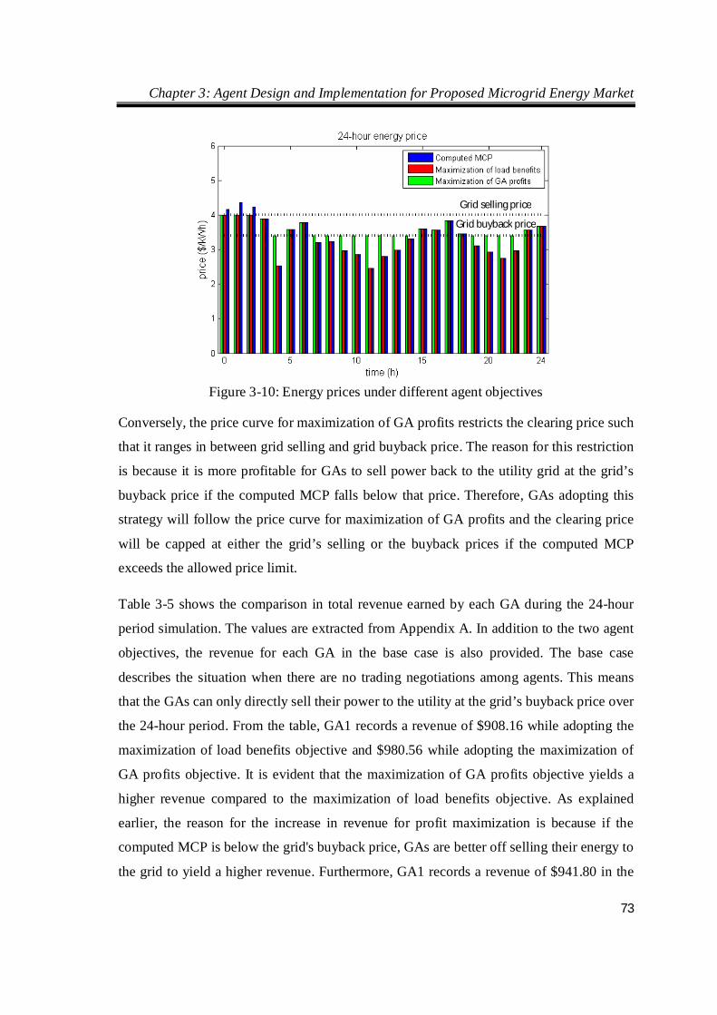
Chapter 3: Agent Design and Implementation for Proposed Microgrid Energy Market
73
Figure 3-10: Energy prices under different agent objectives
Conversely, the price curve for maximization of GA profits restricts the clearing price such
that it ranges in between grid selling and grid buyback price. The reason for this restriction
is because it is more profitable for GAs to sell power back to the utility grid at the grid’s
buyback price if the computed MCP falls below that price. Therefore, GAs adopting this
strategy will follow the price curve for maximization of GA profits and the clearing price
will be capped at either the grid’s selling or the buyback prices if the computed MCP
exceeds the allowed price limit.
Table 3-5 shows the comparison in total revenue earned by each GA during the 24-hour
period simulation. The values are extracted from Appendix A. In addition to the two agent
objectives, the revenue for each GA in the base case is also provided. The base case
describes the situation when there are no trading negotiations among agents. This means
that the GAs can only directly sell their power to the utility at the grid’s buyback price over
the 24-hour period. From the table, GA1 records a revenue of $908.16 while adopting the
maximization of load benefits objective and $980.56 while adopting the maximization of
GA profits objective. It is evident that the maximization of GA profits objective yields a
higher revenue compared to the maximization of load benefits objective. As explained
earlier, the reason for the increase in revenue for profit maximization is because if the
computed MCP is below the grid's buyback price, GAs are better off selling their energy to
the grid to yield a higher revenue. Furthermore, GA1 records a revenue of $941.80 in the
Grid selling price
Grid buyback price
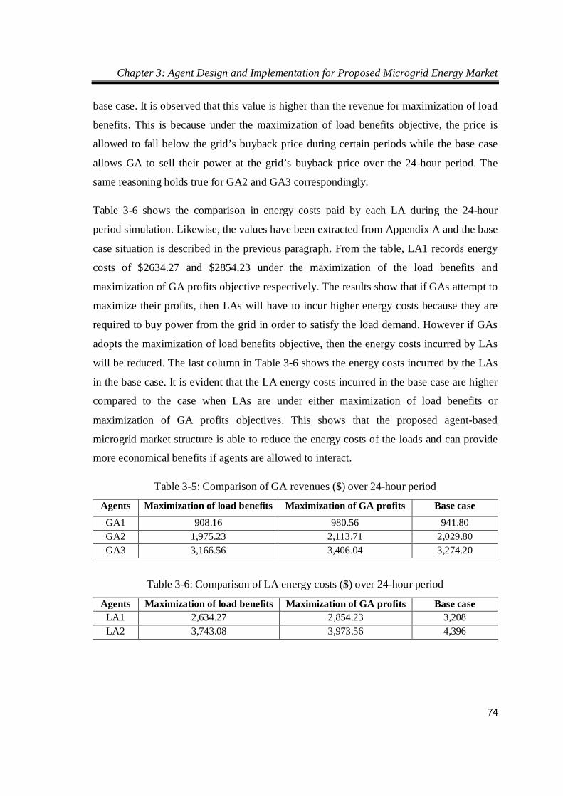
Chapter 3: Agent Design and Implementation for Proposed Microgrid Energy Market
74
base case. It is observed that this value is higher than the revenue for maximization of load
benefits. This is because under the maximization of load benefits objective, the price is
allowed to fall below the grid’s buyback price during certain periods while the base case
allows GA to sell their power at the grid’s buyback price over the 24-hour period. The
same reasoning holds true for GA2 and GA3 correspondingly.
Table 3-6 shows the comparison in energy costs paid by each LA during the 24-hour
period simulation. Likewise, the values have been extracted from Appendix A and the base
case situation is described in the previous paragraph. From the table, LA1 records energy
costs of $2634.27 and $2854.23 under the maximization of the load benefits and
maximization of GA profits objective respectively. The results show that if GAs attempt to
maximize their profits, then LAs will have to incur higher energy costs because they are
required to buy power from the grid in order to satisfy the load demand. However if GAs
adopts the maximization of load benefits objective, then the energy costs incurred by LAs
will be reduced. The last column in Table 3-6 shows the energy costs incurred by the LAs
in the base case. It is evident that the LA energy costs incurred in the base case are higher
compared to the case when LAs are under either maximization of load benefits or
maximization of GA profits objectives. This shows that the proposed agent-based
microgrid market structure is able to reduce the energy costs of the loads and can provide
more economical benefits if agents are allowed to interact.
Table 3-5: Comparison of GA revenues ($) over 24-hour period
Agents Maximization of load benefits Maximization of GA profits Base case GA1 908.16 980.56 941.80 GA2 1,975.23 2,113.71 2,029.80 GA3 3,166.56 3,406.04 3,274.20
Table 3-6: Comparison of LA energy costs ($) over 24-hour period
Agents Maximization of load benefits Maximization of GA profits Base case LA1 2,634.27 2,854.23 3,208 LA2 3,743.08 3,973.56 4,396
Chapter 3: Agent Design and Implementation for Proposed Microgrid Energy Market
75
3.6 Summary
This chapter presents the application of MAS when running the proposed local microgrid
market clearing algorithm using JADE. It basically provides a platform for agents to
communicate and to perform the required market operations and monitoring tasks.
Simulation was done in compliance with the IEEE FIPA standard through the use of JADE
which uses the AMS and DF agents to manage the agent platform. It is found that the
maximization of load benefits objective minimizes the profit of GAs while the profit
maximization of GAs objective minimizes the benefits of LAs. This shows that the two
agent objectives are biased to either the LAs or GAs. Therefore, a new agent objective is
required to promote unbiased transactions between the agents. This is implemented and
analyzed in the next chapter.
Under the proposed distributed agent-based control scheme, design and development of
user-defined agents and their respective GUIs were created. Agent simulation was
implemented on JADE to test the functionalities of the user-defined agents. During market
trading, agents are programmed to consider the MCP, agent's objective and RED between
each other as part of the criteria to perform power balancing and trading negotiations. The
simulation results have shown that MAS is able to manage a distributed local energy
trading market for DGs and loads to engage in negotiations while considering different
microgrid conditions.
The simulation study in this chapter considers the single-side bidding mechanism of DGs
and loads in the microgrid. In order to study the full market interaction between DGs and
loads, a double-side bidding mechanism is required which will be covered in the next
chapter. The simulation environment developed in this chapter primarily discusses the
market interaction between agents which also serves as a reference for detailed studies in
the next chapter where the t-domain dynamics of MW generation and bus voltage profiles
are considered using the proposed microgrid market clearing technique.
Chapter 4: Multi Agent System for Distributed Management of Microgrids
76
CHAPTER 4 MUTLI AGENT SYSTEM FOR
DISTRIBUTED MANAGEMENT OF
MICROGRIDS
4.1 Introduction
As mentioned in Chapter 1, MAS is proposed for generation and demand scheduling and
the LMP for various participants in the distributed microgrid energy market. Generator and
load agents retrieve power scheduling information based on their incremental cost and
price signals obtained from the proposed microgrid energy market. The power reference
and load control signals are then sent to the generator and load correspondingly. The price
signal refers to the Market Clearing Price (MCP) which is derived from the submitted bids
of the generator and load. Subsequently, the derived MCP establishes the price reference in
LMP among other variables where the participants will pay or be paid at that price. The
amount that each generator or load agent receives or pays respectively depends on some
objectives imposed on the agents.
4.2 Problem Formulation
4.2.1 MCP (Double Side Bidding) and Scheduling Problem
The idea of proposing a microgrid market structure is to encourage a competitive
electricity market since DERs are considered more economical to generate electricity
locally at least for a certain peak period compared to buying it directly from the main grid
[77, 135]. In addition, a real-time market clearing technique is used to determine the MCP.
The objective in determining MCP is to dispatch an aggregate of different types of DGs to
an aggregate of different consumers. In Chapter 3, single side bidding was considered for
the microgrid market bidding mechanism because it is assumed that consumers have no
expertise to contribute effectively in the price mechanism. Therefore, most electricity
markets consider consumers to be incapable of making rational market decisions and are
simply represented as fixed loads which need to be satisfied. Therefore, active consumer
participation in energy markets remains minimal. However, due to the advancement in
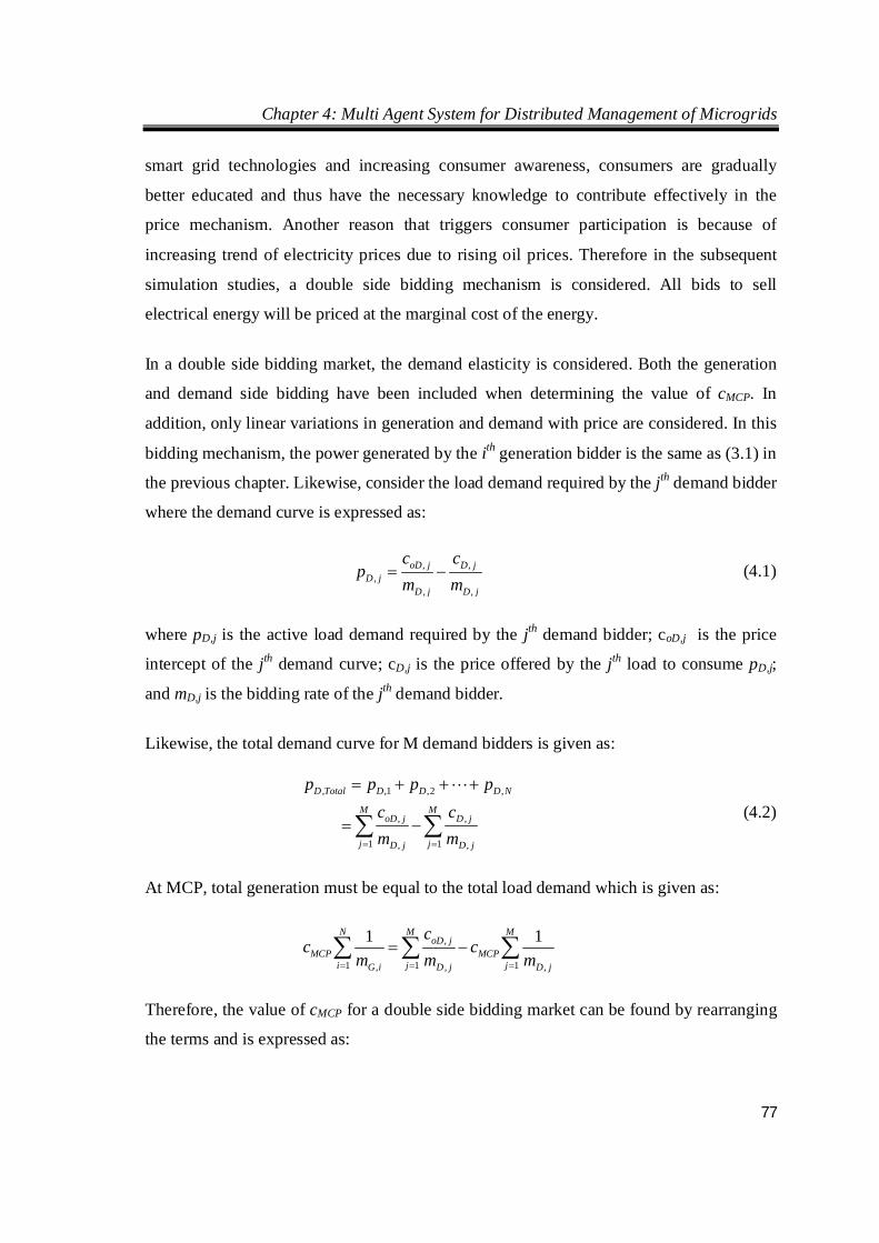
Chapter 4: Multi Agent System for Distributed Management of Microgrids
77
smart grid technologies and increasing consumer awareness, consumers are gradually
better educated and thus have the necessary knowledge to contribute effectively in the
price mechanism. Another reason that triggers consumer participation is because of
increasing trend of electricity prices due to rising oil prices. Therefore in the subsequent
simulation studies, a double side bidding mechanism is considered. All bids to sell
electrical energy will be priced at the marginal cost of the energy.
In a double side bidding market, the demand elasticity is considered. Both the generation
and demand side bidding have been included when determining the value of cMCP. In
addition, only linear variations in generation and demand with price are considered. In this
bidding mechanism, the power generated by the ith generation bidder is the same as (3.1) in
the previous chapter. Likewise, consider the load demand required by the jth demand bidder
where the demand curve is expressed as:
, ,,
, ,
oD j D jD j
D j D j
c cp
m m (4.1)
where pD,j is the active load demand required by the jth demand bidder; coD,j is the price
intercept of the jth demand curve; cD,j is the price offered by the jth load to consume pD,j;
and mD,j is the bidding rate of the jth demand bidder.
Likewise, the total demand curve for M demand bidders is given as:
, ,1 ,2 ,
, ,
1 1, ,
D Total D D D N
M MoD j D j
j jD j D j
p p p pc cm m
(4.2)
At MCP, total generation must be equal to the total load demand which is given as:
,
1 1 1, , ,
1 1N M MoD j
MCP MCPi j jG i D j D j
cc c
m m m
Therefore, the value of cMCP for a double side bidding market can be found by rearranging
the terms and is expressed as:
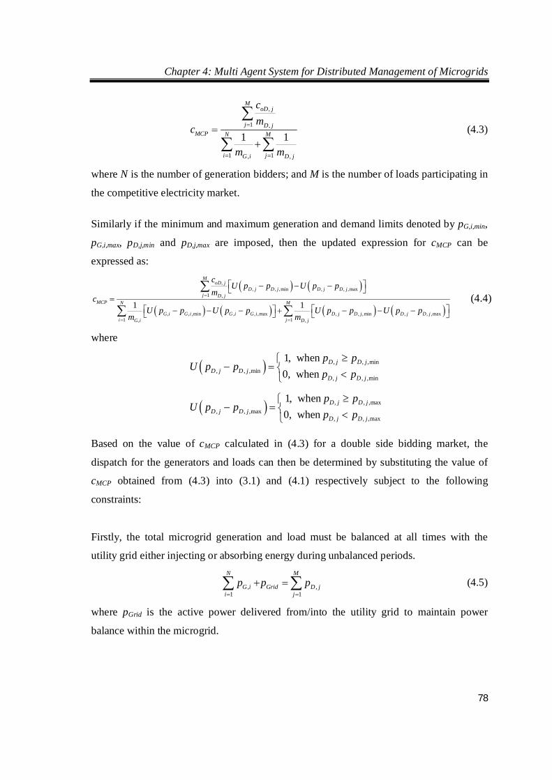
Chapter 4: Multi Agent System for Distributed Management of Microgrids
78
,
1 ,
1 1, ,
1 1
MoD j
j D jMCP N M
i jG i D j
cm
c
m m
(4.3)
where N is the number of generation bidders; and M is the number of loads participating in
the competitive electricity market.
Similarly if the minimum and maximum generation and demand limits denoted by pG,i,min,
pG,i,max, pD,j,min and pD,j,max are imposed, then the updated expression for cMCP can be
expressed as:
,, , ,min , , ,max
1 ,
, , ,min , , ,max , , ,min , , ,max1 1, ,
1 1
MoD j
D j D j D j D jj D j
MCP N M
G i G i G i G i D j D j D j D ji jG i D j
cU p p U p p
mc
U p p U p p U p p U p pm m
(4.4)
where
, , ,min, , ,min
, , ,min
1, when 0, when
D j D jD j D j
D j D j
p pU p p
p p
, , ,max, , ,max
, , ,max
1, when 0, when
D j D jD j D j
D j D j
p pU p p
p p
Based on the value of cMCP calculated in (4.3) for a double side bidding market, the
dispatch for the generators and loads can then be determined by substituting the value of
cMCP obtained from (4.3) into (3.1) and (4.1) respectively subject to the following
constraints:
Firstly, the total microgrid generation and load must be balanced at all times with the
utility grid either injecting or absorbing energy during unbalanced periods.
, ,1 1
N M
G i Grid D ji j
p p p
(4.5)
where pGrid is the active power delivered from/into the utility grid to maintain power
balance within the microgrid.
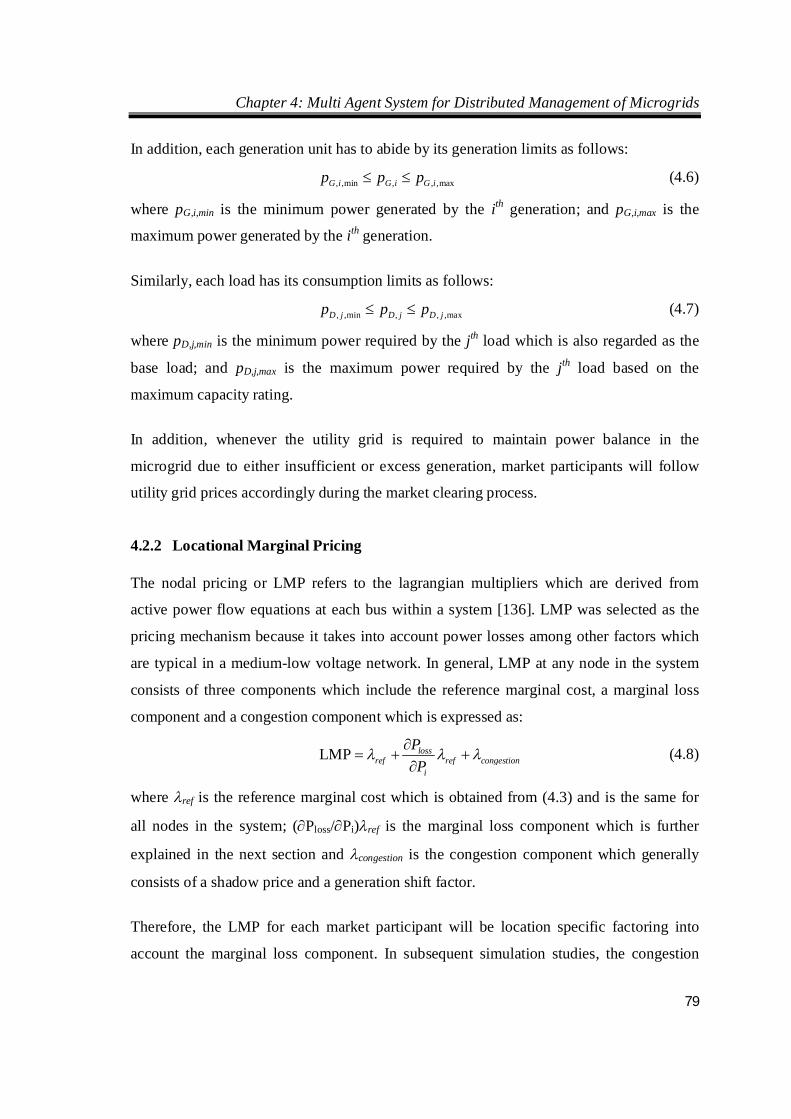
Chapter 4: Multi Agent System for Distributed Management of Microgrids
79
In addition, each generation unit has to abide by its generation limits as follows:
, ,min , , ,maxG i G i G ip p p (4.6)
where pG,i,min is the minimum power generated by the ith generation; and pG,i,max is the
maximum power generated by the ith generation.
Similarly, each load has its consumption limits as follows:
, ,min , , ,maxD j D j D jp p p (4.7)
where pD,j,min is the minimum power required by the jth load which is also regarded as the
base load; and pD,j,max is the maximum power required by the jth load based on the
maximum capacity rating.
In addition, whenever the utility grid is required to maintain power balance in the
microgrid due to either insufficient or excess generation, market participants will follow
utility grid prices accordingly during the market clearing process.
4.2.2 Locational Marginal Pricing
The nodal pricing or LMP refers to the lagrangian multipliers which are derived from
active power flow equations at each bus within a system [136]. LMP was selected as the
pricing mechanism because it takes into account power losses among other factors which
are typical in a medium-low voltage network. In general, LMP at any node in the system
consists of three components which include the reference marginal cost, a marginal loss
component and a congestion component which is expressed as:
LMP lossref ref congestion
i
PP
(4.8)
where ref is the reference marginal cost which is obtained from (4.3) and is the same for
all nodes in the system; (Ploss/Pi)ref is the marginal loss component which is further
explained in the next section and congestion is the congestion component which generally
consists of a shadow price and a generation shift factor.
Therefore, the LMP for each market participant will be location specific factoring into
account the marginal loss component. In subsequent simulation studies, the congestion
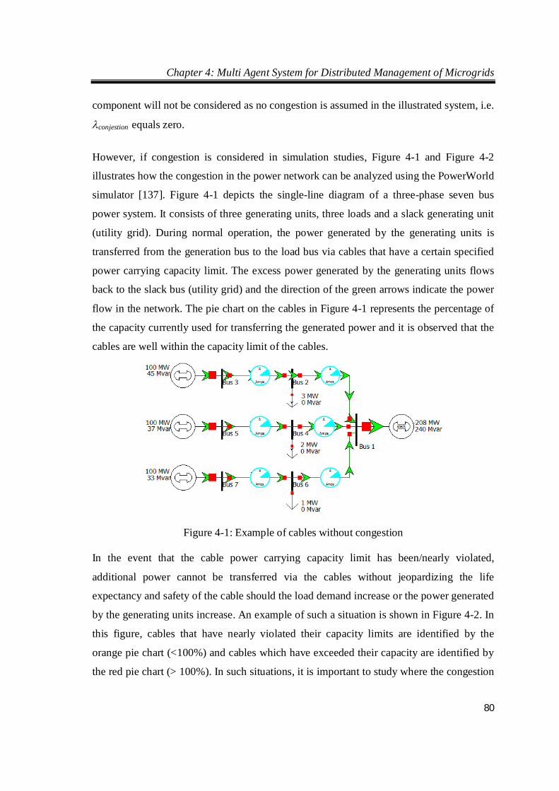
Chapter 4: Multi Agent System for Distributed Management of Microgrids
80
component will not be considered as no congestion is assumed in the illustrated system, i.e.
conjestion equals zero.
However, if congestion is considered in simulation studies, Figure 4-1 and Figure 4-2
illustrates how the congestion in the power network can be analyzed using the PowerWorld
simulator [137]. Figure 4-1 depicts the single-line diagram of a three-phase seven bus
power system. It consists of three generating units, three loads and a slack generating unit
(utility grid). During normal operation, the power generated by the generating units is
transferred from the generation bus to the load bus via cables that have a certain specified
power carrying capacity limit. The excess power generated by the generating units flows
back to the slack bus (utility grid) and the direction of the green arrows indicate the power
flow in the network. The pie chart on the cables in Figure 4-1 represents the percentage of
the capacity currently used for transferring the generated power and it is observed that the
cables are well within the capacity limit of the cables.
Figure 4-1: Example of cables without congestion
In the event that the cable power carrying capacity limit has been/nearly violated,
additional power cannot be transferred via the cables without jeopardizing the life
expectancy and safety of the cable should the load demand increase or the power generated
by the generating units increase. An example of such a situation is shown in Figure 4-2. In
this figure, cables that have nearly violated their capacity limits are identified by the
orange pie chart (<100%) and cables which have exceeded their capacity are identified by
the red pie chart (> 100%). In such situations, it is important to study where the congestion
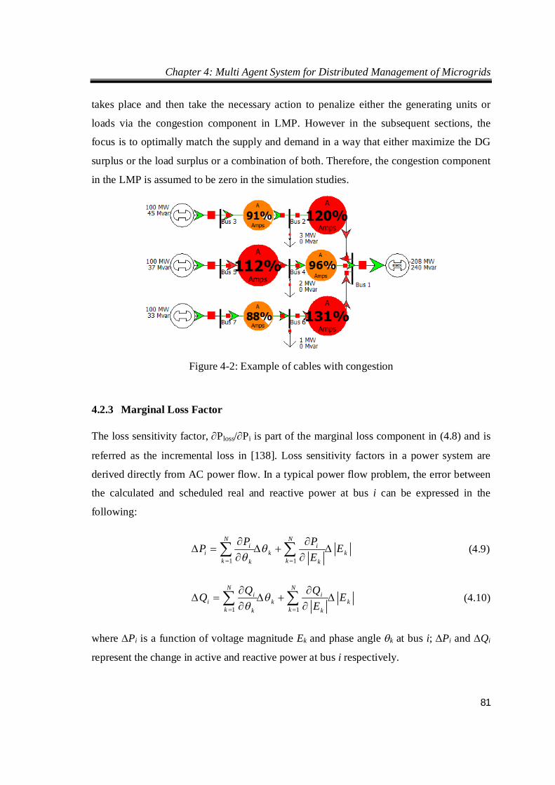
Chapter 4: Multi Agent System for Distributed Management of Microgrids
81
takes place and then take the necessary action to penalize either the generating units or
loads via the congestion component in LMP. However in the subsequent sections, the
focus is to optimally match the supply and demand in a way that either maximize the DG
surplus or the load surplus or a combination of both. Therefore, the congestion component
in the LMP is assumed to be zero in the simulation studies.
Figure 4-2: Example of cables with congestion
4.2.3 Marginal Loss Factor
The loss sensitivity factor, Ploss/Pi is part of the marginal loss component in (4.8) and is
referred as the incremental loss in [138]. Loss sensitivity factors in a power system are
derived directly from AC power flow. In a typical power flow problem, the error between
the calculated and scheduled real and reactive power at bus i can be expressed in the
following:
1 1
N Ni i
i k kk kk k
P PP EE
(4.9)
1 1
N Ni i
i k kk kk k
Q QQ EE
(4.10)
where Pi is a function of voltage magnitude Ek and phase angle k at bus i; Pi and Qi
represent the change in active and reactive power at bus i respectively.
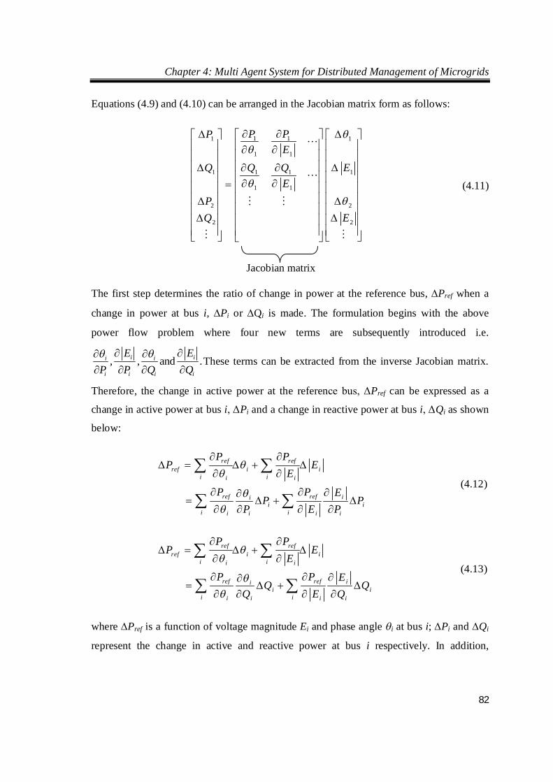
Chapter 4: Multi Agent System for Distributed Management of Microgrids
82
Equations (4.9) and (4.10) can be arranged in the Jacobian matrix form as follows:
1 11 1
1 1
1 1 1 1
1 1
2 2
2 2
P PPE
Q Q Q EE
PQ E
(4.11)
The first step determines the ratio of change in power at the reference bus, Pref when a
change in power at bus i, Pi or Qi is made. The formulation begins with the above
power flow problem where four new terms are subsequently introduced i.e.
, , and .i ii i
i i i i
E EP P Q Q
These terms can be extracted from the inverse Jacobian matrix.
Therefore, the change in active power at the reference bus, ΔPref can be expressed as a
change in active power at bus i, ΔPi and a change in reactive power at bus i, ΔQi as shown
below:
ref refref i i
i ii i
ref ref iii i
i ii i i i
P PP E
E
P P EP P
P E P
(4.12)
ref refref i i
i ii i
ref ref iii i
i ii i i i
P PP E
EP P E
Q QQ E Q
(4.13)
where Pref is a function of voltage magnitude Ei and phase angle i at bus i; Pi and Qi
represent the change in active and reactive power at bus i respectively. In addition,
Jacobian matrix
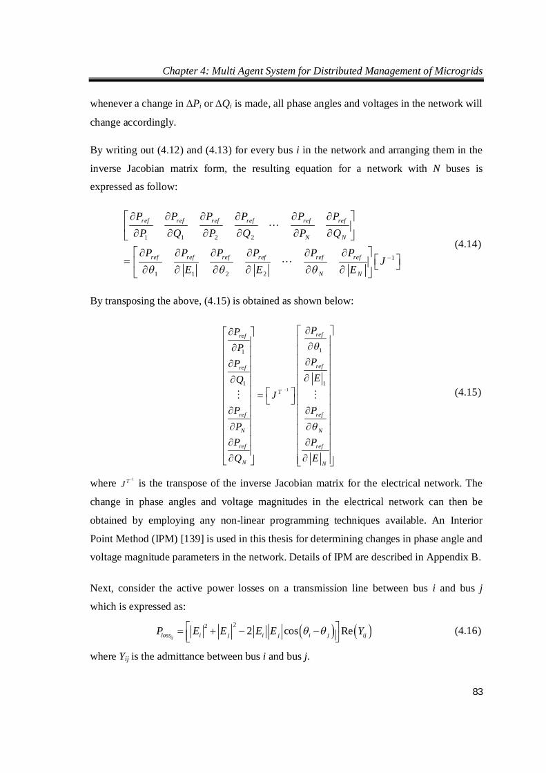
Chapter 4: Multi Agent System for Distributed Management of Microgrids
83
whenever a change in Pi or Qi is made, all phase angles and voltages in the network will
change accordingly.
By writing out (4.12) and (4.13) for every bus i in the network and arranging them in the
inverse Jacobian matrix form, the resulting equation for a network with N buses is
expressed as follow:
1 1 2 2
1
1 1 2 2
ref ref ref ref ref ref
N N
ref ref ref ref ref ref
N N
P P P P P PP Q P Q P Q
P P P P P PJ
E E E
(4.14)
By transposing the above, (4.15) is obtained as shown below:
1
11
1 1
refref
refref
T
ref ref
N N
ref ref
N N
PPP
PPEQ
JP PPP PQ E
(4.15)
where 1TJ is the transpose of the inverse Jacobian matrix for the electrical network. The
change in phase angles and voltage magnitudes in the electrical network can then be
obtained by employing any non-linear programming techniques available. An Interior
Point Method (IPM) [139] is used in this thesis for determining changes in phase angle and
voltage magnitude parameters in the network. Details of IPM are described in Appendix B.
Next, consider the active power losses on a transmission line between bus i and bus j
which is expressed as:
22 2 cos Reijloss i j i j i j ijP E E E E Y
(4.16)
where Yij is the admittance between bus i and bus j.
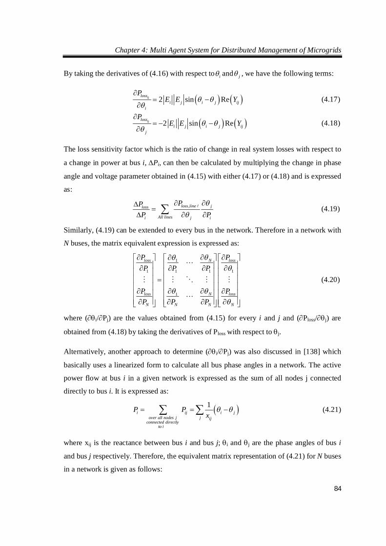
Chapter 4: Multi Agent System for Distributed Management of Microgrids
84
By taking the derivatives of (4.16) with respect to i and j , we have the following terms:
2 sin Reijlossi j i j ij
i
PE E Y
(4.17)
2 sin Reijlossi j i j ij
j
PE E Y
(4.18)
The loss sensitivity factor which is the ratio of change in real system losses with respect to
a change in power at bus i, Pi, can then be calculated by multiplying the change in phase
angle and voltage parameter obtained in (4.15) with either (4.17) or (4.18) and is expressed
as:
,loss line jloss
All linesi j i
PPP P
(4.19)
Similarly, (4.19) can be extended to every bus in the network. Therefore in a network with
N buses, the matrix equivalent expression is expressed as:
1
1 1 1 1
1
loss N loss
loss N loss
N N N N
P PP P P
P PP P P
(4.20)
where (i/Pj) are the values obtained from (4.15) for every i and j and (Ploss/j) are
obtained from (4.18) by taking the derivatives of Ploss with respect to j.
Alternatively, another approach to determine (i/Pj) was also discussed in [138] which
basically uses a linearized form to calculate all bus phase angles in a network. The active
power flow at bus i in a given network is expressed as the sum of all nodes j connected
directly to bus i. It is expressed as:
1i ij i j
over all nodes j j ijconnected directly
to i
P Px
(4.21)
where xij is the reactance between bus i and bus j; i and j are the phase angles of bus i
and bus j respectively. Therefore, the equivalent matrix representation of (4.21) for N buses
in a network is given as follows:
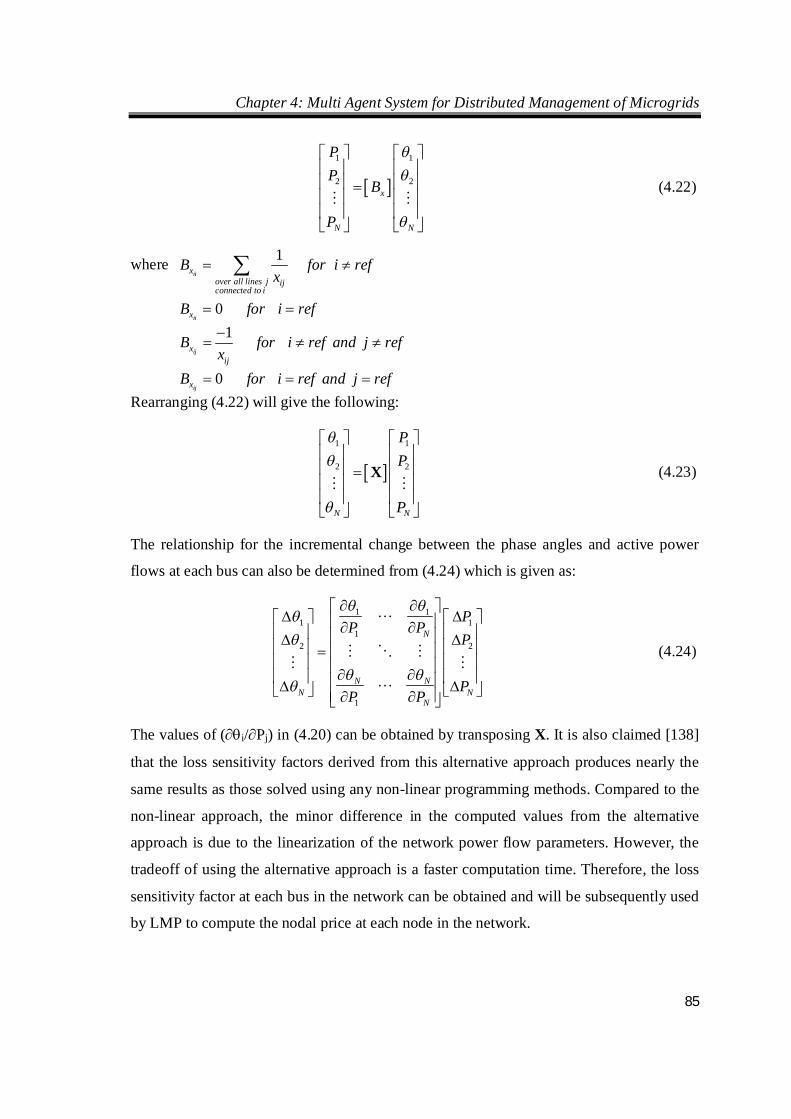
Chapter 4: Multi Agent System for Distributed Management of Microgrids
85
1 1
2 2x
N N
PP
B
P
(4.22)
where 1iix
over all lines j ijconnected to i
B for i refx
0iixB for i ref
1ijx
ij
B for i ref and j refx
0ijxB for i ref and j ref
Rearranging (4.22) will give the following:
1 1
2 2
N N
PP
P
X
(4.23)
The relationship for the incremental change between the phase angles and active power
flows at each bus can also be determined from (4.24) which is given as:
1 11 1
12 2
1
N
N NN N
N
PP P
P
PP P
(4.24)
The values of (i/Pj) in (4.20) can be obtained by transposing X. It is also claimed [138]
that the loss sensitivity factors derived from this alternative approach produces nearly the
same results as those solved using any non-linear programming methods. Compared to the
non-linear approach, the minor difference in the computed values from the alternative
approach is due to the linearization of the network power flow parameters. However, the
tradeoff of using the alternative approach is a faster computation time. Therefore, the loss
sensitivity factor at each bus in the network can be obtained and will be subsequently used
by LMP to compute the nodal price at each node in the network.
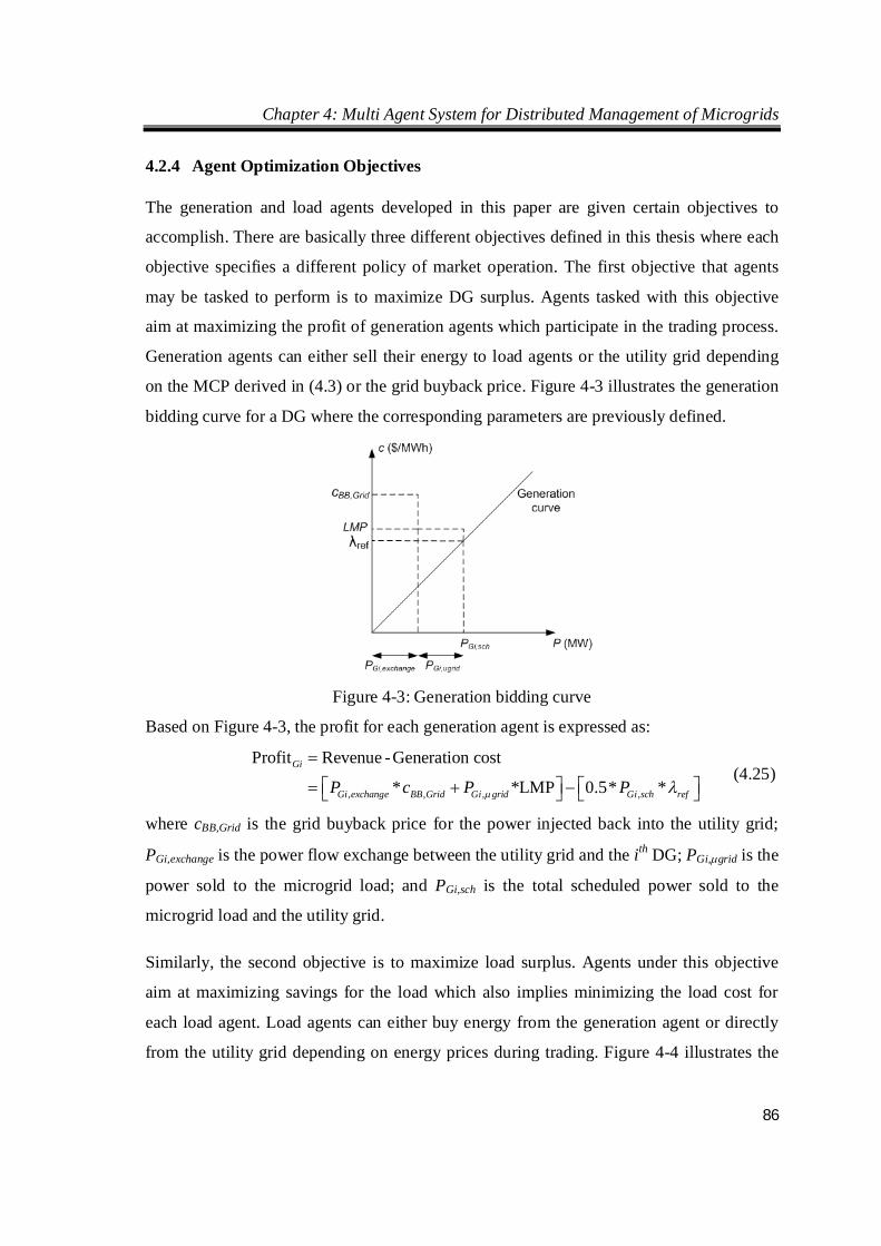
Chapter 4: Multi Agent System for Distributed Management of Microgrids
86
4.2.4 Agent Optimization Objectives
The generation and load agents developed in this paper are given certain objectives to
accomplish. There are basically three different objectives defined in this thesis where each
objective specifies a different policy of market operation. The first objective that agents
may be tasked to perform is to maximize DG surplus. Agents tasked with this objective
aim at maximizing the profit of generation agents which participate in the trading process.
Generation agents can either sell their energy to load agents or the utility grid depending
on the MCP derived in (4.3) or the grid buyback price. Figure 4-3 illustrates the generation
bidding curve for a DG where the corresponding parameters are previously defined.
Figure 4-3: Generation bidding curve
Based on Figure 4-3, the profit for each generation agent is expressed as:
, , , ,
Profit Revenue -Generation cost
* *LMP 0.5* *Gi
Gi exchange BB Grid Gi grid Gi sch refP c P P
(4.25)
where cBB,Grid is the grid buyback price for the power injected back into the utility grid;
PGi,exchange is the power flow exchange between the utility grid and the ith DG; PGi,grid is the
power sold to the microgrid load; and PGi,sch is the total scheduled power sold to the
microgrid load and the utility grid.
Similarly, the second objective is to maximize load surplus. Agents under this objective
aim at maximizing savings for the load which also implies minimizing the load cost for
each load agent. Load agents can either buy energy from the generation agent or directly
from the utility grid depending on energy prices during trading. Figure 4-4 illustrates the
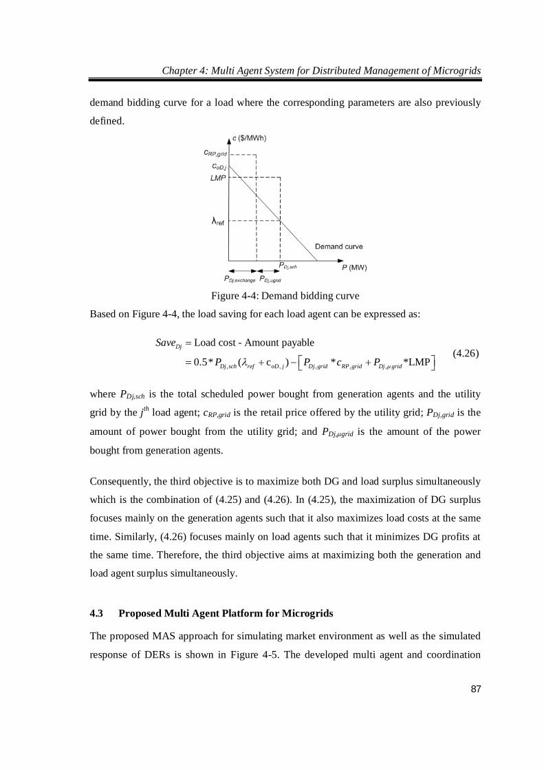
Chapter 4: Multi Agent System for Distributed Management of Microgrids
87
demand bidding curve for a load where the corresponding parameters are also previously
defined.
Figure 4-4: Demand bidding curve
Based on Figure 4-4, the load saving for each load agent can be expressed as:
, , , , ,
Load cost - Amount payable
0.5* ( c ) * *LMPDj
Dj sch ref oD j Dj grid RP grid Dj grid
Save
P P c P
(4.26)
where PDj,sch is the total scheduled power bought from generation agents and the utility
grid by the jth load agent; cRP,grid is the retail price offered by the utility grid; PDj,grid is the
amount of power bought from the utility grid; and PDj,grid is the amount of the power
bought from generation agents.
Consequently, the third objective is to maximize both DG and load surplus simultaneously
which is the combination of (4.25) and (4.26). In (4.25), the maximization of DG surplus
focuses mainly on the generation agents such that it also maximizes load costs at the same
time. Similarly, (4.26) focuses mainly on load agents such that it minimizes DG profits at
the same time. Therefore, the third objective aims at maximizing both the generation and
load agent surplus simultaneously.
4.3 Proposed Multi Agent Platform for Microgrids
The proposed MAS approach for simulating market environment as well as the simulated
response of DERs is shown in Figure 4-5. The developed multi agent and coordination
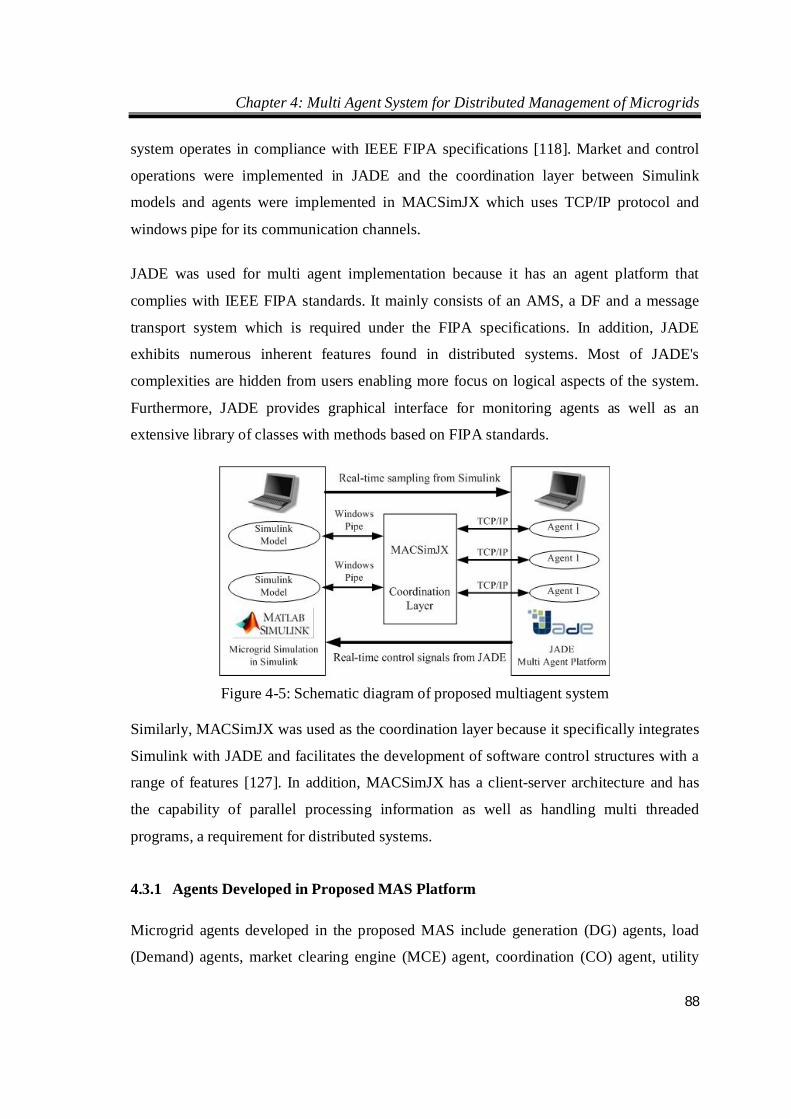
Chapter 4: Multi Agent System for Distributed Management of Microgrids
88
system operates in compliance with IEEE FIPA specifications [118]. Market and control
operations were implemented in JADE and the coordination layer between Simulink
models and agents were implemented in MACSimJX which uses TCP/IP protocol and
windows pipe for its communication channels.
JADE was used for multi agent implementation because it has an agent platform that
complies with IEEE FIPA standards. It mainly consists of an AMS, a DF and a message
transport system which is required under the FIPA specifications. In addition, JADE
exhibits numerous inherent features found in distributed systems. Most of JADE's
complexities are hidden from users enabling more focus on logical aspects of the system.
Furthermore, JADE provides graphical interface for monitoring agents as well as an
extensive library of classes with methods based on FIPA standards.
Figure 4-5: Schematic diagram of proposed multiagent system
Similarly, MACSimJX was used as the coordination layer because it specifically integrates
Simulink with JADE and facilitates the development of software control structures with a
range of features [127]. In addition, MACSimJX has a client-server architecture and has
the capability of parallel processing information as well as handling multi threaded
programs, a requirement for distributed systems.
4.3.1 Agents Developed in Proposed MAS Platform
Microgrid agents developed in the proposed MAS include generation (DG) agents, load
(Demand) agents, market clearing engine (MCE) agent, coordination (CO) agent, utility
Chapter 4: Multi Agent System for Distributed Management of Microgrids
89
grid (UG) agent, and other ancillary agents. A brief description of the functionalities for
the main agents are given below.
DG Agent: This agent models combined heat and power (CHP) units,
dispatchable units which may include MTs, fuel cells and energy storage systems
and non-dispatchable units which may include PVs and WTs as an aggregated
equivalent DG unit under the same owner to participate in microgrid market
operations through negotiations with Demand Agents. It also regulates and
controls output power and status of DG units. Information contained in this agent
includes an agent identifier, minimum and maximum generation limits and
dynamic data such as bidding rate, generation settings, revenue and DG surplus.
This agent have the basic functionalities similar to the Generation Agent (GA)
designed in Chapter 3 with the exception that the algorithm used during
scheduling and trading differs because LMP and load participation in the market
were considered in this Chapter.
Demand Agent: This agent models an aggregated equivalent load unit under the
same consumer to participate in market operations through negotiations with DG
Agents. It is also capable of regulating and controlling the power demand and
status of the respective load units based on energy prices. Information residing in
this agent includes an agent identifier, minimum and maximum demand limits
and dynamic data such as bidding rate, power demand settings, load costs and
savings. This agent retains the basic functionalities similar to the Load Agent
(LA) designed in Chapter 3 with the exception that the algorithm used for
scheduling and trading differs because the market participation of the loads are
considered in this Chapter.
MCE Agent: This agent becomes active if the MCP computation of the microgrid
is required for a specified period. It takes in bids from DG and Demand Agents
and liaises with CO Agent during market operations. Furthermore, it contains
aggregated information on microgrid generation and demand levels. This agent
have similar functions compared to the Price Agent (PA) designed in Chapter 3
with the exception that it will consider the bidding rate of the loads when
Chapter 4: Multi Agent System for Distributed Management of Microgrids
90
computing the MCP.
CO Agent: This agent is responsible for coordinating the entire microgrid market
operation as well as monitoring the network for any technical violations. It
coordinates with MACSimJX Agent to signal the beginning and end of market
operations for that period.
UG Agent: The utility grid agent basically behaves similar to an Independent
System Operator (ISO) and is responsible for power balance in the microgrid. It
also broadcasts retail price signals to DG and Demand Agents at regular intervals
to facilitate decision making in the corresponding agents.
MACSimJX Agent: This agent basically performs coordination between Simulink
and JADE as well as manages an Agent Task Force (ATF) which consists of
several ancillary agents to transmit simulink data to the CO, DG and Demand
Agents. These ancillary agents are the counterparts of the CO, DG and Demand
Agents that are represented in the ATF to transmit information to/from Simulink.
In addition, an Agent Environment (AE) residing within this agent also acts as an
interface for coordinating control signals between Simulink and JADE.
4.3.2 Agents Interaction and Coordination
A hierarchical control architecture [50, 51] is used for the simulation of microgrid
operation. The entire microgrid market operation and simulation are achieved by
distributing responsibilities to the various agents. Agents accomplish assigned tasks by
proactively interacting among themselves as shown in Figure 4-6. Generally, a typical
electricity market operation consists of a pre-gate and gate closure period. The gate closure
period occurs, say about an hour before the actual energy delivery time while the pre-gate
period occurs a few hours before the gate closure period. The pre-gate period is the time
when DGs and loads enter into negotiations to sell or buy a given quantity of electricity at
an agreed price. The gate closure period is the time when DGs and loads stop negotiating
and power balancing is executed to ensure that DGs and loads whose generation or load
demand are still not satisfied after negotiations have been balanced. Similarly, the
proposed market operation in this simulation study also adopts the pre-gate and gate
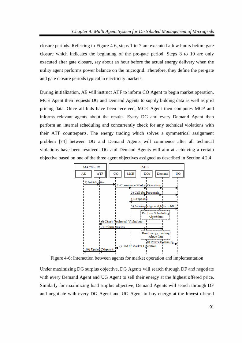
Chapter 4: Multi Agent System for Distributed Management of Microgrids
91
closure periods. Referring to Figure 4-6, steps 1 to 7 are executed a few hours before gate
closure which indicates the beginning of the pre-gate period. Steps 8 to 10 are only
executed after gate closure, say about an hour before the actual energy delivery when the
utility agent performs power balance on the microgrid. Therefore, they define the pre-gate
and gate closure periods typical in electricity markets.
During initialization, AE will instruct ATF to inform CO Agent to begin market operation.
MCE Agent then requests DG and Demand Agents to supply bidding data as well as grid
pricing data. Once all bids have been received, MCE Agent then computes MCP and
informs relevant agents about the results. Every DG and every Demand Agent then
perform an internal scheduling and concurrently check for any technical violations with
their ATF counterparts. The energy trading which solves a symmetrical assignment
problem [74] between DG and Demand Agents will commence after all technical
violations have been resolved. DG and Demand Agents will aim at achieving a certain
objective based on one of the three agent objectives assigned as described in Section 4.2.4.
Figure 4-6: Interaction between agents for market operation and implementation
Under maximizing DG surplus objective, DG Agents will search through DF and negotiate
with every Demand Agent and UG Agent to sell their energy at the highest offered price.
Similarly for maximizing load surplus objective, Demand Agents will search through DF
and negotiate with every DG Agent and UG Agent to buy energy at the lowest offered
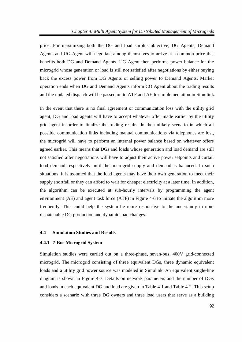
Chapter 4: Multi Agent System for Distributed Management of Microgrids
92
price. For maximizing both the DG and load surplus objective, DG Agents, Demand
Agents and UG Agent will negotiate among themselves to arrive at a common price that
benefits both DG and Demand Agents. UG Agent then performs power balance for the
microgrid whose generation or load is still not satisfied after negotiations by either buying
back the excess power from DG Agents or selling power to Demand Agents. Market
operation ends when DG and Demand Agents inform CO Agent about the trading results
and the updated dispatch will be passed on to ATF and AE for implementation in Simulink.
In the event that there is no final agreement or communication loss with the utility grid
agent, DG and load agents will have to accept whatever offer made earlier by the utility
grid agent in order to finalize the trading results. In the unlikely scenario in which all
possible communication links including manual communications via telephones are lost,
the microgrid will have to perform an internal power balance based on whatever offers
agreed earlier. This means that DGs and loads whose generation and load demand are still
not satisfied after negotiations will have to adjust their active power setpoints and curtail
load demand respectively until the microgrid supply and demand is balanced. In such
situations, it is assumed that the load agents may have their own generation to meet their
supply shortfall or they can afford to wait for cheaper electricity at a later time. In addition,
the algorithm can be executed at sub-hourly intervals by programming the agent
environment (AE) and agent task force (ATF) in Figure 4-6 to initiate the algorithm more
frequently. This could help the system be more responsive to the uncertainty in non-
dispatchable DG production and dynamic load changes.
4.4 Simulation Studies and Results
4.4.1 7-Bus Microgrid System
Simulation studies were carried out on a three-phase, seven-bus, 400V grid-connected
microgrid. The microgrid consisting of three equivalent DGs, three dynamic equivalent
loads and a utility grid power source was modeled in Simulink. An equivalent single-line
diagram is shown in Figure 4-7. Details on network parameters and the number of DGs
and loads in each equivalent DG and load are given in Table 4-1 and Table 4-2. This setup
considers a scenario with three DG owners and three load users that serve as a building
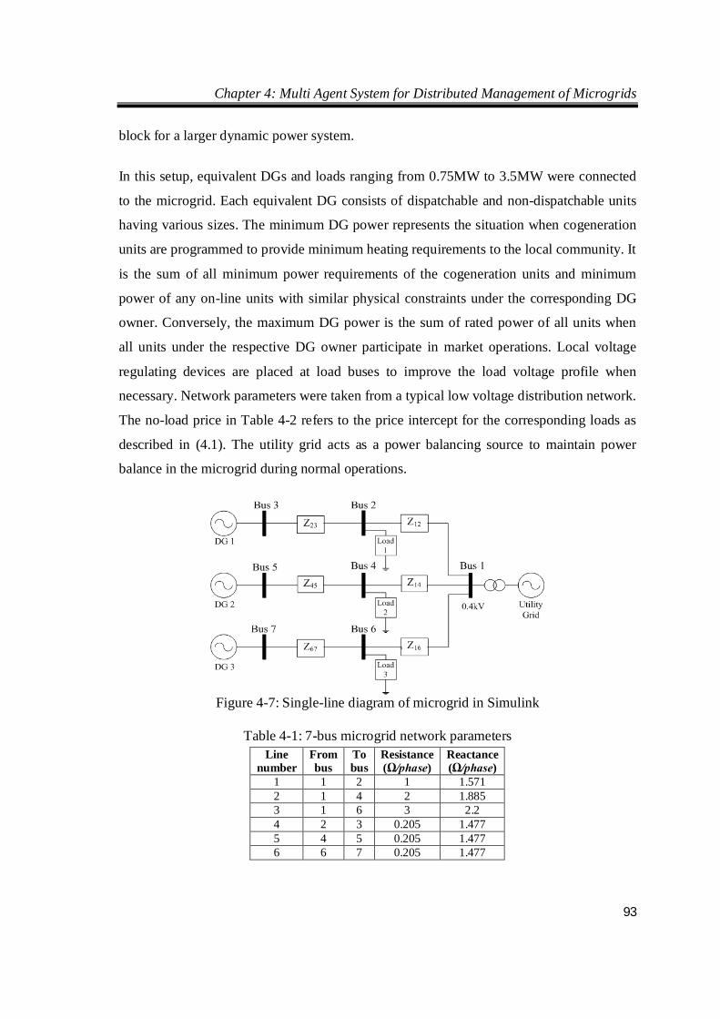
Chapter 4: Multi Agent System for Distributed Management of Microgrids
93
block for a larger dynamic power system.
In this setup, equivalent DGs and loads ranging from 0.75MW to 3.5MW were connected
to the microgrid. Each equivalent DG consists of dispatchable and non-dispatchable units
having various sizes. The minimum DG power represents the situation when cogeneration
units are programmed to provide minimum heating requirements to the local community. It
is the sum of all minimum power requirements of the cogeneration units and minimum
power of any on-line units with similar physical constraints under the corresponding DG
owner. Conversely, the maximum DG power is the sum of rated power of all units when
all units under the respective DG owner participate in market operations. Local voltage
regulating devices are placed at load buses to improve the load voltage profile when
necessary. Network parameters were taken from a typical low voltage distribution network.
The no-load price in Table 4-2 refers to the price intercept for the corresponding loads as
described in (4.1). The utility grid acts as a power balancing source to maintain power
balance in the microgrid during normal operations.
Figure 4-7: Single-line diagram of microgrid in Simulink
Table 4-1: 7-bus microgrid network parameters Line
number From bus
To bus
Resistance (Ω/phase)
Reactance (Ω/phase)
1 1 2 1 1.571 2 1 4 2 1.885 3 1 6 3 2.2 4 2 3 0.205 1.477 5 4 5 0.205 1.477 6 6 7 0.205 1.477
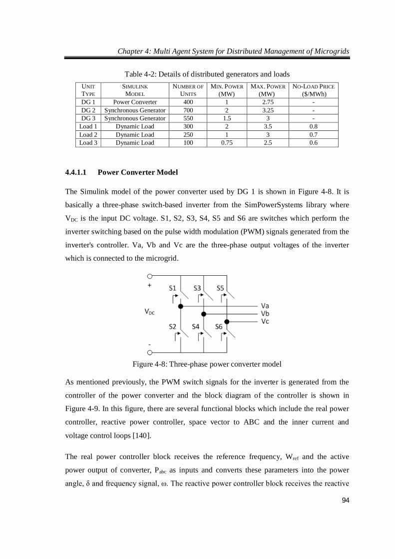
Chapter 4: Multi Agent System for Distributed Management of Microgrids
94
Table 4-2: Details of distributed generators and loads
4.4.1.1 Power Converter Model
The Simulink model of the power converter used by DG 1 is shown in Figure 4-8. It is
basically a three-phase switch-based inverter from the SimPowerSystems library where
VDC is the input DC voltage. S1, S2, S3, S4, S5 and S6 are switches which perform the
inverter switching based on the pulse width modulation (PWM) signals generated from the
inverter's controller. Va, Vb and Vc are the three-phase output voltages of the inverter
which is connected to the microgrid.
Figure 4-8: Three-phase power converter model
As mentioned previously, the PWM switch signals for the inverter is generated from the
controller of the power converter and the block diagram of the controller is shown in
Figure 4-9. In this figure, there are several functional blocks which include the real power
controller, reactive power controller, space vector to ABC and the inner current and
voltage control loops [140].
The real power controller block receives the reference frequency, Wref and the active
power output of converter, Pabc as inputs and converts these parameters into the power
angle, δ and frequency signal, ω. The reactive power controller block receives the reactive
UNIT TYPE
SIMULINK MODEL
NUMBER OF UNITS
MIN. POWER (MW)
MAX. POWER (MW)
NO-LOAD PRICE ($/MWh)
DG 1 Power Converter 400 1 2.75 - DG 2 Synchronous Generator 700 2 3.25 - DG 3 Synchronous Generator 550 1.5 3 -
Load 1 Dynamic Load 300 2 3.5 0.8 Load 2 Dynamic Load 250 1 3 0.7 Load 3 Dynamic Load 100 0.75 2.5 0.6
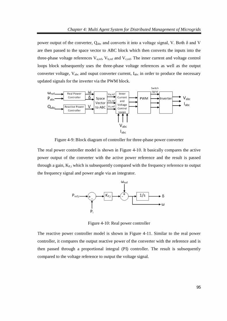
Chapter 4: Multi Agent System for Distributed Management of Microgrids
95
power output of the converter, Qabc and converts it into a voltage signal, V. Both δ and V
are then passed to the space vector to ABC block which then converts the inputs into the
three-phase voltage references Va,ref, Vb,ref and Vc,ref. The inner current and voltage control
loops block subsequently uses the three-phase voltage references as well as the output
converter voltage, Vabc and ouput converter current, Iabc in order to produce the necessary
updated signals for the inverter via the PWM block.
Figure 4-9: Block diagram of controller for three-phase power converter
The real power controller model is shown in Figure 4-10. It basically compares the active
power output of the converter with the active power reference and the result is passed
through a gain, KP,i which is subsequently compared with the frequency reference to output
the frequency signal and power angle via an integrator.
Figure 4-10: Real power controller
The reactive power controller model is shown in Figure 4-11. Similar to the real power
controller, it compares the output reactive power of the converter with the reference and is
then passed through a proportional integral (PI) controller. The result is subsequently
compared to the voltage reference to output the voltage signal.
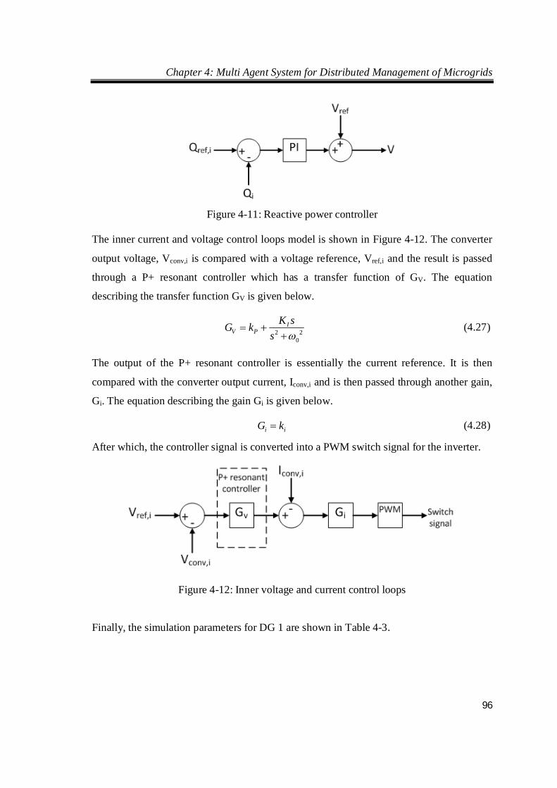
Chapter 4: Multi Agent System for Distributed Management of Microgrids
96
Figure 4-11: Reactive power controller
The inner current and voltage control loops model is shown in Figure 4-12. The converter
output voltage, Vconv,i is compared with a voltage reference, Vref,i and the result is passed
through a P+ resonant controller which has a transfer function of GV. The equation
describing the transfer function GV is given below.
2 20
IV P
K sG ks
(4.27)
The output of the P+ resonant controller is essentially the current reference. It is then
compared with the converter output current, Iconv,i and is then passed through another gain,
Gi. The equation describing the gain Gi is given below.
i iG k (4.28)
After which, the controller signal is converted into a PWM switch signal for the inverter.
Figure 4-12: Inner voltage and current control loops
Finally, the simulation parameters for DG 1 are shown in Table 4-3.
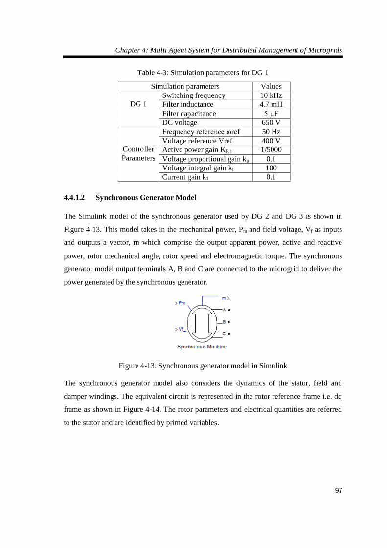
Chapter 4: Multi Agent System for Distributed Management of Microgrids
97
Table 4-3: Simulation parameters for DG 1
Simulation parameters Values
DG 1 Switching frequency 10 kHz Filter inductance 4.7 mH Filter capacitance 5 µF DC voltage 650 V
Controller Parameters
Frequency reference ωref 50 Hz Voltage reference Vref 400 V Active power gain KP,1 1/5000 Voltage proportional gain kp 0.1 Voltage integral gain kI 100 Current gain k1 0.1
4.4.1.2 Synchronous Generator Model
The Simulink model of the synchronous generator used by DG 2 and DG 3 is shown in
Figure 4-13. This model takes in the mechanical power, Pm and field voltage, Vf as inputs
and outputs a vector, m which comprise the output apparent power, active and reactive
power, rotor mechanical angle, rotor speed and electromagnetic torque. The synchronous
generator model output terminals A, B and C are connected to the microgrid to deliver the
power generated by the synchronous generator.
Figure 4-13: Synchronous generator model in Simulink
The synchronous generator model also considers the dynamics of the stator, field and
damper windings. The equivalent circuit is represented in the rotor reference frame i.e. dq
frame as shown in Figure 4-14. The rotor parameters and electrical quantities are referred
to the stator and are identified by primed variables.
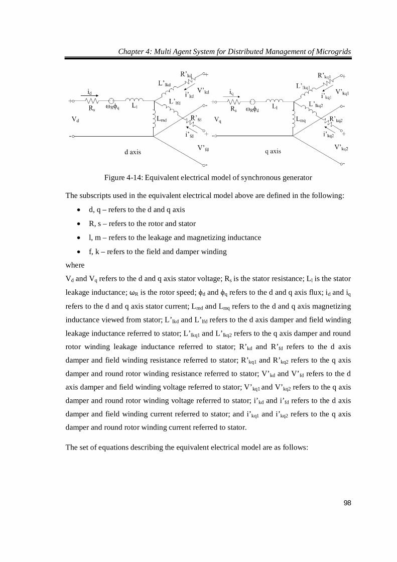
Chapter 4: Multi Agent System for Distributed Management of Microgrids
98
Figure 4-14: Equivalent electrical model of synchronous generator
The subscripts used in the equivalent electrical model above are defined in the following:
d, q – refers to the d and q axis
R, s – refers to the rotor and stator
l, m – refers to the leakage and magnetizing inductance
f, k – refers to the field and damper winding
where
Vd and Vq refers to the d and q axis stator voltage; Rs is the stator resistance; Ll is the stator
leakage inductance; ωR is the rotor speed; ϕd and ϕq refers to the d and q axis flux; id and iq
refers to the d and q axis stator current; Lmd and Lmq refers to the d and q axis magnetizing
inductance viewed from stator; L’lkd and L’lfd refers to the d axis damper and field winding
leakage inductance referred to stator; L’lkq1 and L’lkq2 refers to the q axis damper and round
rotor winding leakage inductance referred to stator; R’kd and R’fd refers to the d axis
damper and field winding resistance referred to stator; R’kq1 and R’kq2 refers to the q axis
damper and round rotor winding resistance referred to stator; V’kd and V’fd refers to the d
axis damper and field winding voltage referred to stator; V’kq1 and V’kq2 refers to the q axis
damper and round rotor winding voltage referred to stator; i’kd and i’fd refers to the d axis
damper and field winding current referred to stator; and i’kq1 and i’kq2 refers to the q axis
damper and round rotor winding current referred to stator.
The set of equations describing the equivalent electrical model are as follows:
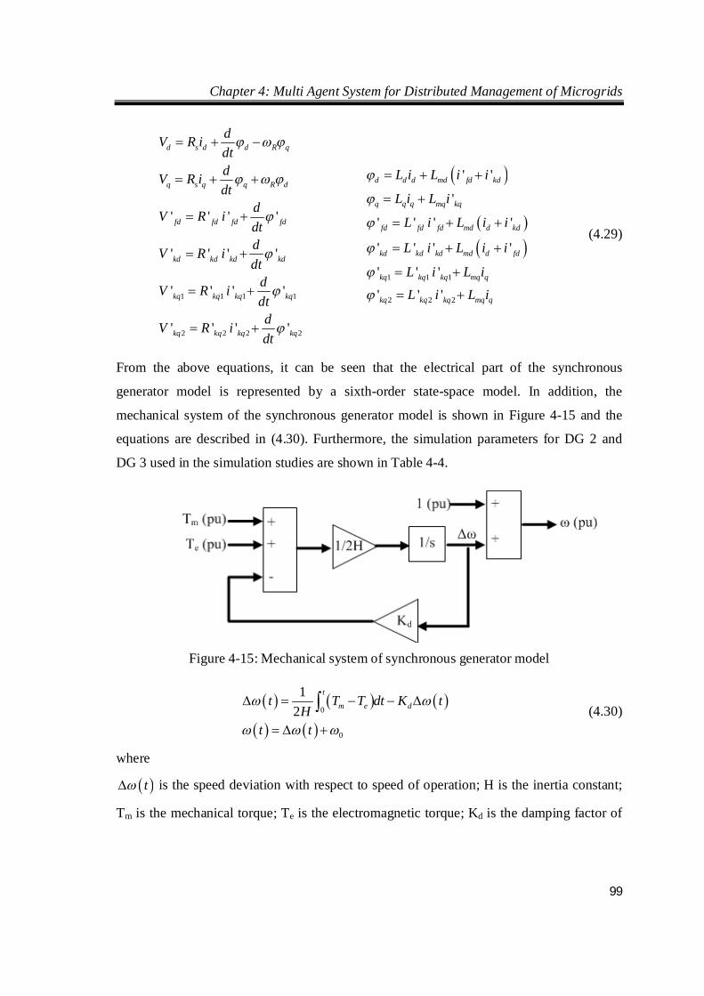
Chapter 4: Multi Agent System for Distributed Management of Microgrids
99
1 1 1 1
2 2 2 2
' ' ' '
' ' ' '
' ' ' '
' ' ' '
d s d d R q
q s q q R d
fd fd fd fd
kd kd kd kd
kq kq kq kq
kq kq kq kq
dV R idtdV R idt
dV R idtdV R idt
dV R idtdV R idt
1 1 1
2 2 2
' '
'
' ' ' '
' ' ' '
' ' '
' ' '
d d d md fd kd
q q q mq kq
fd fd fd md d kd
kd kd kd md d fd
kq kq kq mq q
kq kq kq mq q
L i L i i
L i L i
L i L i i
L i L i i
L i L iL i L i
(4.29)
From the above equations, it can be seen that the electrical part of the synchronous
generator model is represented by a sixth-order state-space model. In addition, the
mechanical system of the synchronous generator model is shown in Figure 4-15 and the
equations are described in (4.30). Furthermore, the simulation parameters for DG 2 and
DG 3 used in the simulation studies are shown in Table 4-4.
Figure 4-15: Mechanical system of synchronous generator model
0
0
12
t
m e dt T T dt K tH
t t
(4.30)
where
t is the speed deviation with respect to speed of operation; H is the inertia constant;
Tm is the mechanical torque; Te is the electromagnetic torque; Kd is the damping factor of
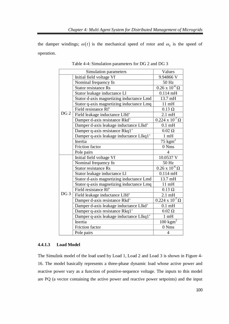
Chapter 4: Multi Agent System for Distributed Management of Microgrids
100
the damper windings; t is the mechanical speed of rotor and 0 is the speed of
operation.
Table 4-4: Simulation parameters for DG 2 and DG 3
Simulation parameters Values
DG 2
Initial field voltage Vf 9.94866 V Nominal frequency fn 50 Hz Stator resistance Rs 0.26 x 10⁻⁶ Ω
Stator leakage inductance Ll 0.114 mH Stator d-axis magnetizing inductance Lmd 13.7 mH Stator q-axis magnetizing inductance Lmq 11 mH Field resistance Rf’ 0.13 Ω Field leakage inductance Llfd’ 2.1 mH Damper d-axis resistance Rkd’ 0.224 x 10⁻⁷ Ω Damper d-axis leakage inductance Llkd’ 0.1 mH Damper q-axis resistance Rkq1’ 0.02 Ω Damper q-axis leakage inductance Llkq1’ 1 mH Inertia 75 kgm2 Friction factor 0 Nms Pole pairs 4
DG 3
Initial field voltage Vf 10.0537 V Nominal frequency fn 50 Hz Stator resistance Rs 0.26 x 10⁻⁶ Ω
Stator leakage inductance Ll 0.114 mH Stator d-axis magnetizing inductance Lmd 13.7 mH Stator q-axis magnetizing inductance Lmq 11 mH Field resistance Rf’ 0.13 Ω Field leakage inductance Llfd’ 2.1 mH Damper d-axis resistance Rkd’ 0.224 x 10⁻⁷ Ω Damper d-axis leakage inductance Llkd’ 0.1 mH Damper q-axis resistance Rkq1’ 0.02 Ω Damper q-axis leakage inductance Llkq1’ 1 mH Inertia 100 kgm2 Friction factor 0 Nms Pole pairs 4
4.4.1.3 Load Model
The Simulink model of the load used by Load 1, Load 2 and Load 3 is shown in Figure 4-
16. The model basically represents a three-phase dynamic load whose active power and
reactive power vary as a function of positive-sequence voltage. The inputs to this model
are PQ (a vector containing the active power and reactive power setpoints) and the input
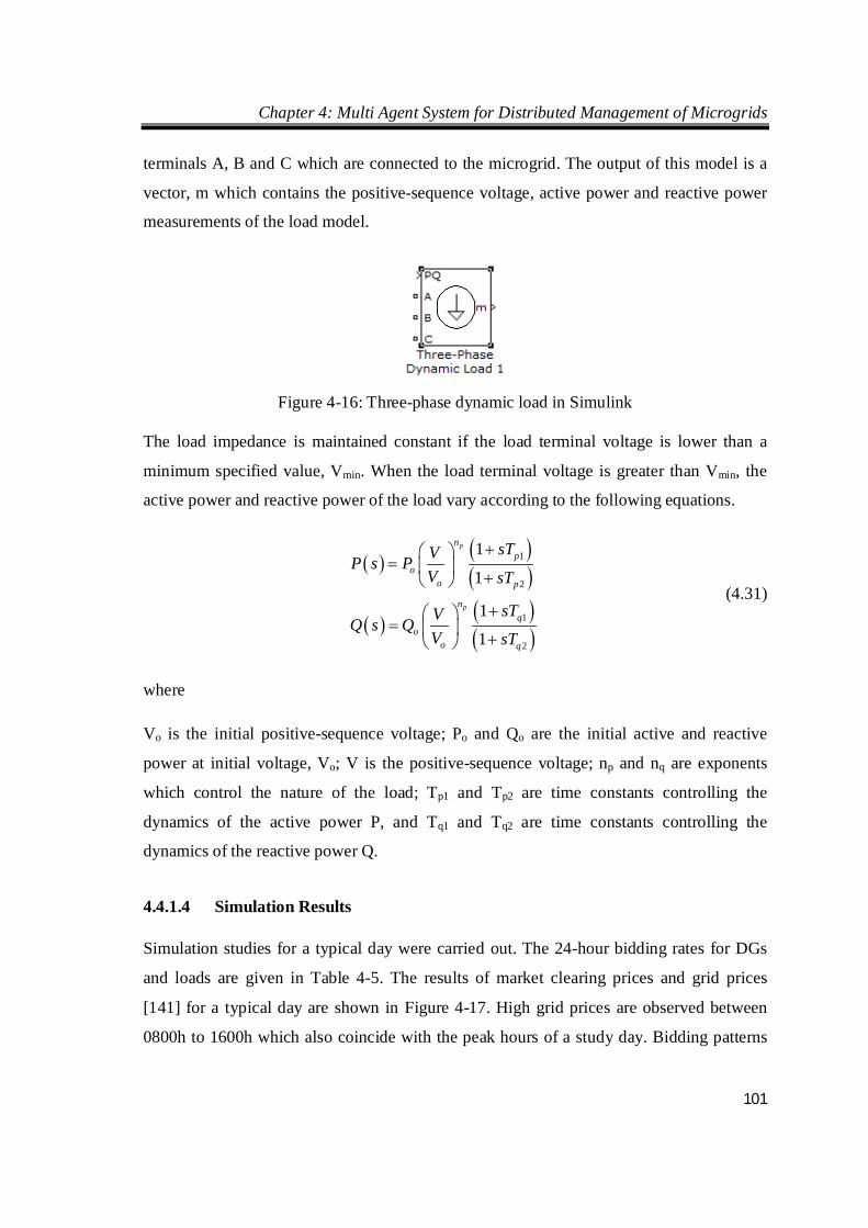
Chapter 4: Multi Agent System for Distributed Management of Microgrids
101
terminals A, B and C which are connected to the microgrid. The output of this model is a
vector, m which contains the positive-sequence voltage, active power and reactive power
measurements of the load model.
Figure 4-16: Three-phase dynamic load in Simulink
The load impedance is maintained constant if the load terminal voltage is lower than a
minimum specified value, Vmin. When the load terminal voltage is greater than Vmin, the
active power and reactive power of the load vary according to the following equations.
1
2
1
2
1
1
1
1
p
p
np
oo p
nq
oo q
sTVP s PV sT
sTVQ s QV sT
(4.31)
where
Vo is the initial positive-sequence voltage; Po and Qo are the initial active and reactive
power at initial voltage, Vo; V is the positive-sequence voltage; np and nq are exponents
which control the nature of the load; Tp1 and Tp2 are time constants controlling the
dynamics of the active power P, and Tq1 and Tq2 are time constants controlling the
dynamics of the reactive power Q.
4.4.1.4 Simulation Results
Simulation studies for a typical day were carried out. The 24-hour bidding rates for DGs
and loads are given in Table 4-5. The results of market clearing prices and grid prices
[141] for a typical day are shown in Figure 4-17. High grid prices are observed between
0800h to 1600h which also coincide with the peak hours of a study day. Bidding patterns
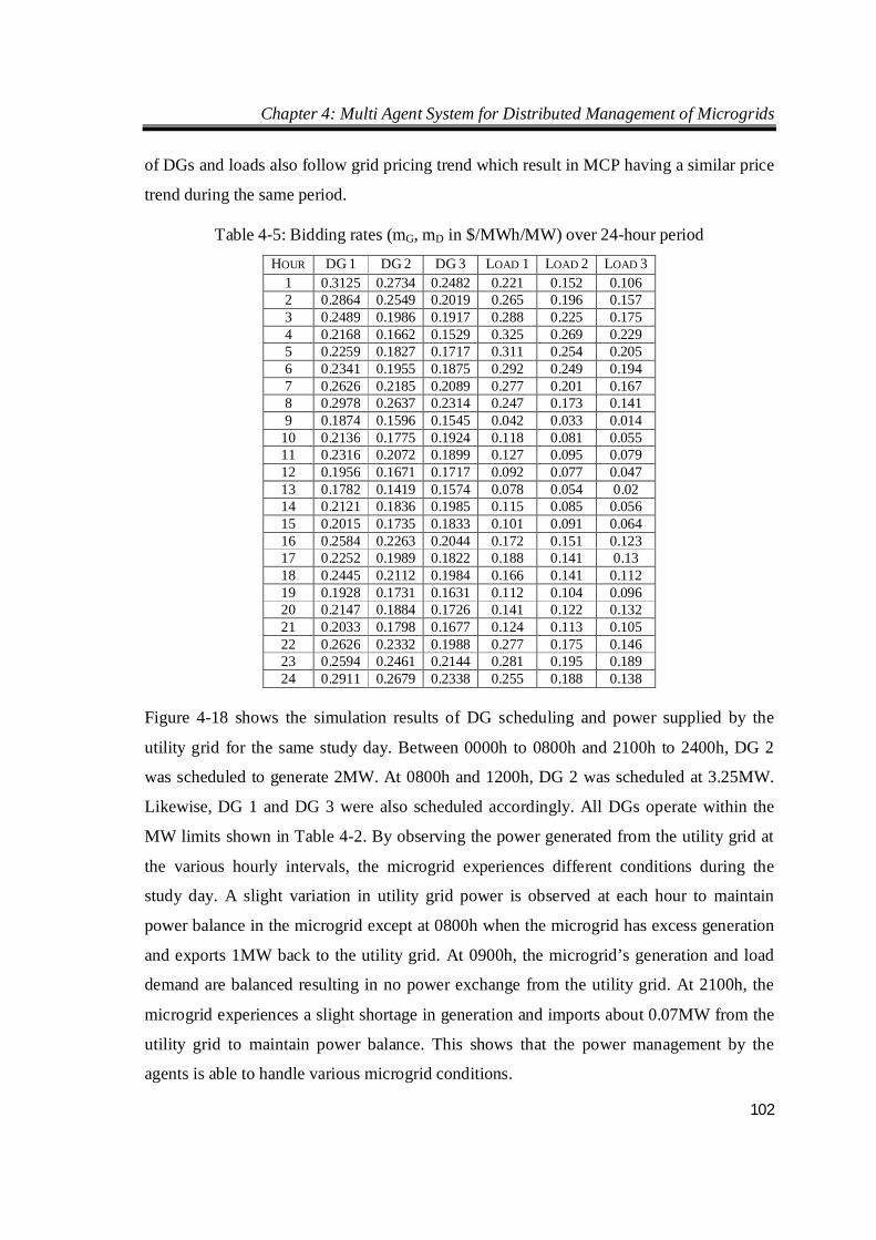
Chapter 4: Multi Agent System for Distributed Management of Microgrids
102
of DGs and loads also follow grid pricing trend which result in MCP having a similar price
trend during the same period.
Table 4-5: Bidding rates (mG, mD in $/MWh/MW) over 24-hour period
HOUR DG 1 DG 2 DG 3 LOAD 1 LOAD 2 LOAD 3 1 0.3125 0.2734 0.2482 0.221 0.152 0.106 2 0.2864 0.2549 0.2019 0.265 0.196 0.157 3 0.2489 0.1986 0.1917 0.288 0.225 0.175 4 0.2168 0.1662 0.1529 0.325 0.269 0.229 5 0.2259 0.1827 0.1717 0.311 0.254 0.205 6 0.2341 0.1955 0.1875 0.292 0.249 0.194 7 0.2626 0.2185 0.2089 0.277 0.201 0.167 8 0.2978 0.2637 0.2314 0.247 0.173 0.141 9 0.1874 0.1596 0.1545 0.042 0.033 0.014
10 0.2136 0.1775 0.1924 0.118 0.081 0.055 11 0.2316 0.2072 0.1899 0.127 0.095 0.079 12 0.1956 0.1671 0.1717 0.092 0.077 0.047 13 0.1782 0.1419 0.1574 0.078 0.054 0.02 14 0.2121 0.1836 0.1985 0.115 0.085 0.056 15 0.2015 0.1735 0.1833 0.101 0.091 0.064 16 0.2584 0.2263 0.2044 0.172 0.151 0.123 17 0.2252 0.1989 0.1822 0.188 0.141 0.13 18 0.2445 0.2112 0.1984 0.166 0.141 0.112 19 0.1928 0.1731 0.1631 0.112 0.104 0.096 20 0.2147 0.1884 0.1726 0.141 0.122 0.132 21 0.2033 0.1798 0.1677 0.124 0.113 0.105 22 0.2626 0.2332 0.1988 0.277 0.175 0.146 23 0.2594 0.2461 0.2144 0.281 0.195 0.189 24 0.2911 0.2679 0.2338 0.255 0.188 0.138
Figure 4-18 shows the simulation results of DG scheduling and power supplied by the
utility grid for the same study day. Between 0000h to 0800h and 2100h to 2400h, DG 2
was scheduled to generate 2MW. At 0800h and 1200h, DG 2 was scheduled at 3.25MW.
Likewise, DG 1 and DG 3 were also scheduled accordingly. All DGs operate within the
MW limits shown in Table 4-2. By observing the power generated from the utility grid at
the various hourly intervals, the microgrid experiences different conditions during the
study day. A slight variation in utility grid power is observed at each hour to maintain
power balance in the microgrid except at 0800h when the microgrid has excess generation
and exports 1MW back to the utility grid. At 0900h, the microgrid’s generation and load
demand are balanced resulting in no power exchange from the utility grid. At 2100h, the
microgrid experiences a slight shortage in generation and imports about 0.07MW from the
utility grid to maintain power balance. This shows that the power management by the
agents is able to handle various microgrid conditions.
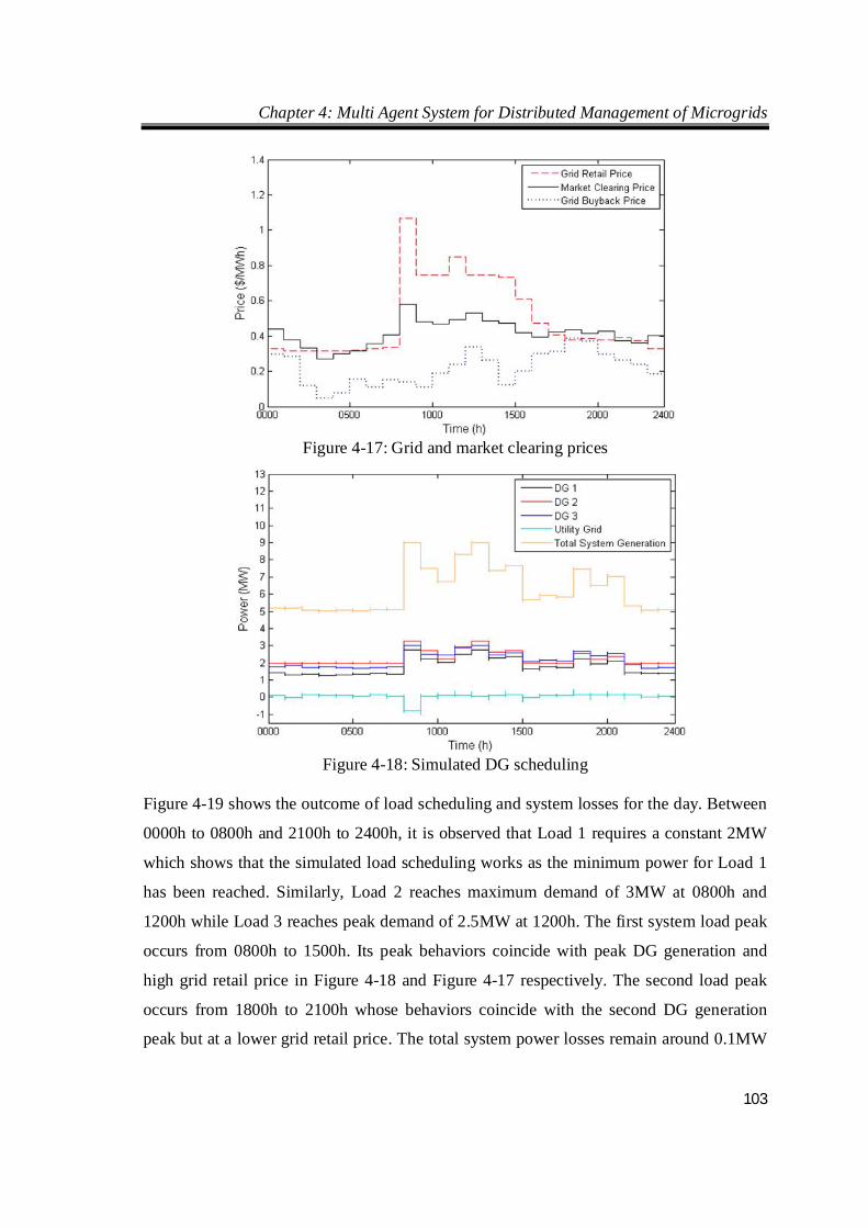
Chapter 4: Multi Agent System for Distributed Management of Microgrids
103
Figure 4-17: Grid and market clearing prices
Figure 4-18: Simulated DG scheduling
Figure 4-19 shows the outcome of load scheduling and system losses for the day. Between
0000h to 0800h and 2100h to 2400h, it is observed that Load 1 requires a constant 2MW
which shows that the simulated load scheduling works as the minimum power for Load 1
has been reached. Similarly, Load 2 reaches maximum demand of 3MW at 0800h and
1200h while Load 3 reaches peak demand of 2.5MW at 1200h. The first system load peak
occurs from 0800h to 1500h. Its peak behaviors coincide with peak DG generation and
high grid retail price in Figure 4-18 and Figure 4-17 respectively. The second load peak
occurs from 1800h to 2100h whose behaviors coincide with the second DG generation
peak but at a lower grid retail price. The total system power losses remain around 0.1MW
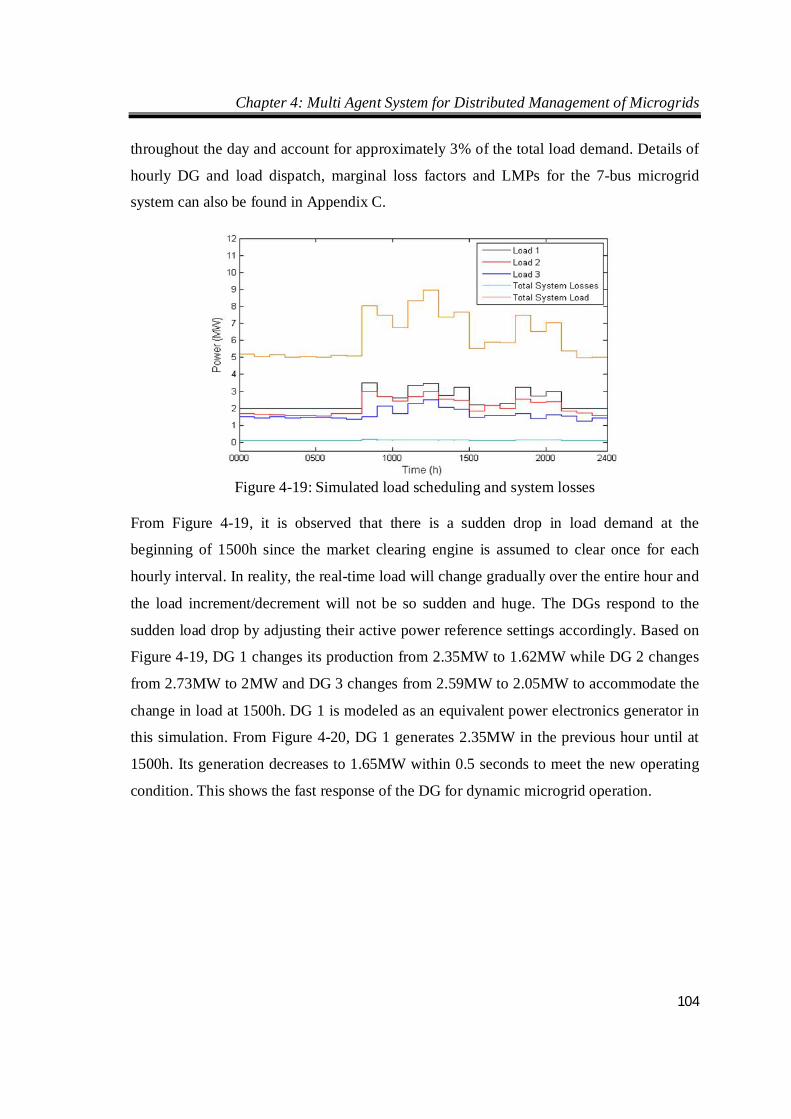
Chapter 4: Multi Agent System for Distributed Management of Microgrids
104
throughout the day and account for approximately 3% of the total load demand. Details of
hourly DG and load dispatch, marginal loss factors and LMPs for the 7-bus microgrid
system can also be found in Appendix C.
Figure 4-19: Simulated load scheduling and system losses
From Figure 4-19, it is observed that there is a sudden drop in load demand at the
beginning of 1500h since the market clearing engine is assumed to clear once for each
hourly interval. In reality, the real-time load will change gradually over the entire hour and
the load increment/decrement will not be so sudden and huge. The DGs respond to the
sudden load drop by adjusting their active power reference settings accordingly. Based on
Figure 4-19, DG 1 changes its production from 2.35MW to 1.62MW while DG 2 changes
from 2.73MW to 2MW and DG 3 changes from 2.59MW to 2.05MW to accommodate the
change in load at 1500h. DG 1 is modeled as an equivalent power electronics generator in
this simulation. From Figure 4-20, DG 1 generates 2.35MW in the previous hour until at
1500h. Its generation decreases to 1.65MW within 0.5 seconds to meet the new operating
condition. This shows the fast response of the DG for dynamic microgrid operation.
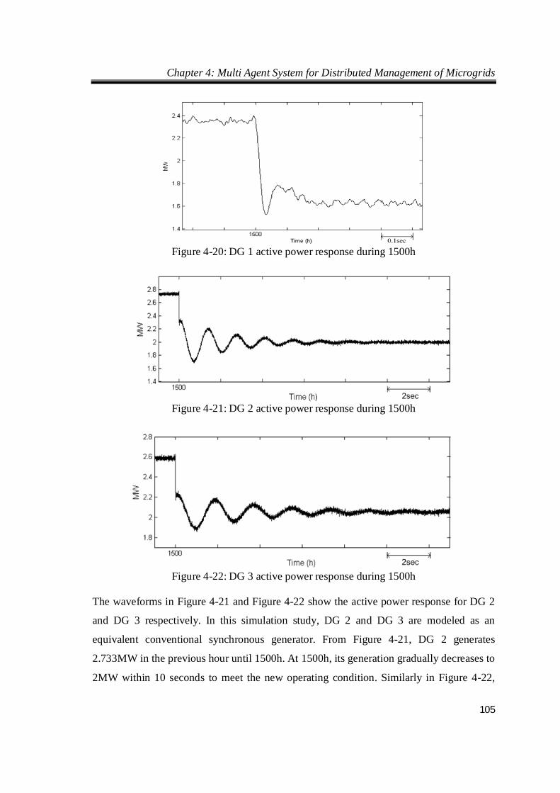
Chapter 4: Multi Agent System for Distributed Management of Microgrids
105
Figure 4-20: DG 1 active power response during 1500h
Figure 4-21: DG 2 active power response during 1500h
Figure 4-22: DG 3 active power response during 1500h
The waveforms in Figure 4-21 and Figure 4-22 show the active power response for DG 2
and DG 3 respectively. In this simulation study, DG 2 and DG 3 are modeled as an
equivalent conventional synchronous generator. From Figure 4-21, DG 2 generates
2.733MW in the previous hour until 1500h. At 1500h, its generation gradually decreases to
2MW within 10 seconds to meet the new operating condition. Similarly in Figure 4-22,
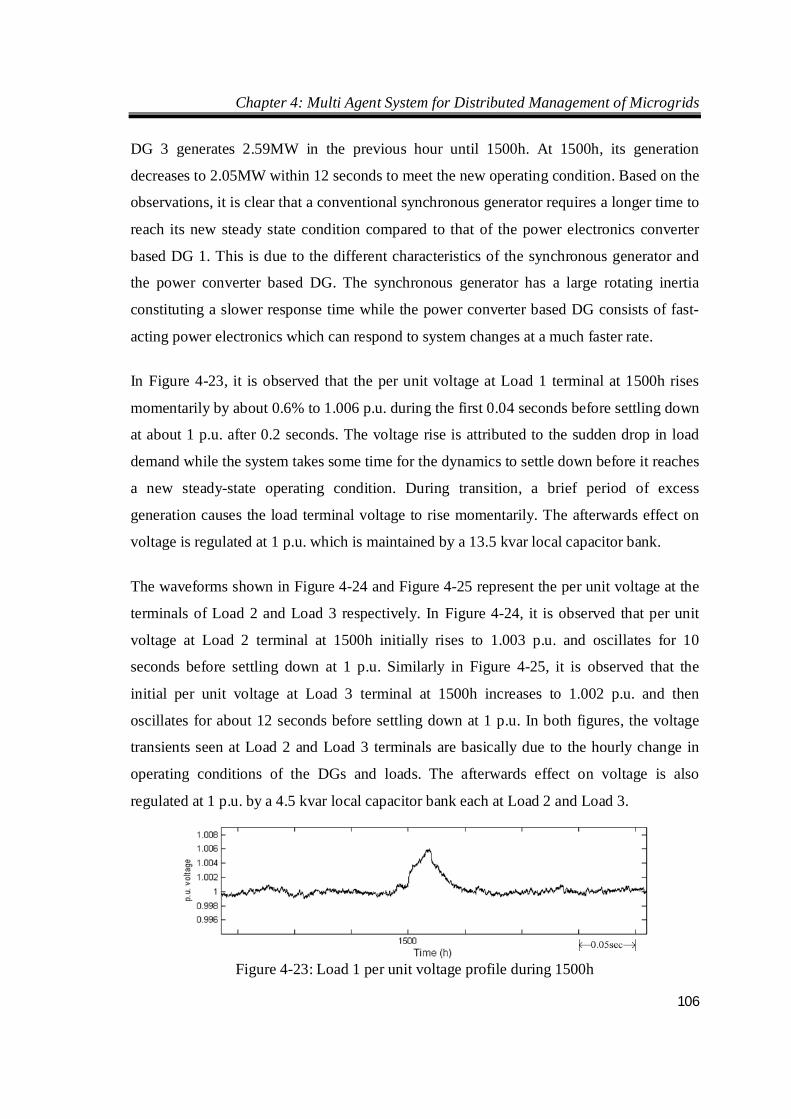
Chapter 4: Multi Agent System for Distributed Management of Microgrids
106
DG 3 generates 2.59MW in the previous hour until 1500h. At 1500h, its generation
decreases to 2.05MW within 12 seconds to meet the new operating condition. Based on the
observations, it is clear that a conventional synchronous generator requires a longer time to
reach its new steady state condition compared to that of the power electronics converter
based DG 1. This is due to the different characteristics of the synchronous generator and
the power converter based DG. The synchronous generator has a large rotating inertia
constituting a slower response time while the power converter based DG consists of fast-
acting power electronics which can respond to system changes at a much faster rate.
In Figure 4-23, it is observed that the per unit voltage at Load 1 terminal at 1500h rises
momentarily by about 0.6% to 1.006 p.u. during the first 0.04 seconds before settling down
at about 1 p.u. after 0.2 seconds. The voltage rise is attributed to the sudden drop in load
demand while the system takes some time for the dynamics to settle down before it reaches
a new steady-state operating condition. During transition, a brief period of excess
generation causes the load terminal voltage to rise momentarily. The afterwards effect on
voltage is regulated at 1 p.u. which is maintained by a 13.5 kvar local capacitor bank.
The waveforms shown in Figure 4-24 and Figure 4-25 represent the per unit voltage at the
terminals of Load 2 and Load 3 respectively. In Figure 4-24, it is observed that per unit
voltage at Load 2 terminal at 1500h initially rises to 1.003 p.u. and oscillates for 10
seconds before settling down at 1 p.u. Similarly in Figure 4-25, it is observed that the
initial per unit voltage at Load 3 terminal at 1500h increases to 1.002 p.u. and then
oscillates for about 12 seconds before settling down at 1 p.u. In both figures, the voltage
transients seen at Load 2 and Load 3 terminals are basically due to the hourly change in
operating conditions of the DGs and loads. The afterwards effect on voltage is also
regulated at 1 p.u. by a 4.5 kvar local capacitor bank each at Load 2 and Load 3.
Figure 4-23: Load 1 per unit voltage profile during 1500h
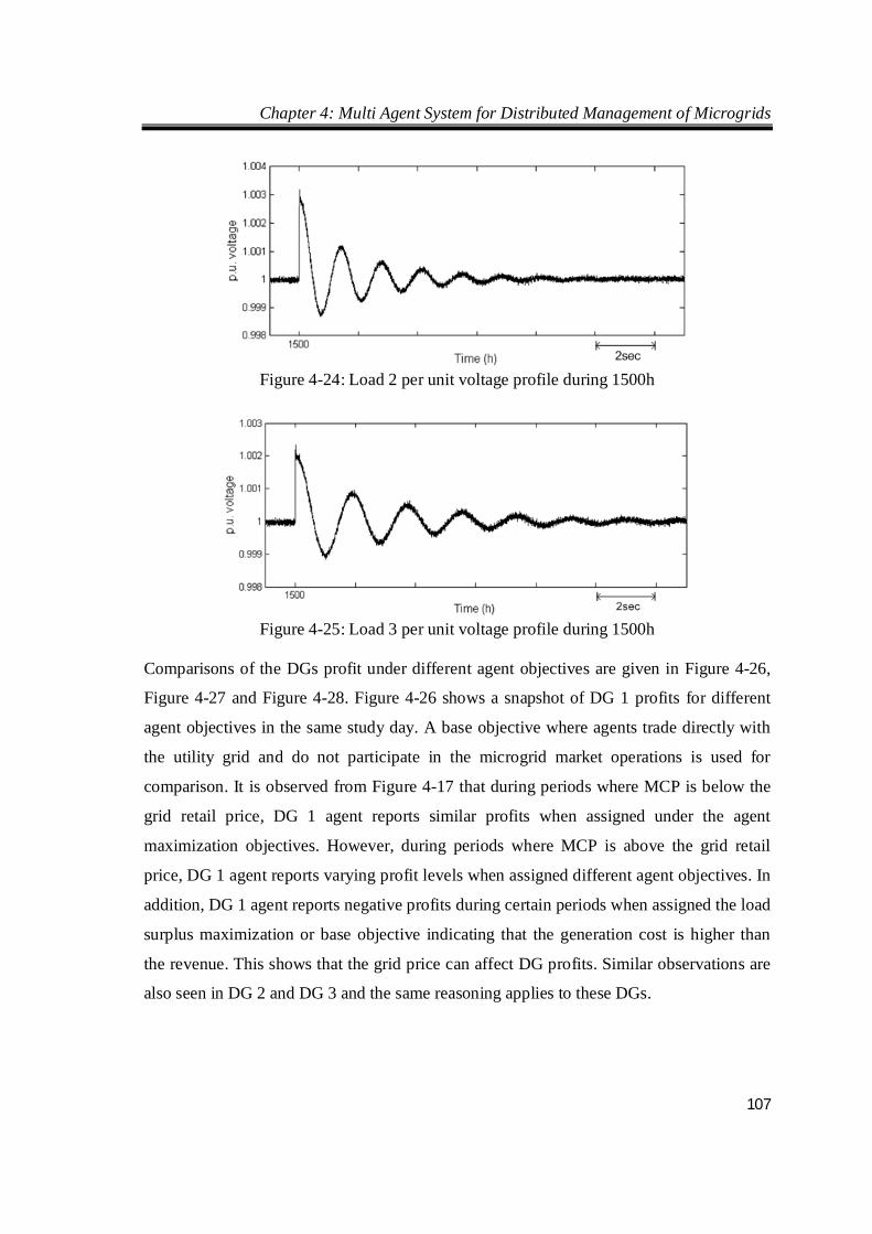
Chapter 4: Multi Agent System for Distributed Management of Microgrids
107
Figure 4-24: Load 2 per unit voltage profile during 1500h
Figure 4-25: Load 3 per unit voltage profile during 1500h
Comparisons of the DGs profit under different agent objectives are given in Figure 4-26,
Figure 4-27 and Figure 4-28. Figure 4-26 shows a snapshot of DG 1 profits for different
agent objectives in the same study day. A base objective where agents trade directly with
the utility grid and do not participate in the microgrid market operations is used for
comparison. It is observed from Figure 4-17 that during periods where MCP is below the
grid retail price, DG 1 agent reports similar profits when assigned under the agent
maximization objectives. However, during periods where MCP is above the grid retail
price, DG 1 agent reports varying profit levels when assigned different agent objectives. In
addition, DG 1 agent reports negative profits during certain periods when assigned the load
surplus maximization or base objective indicating that the generation cost is higher than
the revenue. This shows that the grid price can affect DG profits. Similar observations are
also seen in DG 2 and DG 3 and the same reasoning applies to these DGs.
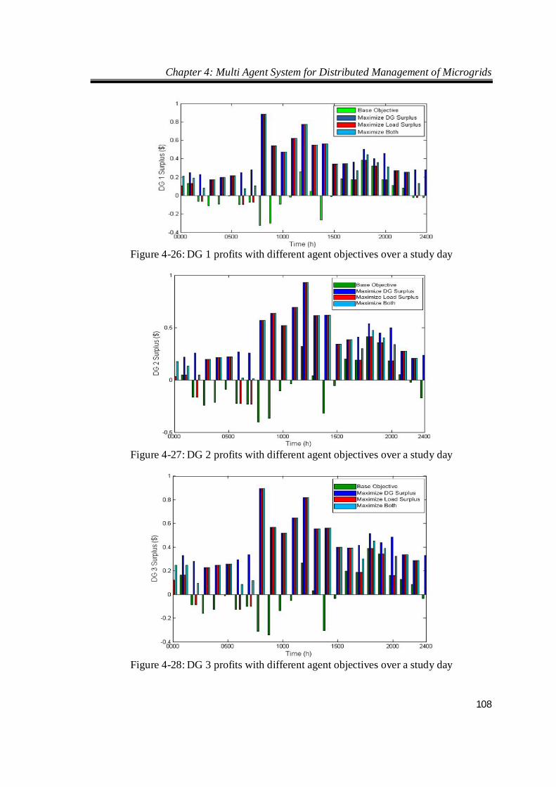
Chapter 4: Multi Agent System for Distributed Management of Microgrids
108
Figure 4-26: DG 1 profits with different agent objectives over a study day
Figure 4-27: DG 2 profits with different agent objectives over a study day
Figure 4-28: DG 3 profits with different agent objectives over a study day
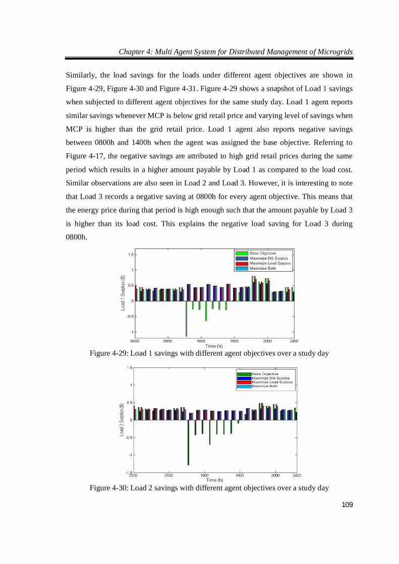
Chapter 4: Multi Agent System for Distributed Management of Microgrids
109
Similarly, the load savings for the loads under different agent objectives are shown in
Figure 4-29, Figure 4-30 and Figure 4-31. Figure 4-29 shows a snapshot of Load 1 savings
when subjected to different agent objectives for the same study day. Load 1 agent reports
similar savings whenever MCP is below grid retail price and varying level of savings when
MCP is higher than the grid retail price. Load 1 agent also reports negative savings
between 0800h and 1400h when the agent was assigned the base objective. Referring to
Figure 4-17, the negative savings are attributed to high grid retail prices during the same
period which results in a higher amount payable by Load 1 as compared to the load cost.
Similar observations are also seen in Load 2 and Load 3. However, it is interesting to note
that Load 3 records a negative saving at 0800h for every agent objective. This means that
the energy price during that period is high enough such that the amount payable by Load 3
is higher than its load cost. This explains the negative load saving for Load 3 during
0800h.
Figure 4-29: Load 1 savings with different agent objectives over a study day
Figure 4-30: Load 2 savings with different agent objectives over a study day
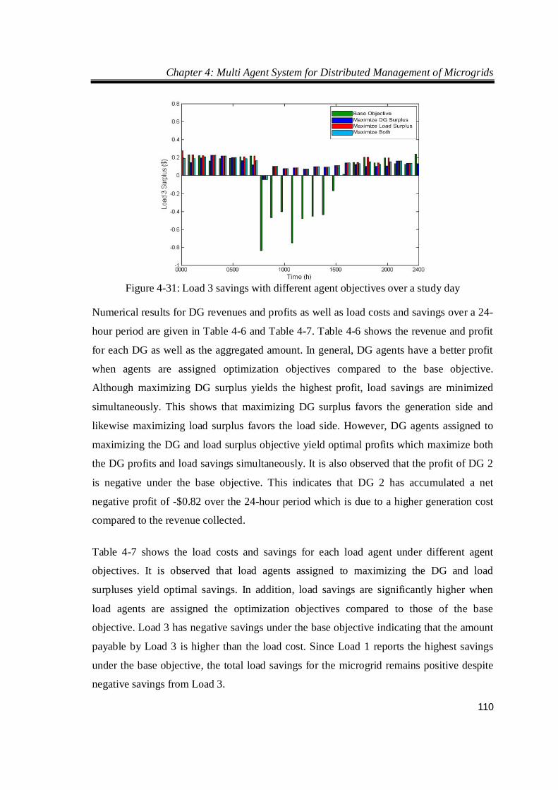
Chapter 4: Multi Agent System for Distributed Management of Microgrids
110
Figure 4-31: Load 3 savings with different agent objectives over a study day
Numerical results for DG revenues and profits as well as load costs and savings over a 24-
hour period are given in Table 4-6 and Table 4-7. Table 4-6 shows the revenue and profit
for each DG as well as the aggregated amount. In general, DG agents have a better profit
when agents are assigned optimization objectives compared to the base objective.
Although maximizing DG surplus yields the highest profit, load savings are minimized
simultaneously. This shows that maximizing DG surplus favors the generation side and
likewise maximizing load surplus favors the load side. However, DG agents assigned to
maximizing the DG and load surplus objective yield optimal profits which maximize both
the DG profits and load savings simultaneously. It is also observed that the profit of DG 2
is negative under the base objective. This indicates that DG 2 has accumulated a net
negative profit of -$0.82 over the 24-hour period which is due to a higher generation cost
compared to the revenue collected.
Table 4-7 shows the load costs and savings for each load agent under different agent
objectives. It is observed that load agents assigned to maximizing the DG and load
surpluses yield optimal savings. In addition, load savings are significantly higher when
load agents are assigned the optimization objectives compared to those of the base
objective. Load 3 has negative savings under the base objective indicating that the amount
payable by Load 3 is higher than the load cost. Since Load 1 reports the highest savings
under the base objective, the total load savings for the microgrid remains positive despite
negative savings from Load 3.
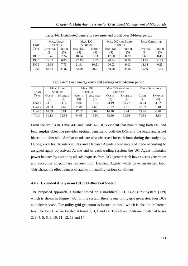
Chapter 4: Multi Agent System for Distributed Management of Microgrids
111
Table 4-6: Distributed generators revenue and profit over 24-hour period
UNIT TYPE
MAX. LOAD SURPLUS
MAX. DG SURPLUS
MAX DG AND LOAD SURPLUS
BASE OBJECTIVE
REVENUE ($)
PROFIT ($)
REVENUE ($)
PROFIT ($)
REVENUE ($)
PROFIT ($)
REVENUE ($)
PROFIT ($)
DG 1 16.45 7.24 18.74 9.53 17.60 8.39 9.69 0.48 DG 2 19.43 6.85 22.45 9.87 20.94 8.36 11.76 -0.82 DG 3 18.63 7.73 21.41 10.51 20.02 9.12 11.14 0.25 Total 54.51 21.82 62.60 29.91 58.56 25.87 32.59 -0.09
Table 4-7: Load energy costs and savings over 24-hour period
LOAD TYPE
MAX. LOAD SURPLUS
MAX. DG SURPLUS
MAX DG AND LOAD SURPLUS
BASE OBJECTIVE
COSTS ($)
SAVINGS ($)
COSTS ($)
SAVINGS ($)
COSTS ($)
SAVINGS ($)
COSTS ($)
SAVINGS ($)
Load 1 23.91 11.36 25.07 10.19 24.49 10.77 31.24 4.02 Load 2 20.83 7.67 21.81 6.69 21.32 7.18 27.32 1.18 Load 3 16.39 3.81 17.17 3.02 16.78 3.41 21.26 -1.07 Total 61.13 22.84 64.05 19.90 62.59 21.36 79.82 4.13
From the results in Table 4-6 and Table 4-7, it is evident that maximizing both DG and
load surplus objective provides optimal benefits to both the DGs and the loads and is not
biased to either side. Similar trends are also observed for each hour during the study day.
During each hourly interval, DG and Demand Agents coordinate and trade according to
assigned agent objectives. At the end of each trading session, the UG Agent maintains
power balance by accepting all sale requests from DG agents which have excess generation
and accepting all purchase requests from Demand Agents which have unsatisfied load.
This shows the effectiveness of agents in handling various conditions.
4.4.2 Extended Analysis on IEEE 14-Bus Test System
The proposed approach is further tested on a modified IEEE 14-bus test system [139]
which is shown in Figure 4-32. In this system, there is one utility grid generator, four DGs
and eleven loads. The utility grid generator is located at bus 1 which is also the reference
bus. The four DGs are located at buses 2, 3, 4 and 12. The eleven loads are located at buses
2, 3, 4, 5, 6, 9, 10, 11, 12, 13 and 14.
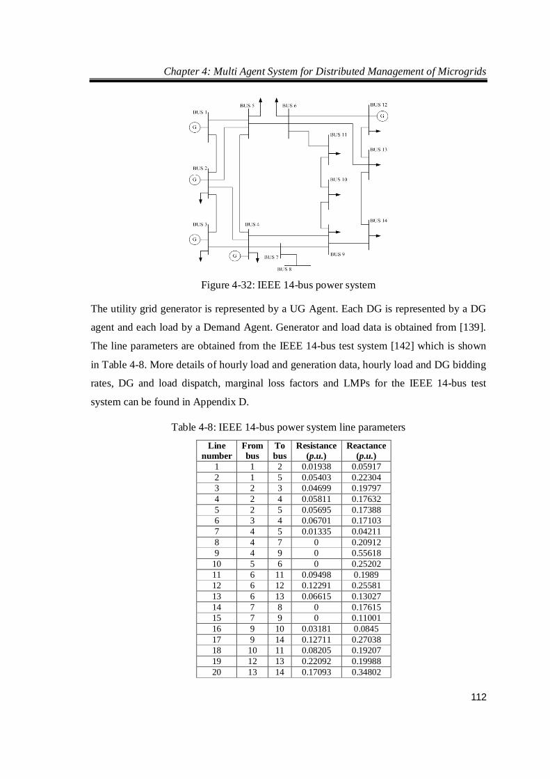
Chapter 4: Multi Agent System for Distributed Management of Microgrids
112
Figure 4-32: IEEE 14-bus power system
The utility grid generator is represented by a UG Agent. Each DG is represented by a DG
agent and each load by a Demand Agent. Generator and load data is obtained from [139].
The line parameters are obtained from the IEEE 14-bus test system [142] which is shown
in Table 4-8. More details of hourly load and generation data, hourly load and DG bidding
rates, DG and load dispatch, marginal loss factors and LMPs for the IEEE 14-bus test
system can be found in Appendix D.
Table 4-8: IEEE 14-bus power system line parameters
Line number
From bus
To bus
Resistance (p.u.)
Reactance (p.u.)
1 1 2 0.01938 0.05917 2 1 5 0.05403 0.22304 3 2 3 0.04699 0.19797 4 2 4 0.05811 0.17632 5 2 5 0.05695 0.17388 6 3 4 0.06701 0.17103 7 4 5 0.01335 0.04211 8 4 7 0 0.20912 9 4 9 0 0.55618
10 5 6 0 0.25202 11 6 11 0.09498 0.1989 12 6 12 0.12291 0.25581 13 6 13 0.06615 0.13027 14 7 8 0 0.17615 15 7 9 0 0.11001 16 9 10 0.03181 0.0845 17 9 14 0.12711 0.27038 18 10 11 0.08205 0.19207 19 12 13 0.22092 0.19988 20 13 14 0.17093 0.34802
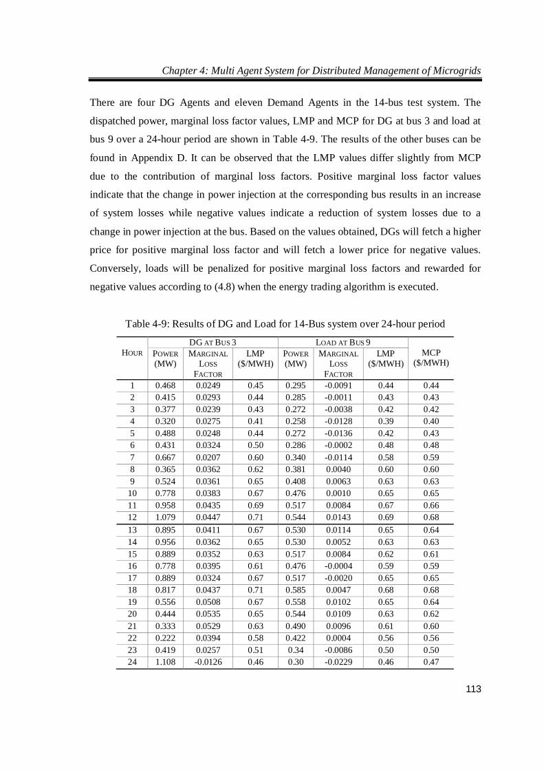
Chapter 4: Multi Agent System for Distributed Management of Microgrids
113
There are four DG Agents and eleven Demand Agents in the 14-bus test system. The
dispatched power, marginal loss factor values, LMP and MCP for DG at bus 3 and load at
bus 9 over a 24-hour period are shown in Table 4-9. The results of the other buses can be
found in Appendix D. It can be observed that the LMP values differ slightly from MCP
due to the contribution of marginal loss factors. Positive marginal loss factor values
indicate that the change in power injection at the corresponding bus results in an increase
of system losses while negative values indicate a reduction of system losses due to a
change in power injection at the bus. Based on the values obtained, DGs will fetch a higher
price for positive marginal loss factor and will fetch a lower price for negative values.
Conversely, loads will be penalized for positive marginal loss factors and rewarded for
negative values according to (4.8) when the energy trading algorithm is executed.
Table 4-9: Results of DG and Load for 14-Bus system over 24-hour period
HOUR
DG AT BUS 3 LOAD AT BUS 9 MCP
($/MWH) POWER (MW)
MARGINAL LOSS
FACTOR
LMP ($/MWH)
POWER (MW)
MARGINAL LOSS
FACTOR
LMP ($/MWH)
1 0.468 0.0249 0.45 0.295 -0.0091 0.44 0.44 2 0.415 0.0293 0.44 0.285 -0.0011 0.43 0.43 3 0.377 0.0239 0.43 0.272 -0.0038 0.42 0.42 4 0.320 0.0275 0.41 0.258 -0.0128 0.39 0.40 5 0.488 0.0248 0.44 0.272 -0.0136 0.42 0.43 6 0.431 0.0324 0.50 0.286 -0.0002 0.48 0.48 7 0.667 0.0207 0.60 0.340 -0.0114 0.58 0.59 8 0.365 0.0362 0.62 0.381 0.0040 0.60 0.60 9 0.524 0.0361 0.65 0.408 0.0063 0.63 0.63
10 0.778 0.0383 0.67 0.476 0.0010 0.65 0.65 11 0.958 0.0435 0.69 0.517 0.0084 0.67 0.66 12 1.079 0.0447 0.71 0.544 0.0143 0.69 0.68 13 0.895 0.0411 0.67 0.530 0.0114 0.65 0.64 14 0.956 0.0362 0.65 0.530 0.0052 0.63 0.63 15 0.889 0.0352 0.63 0.517 0.0084 0.62 0.61 16 0.778 0.0395 0.61 0.476 -0.0004 0.59 0.59 17 0.889 0.0324 0.67 0.517 -0.0020 0.65 0.65 18 0.817 0.0437 0.71 0.585 0.0047 0.68 0.68 19 0.556 0.0508 0.67 0.558 0.0102 0.65 0.64 20 0.444 0.0535 0.65 0.544 0.0109 0.63 0.62 21 0.333 0.0529 0.63 0.490 0.0096 0.61 0.60 22 0.222 0.0394 0.58 0.422 0.0004 0.56 0.56 23 0.419 0.0257 0.51 0.34 -0.0086 0.50 0.50 24 1.108 -0.0126 0.46 0.30 -0.0229 0.46 0.47
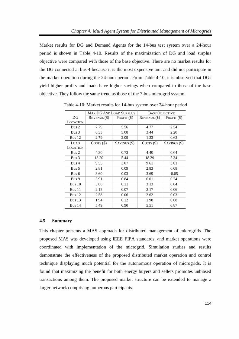
Chapter 4: Multi Agent System for Distributed Management of Microgrids
114
Market results for DG and Demand Agents for the 14-bus test system over a 24-hour
period is shown in Table 4-10. Results of the maximization of DG and load surplus
objective were compared with those of the base objective. There are no market results for
the DG connected at bus 4 because it is the most expensive unit and did not participate in
the market operation during the 24-hour period. From Table 4-10, it is observed that DGs
yield higher profits and loads have higher savings when compared to those of the base
objective. They follow the same trend as those of the 7-bus microgrid system.
Table 4-10: Market results for 14-bus system over 24-hour period
DG
LOCATION
MAX DG AND LOAD SURPLUS BASE OBJECTIVE REVENUE ($) PROFIT ($) REVENUE ($) PROFIT ($)
Bus 2 7.79 5.56 4.77 2.54 Bus 3 6.33 5.08 3.44 2.20
Bus 12 2.79 2.09 1.33 0.63 LOAD
LOCATION COSTS ($) SAVINGS ($) COSTS ($) SAVINGS ($)
Bus 2 4.30 0.73 4.40 0.64 Bus 3 18.20 5.44 18.29 5.34 Bus 4 9.55 3.07 9.61 3.01 Bus 5 2.81 0.09 2.83 0.08 Bus 6 3.60 0.03 3.69 -0.05 Bus 9 5.91 0.84 6.01 0.74
Bus 10 3.06 0.11 3.13 0.04 Bus 11 2.15 0.07 2.17 0.06 Bus 12 2.58 0.06 2.62 0.03 Bus 13 1.94 0.12 1.98 0.08 Bus 14 5.49 0.90 5.51 0.87
4.5 Summary
This chapter presents a MAS approach for distributed management of microgrids. The
proposed MAS was developed using IEEE FIPA standards, and market operations were
coordinated with implementation of the microgrid. Simulation studies and results
demonstrate the effectiveness of the proposed distributed market operation and control
technique displaying much potential for the autonomous operation of microgrids. It is
found that maximizing the benefit for both energy buyers and sellers promotes unbiased
transactions among them. The proposed market structure can be extended to manage a
larger network comprising numerous participants.
Chapter 4: Multi Agent System for Distributed Management of Microgrids
115
Furthermore, the proposed approach can be implemented in actual microgrids with
minimal additional software cost by replacing the Simulink models with the actual
microgrid and the communication network interface between MACSimJX and actual
microgrids can be achieved through TCP/IP and the necessary SCADA I/O devices.
Simulation studies have shown that the proposed distributed system is capable of handling
the economical and technical requirements of microgrids.
In terms of hardware implementation costs, it should be noted that there are some
differences between distributed and centralized operation. This comparison can be viewed
in terms of the interfacing and communication infrastructure costs. For the proposed MAS
approach, the associated hardware implementation costs which include the purchase of
modbus to TCP/IP converters/switches, the setup of the Internet and its associated
subscription costs are estimated to cost about US$5,000 based on the 7-bus microgrid
system. For centralized operation, the associated hardware implementation costs which
include the leasing of dedicated communication links as well as the installation of
communication wires for direct communication between these communication devices and
SCADA are estimated to cost about US$10,000 based on the 7-bus microgrid system. Note
that the cost of leasing dedicated communication links would be much higher than the
Internet subscription cost. Some price difference is expected between the different service
plans offered by different telcos. Therefore in comparison, an estimated saving of about
US$5,000 can be achieved by adopting the distributed MAS approach based on the 7-bus
microgrid system. Furthermore, this saving is scalable and more substantial in larger power
systems which may comprise thousands of DGs and load agents.
Chapter 5: Conclusion and Future Works
116
CHAPTER 5 CONCLUSION AND FUTURE WORKS
5.1 Conclusion
In this section, the significance, objectives and outcomes of this research are summarized.
This research discusses a distributed agent-based approach for the management of
microgrids and how this could contribute to the growing needs of modern restructured
power industry. It also explores the research of agent-based techniques in microgrids and
how the proposed approach can be extended to various aspects of power system operations
and the practical implications of adopting such an approach.
By utilizing agents to optimize the use of distributed power generation and load
consumption, the microgrid may be able to make a significant contribution by attempting
to reduce the energy prices and maximizing the welfare of every market participant. The
key objective is to maximize the benefits of energy sellers and energy buyers in an
unbiased manner. The distributed nature of agents provide great potential in the
management of numerous DGs and loads and allowing them to be adequately represented
and integrated into microgrids with minimal impact on the cost of communication
infrastructure. In this way, it is expected that the distributed approach can overcome the
limitations of centralized approach and can better handle microgrid operations when more
DGs are expected to integrate with the existing networks in future.
To understand the characteristics and behavioral properties of agent-based systems, the
concept of multi agent systems as well as the overall agent design and implementation are
introduced in Chapter 2. The IEEE FIPA specifications are used to standardize the design
and development of agents. JADE and MACSimJX have been identified as the most
suitable agent implementation software due to its compliance with FIPA standards as well
as their inherent advantage of shortening agent development time. The main objective is to
lay a Java-based agent framework for microgrid-based power market which would allow
an efficient distributed management of microgrids by maximizing the revenue of DGs
while minimizing the load costs. More specifically, the proposed market clearing algorithm
Chapter 5: Conclusion and Future Works
117
which considers incremental losses as part of its process and defines various agent
objectives is addressed in Chapter 4.
In Chapter 3, the design and development of customized agents for decentralized microgrid
operation was presented. Agent simulation was performed on JADE to test the
functionalities of the customized agents. These agents are programmed to consider the
market clearing price, agent's objective and electrical distance between each other as part
of the criteria to perform supply-demand matching and trading negotiations. Simulation
results have shown that MAS can effectively manage DGs as well as consider energy
prices for trading of energy within a microgrid.
In Chapter 4, a proposed microgrid market clearing technique and scheduling of DGs and
loads were presented. Two types of market bidding methods were discussed and a double-
side bidding which considers the submitted bids of DGs and loads was used in this thesis.
Subsequently, the MCP was determined from the intersection of the aggregated supply
curve and the aggregated demand curve. Next, the scheduling of each DG and load was
determined based on the MCP with respect to their respective individual supply/demand
curve. In addition, the LMP of each DG and load agent was considered. The loss
sensitivity factor, which is part of the marginal loss component in LMP was computed by
solving the inverse Jacobian matrix of the network using an IPM to obtain the phase angle
and voltage magnitudes and these values were subsequently used in the loss sensitivity
factor matrix. Furthermore, three different agent objectives were defined which basically
instruct agents to either maximize DG surplus or maximize load surplus or a combination
of both. The objectives of defining agent objectives is to analyze the effects of various
agent strategies on the proposed microgrid market clearing technique and to determine an
optimal strategy which benefits every market participant in the microgrid.
The proposed market structure was tested on a 7-bus microgrid power system in Chapter 4.
In market operations, DGs and price-sensitive loads participate in a microgrid energy
market implemented in JADE. Each DG and each price-sensitive load is represented by the
corresponding agents which perform various functions such as scheduling, coordination
and market clearing subject to system, DG and load constraints. Each agent is assigned to
Chapter 5: Conclusion and Future Works
118
one of the three agent objectives which maximizes either DG or load surpluses or both. In
the simulated operation of a microgrid, hourly power reference signals and load control
signals from JADE are passed on to DG and load models developed in
MATLAB/Simulink using MACSimJX. Simulated operation and dynamics of DGs and
loads are studied by performing simulations under different agent objectives. Simulation
results show that maximizing both the DG and load surplus objective provides optimal
benefits to both DGs and loads and is not biased to either side. Similar trends were also
observed for each hour during the study day. In addition, no voltage instability was
observed during the simulation. This shows that agents are able to handle the market
requirements as well as satisfy the power requirements of the microgrid under various
microgrid conditions.
To enhance the presentation of MCPs and marginal loss factor values, an extended
microgrid analysis on MCPs and marginal loss factor values to verify the effectiveness of
the proposed technique using a modified IEEE 14-bus test system is discussed in Chapter 4.
Simulation results show that the agents developed in this thesis are performing as intended
and are able to handle the market and power requirements of the microgrid. As expected,
the LMP values differ slightly from MCP due to the contribution from marginal loss
factors. Similarly, the maximization of DG and load surplus yields optimal benefits for
both the DGs and the loads compared to the other agent objectives. They follow the same
trend as those of the 7-bus microgrid power system. Therefore, it is found that maximizing
the benefit for both the energy buyers and energy sellers promotes unbiased transactions
between them. Simulation results of the IEEE 14-bus test system shows that the proposed
market structure can also be extended to manage a larger power network comprising
numerous participants.
5.2 Contribution of Thesis
Although many microgrid research activities involving MAS have been reported, no
proper MAS platform was implemented via integration of microgrid market operations and
DERs. The work reported in the literature specifically focuses on either intelligent market
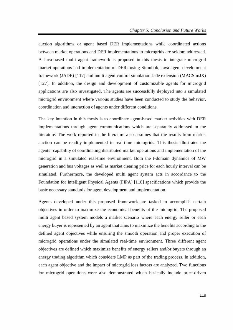
Chapter 5: Conclusion and Future Works
119
auction algorithms or agent based DER implementations while coordinated actions
between market operations and DER implementations in microgrids are seldom addressed.
A Java-based multi agent framework is proposed in this thesis to integrate microgrid
market operations and implementation of DERs using Simulink, Java agent development
framework (JADE) [117] and multi agent control simulation Jade extension (MACSimJX)
[127]. In addition, the design and development of customizable agents for microgrid
applications are also investigated. The agents are successfully deployed into a simulated
microgrid environment where various studies have been conducted to study the behavior,
coordination and interaction of agents under different conditions.
The key intention in this thesis is to coordinate agent-based market activities with DER
implementations through agent communications which are separately addressed in the
literature. The work reported in the literature also assumes that the results from market
auction can be readily implemented in real-time microgrids. This thesis illustrates the
agents’ capability of coordinating distributed market operations and implementation of the
microgrid in a simulated real-time environment. Both the t-domain dynamics of MW
generation and bus voltages as well as market clearing price for each hourly interval can be
simulated. Furthermore, the developed multi agent system acts in accordance to the
Foundation for Intelligent Physical Agents (FIPA) [118] specifications which provide the
basic necessary standards for agent development and implementation.
Agents developed under this proposed framework are tasked to accomplish certain
objectives in order to maximize the economical benefits of the microgrid. The proposed
multi agent based system models a market scenario where each energy seller or each
energy buyer is represented by an agent that aims to maximize the benefits according to the
defined agent objectives while ensuring the smooth operation and proper execution of
microgrid operations under the simulated real-time environment. Three different agent
objectives are defined which maximize benefits of energy sellers and/or buyers through an
energy trading algorithm which considers LMP as part of the trading process. In addition,
each agent objective and the impact of microgrid loss factors are analyzed. Two functions
for microgrid operations were also demonstrated which basically include price-driven
Chapter 5: Conclusion and Future Works
120
generation and demand scheduling and locational marginal pricing (LMP) [136, 143, 144]
for various participants in a distributed microgrid energy market.
5.3 Recommendation for Future Works
The following recommendations discuss future research and development works which
may provide additional insights into the application of MAS in the operation of microgrids.
In this thesis, the discussion and analysis of simulation results serve as a
preliminary step towards the design and hardware implementation of distributed
agent-based management for the efficient operation of microgrids. The proposed
MAS-based concept for distributed management of microgrids requires further
verification through the study and analysis of an actual experimental setup. A
125kW microgrid has been constructed at NTU under the A*STAR Intelligent
Energy Distribution System (IEDS) project initiatives and we plan to implement
the proposed MAS-based approach in the NTU microgrid.
There are also plans to study the application of MAS for the optimized operation of
interconnected electrical power supply networks as well as the chemical process
operations which load the networks under the Cambridge-NTU CREATE
Interdisciplinary Research Group (IRG) project which has begun in January 2014.
The main objective of this project is to reduce net energy consumption and/or
carbon and pollutant emissions for an integrated system of chemical plant loads and
the electrical supply network. Furthermore, it attempts to address issues arising
from evolving electrical systems having active load management, DG penetrations
at distribution level and demand response under unexpected peak demand
conditions. In addition, detailed studies will also be conducted on a Jurong Island
sub-network located in Singapore to address the growing demand and additional
power flows arising from centrally operated co-generation facilities.
Another future work is to extend the proposed MAS-based approach to ancillary
services [100, 145, 146] for microgrids. More specifically, the market structure
proposed in this thesis may be considered for frequency regulation in microgrids
Chapter 5: Conclusion and Future Works
121
[147, 148]. The objective of introducing frequency regulation markets in
microgrids is to further reduce the dependency on utility grid for power balancing.
Unlike traditional generators, the set points of power converter based DGs may be
pulsed faster than one second. This may be beneficial in stabilizing the frequency
in the microgrid. In addition, DGs may be able to further utilize any remaining
available capacity to competitively bid in frequency regulation markets after the
energy market has cleared. This can further maximize DG revenue and also help
improve the overall power quality of the microgrid. In this way, microgrids can be
more self-reliant and provide more economical benefits for the microgrid
participants.
The proposed MAS concept in this thesis considers the operation of a single
microgrid. However, there are also other operational issues which need to be
addressed when considering the coordination of multiple microgrids [97, 149].
Similar market mechanisms proposed in this thesis may be applied for multiple
microgrids but further studies are required to verify their effectiveness. By
considering the coordination of multiple microgrids, the research and development
of larger power systems such as smart grids will be reinforced.
In the simulation studies, the congestion component of the LMP was not considered
as no congestion is assumed in the illustrated system. However in practical systems,
the line capacity is considered to ensure that the power lines are not overload.
Therefore, sensitivity analysis using simulation software such as the PowerWorld
simulator could be done to include the congestion component in LMP and to
analyze its effects on the agent behaviors in the proposed market structure.
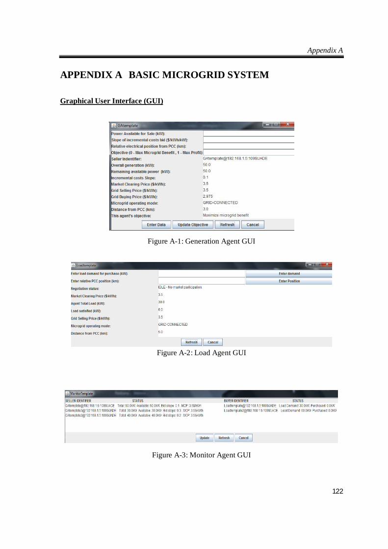
Appendix A
122
APPENDIX A BASIC MICROGRID SYSTEM
Graphical User Interface (GUI)
Figure A-1: Generation Agent GUI
Figure A-2: Load Agent GUI
Figure A-3: Monitor Agent GUI
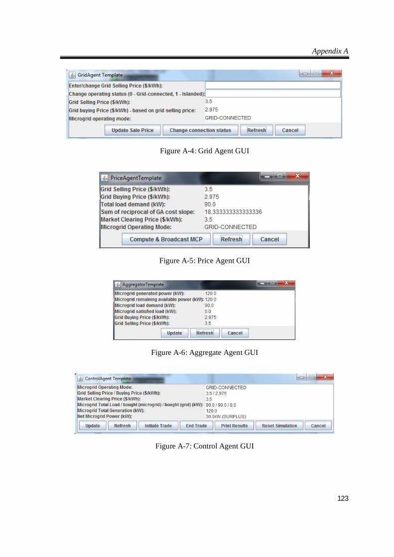
Appendix A
123
Figure A-4: Grid Agent GUI
Figure A-5: Price Agent GUI
Figure A-6: Aggregate Agent GUI
Figure A-7: Control Agent GUI
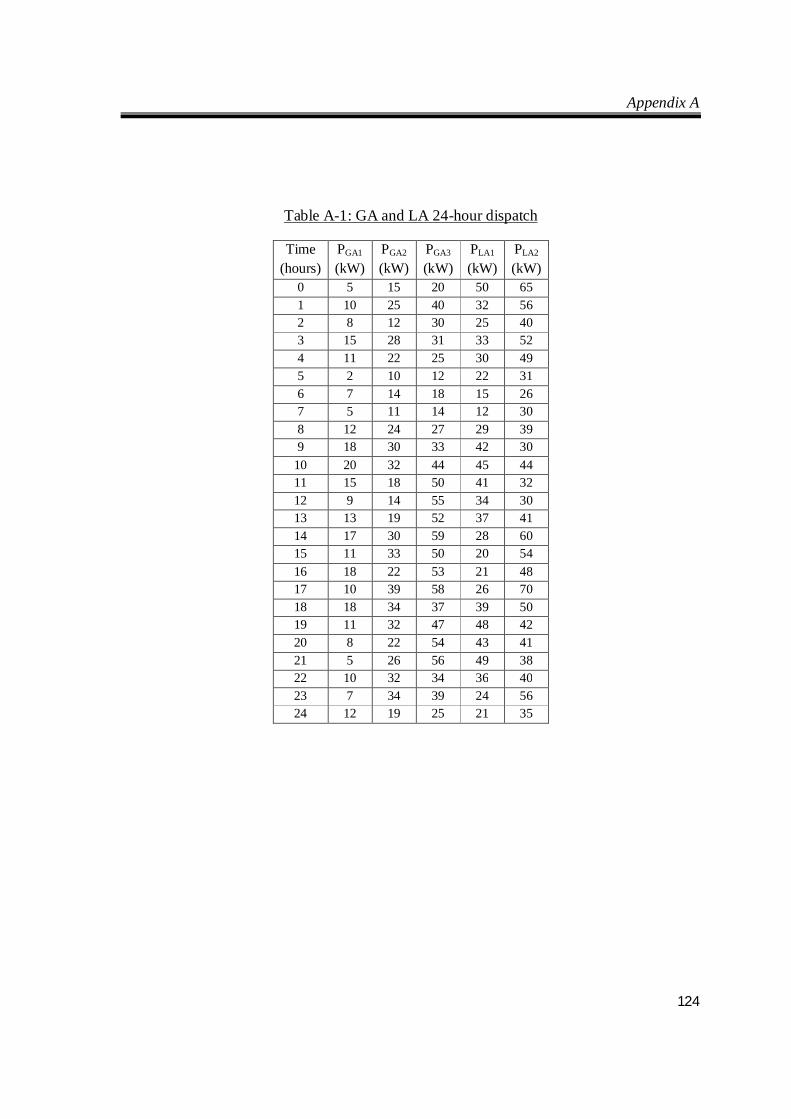
Appendix A
124
Table A-1: GA and LA 24-hour dispatch
Time (hours)
PGA1 (kW)
PGA2 (kW)
PGA3 (kW)
PLA1 (kW)
PLA2 (kW)
0 5 15 20 50 65 1 10 25 40 32 56 2 8 12 30 25 40 3 15 28 31 33 52 4 11 22 25 30 49 5 2 10 12 22 31 6 7 14 18 15 26 7 5 11 14 12 30 8 12 24 27 29 39 9 18 30 33 42 30
10 20 32 44 45 44 11 15 18 50 41 32 12 9 14 55 34 30 13 13 19 52 37 41 14 17 30 59 28 60 15 11 33 50 20 54 16 18 22 53 21 48 17 10 39 58 26 70 18 18 34 37 39 50 19 11 32 47 48 42 20 8 22 54 43 41 21 5 26 56 49 38 22 10 32 34 36 40 23 7 34 39 24 56 24 12 19 25 21 35
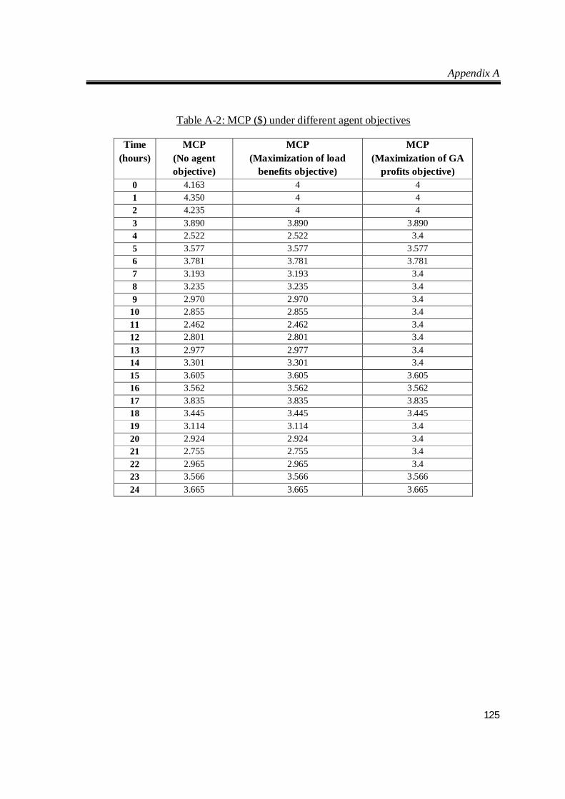
Appendix A
125
Table A-2: MCP ($) under different agent objectives
Time (hours)
MCP (No agent objective)
MCP (Maximization of load
benefits objective)
MCP (Maximization of GA
profits objective) 0 4.163 4 4 1 4.350 4 4 2 4.235 4 4 3 3.890 3.890 3.890 4 2.522 2.522 3.4 5 3.577 3.577 3.577 6 3.781 3.781 3.781 7 3.193 3.193 3.4 8 3.235 3.235 3.4 9 2.970 2.970 3.4
10 2.855 2.855 3.4 11 2.462 2.462 3.4 12 2.801 2.801 3.4 13 2.977 2.977 3.4 14 3.301 3.301 3.4 15 3.605 3.605 3.605 16 3.562 3.562 3.562 17 3.835 3.835 3.835 18 3.445 3.445 3.445 19 3.114 3.114 3.4 20 2.924 2.924 3.4 21 2.755 2.755 3.4 22 2.965 2.965 3.4 23 3.566 3.566 3.566 24 3.665 3.665 3.665
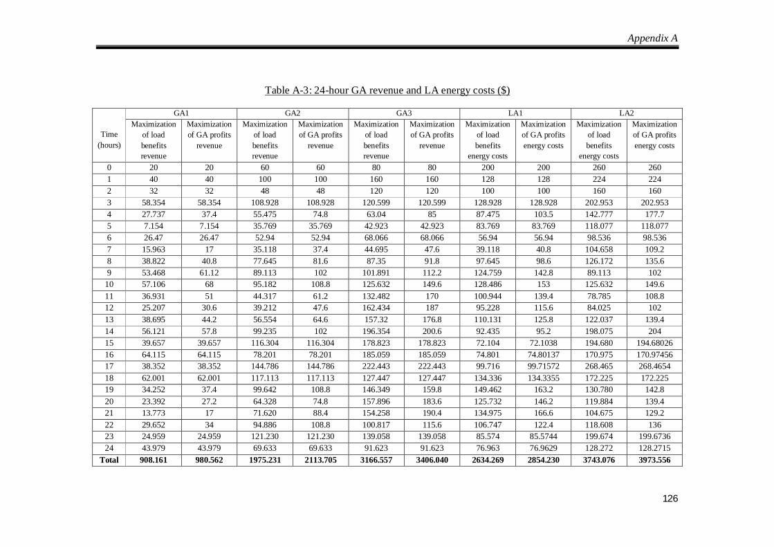
Appendix A
126
Table A-3: 24-hour GA revenue and LA energy costs ($)
Time (hours)
GA1 GA2 GA3 LA1 LA2 Maximization
of load benefits revenue
Maximization of GA profits
revenue
Maximization of load benefits revenue
Maximization of GA profits
revenue
Maximization of load benefits revenue
Maximization of GA profits
revenue
Maximization of load benefits
energy costs
Maximization of GA profits energy costs
Maximization of load benefits
energy costs
Maximization of GA profits energy costs
0 20 20 60 60 80 80 200 200 260 260 1 40 40 100 100 160 160 128 128 224 224 2 32 32 48 48 120 120 100 100 160 160 3 58.354 58.354 108.928 108.928 120.599 120.599 128.928 128.928 202.953 202.953 4 27.737 37.4 55.475 74.8 63.04 85 87.475 103.5 142.777 177.7 5 7.154 7.154 35.769 35.769 42.923 42.923 83.769 83.769 118.077 118.077 6 26.47 26.47 52.94 52.94 68.066 68.066 56.94 56.94 98.536 98.536 7 15.963 17 35.118 37.4 44.695 47.6 39.118 40.8 104.658 109.2 8 38.822 40.8 77.645 81.6 87.35 91.8 97.645 98.6 126.172 135.6 9 53.468 61.12 89.113 102 101.891 112.2 124.759 142.8 89.113 102
10 57.106 68 95.182 108.8 125.632 149.6 128.486 153 125.632 149.6 11 36.931 51 44.317 61.2 132.482 170 100.944 139.4 78.785 108.8 12 25.207 30.6 39.212 47.6 162.434 187 95.228 115.6 84.025 102 13 38.695 44.2 56.554 64.6 157.32 176.8 110.131 125.8 122.037 139.4 14 56.121 57.8 99.235 102 196.354 200.6 92.435 95.2 198.075 204 15 39.657 39.657 116.304 116.304 178.823 178.823 72.104 72.1038 194.680 194.68026 16 64.115 64.115 78.201 78.201 185.059 185.059 74.801 74.80137 170.975 170.97456 17 38.352 38.352 144.786 144.786 222.443 222.443 99.716 99.71572 268.465 268.4654 18 62.001 62.001 117.113 117.113 127.447 127.447 134.336 134.3355 172.225 172.225 19 34.252 37.4 99.642 108.8 146.349 159.8 149.462 163.2 130.780 142.8 20 23.392 27.2 64.328 74.8 157.896 183.6 125.732 146.2 119.884 139.4 21 13.773 17 71.620 88.4 154.258 190.4 134.975 166.6 104.675 129.2 22 29.652 34 94.886 108.8 100.817 115.6 106.747 122.4 118.608 136 23 24.959 24.959 121.230 121.230 139.058 139.058 85.574 85.5744 199.674 199.6736 24 43.979 43.979 69.633 69.633 91.623 91.623 76.963 76.9629 128.272 128.2715
Total 908.161 980.562 1975.231 2113.705 3166.557 3406.040 2634.269 2854.230 3743.076 3973.556
Appendix B
127
APPENDIX B INTERIOR POINT METHOD A nonlinear problem can be compactly described [150] which is given as:
min max
( )( ) 0
( )
Min f xsubject to g x
h h x h
(A.1)
where f(x) is the objective function to be minimized; g(x) is a vector of equality constraints;
h(x) consists of a vector of inequality constraints containing reactive power constraints;
and hmin and hmax are the corresponding lower and upper limits for h(x).
To convert the inequality constraints into equality ones, slack variables are introduced as:
min
max
( ) 0 0( ) 0 0
L L
U U
h x s h sh x s h s
(A.2)
where sL and sU are the respective lower and upper slack variables.
Using the logarithmic barrier function, the Lagrangian function can be established as
shown:
min
max
, , , , , , ( ) ( ) ( )
( ) ln ln
T TL U L U L L
TU U i Li i Ui
L s s s f x g x h x s h
h x s h s s
(A.3)
where the following parameters are defined as:
min
max
: Vector of Lagrangian multipliers for ( ) 0;: Vector of Lagrangian multipliers for ( ) 0;: Vector of Lagrangian multipliers for ( ) 0; and
: Barrier parameter.
L L
U U
g xh x s hh x s h
Next, the Karush Kuhn Tucker (KKT) first-order necessary optimality condition of the
Lagrangian function in (A.3) is derived as:
Appendix B
128
min
max
1
1
( ) ( ) ( ) 0( ) 0( ) 0
( ) 0
0
0
L
U
L
U
x x x x L U
L
U
s L L
s U U
L f x g x h xL g xL h x s h
L h x s h
L S e
L S e
(A.4)
where SL and SU are diagonal matrices containing the elements sL and sU as the diagonal
elements respectively; and e is a vector where all the elements are 1. Furthermore, the last
two equations in (A.4) are converted into the following equations for ease of differentiating
the KKT first-order condition.
0
0L
U
s L L
s U U
L S e e
L S e e
(A.5)
where L and U are diagonal matrices with the diagonal elements of L and U
respectively. With an initial guess, the correction equations of the first-order condition
using Newton’s method are shown as:
0
2 2 2
0
0
0
0
0
( ) ( )
( ) ( ) ( )
( )
( )
( )L
U
L
U
x x L U x
x x L U x
Tx
Tx L
Tx U
L L L L
U U U U
H x g x h x L
H g x h x f x
g x x Lh x x s L
h x x s L
S s L
S s L
(A.6)
where the right-hand side notations are the residuals of the KKT first-order condition
derived in (A.4) and (A.5).
In order to reduce the size of the above set of correction equations, the following linear
system which can be derived from (A.6) is shown as:

Appendix B
129
1 1
0 00 1 0 1 0 1 1
0
( )( ) 0
( ) ( )
( ) L UL U
xxT
x
Tx U U L L x
s sx x x L L U U L U
RxH g xRg x
H H h x S S h x
R L h x S L S L S L S L
R L
(A.7)
The following steps outline the procedures that are widely used in IPM:
1) Initialize the primal and dual variables.
2) Calculate the complementary gap: T TC L L U UG s s . If the gap and residuals is
smaller than the given tolerance, output the optimal solution and stop the process.
3) Calculate the barrier parameter with 2
CGr
where r is the number of constraints
and (0,1] is the centering parameter.
4) Solve the correction vectors andx in (A.7). After which, the parameters
, , and L U L Us s can be obtained from (A.6).
5) Update the primal and dual variables and return to step 2.
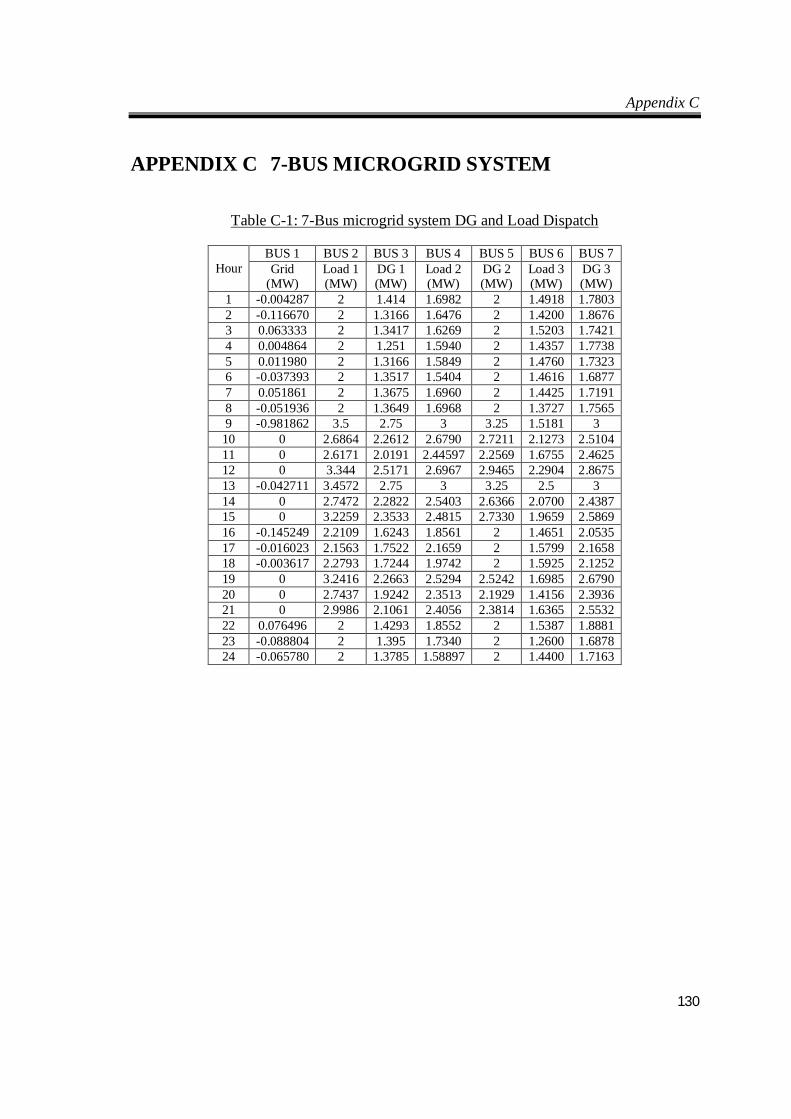
Appendix C
130
APPENDIX C 7-BUS MICROGRID SYSTEM
Table C-1: 7-Bus microgrid system DG and Load Dispatch
Hour
BUS 1 BUS 2 BUS 3 BUS 4 BUS 5 BUS 6 BUS 7 Grid
(MW) Load 1 (MW)
DG 1 (MW)
Load 2 (MW)
DG 2 (MW)
Load 3 (MW)
DG 3 (MW)
1 -0.004287 2 1.414 1.6982 2 1.4918 1.7803 2 -0.116670 2 1.3166 1.6476 2 1.4200 1.8676 3 0.063333 2 1.3417 1.6269 2 1.5203 1.7421 4 0.004864 2 1.251 1.5940 2 1.4357 1.7738 5 0.011980 2 1.3166 1.5849 2 1.4760 1.7323 6 -0.037393 2 1.3517 1.5404 2 1.4616 1.6877 7 0.051861 2 1.3675 1.6960 2 1.4425 1.7191 8 -0.051936 2 1.3649 1.6968 2 1.3727 1.7565 9 -0.981862 3.5 2.75 3 3.25 1.5181 3 10 0 2.6864 2.2612 2.6790 2.7211 2.1273 2.5104 11 0 2.6171 2.0191 2.44597 2.2569 1.6755 2.4625 12 0 3.344 2.5171 2.6967 2.9465 2.2904 2.8675 13 -0.042711 3.4572 2.75 3 3.25 2.5 3 14 0 2.7472 2.2822 2.5403 2.6366 2.0700 2.4387 15 0 3.2259 2.3533 2.4815 2.7330 1.9659 2.5869 16 -0.145249 2.2109 1.6243 1.8561 2 1.4651 2.0535 17 -0.016023 2.1563 1.7522 2.1659 2 1.5799 2.1658 18 -0.003617 2.2793 1.7244 1.9742 2 1.5925 2.1252 19 0 3.2416 2.2663 2.5294 2.5242 1.6985 2.6790 20 0 2.7437 1.9242 2.3513 2.1929 1.4156 2.3936 21 0 2.9986 2.1061 2.4056 2.3814 1.6365 2.5532 22 0.076496 2 1.4293 1.8552 2 1.5387 1.8881 23 -0.088804 2 1.395 1.7340 2 1.2600 1.6878 24 -0.065780 2 1.3785 1.58897 2 1.4400 1.7163
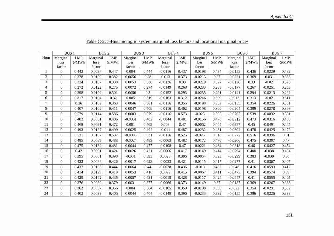
Appendix C
131
Table C-2: 7-Bus microgrid system marginal loss factors and locational marginal prices
Hour
BUS 1 BUS 2 BUS 3 BUS 4 BUS 5 BUS 6 BUS 7 Marginal
loss factor
LMP $/MWh
Marginal loss
factor
LMP $/MWh
Marginal loss
factor
LMP $/MWh
Marginal loss
factor
LMP $/MWh
Marginal loss
factor
LMP $/MWh
Marginal loss
factor
LMP $/MWh
Marginal loss
factor
LMP $/MWh
1 0 0.442 0.0097 0.447 0.004 0.444 -0.0116 0.437 -0.0198 0.434 -0.0155 0.436 -0.0229 0.432 2 0 0.378 0.0109 0.382 0.0056 0.38 -0.013 0.373 -0.0213 0.37 -0.0231 0.369 -0.031 0.366 3 0 0.334 0.0107 0.338 0.0053 0.336 -0.0136 0.33 -0.0219 0.327 -0.0128 0.33 -0.02 0.328 4 0 0.272 0.0122 0.275 0.0072 0.274 -0.0149 0.268 -0.0233 0.265 -0.0177 0.267 -0.0251 0.265 5 0 0.298 0.0109 0.301 0.0056 0.3 -0.0152 0.293 -0.0235 0.291 -0.0141 0.294 -0.0213 0.292 6 0 0.317 0.0104 0.32 0.005 0.319 -0.0163 0.312 -0.0246 0.309 -0.013 0.313 -0.02 0.311 7 0 0.36 0.0102 0.363 0.0046 0.361 -0.0116 0.355 -0.0198 0.352 -0.0155 0.354 -0.0226 0.351 8 0 0.407 0.0102 0.411 0.0047 0.409 -0.0116 0.402 -0.0198 0.399 -0.0204 0.399 -0.0278 0.396 9 0 0.579 0.0114 0.586 0.0003 0.579 -0.0116 0.573 -0.025 0.565 -0.0703 0.539 -0.0832 0.531 10 0 0.483 0.0061 0.486 -0.0031 0.482 -0.0044 0.481 -0.0156 0.476 -0.0212 0.473 -0.0316 0.468 11 0 0.468 0.0091 0.472 0.001 0.469 0.003 0.47 -0.0062 0.465 -0.0387 0.45 -0.0491 0.445 12 0 0.493 0.0127 0.499 0.0025 0.494 -0.011 0.487 -0.0232 0.481 -0.0304 0.478 -0.0425 0.472 13 0 0.531 0.0107 0.537 -0.0005 0.531 -0.0116 0.525 -0.025 0.518 -0.0272 0.516 -0.0396 0.51 14 0 0.485 0.0069 0.488 -0.0024 0.483 -0.0063 0.482 -0.0172 0.476 -0.0206 0.475 -0.0307 0.47 15 0 0.475 0.0139 0.481 0.0044 0.477 -0.0108 0.47 -0.0221 0.464 -0.0318 0.46 -0.0427 0.454 16 0 0.42 0.0091 0.424 0.0026 0.421 -0.0066 0.417 -0.0149 0.414 -0.0294 0.408 -0.038 0.404 17 0 0.395 0.0061 0.398 -0.001 0.395 0.0028 0.396 -0.0054 0.393 -0.0299 0.383 -0.039 0.38 18 0 0.422 0.0086 0.426 0.0017 0.423 -0.0033 0.421 -0.0115 0.417 -0.0277 0.41 -0.0367 0.407 19 0 0.437 0.0155 0.444 0.0064 0.44 -0.0028 0.436 -0.013 0.432 -0.048 0.416 -0.0593 0.412 20 0 0.414 0.0129 0.419 0.0053 0.416 0.0022 0.415 -0.0067 0.411 -0.0472 0.394 -0.0574 0.39 21 0 0.429 0.0142 0.435 0.0057 0.431 -0.0019 0.428 -0.0117 0.424 -0.0447 0.41 -0.0555 0.405 22 0 0.376 0.0089 0.379 0.0031 0.377 -0.0066 0.373 -0.0149 0.37 -0.0187 0.369 -0.0267 0.366 23 0 0.362 0.0097 0.366 0.004 0.364 -0.0105 0.359 -0.0188 0.356 -0.022 0.354 -0.0291 0.352 24 0 0.402 0.0099 0.406 0.0044 0.404 -0.0149 0.396 -0.0233 0.392 -0.0155 0.396 -0.0226 0.393
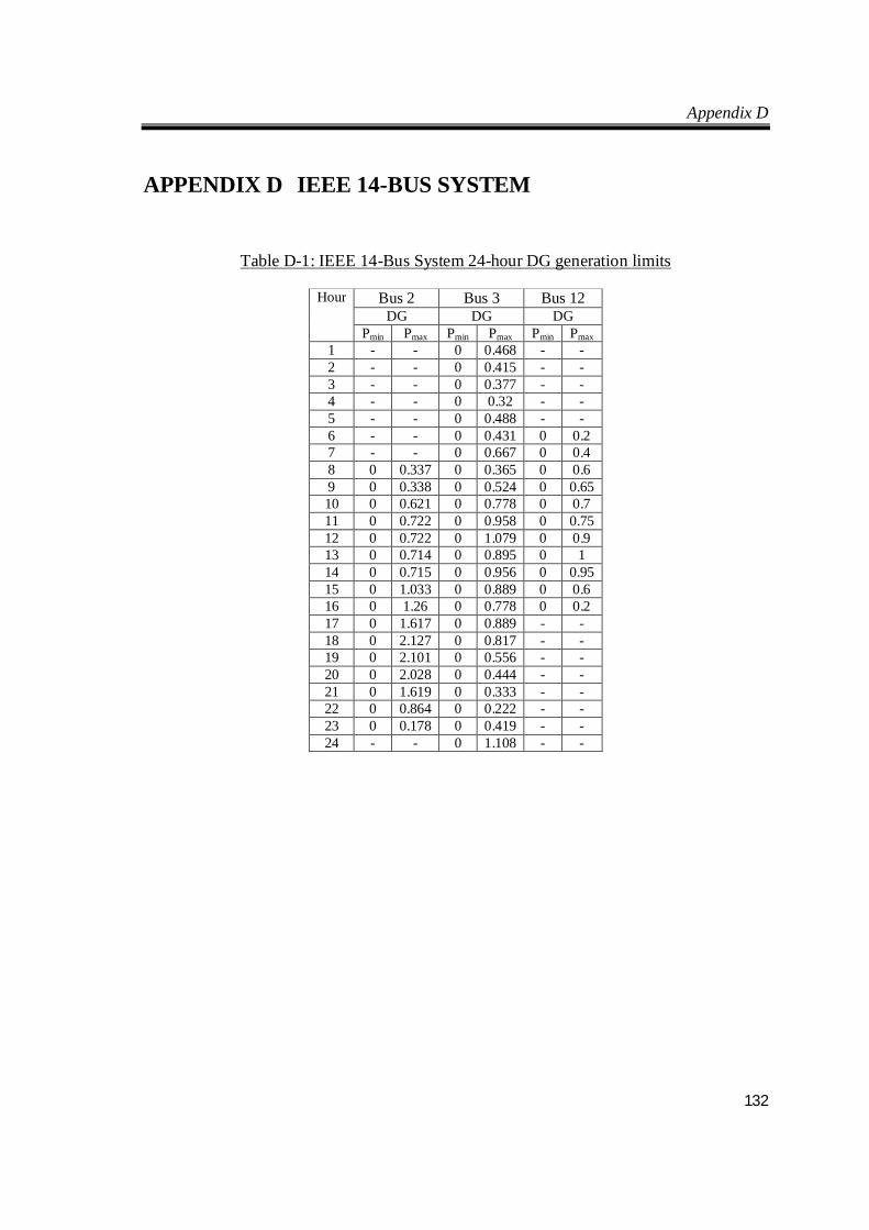
Appendix D
132
APPENDIX D IEEE 14-BUS SYSTEM
Table D-1: IEEE 14-Bus System 24-hour DG generation limits
Hour Bus 2 Bus 3 Bus 12 DG DG DG
Pmin Pmax Pmin Pmax Pmin Pmax 1 - - 0 0.468 - - 2 - - 0 0.415 - - 3 - - 0 0.377 - - 4 - - 0 0.32 - - 5 - - 0 0.488 - - 6 - - 0 0.431 0 0.2 7 - - 0 0.667 0 0.4 8 0 0.337 0 0.365 0 0.6 9 0 0.338 0 0.524 0 0.65 10 0 0.621 0 0.778 0 0.7 11 0 0.722 0 0.958 0 0.75 12 0 0.722 0 1.079 0 0.9 13 0 0.714 0 0.895 0 1 14 0 0.715 0 0.956 0 0.95 15 0 1.033 0 0.889 0 0.6 16 0 1.26 0 0.778 0 0.2 17 0 1.617 0 0.889 - - 18 0 2.127 0 0.817 - - 19 0 2.101 0 0.556 - - 20 0 2.028 0 0.444 - - 21 0 1.619 0 0.333 - - 22 0 0.864 0 0.222 - - 23 0 0.178 0 0.419 - - 24 - - 0 1.108 - -
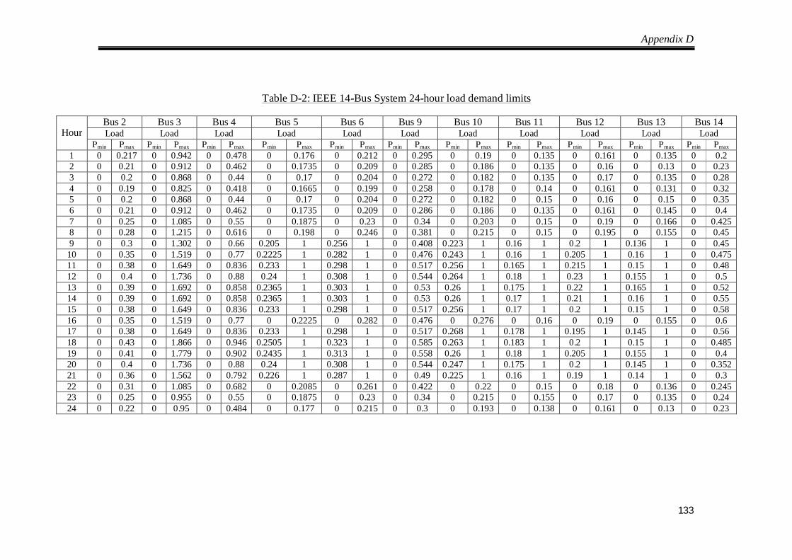
Appendix D
133
Table D-2: IEEE 14-Bus System 24-hour load demand limits
Hour
Bus 2 Bus 3 Bus 4 Bus 5 Bus 6 Bus 9 Bus 10 Bus 11 Bus 12 Bus 13 Bus 14 Load Load Load Load Load Load Load Load Load Load Load
Pmin Pmax Pmin Pmax Pmin Pmax Pmin Pmax Pmin Pmax Pmin Pmax Pmin Pmax Pmin Pmax Pmin Pmax Pmin Pmax Pmin Pmax 1 0 0.217 0 0.942 0 0.478 0 0.176 0 0.212 0 0.295 0 0.19 0 0.135 0 0.161 0 0.135 0 0.2 2 0 0.21 0 0.912 0 0.462 0 0.1735 0 0.209 0 0.285 0 0.186 0 0.135 0 0.16 0 0.13 0 0.23 3 0 0.2 0 0.868 0 0.44 0 0.17 0 0.204 0 0.272 0 0.182 0 0.135 0 0.17 0 0.135 0 0.28 4 0 0.19 0 0.825 0 0.418 0 0.1665 0 0.199 0 0.258 0 0.178 0 0.14 0 0.161 0 0.131 0 0.32 5 0 0.2 0 0.868 0 0.44 0 0.17 0 0.204 0 0.272 0 0.182 0 0.15 0 0.16 0 0.15 0 0.35 6 0 0.21 0 0.912 0 0.462 0 0.1735 0 0.209 0 0.286 0 0.186 0 0.135 0 0.161 0 0.145 0 0.4 7 0 0.25 0 1.085 0 0.55 0 0.1875 0 0.23 0 0.34 0 0.203 0 0.15 0 0.19 0 0.166 0 0.425 8 0 0.28 0 1.215 0 0.616 0 0.198 0 0.246 0 0.381 0 0.215 0 0.15 0 0.195 0 0.155 0 0.45 9 0 0.3 0 1.302 0 0.66 0.205 1 0.256 1 0 0.408 0.223 1 0.16 1 0.2 1 0.136 1 0 0.45 10 0 0.35 0 1.519 0 0.77 0.2225 1 0.282 1 0 0.476 0.243 1 0.16 1 0.205 1 0.16 1 0 0.475 11 0 0.38 0 1.649 0 0.836 0.233 1 0.298 1 0 0.517 0.256 1 0.165 1 0.215 1 0.15 1 0 0.48 12 0 0.4 0 1.736 0 0.88 0.24 1 0.308 1 0 0.544 0.264 1 0.18 1 0.23 1 0.155 1 0 0.5 13 0 0.39 0 1.692 0 0.858 0.2365 1 0.303 1 0 0.53 0.26 1 0.175 1 0.22 1 0.165 1 0 0.52 14 0 0.39 0 1.692 0 0.858 0.2365 1 0.303 1 0 0.53 0.26 1 0.17 1 0.21 1 0.16 1 0 0.55 15 0 0.38 0 1.649 0 0.836 0.233 1 0.298 1 0 0.517 0.256 1 0.17 1 0.2 1 0.15 1 0 0.58 16 0 0.35 0 1.519 0 0.77 0 0.2225 0 0.282 0 0.476 0 0.276 0 0.16 0 0.19 0 0.155 0 0.6 17 0 0.38 0 1.649 0 0.836 0.233 1 0.298 1 0 0.517 0.268 1 0.178 1 0.195 1 0.145 1 0 0.56 18 0 0.43 0 1.866 0 0.946 0.2505 1 0.323 1 0 0.585 0.263 1 0.183 1 0.2 1 0.15 1 0 0.485 19 0 0.41 0 1.779 0 0.902 0.2435 1 0.313 1 0 0.558 0.26 1 0.18 1 0.205 1 0.155 1 0 0.4 20 0 0.4 0 1.736 0 0.88 0.24 1 0.308 1 0 0.544 0.247 1 0.175 1 0.2 1 0.145 1 0 0.352 21 0 0.36 0 1.562 0 0.792 0.226 1 0.287 1 0 0.49 0.225 1 0.16 1 0.19 1 0.14 1 0 0.3 22 0 0.31 0 1.085 0 0.682 0 0.2085 0 0.261 0 0.422 0 0.22 0 0.15 0 0.18 0 0.136 0 0.245 23 0 0.25 0 0.955 0 0.55 0 0.1875 0 0.23 0 0.34 0 0.215 0 0.155 0 0.17 0 0.135 0 0.24 24 0 0.22 0 0.95 0 0.484 0 0.177 0 0.215 0 0.3 0 0.193 0 0.138 0 0.161 0 0.13 0 0.23

Appendix D
134
TABLE D-3: IEEE 14-BUS SYSTEM BIDDING RATES (mG, mD in $/MWh/MW) OVER 24-HOUR PERIOD
Hour Bus 2 Bus 3 Bus 4 Bus 5 Bus 6 Bus 9 Bus 10 Bus 11 Bus 12 Bus 13 Bus 14 DG Load DG Load Load Load Load Load Load Load DG Load Load Load
1 - 0.84 0.1 0.37 0.37 0.65 0.65 0.84 0.65 0.65 - 0.65 0.65 0.84 2 - 0.8 0.09 0.33 0.33 0.66 0.66 0.8 0.66 0.66 - 0.66 0.66 0.8 3 - 0.72 0.08 0.36 0.36 0.55 0.55 0.72 0.55 0.55 - 0.55 0.55 0.72 4 - 0.75 0.07 0.31 0.31 0.66 0.66 0.75 0.66 0.66 - 0.66 0.66 0.75 5 - 0.65 0.09 0.41 0.41 0.57 0.57 0.65 0.57 0.57 - 0.57 0.57 0.65 6 - 0.52 0.1 0.34 0.34 0.13 0.13 0.52 0.13 0.13 0.12 0.13 0.13 0.52 7 - 0.08 0.11 0.09 0.09 0.04 0.04 0.08 0.04 0.04 0.1 0.04 0.04 0.08 8 0.22 0.2 0.2 0.11 0.11 0.01 0.01 0.2 0.01 0.01 0.23 0.01 0.01 0.2 9 0.2 0.07 0.25 0.05 0.05 0.1 0.1 0.07 0.1 0.1 0.21 0.1 0.1 0.07 10 0.25 0.02 0.29 0.09 0.09 0.1 0.1 0.02 0.1 0.1 0.28 0.1 0.1 0.02 11 0.3 0.07 0.5 0.04 0.04 0.09 0.09 0.07 0.09 0.09 0.4 0.09 0.09 0.07 12 0.35 0.02 0.45 0.03 0.03 0.08 0.08 0.02 0.08 0.08 0.5 0.08 0.08 0.02 13 0.26 0.05 0.19 0.03 0.03 0.05 0.05 0.05 0.05 0.05 0.2 0.05 0.05 0.05 14 0.21 0.08 0.18 0.03 0.03 0.06 0.06 0.08 0.06 0.06 0.19 0.06 0.06 0.08 15 0.2 0.1 0.17 0.04 0.04 0.03 0.03 0.1 0.03 0.03 0.18 0.03 0.03 0.1 16 0.26 0.14 0.23 0.12 0.12 0.01 0.01 0.14 0.01 0.01 0.2 0.01 0.01 0.14 17 0.19 0.07 0.22 0.04 0.04 0.09 0.09 0.07 0.09 0.09 - 0.09 0.09 0.07 18 0.24 0.03 0.2 0.03 0.03 0.14 0.14 0.03 0.14 0.14 - 0.14 0.14 0.03 19 0.19 0.09 0.17 0.04 0.04 0.1 0.1 0.09 0.1 0.1 - 0.1 0.1 0.09 20 0.1 0.08 0.15 0.04 0.04 0.05 0.05 0.08 0.05 0.05 - 0.05 0.05 0.08 21 0.09 0.113 0.1 0.04 0.04 0.105 0.105 0.113 0.105 0.105 - 0.105 0.105 0.113 22 0.06 0.16 0.08 0.04 0.04 0.146 0.146 0.16 0.146 0.146 - 0.146 0.146 0.16 23 0.05 0.195 0.06 0.05 0.05 0.189 0.189 0.195 0.189 0.189 - 0.189 0.189 0.195 24 - 0.4 0.07 0.25 0.25 0.35 0.35 0.4 0.35 0.35 - 0.35 0.35 0.4
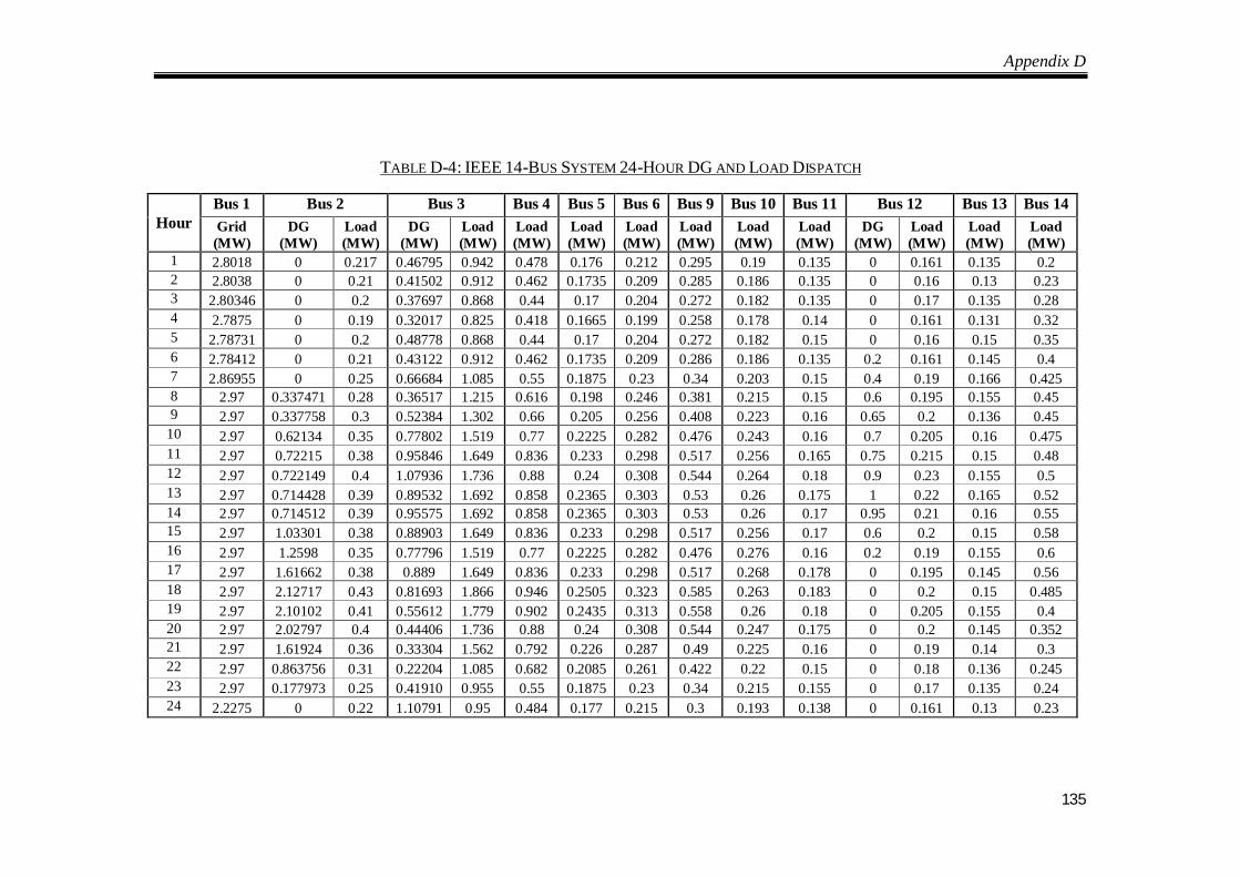
Appendix D
135
TABLE D-4: IEEE 14-BUS SYSTEM 24-HOUR DG AND LOAD DISPATCH
Hour
Bus 1 Bus 2 Bus 3 Bus 4 Bus 5 Bus 6 Bus 9 Bus 10 Bus 11 Bus 12 Bus 13 Bus 14 Grid (MW)
DG (MW)
Load (MW)
DG (MW)
Load (MW)
Load (MW)
Load (MW)
Load (MW)
Load (MW)
Load (MW)
Load (MW)
DG (MW)
Load (MW)
Load (MW)
Load (MW)
1 2.8018 0 0.217 0.46795 0.942 0.478 0.176 0.212 0.295 0.19 0.135 0 0.161 0.135 0.2 2 2.8038 0 0.21 0.41502 0.912 0.462 0.1735 0.209 0.285 0.186 0.135 0 0.16 0.13 0.23 3 2.80346 0 0.2 0.37697 0.868 0.44 0.17 0.204 0.272 0.182 0.135 0 0.17 0.135 0.28 4 2.7875 0 0.19 0.32017 0.825 0.418 0.1665 0.199 0.258 0.178 0.14 0 0.161 0.131 0.32 5 2.78731 0 0.2 0.48778 0.868 0.44 0.17 0.204 0.272 0.182 0.15 0 0.16 0.15 0.35 6 2.78412 0 0.21 0.43122 0.912 0.462 0.1735 0.209 0.286 0.186 0.135 0.2 0.161 0.145 0.4 7 2.86955 0 0.25 0.66684 1.085 0.55 0.1875 0.23 0.34 0.203 0.15 0.4 0.19 0.166 0.425 8 2.97 0.337471 0.28 0.36517 1.215 0.616 0.198 0.246 0.381 0.215 0.15 0.6 0.195 0.155 0.45 9 2.97 0.337758 0.3 0.52384 1.302 0.66 0.205 0.256 0.408 0.223 0.16 0.65 0.2 0.136 0.45
10 2.97 0.62134 0.35 0.77802 1.519 0.77 0.2225 0.282 0.476 0.243 0.16 0.7 0.205 0.16 0.475 11 2.97 0.72215 0.38 0.95846 1.649 0.836 0.233 0.298 0.517 0.256 0.165 0.75 0.215 0.15 0.48 12 2.97 0.722149 0.4 1.07936 1.736 0.88 0.24 0.308 0.544 0.264 0.18 0.9 0.23 0.155 0.5 13 2.97 0.714428 0.39 0.89532 1.692 0.858 0.2365 0.303 0.53 0.26 0.175 1 0.22 0.165 0.52 14 2.97 0.714512 0.39 0.95575 1.692 0.858 0.2365 0.303 0.53 0.26 0.17 0.95 0.21 0.16 0.55 15 2.97 1.03301 0.38 0.88903 1.649 0.836 0.233 0.298 0.517 0.256 0.17 0.6 0.2 0.15 0.58 16 2.97 1.2598 0.35 0.77796 1.519 0.77 0.2225 0.282 0.476 0.276 0.16 0.2 0.19 0.155 0.6 17 2.97 1.61662 0.38 0.889 1.649 0.836 0.233 0.298 0.517 0.268 0.178 0 0.195 0.145 0.56 18 2.97 2.12717 0.43 0.81693 1.866 0.946 0.2505 0.323 0.585 0.263 0.183 0 0.2 0.15 0.485 19 2.97 2.10102 0.41 0.55612 1.779 0.902 0.2435 0.313 0.558 0.26 0.18 0 0.205 0.155 0.4 20 2.97 2.02797 0.4 0.44406 1.736 0.88 0.24 0.308 0.544 0.247 0.175 0 0.2 0.145 0.352 21 2.97 1.61924 0.36 0.33304 1.562 0.792 0.226 0.287 0.49 0.225 0.16 0 0.19 0.14 0.3 22 2.97 0.863756 0.31 0.22204 1.085 0.682 0.2085 0.261 0.422 0.22 0.15 0 0.18 0.136 0.245 23 2.97 0.177973 0.25 0.41910 0.955 0.55 0.1875 0.23 0.34 0.215 0.155 0 0.17 0.135 0.24 24 2.2275 0 0.22 1.10791 0.95 0.484 0.177 0.215 0.3 0.193 0.138 0 0.161 0.13 0.23
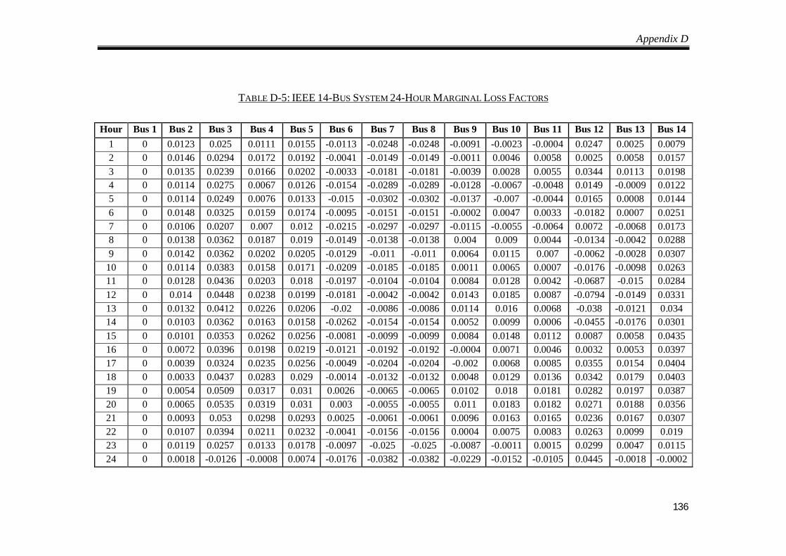
Appendix D
136
TABLE D-5: IEEE 14-BUS SYSTEM 24-HOUR MARGINAL LOSS FACTORS
Hour Bus 1 Bus 2 Bus 3 Bus 4 Bus 5 Bus 6 Bus 7 Bus 8 Bus 9 Bus 10 Bus 11 Bus 12 Bus 13 Bus 14 1 0 0.0123 0.025 0.0111 0.0155 -0.0113 -0.0248 -0.0248 -0.0091 -0.0023 -0.0004 0.0247 0.0025 0.0079 2 0 0.0146 0.0294 0.0172 0.0192 -0.0041 -0.0149 -0.0149 -0.0011 0.0046 0.0058 0.0025 0.0058 0.0157 3 0 0.0135 0.0239 0.0166 0.0202 -0.0033 -0.0181 -0.0181 -0.0039 0.0028 0.0055 0.0344 0.0113 0.0198 4 0 0.0114 0.0275 0.0067 0.0126 -0.0154 -0.0289 -0.0289 -0.0128 -0.0067 -0.0048 0.0149 -0.0009 0.0122 5 0 0.0114 0.0249 0.0076 0.0133 -0.015 -0.0302 -0.0302 -0.0137 -0.007 -0.0044 0.0165 0.0008 0.0144 6 0 0.0148 0.0325 0.0159 0.0174 -0.0095 -0.0151 -0.0151 -0.0002 0.0047 0.0033 -0.0182 0.0007 0.0251 7 0 0.0106 0.0207 0.007 0.012 -0.0215 -0.0297 -0.0297 -0.0115 -0.0055 -0.0064 0.0072 -0.0068 0.0173 8 0 0.0138 0.0362 0.0187 0.019 -0.0149 -0.0138 -0.0138 0.004 0.009 0.0044 -0.0134 -0.0042 0.0288 9 0 0.0142 0.0362 0.0202 0.0205 -0.0129 -0.011 -0.011 0.0064 0.0115 0.007 -0.0062 -0.0028 0.0307
10 0 0.0114 0.0383 0.0158 0.0171 -0.0209 -0.0185 -0.0185 0.0011 0.0065 0.0007 -0.0176 -0.0098 0.0263 11 0 0.0128 0.0436 0.0203 0.018 -0.0197 -0.0104 -0.0104 0.0084 0.0128 0.0042 -0.0687 -0.015 0.0284 12 0 0.014 0.0448 0.0238 0.0199 -0.0181 -0.0042 -0.0042 0.0143 0.0185 0.0087 -0.0794 -0.0149 0.0331 13 0 0.0132 0.0412 0.0226 0.0206 -0.02 -0.0086 -0.0086 0.0114 0.016 0.0068 -0.038 -0.0121 0.034 14 0 0.0103 0.0362 0.0163 0.0158 -0.0262 -0.0154 -0.0154 0.0052 0.0099 0.0006 -0.0455 -0.0176 0.0301 15 0 0.0101 0.0353 0.0262 0.0256 -0.0081 -0.0099 -0.0099 0.0084 0.0148 0.0112 0.0087 0.0058 0.0435 16 0 0.0072 0.0396 0.0198 0.0219 -0.0121 -0.0192 -0.0192 -0.0004 0.0071 0.0046 0.0032 0.0053 0.0397 17 0 0.0039 0.0324 0.0235 0.0256 -0.0049 -0.0204 -0.0204 -0.002 0.0068 0.0085 0.0355 0.0154 0.0404 18 0 0.0033 0.0437 0.0283 0.029 -0.0014 -0.0132 -0.0132 0.0048 0.0129 0.0136 0.0342 0.0179 0.0403 19 0 0.0054 0.0509 0.0317 0.031 0.0026 -0.0065 -0.0065 0.0102 0.018 0.0181 0.0282 0.0197 0.0387 20 0 0.0065 0.0535 0.0319 0.031 0.003 -0.0055 -0.0055 0.011 0.0183 0.0182 0.0271 0.0188 0.0356 21 0 0.0093 0.053 0.0298 0.0293 0.0025 -0.0061 -0.0061 0.0096 0.0163 0.0165 0.0236 0.0167 0.0307 22 0 0.0107 0.0394 0.0211 0.0232 -0.0041 -0.0156 -0.0156 0.0004 0.0075 0.0083 0.0263 0.0099 0.019 23 0 0.0119 0.0257 0.0133 0.0178 -0.0097 -0.025 -0.025 -0.0087 -0.0011 0.0015 0.0299 0.0047 0.0115 24 0 0.0018 -0.0126 -0.0008 0.0074 -0.0176 -0.0382 -0.0382 -0.0229 -0.0152 -0.0105 0.0445 -0.0018 -0.0002
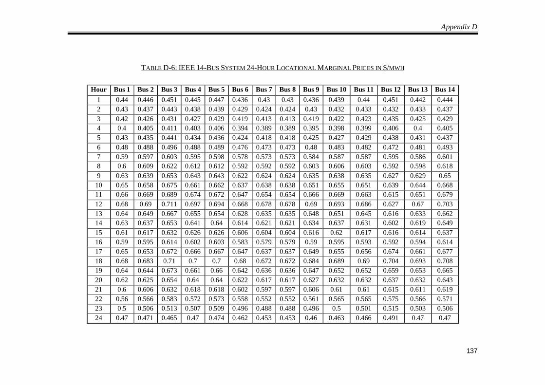
Appendix D
137
TABLE D-6: IEEE 14-BUS SYSTEM 24-HOUR LOCATIONAL MARGINAL PRICES IN $/MWH
Hour Bus 1 Bus 2 Bus 3 Bus 4 Bus 5 Bus 6 Bus 7 Bus 8 Bus 9 Bus 10 Bus 11 Bus 12 Bus 13 Bus 14 1 0.44 0.446 0.451 0.445 0.447 0.436 0.43 0.43 0.436 0.439 0.44 0.451 0.442 0.444 2 0.43 0.437 0.443 0.438 0.439 0.429 0.424 0.424 0.43 0.432 0.433 0.432 0.433 0.437 3 0.42 0.426 0.431 0.427 0.429 0.419 0.413 0.413 0.419 0.422 0.423 0.435 0.425 0.429 4 0.4 0.405 0.411 0.403 0.406 0.394 0.389 0.389 0.395 0.398 0.399 0.406 0.4 0.405 5 0.43 0.435 0.441 0.434 0.436 0.424 0.418 0.418 0.425 0.427 0.429 0.438 0.431 0.437 6 0.48 0.488 0.496 0.488 0.489 0.476 0.473 0.473 0.48 0.483 0.482 0.472 0.481 0.493 7 0.59 0.597 0.603 0.595 0.598 0.578 0.573 0.573 0.584 0.587 0.587 0.595 0.586 0.601 8 0.6 0.609 0.622 0.612 0.612 0.592 0.592 0.592 0.603 0.606 0.603 0.592 0.598 0.618 9 0.63 0.639 0.653 0.643 0.643 0.622 0.624 0.624 0.635 0.638 0.635 0.627 0.629 0.65
10 0.65 0.658 0.675 0.661 0.662 0.637 0.638 0.638 0.651 0.655 0.651 0.639 0.644 0.668 11 0.66 0.669 0.689 0.674 0.672 0.647 0.654 0.654 0.666 0.669 0.663 0.615 0.651 0.679 12 0.68 0.69 0.711 0.697 0.694 0.668 0.678 0.678 0.69 0.693 0.686 0.627 0.67 0.703 13 0.64 0.649 0.667 0.655 0.654 0.628 0.635 0.635 0.648 0.651 0.645 0.616 0.633 0.662 14 0.63 0.637 0.653 0.641 0.64 0.614 0.621 0.621 0.634 0.637 0.631 0.602 0.619 0.649 15 0.61 0.617 0.632 0.626 0.626 0.606 0.604 0.604 0.616 0.62 0.617 0.616 0.614 0.637 16 0.59 0.595 0.614 0.602 0.603 0.583 0.579 0.579 0.59 0.595 0.593 0.592 0.594 0.614 17 0.65 0.653 0.672 0.666 0.667 0.647 0.637 0.637 0.649 0.655 0.656 0.674 0.661 0.677 18 0.68 0.683 0.71 0.7 0.7 0.68 0.672 0.672 0.684 0.689 0.69 0.704 0.693 0.708 19 0.64 0.644 0.673 0.661 0.66 0.642 0.636 0.636 0.647 0.652 0.652 0.659 0.653 0.665 20 0.62 0.625 0.654 0.64 0.64 0.622 0.617 0.617 0.627 0.632 0.632 0.637 0.632 0.643 21 0.6 0.606 0.632 0.618 0.618 0.602 0.597 0.597 0.606 0.61 0.61 0.615 0.611 0.619 22 0.56 0.566 0.583 0.572 0.573 0.558 0.552 0.552 0.561 0.565 0.565 0.575 0.566 0.571 23 0.5 0.506 0.513 0.507 0.509 0.496 0.488 0.488 0.496 0.5 0.501 0.515 0.503 0.506 24 0.47 0.471 0.465 0.47 0.474 0.462 0.453 0.453 0.46 0.463 0.466 0.491 0.47 0.47
Author’s Vita
138
AUTHOR'S VITA Foo Yi Shyh Eddy was born in 1984 in Singapore. He received his Bachelor degree in
Electrical and Electronic Engineering (First Class Honours) from Nanyang Technological
University, Singapore, in 2009. His research interests include multi agent systems,
microgrids and electricity markets.
The author has the following publications.
Journal Publications
[1] Y. S. Foo. Eddy, H. B. Gooi and S. X. Chen, “Multi Agent System for Distributed
Management of Microgrids,” IEEE Transactions on Power Systems, vol.30, no.1,
pp.24,34, Jan. 2015.
[2] S. X. Chen, Y. S. Foo. Eddy, H. B. Gooi, M. Q. Wang and S. F. Lu, “A Centralized
Reactive Power Compensation System for LV Distribution Networks,” IEEE
Transactions on Power Systems, vol.30, no.1, pp.274,284, Jan. 2015.
[3] Nan Xia, H. B. Gooi, Ali Abur, S. X. Chen, Y. S. Foo. Eddy, “Enhanced State
Estimation Incorporating Adaptive Load Shedding Strategies as Pseudo
Measurements”, Under R1 revision review in IEEE Transactions on Power Systems,
2015.
Conference Publications
[1] Eddy, F. Y. S., Gooi, H. B., "Multi-Agent System for Optimization of
Microgrids," Power Electronics and ECCE Asia (ICPE & ECCE), 2011 IEEE 8th
International Conference on , vol., no., pp.2374,2381, Jeju, May 30 2011-June 3
2011.
[2] Tri Tran, Y. S. Foo. Eddy, K-V. Ling, “Application of Quadratically-Constrained
Model Predictive Control in Power Systems”, Accepted for publication in IEEE 13th
International Conference on Control, Automation, Robotics and Vision, Singapore,
December 10-12, 2014.
References
139
REFERENCES [1] A. Chambers, S. Hamilton, and B. Schnoor, Distributed Generation: A Nontechnical
Guide. Pennwell, 2001.
[2] L. Xuan and S. Bin, "Microgrids - an integration of renewable energy technologies,"
in Electricity Distribution, 2008. CICED 2008. China International Conference on,
2008, pp. 1-7.
[3] I. Wasiak, R. Pawelek, R. Mienski, and P. Gburczyk, "Using energy storage for
energy management and load compensation in LV microgrids," in Harmonics and
Quality of Power (ICHQP), 2012 IEEE 15th International Conference on, 2012, pp.
904-908.
[4] M. Triggianese, F. Liccardo, and P. Marino, "Ancillary Services performed by
Distributed Generation in grid integration," in Clean Electrical Power, 2007. ICCEP
'07. International Conference on, 2007, pp. 164-170.
[5] A. G. Tsikalakis and N. D. Hatziargyriou, "Centralized control for optimizing
microgrids operation," Energy Conv., IEEE Trans., vol. 23, pp. 241-248, 2008.
[6] P. Djapic, C. Ramsay, D. Pudjianto, G. Strbac, J. Mutale, N. Jenkins, and R. Allan,
"Taking an active approach," Power and Energy Magazine, IEEE, vol. 5, pp. 68-77,
2007.
[7] (2009). Distributed generation and Microgrid concept. Chapter 1. Available:
www.knovel.com
[8] R. C. Dugan and T. E. McDermott, "Operating conflicts for distributed generation on
distribution systems," in Proceedings in Rural Electric Power Conference, 2001, pp.
A3/1-A3/6.
[9] A. M. Azmy and I. Erlich, "Impact of distributed generation on the stability of
electrical power systems," in Proc. IEEE Power Engineering Society General
Meeting, 2005, pp. 1056-1063.
[10] Q. Sun, Z. Li, and H. Zhang, "Impact of distributed generation on voltage profile in
distribution system," in Proc. IEEE International Joint Conference on
Computational Sciences and Optimization, 2009, pp. 249-252.
References
140
[11] F. Bastiao, P. Cruz, and R. Fiteiro, "Impact of distributed generation on distribution
networks," in Proc. IEEE 5th International Conference on European Electricity
Market, 2008, pp. 1-6.
[12] R. A. Prata, "Impact of distributed generation connection with distribution grids -
two case-studies," in Proc. IEEE Power Engineering Society General Meeting, 2006,
pp. 1-8.
[13] P. P. Barker and R. W. D. Mello, "Determining the impact of distributed generation
on power systems: Part I – Radial distribution systems," in Proc. IEEE Power
Engineering Society Summer Meeting, 2000, pp. 1645-1656.
[14] A. P. S. Meliopoulos, "Distributed energy sources: Needs for analysis and design
tools," in Proc. IEEE Power Engineering Society Summer Meeting, 2001, pp. 548-
550.
[15] M. A. Lopez, S. Martin, J. A. Aguado, and S. de la Torre, "Market-oriented operation
in microGrids using multi-agent systems," in Power Eng., Energy and Electr. Drives
(POWERENG), 2011 Int. Conf., 2011, pp. 1-6.
[16] K. T. Tan, P. L. So, Y. C. Chu, and M. Z. Q. Chen, "Coordinated Control and Energy
Management of Distributed Generation Inverters in a Microgrid," Power Del., IEEE
Trans. on, vol. 28, pp. 704-713, 2013.
[17] F. Katiraei and M. R. Iravani, "Power management strategies for a microgrid with
multiple distributed generation units," IEEE Transactions on Power Delivery, vol. 21,
pp. 1821–1831, Nov. 2006.
[18] S. Chanana, "Some important aspects of price based frequency regulation and pricing
in competitive electricity markets," Department of Electrical Engineering, National
Institute of Technology Kurukshetra, Kurukshetra, India, April 2011.
[19] B. Lasseter, "Microgrids," in Proc. IEEE Power Engineering Society Winter Meeting,
2001, pp. 146-149.
[20] R. Lasseter, "Microgrids," in Proc. IEEE Power Engineering Society Winter Meeting,
2002, pp. 305-308.
[21] M. Barnes, J. Kondoh, H. Asano, J. Oyarzabal, G. Ventakaramanan, R. Lasseter, N.
Hatziargyriou, and T. Green, "Real-World MicroGrids-An Overview," in System of
References
141
Systems Engineering, 2007. SoSE '07. IEEE International Conference on, 2007, pp.
1-8.
[22] C. Shuaixun, "Modeling of lithium-ion battery for energy storage system
simulation," Master’s thesis, School of Electrical and Electronic Engineering,
Nanyang Technological University, 2008.
[23] G. Wand, Fuel cells history part 1. Tech. Rep.: Johnson Matthey, 2008.
[24] W. R. Grove, "On voltaic series and the combination of gases by platinum,"
Philosophical Magazine and Journal of Science, vol. XIV, pp. 127–130, Dec. 1838.
[25] W. R. Grove, "On a gaseous voltaic battery," Philosophical Magazine and Journal of
Science, vol. XXI, pp. 417–420, Mar. 1842.
[26] K. Nice and J. Strickland. How fuel cells work: Polymer exchange membrane fuel
cells [Online]. Available: http://auto.howstuffworks.com/fuel-efficiency/alternative-
fuels/fuel-cell2.htm
[27] N. Hatziargyriou, H. Asano, R. Iravani, and C. Marnay, "Microgrids," Power and
Energy Magazine, IEEE, vol. 5, pp. 78-94, 2007.
[28] R. H. Lasseter, A. Akhil, C. Marnay, J. Stephens, J. Dagle, R. Guttromson, A.
Meliopoulous, R. Yinger, and J. Eto, "The CERTS microgrid concept," White Paper
for Transmission Reliability Program Office of Power Technologies, U.S.
Department of Energy, 2002.
[29] M. Prodanovic and T. C. Green, "High-Quality Power Generation Through
Distributed Control of a Power Park Microgrid," Industrial Electronics, IEEE
Transactions on, vol. 53, pp. 1471-1482, 2006.
[30] F. Katiraei, R. Iravani, N. Hatziargyriou, and A. Dimeas, "Microgrids management,"
Power and Energy Magazine, IEEE, vol. 6, pp. 54-65, 2008.
[31] "IEEE standard for interconnecting distributed resources with electric power syst.,
IEEE Std. 1547," ed, 2003, reaffirmed 2008.
[32] F. Katiraei, M. R. Iravani, and P. W. Lehn, "Micro-grid autonomous operation during
and subsequent to islanding process," Power Delivery, IEEE Transactions on, vol. 20,
pp. 248-257, 2005.
References
142
[33] A. Mehrizi-Sani and R. Iravani, "Potential-Function Based Control of a Microgrid in
Islanded and Grid-Connected Modes," Power Systems, IEEE Transactions on, vol.
25, pp. 1883-1891, 2010.
[34] H. B. Gooi, P. L. So, E. K. Chan, E. Toh, and H. Gan, "Strait Ahead: Toward a
Sustainable, Economic, and Secure Electricity Supply in Singapore," Power and
Energy Magazine, IEEE, vol. 10, pp. 65-74, 2012.
[35] Microgrid Energy Management Systems [Online]. Available:
http://eeeweba.ntu.edu.sg/power_projects/mg-ems/default.asp
[36] R. Firestone and C. Marnay, "Energy manager design for microgrids," Consortium
for Electric Reliability Technology Solutions (CERTS), Tech. Rep.2005.
[37] R. Lasseter, A. Akhil, C. Marnay, J. Stephens, J. Dagle, R. Guttromson, A. P. S.
Meliopoulos, Y. Yinger, and P. Marino. Integration of Distributed Energy Resources
– The CERTS MicroGrid Concept [Online]. Available:
http://certs.lbl.gov/pdf/50829-app.pdf
[38] R. Lasseter, J. Eto, B. Schenkman, J. Stevens, H. Vollkommer, D. Klapp, E. Linton,
H. Hurtado, and J. Roy, "Certs microgrid laboratory test bed, and smart loads," IEEE
Transactions on Power Delivery, vol. 26, pp. 325–332, Jan. 2011.
[39] M. D. Ilić and S. X. Liu, "Hierarchical power systems control: Its value in a changing
industry (Advances in industrial control)," Springer, 1996.
[40] Aris Dimeas, Jose Oyarzabal, and N. Hatziargyriou. Demostration of MGCC in
laboratory with centralized and decentralized control [Online]. Available:
www.microgrids.eu/documents/642.pdf
[41] C. Marnay and G. Venkataramanan, "Microgrids in the evolving electricity
generation and delivery infrastructure," in Power Eng. Soc. Gen. Meet., 2006, IEEE,
2006, p. 5 pp.
[42] C. M. Colson and M. H. Nehrir, "A review of challenges to real-time power
management of microgrids," in Power & Energy Society General Meeting, 2009.
PES '09. IEEE, 2009, pp. 1-8.
[43] M. Ilic-Spong, J. Christensen, and K. L. Eichorn, "Secondary voltage control using
pilot point information," Power Syst., IEEE Trans., vol. 3, pp. 660-668, 1988.
References
143
[44] H. Chaoyong, H. Xuehao, and H. Dong, "Hierarchical control techniques applied in
micro-grid," in Power System Technology (POWERCON), 2010 International
Conference on, 2010, pp. 1-5.
[45] J. Zhenhua and R. A. Dougal, "Hierarchical microgrid paradigm for integration of
distributed energy resources," in Power and Energy Society General Meeting -
Conversion and Delivery of Electrical Energy in the 21st Century, 2008 IEEE, 2008,
pp. 1-8.
[46] T. L. Vandoorn, B. Zwaenepoel, J. D. M. De Kooning, B. Meersman, and L.
Vandevelde, "Smart microgrids and virtual power plants in a hierarchical control
structure," in Innovative Smart Grid Technologies (ISGT Europe), 2011 2nd IEEE
PES International Conference and Exhibition on, 2011, pp. 1-7.
[47] A. Bidram and A. Davoudi, "Hierarchical Structure of Microgrids Control System,"
Smart Grid, IEEE Transactions on, vol. 3, pp. 1963-1976, 2012.
[48] A.Afzalian and A. N. Niaki, "Hierarchical DES Supervisory Control Approach to
Microgrid Energy Systems," presented at the 21th International Power System
Conference, 2006.
[49] W. Caisheng, H. Nehrir, L. Feng, and Z. Junhui, "From hybrid energy systems to
microgrids: Hybridization techniques, configuration, and control," in Power and
Energy Society General Meeting, 2010 IEEE, 2010, pp. 1-4.
[50] J. M. Guerrero, J. C. Vasquez, J. Matas, L. G. de Vicuna, and M. Castilla,
"Hierarchical control of droop-controlled AC and DC microgrids - A general
approach toward standardization," Ind. Electron., IEEE Trans., vol. 58, pp. 158-172,
2011.
[51] Y. A. R. I. Mohamed and A. A. Radwan, "Hierarchical control system for robust
microgrid operation and seamless mode transfer in active distribution systems,"
Smart Grid, IEEE Trans., vol. 2, pp. 352-362, 2011.
[52] L. Phillipson and H. L. Willis, Understanding Electric Utilities and Deregulation.
New York: Marcell Decker Inc., 1999.
[53] S. Stoft, Power System Economics: Designing Markets for Electricity. NY: John
Wiley & Sons, 2002.
References
144
[54] D. Kirschen and G. Strbac, Fundamentals of Power System Economics. UK: John
Wiley and Sons, 2004.
[55] S. Hunt, Making Competition Work in Electricity. NY: John Wiley & Sons, 2002.
[56] K. Bhattacharya, M. H. J. Bollen, and J. E. Daalder, Operation of Restructured
Power Systems. Boston: Kluwer Academic Publishers, 2001.
[57] L. L. Lai, Power System Restructuring and Deregulation : Trading, Performance
and Information Technology. UK: John Wiley and Sons, 2001.
[58] M. Ilic, F. Galiana, and L. Fink, Power System Restructuring: Engineering and
Economics. Boston: Kluwer Academic Publishers, 1998.
[59] M. Shahidehpour, H. Yamin, and Z. Li, Market Operations in Electric Power System:
Forecasting Scheduling and Risk Management. NY: John Wiley & Sons, 2002.
[60] M. Shahidehpour and M. Alomoush, Restructured Electrical Power Systems,
Operation, Trading, and Volatility. New York: Marcel Dekker, Inc, 2001.
[61] Y.-H. Song and X.-F. Wang, Operation of Market-oriented Power Systems, . London:
Springer-Verlag, 2003.
[62] EMA. Singapore moving towards demand response and electricity futures trading
[Online]. Available: http://siew.sg/siew-news/singapore-moving-towards-demand-
response-and-electricity-futures-trading
[63] J. Zeng, J. Wu, J.-f. Liu, L.-m. Gao, and M. Li, "An agent-based approach to
renewable energy management in eco-building," in Sustainable Energy Technologies,
2008. ICSET 2008. IEEE International Conference on, 2008, pp. 46-50.
[64] J. Zhang, Q. Ai, C. Jiang, X. Wang, Z. Zheng, and C. Gu, "The application of multi
agent system in microgrid coordination control," in Sustainable Power Generation
and Supply, 2009. SUPERGEN '09. International Conference on, 2009, pp. 1-6.
[65] S. Suryanarayanan, J. Mitra, and S. Biswas, "A conceptual framework of a
hierarchically networked agent-based microgrid architecture," in Transmission and
Distribution Conference and Exposition, 2010 IEEE PES, 2010, pp. 1-5.
[66] M. K. Kouluri and R. K. Pandey, "Intelligent agent based micro grid control," in
Intelligent Agent and Multi-Agent Systems (IAMA), 2011 2nd Int. Conf., 2011, pp.
62-66.
References
145
[67] P. Dondi, D. Bayoumi, C. Haederli, D. Julian, and M. Suter, "Network integration of
distributed power generation," Journal of Power Sources, vol. 106, pp. 1-9, 2002.
[68] J. A. P. Lopes, N. Hatziargyriou, J. Mutale, P. Djapic, and N. Jenkins, "Integrating
distributed generation into electric power systems: A review of drivers, challenges
and opportunities," Electr. Power Syst. Res., vol. 77, pp. 1189-1203, 2007.
[69] K. De Brabandere, K. Vanthournout, J. Driesen, G. Deconinck, and R. Belmans,
"Control of microgrids," in Power Eng. Soc. Gen. Meet., 2007. IEEE, 2007, pp. 1-7.
[70] N. Hatziargyriou and A. P. S. Meliopoulos, "Distributed energy sources: technical
challenges," in Proc. IEEE Power Engineering Society Winter Meeting, 2002, pp.
1017-1022.
[71] P. Piagi and R. H. Lasseter, "Autonomous control of microgrids," in Power Eng. Soc.
Gen. Meet., 2006. IEEE, 2006, p. 8.
[72] T. Logenthiran, D. Srinivasan, and A. M. Khambadkone, "Multi-agent system for
energy resource scheduling of integrated microgrids in a distributed system," Electric
Power Systems Research, vol. 81, pp. 138-148, 2011.
[73] Z. Xiao, T. Li, M. Huang, J. Shi, J. Yang, J. Yu, and W. Wu. (2010, Hierarchical
MAS Based Control Strategy for Microgrid. 2, 1622-1638.
[74] A. L. Dimeas and N. D. Hatziargyriou, "Operation of a multiagent system for
microgrid control," IEEE Transactions on Power Systems, vol. 20, pp. 1447-1455,
2005.
[75] M. Pipattanasomporn, H. Feroze, and S. Rahman, "Multi-agent systems in a
distributed smart grid: Design and implementation," in Power Syst. Conf. and Expo.,
2009. PSCE '09. IEEE/PES, 2009, pp. 1-8.
[76] T. Logenthiran, D. Srinivasan, A. M. Khambadkone, and H. N. Aung, "Multi-Agent
System (MAS) for short-term generation scheduling of a microgrid," in Sustainable
Energy Technologies (ICSET), 2010 IEEE Int. Conf., 2010, pp. 1-6.
[77] T. Logenthiran, D. Srinivasan, A. M. Khambadkone, and A. Htay Nwe, "Multiagent
system for real-time operation of a microgrid in Real-Time Digital Simulator," Smart
Grid, IEEE Trans., vol. 3, pp. 925-933, 2012.
References
146
[78] P. H. Nguyen, W. L. Kling, and J. M. A. Myrzik, "Promising concepts and
technologies for future power delivery systems," in Universities Power Engineering
Conference, 2007. UPEC 2007. 42nd International, 2007, pp. 47-52.
[79] J. Oyarzabal, J. Jimeno, J. Ruela, A. Engler, and C. Hardt, "Agent based micro grid
management system," in Future Power Syst., 2005 Int. Conf., 2005, p. 6.
[80] X. Qun, J. Xiaobo, and H. Liqin, "The control of Distributed Generation System
using Multi-Agent System," in Electronics and Information Engineering (ICEIE),
2010 International Conference On, 2010, pp. V1-30-V1-33.
[81] M. S. Rajendram and R. K. Pandey, "Multi Agent Control for two area power system
network," in Computing, Electronics and Electrical Technologies (ICCEET), 2012
International Conference on, 2012, pp. 134-137.
[82] R. S. Salgado, C. F. Moyano, and A. D. R. Medeiros, "Reviewing strategies for
active power transmission loss allocation in power pools," International Journal of
Electrical Power & Energy Systems, vol. 26, pp. 81-90, 2004.
[83] L. M. Tolbert, Q. Hairong, and F. Z. Peng, "Scalable multi-agent system for real-
time electric power management," in Power Engineering Society Summer Meeting,
2001. IEEE, 2001, pp. 1676-1679 vol.3.
[84] Z. Wen-Di and C. Jin-Ding, "A multi-agent system for distributed energy resources
control in microgrid," in Critical Infrastructure (CRIS), 2010 5th International
Conference on, 2010, pp. 1-5.
[85] I. Zabet and M. Montazeri, "Decentralized control and management systems for
power industry via multiagent systems technology," in Power Engineering and
Optimization Conference (PEOCO), 2010 4th International, 2010, pp. 549-556.
[86] T. Logenthiran, D. Srinivasan, and D. Wong, "Multi-agent coordination for DER in
MicroGrid," in Sustainable Energy Technologies, 2008. ICSET 2008. IEEE
International Conference on, 2008, pp. 77-82.
[87] A. Dimeas and N. Hatziargyriou, "A multiagent system for microgrids," in Power
Engineering Society General Meeting, 2004. IEEE, 2004, pp. 55-58 Vol.1.
[88] A. L. Dimeas and N. D. Hatziargyriou, "A MAS architecture for microgrids control,"
in Intelligent Systems Application to Power Systems, 2005. Proceedings of the 13th
International Conference on, 2005, p. 5 pp.
References
147
[89] E. Kaegi, R. Cherkaoui, and A. Germond, "Decentralized Unit Commitment and
Dispatch for the Distribution Systems using Intelligent Agents Approach," presented
at the 16th PSCC, Glasgow, Scotland, 2008.
[90] Y. Nan-Peng, L. Chen-Ching, and J. Price, "Evaluation of Market Rules Using a
Multi-Agent System Method," Power Systems, IEEE Transactions on, vol. 25, pp.
470-479, 2010.
[91] C. M. Colson, M. H. Nehrir, and R. W. Gunderson, "Multi-agent Microgrid Power
Management," in 18th IFAC World Congress, Milano (Italy), August 2011.
[92] S. D. J. McArthur, E. M. Davidson, V. M. Catterson, A. L. Dimeas, N. D.
Hatziargyriou, F. Ponci, and T. Funabashi, "Multi-agent systems for power
engineering applications part I: Concepts, approaches, and technical challenges,"
Power Syst., IEEE Trans., vol. 22, pp. 1743-1752, 2007.
[93] S. D. J. McArthur, E. M. Davidson, V. M. Catterson, A. L. Dimeas, N. D.
Hatziargyriou, F. Ponci, and T. Funabashi, "Multi-agent systems for power
engineering applications part II: Technologies, standards, and tools for building
multi-agent systems," Power Syst., IEEE Trans., vol. 22, pp. 1753-1759, 2007.
[94] C. R. Robinson, "Decentralised Data Fusion Using Agents," Ph.D, Department of
Electronics, The University of York, 2008.
[95] D. Chun-Xia, J. Shi-Jiu, J. Guo-Tao, and B. Zhi-Qian, "Multi-agent based control
framework for microgrids," in Power and Energy Eng. Conf., 2009. APPEEC 2009.
Asia-Pacific, 2009, pp. 1-4.
[96] B. Mert, U. Aradag, S. Uludag, and H. O. Unver, "An architecture for a microgrid-
based eco industrial park using a Multi-Agent System," in Power Engineering,
Energy and Electrical Drives (POWERENG), 2013 Fourth International Conference
on, 2013, pp. 1658-1664.
[97] H. S. V. S. Kumar Nunna and S. Doolla, "Multiagent-Based Distributed-Energy-
Resource Management for Intelligent Microgrids," Ind. Electron., IEEE Trans., vol.
60, pp. 1678-1687, 2013.
[98] B. Ramachandran, S. K. Srivastava, C. S. Edrington, and D. A. Cartes, "An
Intelligent Auction Scheme for Smart Grid Market Using a Hybrid Immune
Algorithm," Ind. Electron., IEEE Trans. on, vol. 58, pp. 4603-4612, 2011.
References
148
[99] K. Hak-Man and T. Kinoshita, "Multiagent system for Microgrid operation based on
power market environment," in Telecommunications Energy Conference, 2009.
INTELEC 2009. 31st International, 2009, pp. 1-5.
[100] C. Yuen, A. Oudalov, and A. Timbus, "The Provision of Frequency Control Reserves
From Multiple Microgrids," Ind. Electron., IEEE Trans. on, vol. 58, pp. 173-183,
2011.
[101] D. P. Bertsekas and D. A. Castanon, "A forward/reverse auction algorithm for
asymmetric assignment problems," Comput. Optim. Appl., vol. 1, pp. 277-297, Dec.
1992.
[102] H. Feroze, "Multi-Agent Systems in Microgrids: Design and implementation,"
Virginia Polytechnic Institute and State University, Arlington, Virginia, Master of
Science thesis, 2009.
[103] F. Y. S. Eddy and H. B. Gooi, "Multi-agent system for optimization of microgrids,"
in Power Electronics and ECCE Asia (ICPE & ECCE), 2011 IEEE 8th International
Conference on, 2011, pp. 2374-2381.
[104] S. Russell and P. Norvig, Artificial intelligence: A modern approach, 2nd ed.: Upper
Saddle River, NJ: Prentice Hall, 2003.
[105] P. R. Cohen and H. J. Levesque, "Intention is choice with commitment. ," Artificial
Intelligence, vol. 42:213-261, 1990a.
[106] M. Wooldridge and N. R. Jennings, "Intelligent Agents: Theory and Practice," in
Knowledge Engineering Review 10(2), ed, 1995.
[107] J. Hintikka, "Knowledge and Belief," Cornell University Press: Ithaca, NY, 1962.
[108] A. S. Rao and M. P. Georgeff, "Asymmetry thesis and side-effect problems in linear
time and branching time intention logics," presented at the Proceedings of 12th
Internation Joint Conference on Artificial Intelligence, Sydney, Australia, 1991.
[109] R. Moore, A formal theory of knowledge and action: Morgan Kaufman, 1985.
[110] M. Wooldridge, "The logical modelling of computational multi-agent systems,"
Department of Computation, UMIST, 1992.
[111] M. Wooldridge and M. Fisher, "A first order branching-time logic of multi-agent
systems," in Proceedings of the 10th European Conference on Artifical Intelligence,
Vienna, Austria, 1992, pp. 234–238.
References
149
[112] E. Werner, "A unified view of information, intention and ability," in Proceedings of
the 2nd European Workshop on Modelling Autonomous Agents and Multi-Agent
Worlds, 1991, pp. 109–126.
[113] M. Singh, Multiagent Systems:A Theoretical Framework for Intentions vol. 799.
LNAI: Springer-Verlag, 1994.
[114] I. A. Ferguson, "TouringMachines: An Architecture for Dynamic, Rational, Mobile
Agents," Cambridge, UK, 1992.
[115] M. Wooldridge, "Intelligent agents," in G. Weiss, ed: Multi-agent systems, The MIT
Press, April 1999, pp. 3-51.
[116] S. D. J. McArthur, E. M. Davidson, and V. M. Catterson, "Building multi-agent
systems for power engineering applications," in Power Engineering Society General
Meeting, 2006. IEEE, 2006, p. 7 pp.
[117] Java Agent Development Framework (JADE) [Online]. Available:
http://jade.tilab.com/
[118] FIPA, The Foundation for Intelligent Physical Agents standard [Online]. Available:
http:/www.fipa.org/
[119] Y. Labrou , T. Finin , and Y. Peng, "Agent communication languages: The current
landscape," IEEE Intelligent Systems and their Applications, vol. 14 (2), pp. 45-52,
March/April 1999.
[120] O. Shehory, "Software architecture attributes of multi agent systems," in First
International Workshop on agent-oriented software engineering, 2001, pp. 77-90.
[121] FIPA ACL message structure specification [Online]. Available:
http://www.fipa.org/specs/fipa00061/SC00061G.pdf
[122] J. M. Vidal. FIPA Performatives [Online]. Available:
http://jmvidal.cse.sc.edu/talks/agentcommunication/performatives.html
[123] JADE API - ACL Message [Online]. Available:
http://jade.cselt.it/doc/api/jade/lang/acl/ACLMessage.html
[124] F. Bellifemine, A. Poggi, and G. Rimassa, "Developing Multi-agent Systems with
JADE," ed. Italy, 2001.
[125] C. Mangina, "Review of Software Products for Multi-Agent Systems," A. I. U. Ltd,
Ed., ed, 2002.
References
150
[126] P. Mendham and T. Clarke, "Macsim: A Simulink Enabled Environment for Multi-
Agent System Simulation," presented at the Proceedings of the 16th IFAC World
Congress, Prague, Czech Republic, 2005.
[127] Charles R. Robinson, Peter Mendham, and T. Clarke, "MACSimJX: A tool for
enabling agent modelling with simulink using JADE," Journal of Physical Agents,
vol. 4 no.3, 2010.
[128] I. Maity and S. Rao, "Simulation and Pricing Mechanism Analysis of a Solar-
Powered Electrical Microgrid," Systems Journal, IEEE, vol. 4, pp. 275-284, 2010.
[129] S. Chowdhury, S. P. Chowdhury, and P. Crossley, Microgrids and active distribution
networks: The Institution of Engineering and Technology, 2009.
[130] A. Sinha, A. K. Basu, R. N. Lahiri, S. Chowdhury, S. P. Chowdhury, and P. A.
Crossley, "Setting of market clearing price (MCP) in microgrid power scenario," in
Power and Energy Society General Meeting - Conversion and Delivery of Electrical
Energy in the 21st Century, 2008 IEEE, 2008, pp. 1-8.
[131] T. K. Panigrahi, A. K. Basu, S. Chowdhury, S. P. Chowdhury, N. Chakraborty, A.
Sinha, and Y. H. Song, "Emerging power market in a microgrid scenario," in
Universities Power Engineering Conference, 2007. UPEC 2007. 42nd International,
2007, pp. 1079-1085.
[132] D. Thukaram and C. Vyjayanthi, "Relative electrical distance concept for evaluation
of network reactive power and loss contributions in a deregulated system,"
Generation, Transmission & Distribution, IET, vol. 3, pp. 1000-1019, 2009.
[133] K. Visakha, D. Thukaram, and L. Jenkins, "Transmission charges of power contracts
based on relative electrical distances in open access," Electric Power Systems
Research, vol. 70, pp. 153-161, 2004.
[134] G. Yesuratnam and D. Thukaram, "Congestion management in open access based on
relative electrical distances using voltage stability criteria," Electric Power Systems
Research, vol. 77, pp. 1608-1618, 2007.
[135] S. Wong, K. Bhattacharya, and J. D. Fuller, "Coordination of Investor-Owned DG
Capacity Growth in Distribution Systems," Power Systems, IEEE Transactions on,
vol. 25, pp. 1375-1383, 2010.
References
151
[136] D. Gautam and N. Mithulananthan, "Optimal DG placement in deregulated
electricity market," Electric Power Systems Research, vol. 77, pp. 1627-1636, 2007.
[137] PowerWorld Simulator [Online]. Available: http://www.powerworld.com/
[138]A. J. Wood and B. F. Wollenberg, Power generation operation & control: New York:
John Wiley & Sons, 1984.
[139] S. X. Chen and H. B. Gooi, "Jump and shift method for multi-objective
optimization," Ind. Electron., IEEE Trans., vol. 58, pp. 4538-4548, 2011.
[140] K. T. Tan, P. L. So, and Y. C. Chu, "Control of parallel inverter-interfaced
distributed generation systems in microgrid for islanded operation," in Probabilistic
Methods Applied to Power Systems (PMAPS), 2010 IEEE 11th International
Conference on, 2010, pp. 1-5.
[141] Singapore electricity price information [Online]. Available:
http://www.emcsg.com/marketdata/priceinformation
[142] W. Hua, H. Sasaki, J. Kubokawa, and R. Yokoyama, "An interior point nonlinear
programming for optimal power flow problems with a novel data structure," Power
Syst., IEEE Trans on, vol. 13, pp. 870-877, 1998.
[143] R. Treinen, Locational Marginal Pricing (LMP): Basics of nodal price calculation
[Online]. Available:
http://www.caiso.com/docs/2004/02/13/200402131607358643.pdf
[144] D. Phillips. Nodal pricing basics [Online]. Available:
http://www.ieso.ca/imoweb/pubs/consult/mep/LMP_NodalBasics_2004jan14.pdf
[145] E. Ela, V. Gevorgian, A. Tuohy, B. Kirby, M. Milligan, and M. O'Malley, "Market
Designs for the Primary Frequency Response Ancillary Service - Part I: Motivation
and Design," Power Systems, IEEE Transactions on, vol. 29, pp. 421-431, 2014.
[146] E. Ela, V. Gevorgian, A. Tuohy, B. Kirby, M. Milligan, and M. O'Malley, "Market
Designs for the Primary Frequency Response Ancillary Service - Part II: Case
Studies," Power Systems, IEEE Transactions on, vol. 29, pp. 432-440, 2014.
[147] H. Bevrani, A. Ghosh, and G. Ledwich, "Renewable energy sources and frequency
regulation: survey and new perspectives," Renewable Power Generation, IET, vol. 4,
pp. 438-457, 2010.
References
152
[148] B. Biegel, L. H. Hansen, P. Andersen, and J. Stoustrup, "Primary Control by
ON/OFF Demand-Side Devices," Smart Grid, IEEE Transactions on, vol. 4, pp.
2061-2071, 2013.
[149] J. A. Aguado and V. H. Quintana, "Inter-utilities power-exchange coordination: a
market-oriented approach," Power Systems, IEEE Transactions on, vol. 16, pp. 513-
519, 2001.
[150] S. Hwachang, L. Byongjun, K. Sae-hyuk, and V. Ajjarapu, "Reactive reserve-based
contingency constrained optimal power flow (RCCOPF) for enhancement of voltage
stability margins," Power Systems, IEEE Transactions on, vol. 18, pp. 1538-1546,
2003.