A multigrid solver for 3D electromagnetic diffusion

Geophysical Prospecting, 2006, 54, 633–649

A multigrid solver for 3D electromagnetic diffusion

W.A. Mulder∗Shell International Exploration and Production, PO Box 60, 2280 AB Rijswijk, The Netherlands

Received March 2005, revision accepted March 2006

ABSTRACTThe performance of a multigrid solver for the time-harmonic electromagnetic problemin geophysical settings is investigated. The frequencies are sufficiently small for wavestravelling at the speed of light to be negligible, so that a diffusive problem remains.The discretization of the governing equations is obtained by the finite-integrationtechnique, which can be viewed as a finite-volume generalization of Yee’s staggeredgrid scheme. The resulting set of discrete equations is solved by a multigrid method.

The convergence rate of the multigrid method decreased when the grid wasstretched. The slower convergence rate of the multigrid method can be compensatedby using bicgstab2, a conjugate-gradient-type method for non-symmetric problems.In that case, the multigrid solver acts as a preconditioner. However, whereas the multi-grid method provides excellent convergence with constant grid spacings, it performsless than satisfactorily when substantial grid stretching is used.

I N T R O D U C T I O N

Numerical modelling of electromagnetic (EM) problems thatoccur in geophysics requires the solution of the Maxwell equa-tions in conducting media. For a particular class of prob-lems, waves that travel at the speed of light can be ignoredand diffusion dominates. This class includes magnetotelluricand controlled-source EM problems, but excludes ground-penetrating radar applications.

In two dimensions, the EM problem can be reduced to ascalar equation for either the out-of-plane electric or magneticfield. For an implicit time-step scheme or after transformationto the frequency domain, the spatial part of the operator isan elliptic equation. This Poisson-type equation with variablecoefficients can be solved efficiently by a direct method using,for instance, nested dissection (George and Liu 1981) or byan iterative method such as multigrid. The use of multigridmethods for elliptic problems has been well established sincethe 1980s. Solutions are typically obtained at a computationalcost that is about ten times the cost of evaluating the numericaldiscretization of the partial differential equations.

∗E-mail: [email protected]

In three dimensions, direct solvers incur such a high costthat they are not of practical use. Application of the multi-grid method is less straightforward than in 2D because of thelarge null-space of the curl-curl operator that occurs in theequations. A Helmholtz decomposition of the electric fieldinto potentials avoids that problem and produces a systemof Poisson-type equations (see e.g. Haber and Ascher 2001;Aruliah and Ascher 2003). The decomposition is unnecessarybecause in the late 1990s the problem of the null-space wassolved, either explicitly by taking care of the null-space com-ponents (Hiptmair 1998) or implicitly by solving small localsystems (Arnold et al. 2000). The second approach is usedhere.

The discretization is obtained by the finite-integration tech-nique (FIT) (Weiland 1977; Clemens and Weiland 2001),which can be viewed as a finite-volume generalization of Yee’sscheme (Yee 1966) for tensor-product Cartesian grids withvariable grid spacings. The scheme is reviewed in the sectionentitled Discretization. The multigrid solver is described inthe section entitled Multigrid Solver. It is a special case of themethod presented by Feigh et al. (2003), but with a differentrestriction operator.

The multigrid method can be used alone or as a precondi-tioner for a Krylov subspace method. The latter case may be

C© 2006 Shell International Explorations and Production BV 633

634 W.A. Mulder

necessary if the multigrid scheme has difficulties in removingcertain types of error. Here, we study convergence both forthe multigrid method alone and for bicgstab2 (van der Vorst1992; Gutknecht 1993) preconditioned by multigrid.

A number of numerical tests are presented in the section en-titled Examples. We start with an artificial test problem basedon sines and cosines. Next, a current source is considered,both in a homogeneous formation and in an inhomogeneousformation. Particular attention is paid to the effect of gridstretching.

A discussion of the numerical experiments and the mainconclusions is given in the section entitled Discussion and Con-

clusions.

D I S C R E T I Z AT I O N

Maxwell’s equations in the presence of a current source Js are

∂tB(x, t) + ∇ × E(x, t) = 0,

∇ × H(x, t) − ∂tD(x, t) = Jc(x, t) + Js(x, t),(1)

where the conduction current Jc obeys Ohm’s law,

Jc(x, t) = σ (x)E(x, t).

Here, σ (x) is the conductivity. E(x, t) is the electric fieldand H(x, t) is the magnetic field. The electric displacementD(x, t) = ε(x)E(x, t) and the magnetic induction B(x, t) =µ(x)H(x, t). The dielectric constant or permittivity ε can beexpressed as ε = ε rε0, where ε r is the relative permittivity andε0 is the vacuum value. Similarly, the magnetic permeability µ

can be written as µ = µr µ0, where µr is the relative perme-ability and µ0 is the vacuum value.

The magnetic field can be eliminated from (1), yielding thesecond-order parabolic system of equations,

ε∂ttE + σ∂tE + ∇ × µ−1∇ × E = −∂tJs.

To transform from the time domain to the frequency domain,we substitute

E(x, t) = 12π

∫ ∞

−∞E(x, ω)e−iωtdω,

and use a similar representation for H(x, t). The resulting sys-tem of equations is

iωµ0σ E − ∇ × µ−1r ∇ × E = −iωµ0Js, (2)

where σ (x) = σ − iωε. Here, only low frequencies are con-sidered that obey |ωε| � σ . From here on, the hats ˆ(.) areomitted. We use the perfectly electrically conducting boundary

conditions:

n × E = 0 and n · H = 0, (3)

where n is the outward normal on the boundary of the domain.Equation (2) can be discretized by the finite-integration

technique (Weiland 177; Clemens and Weiland 2001). Thisscheme can be viewed as a finite-volume generalization ofYee’s (1966) scheme for tensor-product Cartesian grids withvariable grid spacings. An error analysis for the constant-coefficient case (Monk and Suli 1994) showed that both theelectric and magnetic field components have second-orderaccuracy.

Consider a tensor-product Cartesian grid with nodes at po-sitions (xk, yl, zm), where k = 0, . . . , Nx, l = 0, . . . , Ny andm = 0, . . . , Nz. There are Nx × Ny × Nz cells having thesenodes as vertices. The cell centres are located at

xk+1/2 = 12 (xk + xk+1),

yl+1/2 = 12 (yl + yl+1),

zm+1/2 = 12 (zm + zm+1). (4)

(xk,yl+1,zm+1)

(xk,yl,zm+1)(xk+1,yl+1,zm+1)

(xk+1,yl+1,zm)

(xk+1,yl,zm)

(xk,yl,zm)

E3

E2E1

(xk+1,yl+1,zm+1)

(xk+1,yl+1,zm)

(xk+1,yl,zm)

H1

H2

(xk,yl,zm)

(xk,yl,zm+1)

(xk,yl+1,zm+1) H3

(a)

(b)

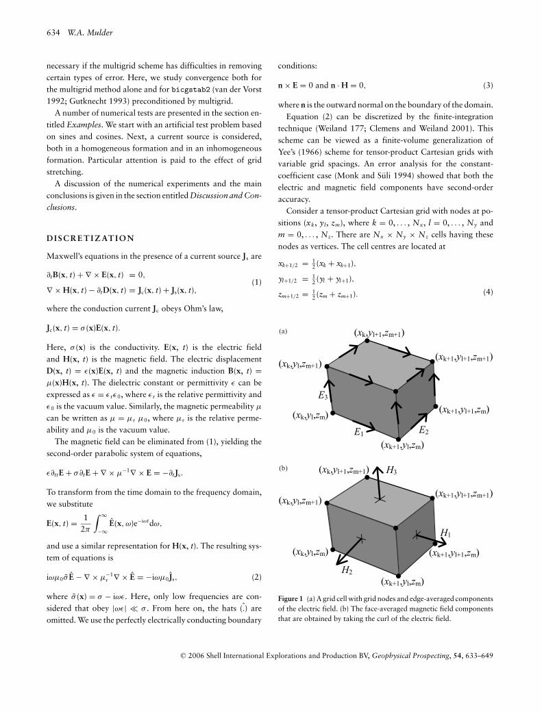
Figure 1 (a) A grid cell with grid nodes and edge-averaged componentsof the electric field. (b) The face-averaged magnetic field componentsthat are obtained by taking the curl of the electric field.

C© 2006 Shell International Explorations and Production BV, Geophysical Prospecting, 54, 633–649

Multigrid for 3D EM 635

The material properties, σ and µ−1r , are assumed to be given as

cell-averaged values. The electric field components are posi-tioned at the edges of the cells, as shown in Fig. 1, in a mannersimilar to Yee’s scheme. The first component of the electricfield E1,k+1/2,l,m should approximate the average of E1(x, yl,zm) over the edge from xk to xk+1 at given yl and zm. Here,the average is defined as the line integral divided by the lengthof the integration interval. The other components, E2,k,l+1/2,m

and E3,k,l,m+1/2, are defined in a similar way. Note that theseaverages may also be interpreted as point values at the mid-point of edges:

E1,k+1/2,l,m � E1(xk+1/2, yl , zm),

E2,k,l+1/2,m � E2(xk, yl+1/2, zm),

E3,k,l,m+1/2 � E3(xk, yl , zm+1/2).

The averages and point-values are the same within second-order accuracy.

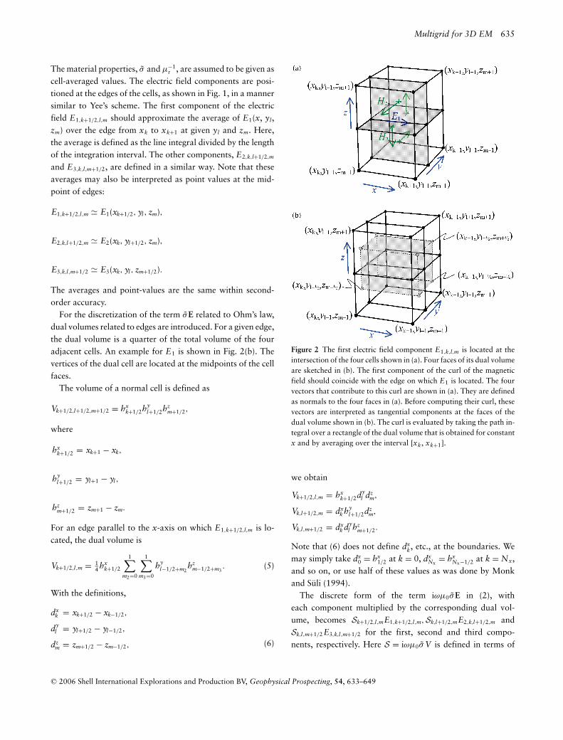
For the discretization of the term σE related to Ohm’s law,dual volumes related to edges are introduced. For a given edge,the dual volume is a quarter of the total volume of the fouradjacent cells. An example for E1 is shown in Fig. 2(b). Thevertices of the dual cell are located at the midpoints of the cellfaces.

The volume of a normal cell is defined as

Vk+1/2,l+1/2,m+1/2 = hxk+1/2hy

l+1/2hzm+1/2,

where

hxk+1/2 = xk+1 − xk,

hyl+1/2 = yl+1 − yl ,

hzm+1/2 = zm+1 − zm.

For an edge parallel to the x-axis on which E1,k+1/2,l,m is lo-cated, the dual volume is

Vk+1/2,l,m = 14 hx

k+1/2

1∑m2=0

1∑m3=0

hyl−1/2+m2

hzm−1/2+m3

. (5)

With the definitions,

dxk = xk+1/2 − xk−1/2,

dyl = yl+1/2 − yl−1/2,

dzm = zm+1/2 − zm−1/2, (6)

Figure 2 The first electric field component E1,k,l,m is located at theintersection of the four cells shown in (a). Four faces of its dual volumeare sketched in (b). The first component of the curl of the magneticfield should coincide with the edge on which E1 is located. The fourvectors that contribute to this curl are shown in (a). They are definedas normals to the four faces in (a). Before computing their curl, thesevectors are interpreted as tangential components at the faces of thedual volume shown in (b). The curl is evaluated by taking the path in-tegral over a rectangle of the dual volume that is obtained for constantx and by averaging over the interval [xk, xk+1].

we obtain

Vk+1/2,l,m = hxk+1/2dy

l dzm,

Vk,l+1/2,m = dxk hy

l+1/2dzm,

Vk,l,m+1/2 = dxk dy

l hzm+1/2.

Note that (6) does not define dxk, etc., at the boundaries. We

may simply take dx0 = hx

1/2 at k = 0, dxNx

= hxNx−1/2 at k = Nx,

and so on, or use half of these values as was done by Monkand Suli (1994).

The discrete form of the term iωµ0σE in (2), witheach component multiplied by the corresponding dual vol-ume, becomes Sk+1/2,l,mE1,k+1/2,l,m,Sk,l+1/2,mE2,k,l+1/2,m andSk,l,m+1/2 E3,k,l,m+1/2 for the first, second and third compo-nents, respectively. Here S = iωµ0σ V is defined in terms of


636 W.A. Mulder

cell-averages. At the edges parallel to the x-axis, an averagingprocedure similar to (5) gives

Sk+1/2,l,m = 14 (Sk+1/2,l−1/2,m−1/2 + Sk+1/2,l+1/2,m−1/2

+Sk+1/2,l−1/2,m+1/2 + Sk+1/2,l+1/2,m+1/2).

Sk,l+1/2,m and Sk,l,m+1/2 are defined in a similar way.The curl of E follows from path integrals around the edges

that bound a face of a cell, drawn in Fig. 1(a). After divisionby the area of the faces, the result is a face-averaged valuethat can be positioned at the centre of the face, as sketched inFig. 1(b). If this result is divided by iωµ, the component of themagnetic field that is normal to the face is obtained. In orderto find the curl of the magnetic field, the magnetic field com-ponents that are normal to faces are interpreted as tangentialcomponents at the faces of the dual volumes. For E1, this isshown in Fig. 2. For the first component of equation (2) onthe edge (k + 1

2 , l, m) connecting (xk, yl, zm) and (xk+1, yl, zm),the corresponding dual volume comprises the set [xk, xk+1] ×[yl−1/2, yl+1/2] × [zm−1/2, zm+1/2] having volume Vk+1/2,l,m.

The scaling by µ−1r at the face requires another averaging

step because the material properties are assumed to be givenas cell-averaged values. We define M = Vµ−1

r , so

Mk+1/2,l+1/2,m+1/2 = hxk+1/2hy

l+1/2hzm+1/2µ

−1r,k+1/2,l+1/2,m+1/2

for a given cell (k + 12 , l + 1

2 , m + 12 ). An averaging step in, for

instance, the z-direction gives

Mk+1/2,l+1/2,m = 12 (Mk+1/2,l+1/2,m−1/2 + Mk+1/2,l+1/2,m+1/2)

at the face (k + 12 , l + 1

2 , m) between the cells (k + 12 , l +

12 , m − 1

2 ) and (k + 12 , l + 1

2 , m + 12 ).

Starting with v = ∇ × E, we have

v1,k,l+1/2,m+1/2 = eyl+1/2(E3,k,l+1,m+1/2 − E3,k,l,m+1/2)

− ezm+1/2(E2,k,l+1/2,m+1 − E2,k,l+1/2,m),

v2,k+1/2,l,m+1/2 = ezm+1/2(E1,k+1/2,l,m+1 − E1,k+1/2,l,m)

− exk+1/2(E3,k+1,l,m+1/2 − E3,k,l,m+1/2),

v3,k+1/2,l+1/2,m = exk+1/2(E2,k+1,l+1/2,m − E2,k,l+1/2,m)

− eyl+1/2(E1,k+1/2,l+1,m − E1,k+1/2,l,m). (7)

Here,

exk+1/2 = 1/hx

k+1/2, eyl+1/2 = 1/hy

l+1/2, ezm+1/2 = 1/hz

m+1/2.

Next, we let

u1,k,l+1/2,m+1/2 = Mk,l+1/2,m+1/2v1,k,l+1/2,m+1/2,

u2,k+1/2,l,m+1/2 = Mk+1/2,l,m+1/2v2,k+1/2,l,m+1/2,

u3,k+1/2,l+1/2,m = Mk+1/2,l+1/2,mv3,k+1/2,l+1/2,m.

Note that these components are related to the magnetic fieldcomponents by

u1,k,l+1/2,m+1/2 = iωµ0Vk,l+1/2,m+1/2 H1,k,l+1/2,m+1/2,

u2,k+1/2,l,m+1/2 = iωµ0Vk+1/2,l,m+1/2 H2,k+1/2,l,m+1/2,

u3,k+1/2,l+1/2,m = iωµ0Vk+1/2,l+1/2,mH3,k+1/2,l+1/2,m,

where

Vk,l+1/2,m+1/2 = dxk hy

l+1/2hzm+1/2,

Vk+1/2,l,m+1/2 = hxk+1/2dy

l hzm+1/2,

Vk+1/2,l+1/2,m = hxk+1/2hy

l+1/2dzm.

The discrete representation of the source term i ωµ0 Js, mul-tiplied by the appropriate dual volume, is

s1,k+1/2,l,m = iωµ0Vk+1/2,l,mJ1,k+1/2,l,m,

s2,k,l+1/2,m = iωµ0Vk,l+1/2,mJ2,k,l+1/2,m,

s3,k,l,m+1/2 = iωµ0Vk,l,m+1/2 J3,k,l,m+1/2.

Let the residual for an arbitrary electric field that is not nec-essarily a solution to the problem be defined as

r = V(iωµ0Js + iωµ0σE − ∇ × µ−1

r ∇ × E).

Its discretization is

r1,k+1/2,l,m = s1,k+1/2,l,m + Sk+1/2,l,mE1,k+1/2,l,m

−[ey

l+1/2u3,k+1/2,l+1/2,m − eyl−1/2u3,k+1/2,l−1/2,m

]+

[ez

m+1/2u2,k+1/2,l,m+1/2 − ezm−1/2u2,k+1/2,l,m−1/2

],

r2,k,l+1/2,m = s2,k,l+1/2,m + Sk,l+1/2,mE2,k,l+1/2,m

−[ez

m+1/2u1,k,l+1/2,m+1/2 − ezm−1/2u1,k,l+1/2,m−1/2

]+

[ex

k+1/2u3,k+1/2,l+1/2,m − exk−1/2u3,k−1/2,l+1/2,m

],

r3,k,l,m+1/2 = s3,k,l,m+1/2 + Sk,l,m+1/2 E3,k,l,m+1/2

−[ex

k+1/2u2,k+1/2,l,m+1/2 − exk−1/2u2,k−1/2,l,m+1/2

]+

[ey

l+1/2u1,k,l+1/2,m+1/2 − eyl−1/2u1,k,l−1/2,m+1/2

].

The weighting of the differences in u1, etc., may appearstrange. The reason is that the differences have been multi-plied by the local dual volume. As already mentioned, the dualvolume for E1,k,l,m is shown in Fig. 2(b).

Having described the discretization, the next step is to findthe solution E of r = 0 for given domain, material parameters,source term and boundary conditions.



M U LT I G R I D S O LV E R

Multigrid and bicgstab

Before describing the multigrid scheme, a brief review of multi-grid and bicgstab2 is presented.

Multigrid is a numerical technique for solving large, of-ten sparse, systems of equations, using several grids atthe same time. An elementary introduction can be foundin Briggs (1987). The motivation for this approach fol-lows from the observation that it is fairly easy to deter-mine the local, short-range behaviour of the solution, butmore difficult to find its global, long-range components. Thelocal behaviour is characterized by oscillatory or rough com-ponents of the solution. The slowly varying smooth com-ponents can be accurately represented on a coarser gridwith fewer points. On coarser grids, some of the smoothcomponents become oscillatory and again can be easilydetermined.

The following constituents are required to carry out multi-grid. First, a sequence of grids is needed. If the finest grid onwhich the solution is to be found has a constant grid spacing h,then it is natural to define coarser grids with spacings of 2h, 4h,etc. Let the problem on the finest grid be defined by Ahxh = bh.The residual is rh = bh − Ahxh. To find the oscillatory compo-nents for this problem, a smoother or relaxation scheme isapplied. Such a scheme is usually based on an approxima-tion of Ah that is easy to invert. After one or more smoothingsteps, say ν1 in total, convergence will slow down because itis generally difficult to find the smooth, long-range compo-nents of the solution. At this point, the problem is mapped toa coarser grid, using a restriction operator I2h

h . On the coarse-grid, b2h = I2h

h rh. The problem r2h = b2h − A2hx2h = 0 is nowsolved for x2h, either by a direct method if the number of pointsis sufficiently small or by recursively applying multigrid. Theresulting approximate solution needs to be interpolated backto the fine grid and added to the solution. An interpolation op-erator Ih

2h, usually called prolongation in the context of multi-grid, is used to update xh := xh + Ih

2hx2h. Here Ih2hx2h is called

the coarse-grid correction. After prolongation, ν2 additionalsmoothing steps can be applied. This constitutes one multigriditeration.

So far, we have not specified the coarse-grid operator A2h.It can be formed by using the same discretization schemeas that applied on the fine grid. Another popular choice,A2h = I2h

h AhIh2h, has not been considered here. Note that the

tilde is used to distinguish restriction of the residual fromoperations on the solution, because these act on elements ofdifferent function spaces.

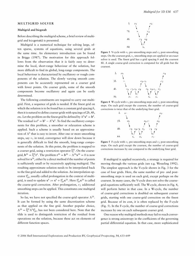
Figure 3 V-cycle with ν1 pre-smoothing steps and ν2 post-smoothingsteps. On the coarsest grid, ν c smoothing steps are applied or an exactsolver is used. The finest grid has a grid spacing h and the coarsest8h. A single coarse-grid correction is computed for all grids but thecoarsest.

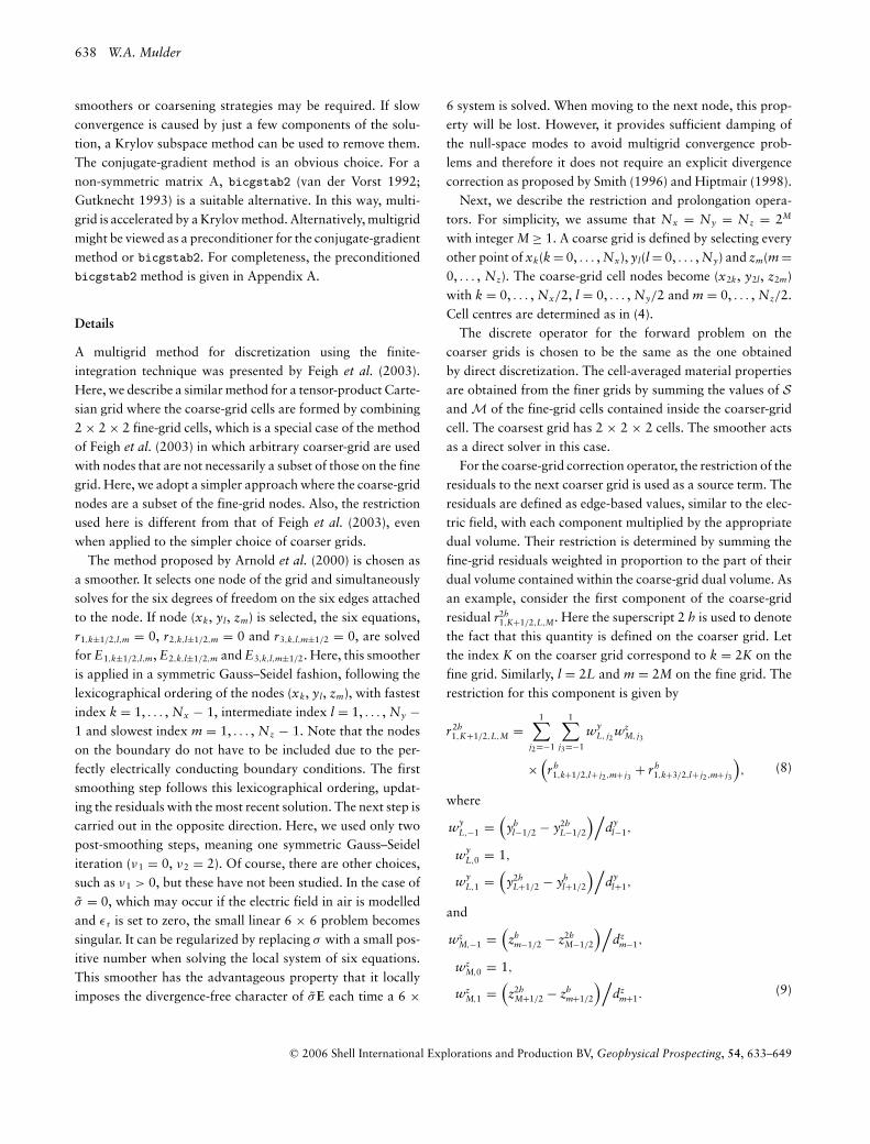
Figure 4 W-cycle with ν1 pre-smoothing steps and ν2 post-smoothingsteps. On each grid except the coarsest, the number of coarse-gridcorrections is twice that of the underlying finer grid.

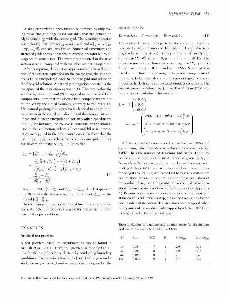
Figure 5 F-cycle with ν1 pre-smoothing steps and ν2 post-smoothingsteps. On each grid except the coarsest, the number of coarse-gridcorrections increases by one compared to the underlying finer grid.

If multigrid is applied recursively, a strategy is required formoving through the various grids (see e.g. Wesseling 1992).The simplest approach is the V-cycle shown in Fig. 3 for thecase of four grids. Here, the same number of pre- and post-smoothing steps is used on each grid, except perhaps on thecoarsest. In many cases, the V-cycle does not solve the coarse-grid equations sufficiently well. The W-cycle, shown in Fig. 4,will perform better in that case. In a W-cycle, the numberof coarse-grid corrections is doubled on subsequent coarsergrids, starting with one coarse-grid correction on the finestgrid. Because of its cost, it is often replaced by the F-cycle(Fig. 5). In the F-cycle, the number of coarse-grid correctionsincreases by one on each subsequent coarser grid.

One reason why multigrid methods may fail to reach conver-gence is strong anisotropy in the coefficients of the governingpartial differential equation. In that case, more sophisticated


638 W.A. Mulder

smoothers or coarsening strategies may be required. If slowconvergence is caused by just a few components of the solu-tion, a Krylov subspace method can be used to remove them.The conjugate-gradient method is an obvious choice. For anon-symmetric matrix A, bicgstab2 (van der Vorst 1992;Gutknecht 1993) is a suitable alternative. In this way, multi-grid is accelerated by a Krylov method. Alternatively, multigridmight be viewed as a preconditioner for the conjugate-gradientmethod or bicgstab2. For completeness, the preconditionedbicgstab2 method is given in Appendix A.

Details

A multigrid method for discretization using the finite-integration technique was presented by Feigh et al. (2003).Here, we describe a similar method for a tensor-product Carte-sian grid where the coarse-grid cells are formed by combining2 × 2 × 2 fine-grid cells, which is a special case of the methodof Feigh et al. (2003) in which arbitrary coarser-grid are usedwith nodes that are not necessarily a subset of those on the finegrid. Here, we adopt a simpler approach where the coarse-gridnodes are a subset of the fine-grid nodes. Also, the restrictionused here is different from that of Feigh et al. (2003), evenwhen applied to the simpler choice of coarser grids.

The method proposed by Arnold et al. (2000) is chosen asa smoother. It selects one node of the grid and simultaneouslysolves for the six degrees of freedom on the six edges attachedto the node. If node (xk, yl, zm) is selected, the six equations,r1,k±1/2,l,m = 0, r2,k,l±1/2,m = 0 and r3,k,l,m±1/2 = 0, are solvedfor E1,k±1/2,l,m, E2,k,l±1/2,m and E3,k,l,m±1/2. Here, this smootheris applied in a symmetric Gauss–Seidel fashion, following thelexicographical ordering of the nodes (xk, yl, zm), with fastestindex k = 1, . . . , Nx − 1, intermediate index l = 1, . . . , Ny −1 and slowest index m = 1, . . . , Nz − 1. Note that the nodeson the boundary do not have to be included due to the per-fectly electrically conducting boundary conditions. The firstsmoothing step follows this lexicographical ordering, updat-ing the residuals with the most recent solution. The next step iscarried out in the opposite direction. Here, we used only twopost-smoothing steps, meaning one symmetric Gauss–Seideliteration (ν1 = 0, ν2 = 2). Of course, there are other choices,such as ν1 > 0, but these have not been studied. In the case ofσ = 0, which may occur if the electric field in air is modelledand ε r is set to zero, the small linear 6 × 6 problem becomessingular. It can be regularized by replacing σ with a small pos-itive number when solving the local system of six equations.This smoother has the advantageous property that it locallyimposes the divergence-free character of σE each time a 6 ×

6 system is solved. When moving to the next node, this prop-erty will be lost. However, it provides sufficient damping ofthe null-space modes to avoid multigrid convergence prob-lems and therefore it does not require an explicit divergencecorrection as proposed by Smith (1996) and Hiptmair (1998).

Next, we describe the restriction and prolongation opera-tors. For simplicity, we assume that Nx = Ny = Nz = 2M

with integer M ≥ 1. A coarse grid is defined by selecting everyother point of xk(k = 0, . . . , Nx), yl(l = 0, . . . , Ny) and zm(m =0, . . . , Nz). The coarse-grid cell nodes become (x2k, y2l, z2m)with k = 0, . . . , Nx/2, l = 0, . . . , Ny/2 and m = 0, . . . , Nz/2.Cell centres are determined as in (4).

The discrete operator for the forward problem on thecoarser grids is chosen to be the same as the one obtainedby direct discretization. The cell-averaged material propertiesare obtained from the finer grids by summing the values of Sand M of the fine-grid cells contained inside the coarser-gridcell. The coarsest grid has 2 × 2 × 2 cells. The smoother actsas a direct solver in this case.

For the coarse-grid correction operator, the restriction of theresiduals to the next coarser grid is used as a source term. Theresiduals are defined as edge-based values, similar to the elec-tric field, with each component multiplied by the appropriatedual volume. Their restriction is determined by summing thefine-grid residuals weighted in proportion to the part of theirdual volume contained within the coarse-grid dual volume. Asan example, consider the first component of the coarse-gridresidual r2h

1,K+1/2,L,M. Here the superscript 2 h is used to denotethe fact that this quantity is defined on the coarser grid. Letthe index K on the coarser grid correspond to k = 2K on thefine grid. Similarly, l = 2L and m = 2M on the fine grid. Therestriction for this component is given by

r2h1,K+1/2,L,M =

1∑j2=−1

1∑j3=−1

wyL, j2

wzM, j3

×(rh

1,k+1/2,l+ j2,m+ j3+ rh

1,k+3/2,l+ j2,m+ j3

), (8)

where

wyL,−1 =

(yh

l−1/2 − y2hL−1/2

)/dy

l−1,

wyL,0 = 1,

wyL,1 =

(y2h

L+1/2 − yhl+1/2

)/dy

l+1,

and

wzM,−1 =

(zh

m−1/2 − z2hM−1/2

)/dz

m−1,

wzM,0 = 1,

wzM,1 =

(z2h

M+1/2 − zhm+1/2

)/dz

m+1.(9)



A simpler restriction operator can be obtained by only tak-ing those fine-grid edge-based variables that are defined onedges coinciding with the coarse grid. The resulting operatorresembles (8), but now wy

L,−1 = wyL,1 = 0 and wy

L,0 = (y2hL+1/2

− y2hL−1/2)/dy

l , and similarly for wz. Numerical experiments onstretched grids showed that this restriction operator led to di-vergence in some cases. The examples presented in the nextsection were all computed with the other restriction operator.

After computing the exact or approximate numerical solu-tion of the discrete equations on the coarse grid, the solutionneeds to be interpolated back to the fine grid and added tothe fine-grid solution. A natural prolongation operator is thetranspose of the restriction operator (8). This means that thesame weights as in (8) and (9) are applied to the electrical fieldcomponents. Note that the electric field components are notmultiplied by their dual volumes, contrary to the residuals.The natural prolongation operator is identical to constant in-terpolation in the coordinate direction of the component, andlinear and bilinear interpolation for two other coordinates.For E1, for instance, the piecewise constant interpolation isused in the x-direction, whereas linear and bilinear interpo-lation are applied in the other coordinates. To show that thenatural prolongation is the same as bilinear interpolation, wecan rewrite, for instance, wz

M,1 in (9) to find

wzM,1 =

(z2h

M+1/2 − zhm+1/2

)/dz

m+1

=12

(z2h

M + z2hM+1

)− 1

2

(zh

m + zhm+1

)12

(zh

m+2 + zhm+1

)− 1

2

(zh

m+1 + zhm

)

= z2hM+1 − zh

m+1

z2hM+1 − z2h

M

,(10)

using m = 2M, z2hM = zh

m, and z2hM+1 = zh

2m+2. The last quotientin (10) reveals the linear weighting for a point zh

m+1 on theinterval [z2h

M , z2hM+1].

In the examples, F-cycles were used for the multigrid itera-tions. A single multigrid cycle was performed when multigridwas used as preconditioner.

E X A M P L E S

Artificial test problem

A test problem based on eigenfunctions can be found inAruliah et al. (2001). Here, this problem is modified to al-low for the use of perfectly electrically conducting boundaryconditions. The domain is � = [0, 2π ]3 m3. Define ψ = sin kx

sin ly sin my, where k, l and m are positive integers. Let the

exact solution be

E1 = a1∂xψ, E2 = a2∂yψ, E3 = a3∂zψ. (11)

The domain � is split into parts �1 for z < π and �2 for z

> π , so that � is the union of their closure. The conductivityis given by σ = σ 0 + σ 1(x + 1)(y + 2)(z − π )2 in �1 andσ = σ 0 in �2. We set ε r = 0, µr = 1 and ω = 106 Hz. Theother parameters are chosen to be a1 = a2 = −2 V, a3 = 1 V,k = l = m = 1, σ 0 = 10 S/m and σ 1 = 1 S/m. Note that ψ isbased on sine functions, causing the tangential components ofthe electric field to vanish at the boundaries in agreement withthe perfectly electrically conducting boundary conditions. Thecurrent source is defined by Js = −σE + ∇ × (iωµ)−1∇ × E,using the exact solution. This results in

Js = −σ

a1∂xψ

a2∂yψ

a3∂zψ

+(iωµ)−1

[l2(a1 − a2) + m2(a1 − a3)

]∂xψ[

k2(a2 − a1) + m2(a2 − a3)]∂yψ[

k2(a3 − a1) + l2(a3 − a2)]∂zψ.

A first series of tests was carried out with σ 0 = 10 S/m andσ 1 = 1 S/m, which avoids zero values for the conductivity.Table 1 lists the number of iterations and errors. The num-ber of cells in each coordinate direction is given by Nx =Ny = Nz = N. For each grid, the number of iterations withmultigrid alone (MG) and with multigrid as preconditionerfor bicgstab2 (bi) is given. Note that bicgstab2 costs moreper iteration because it requires an additional evaluation ofthe residual. Also, each bicgstab2 step is counted as two iter-ations because it involves two multigrid cycles (see AppendixA). Because convergence checks are carried out half-way andat the end of a full iteration step, the method may stop after anodd number of iterations. The iterations were stopped whenthe 2-norm of the residual had dropped by a factor 10−8 fromits original value for a zero solution.

Table 1 Number of iterations and solution errors for the first testproblem with σ 0 = 10 S/m and σ 1 = 1 S/m

N hmax MG bi 2/h2max max/h2

max

16 0.39 7 6 2.0 0.4132 0.20 8 7 2.0 0.4864 0.098 8 7 2.1 0.49

128 0.049 8 6 2.1 0.49


640 W.A. Mulder

The error in the numerical solution is listed in two norms,the 2-norm and the maximum norm. The error for E1 is mea-sured by

2(E1) =[

Nx−1∑k=0

Ny∑l=0

Nz∑m=0

∣∣∣E1,k+1/2,l,m − Eexact1,k+1/2,l,m

∣∣∣2Vk+1/2,l,m

]1/2

,

and similarly for the other components. The maximum erroris

max(E1) = maxk=0,..,Nx−1

maxl=0,...,Ny

maxm=0,...,Nz

∣∣∣E1,k+1/2,l,m − Eexact1,k+1/2,l,m

∣∣∣.Table 1 lists 2 = [

∑3n=1 2(En)2]1/2 and max = maxn=1,2,3

max(En). Note that max does not include scaling by the cor-responding dual volumes. For the exact solution, the point-values at the edge-midpoints were used.

The results in Table 1 show grid-independent convergencefor the multigrid method. The number of iterations withbicgstab2 is smaller, but this is hardly worth the extra costin terms of CPU-time. The errors in the two methods confirmthe second-order accuracy of the solution. The errors were di-vided by the square of the largest cell width hmax, which is themaximum value of hx

k+1/2, hyl+1/2 and hz

m+1/2 on the grid. In thisand the following tables, hmax is given in metres.

Next, the effect of grid stretching was investigated. The gridstretching is carried out in such a way that the ratio betweenneighbouring cell widths in each coordinate is 1 + α whenmoving away from the origin (see power-law stretching in Ap-pendix C). An equidistant grid is obtained for α = 0. Resultsfor grid stretching with α = 0.04 are listed in Table 2. Thegrid-independent convergence rates of the multigrid schemeare apparently lost. The bicgstab2 method is now preferable,as it is able to deal with the slowly converging components ofthe solution. The errors measured by 2 and max confirm thesecond-order accuracy of the solution.

We next considered the problem with σ 0 = 0 S/m, σ 1 =1 S/m and ε r = 0. This implied that we had a vacuum regionfor π < z ≤ 2π . There, the solution is defined up to terms

Table 2 Number of iterations and solution errors for the first testproblem with σ 0 = 10 S/m, σ 1 = 1 S/m and power-law grid stretchingwith α = 0.04


max

16 0.45 8 6 1.9 0.3632 0.26 11 8 1.9 0.3364 0.17 12 14 1.7 0.29

128 0.13 81 32 1.6 0.28

of the form ∇φ. It is reasonable to require the solution tobe of minimum energy. The electric field specified in (11) is,however, not the minimum-norm solution. The latter can beobtained by minimizing

I =3∑

n=1

In, In =∫ 2π

0dx

∫ 2π

0dy

∫ 2π

π

dz |En|2,

where

E = E + ∇φ.

Here,

φ =∑

k′,l ′,m′bk′,l ′,m′ sin k′x sin l ′y sin m′z,

with positive integers k′, l′ and m′. The minimization has to becarried out with respect to bk′,l′,m′ . The minimum is attainedat

bk,l,m = bk,l,m = −k2α1 + l2α2 + m2α3

k2 + l2 + m2(12)

if k = k′, l = l′ and m = m′, whereas bk′,l′,m′ = 0 otherwise.Therefore, the minimum-norm solution is defined by (11) for0 ≤ z < π and by

E1 = (α1 + bk,l,m)∂xψ,

E2 = (α2 + bk,l,m)∂yψ,

E3 = (α3 + bk,l,m)∂zψ,

for π < z ≤ 2π . Recall that ψ = sin kx sin ly sin my. E3 hasa discontinuity at z = π .

Results for this problem are listed in Table 3. The iterativemethods converged rapidly, but the solution errors did not de-crease when the grid was refined. Note that the errors have notbeen multiplied by h−2

max. The cause of the O(1) error behaviour

Table 3 Number of iterations and solution errors for σ 0 = 0 S/m andσ 1 = 1 S/m on the full domain �

N hmax MG bi 2 max

16 0.39 12 0.72 0.169 0.85 0.31

32 0.20 10 0.28 0.108 0.43 0.21

64 0.098 8 0.31 0.117 0.37 0.17

128 0.049 8 0.35 0.136 0.36 0.16



Table 4 Number of iterations and solution errors for σ 0 = 0 S/m andσ 1 = 1 S/m on the domain �1, the part of � where σ > 0


max

16 0.39 12 9 3.6 0.8332 0.20 10 8 4.1 1.264 0.098 8 7 4.2 1.3

128 0.049 8 6 4.2 1.4

Table 5 Number of iterations and solution errors for σ 0 = 0 S/m,σ 1 = 1 S/m and α = 0.04 on the part �1 of the domain where σ

> 0. The number of multigrid iterations performed until the conver-gence stagnates are shown. Despite the stagnation, the solution stillhas second-order behaviour

N hmax MG 2/h2max max/h2

max

16 0.45 (8) 3.0 0.6432 0.26 (8) 2.7 0.6564 0.17 (12) 2.1 0.46

128 0.13 (42) 1.6 0.36

is a solution component in �2 where σ = 0 S/m, that lies in thenull-space of the curl-curl operator. The contribution of thiscomponent can be suppressed by only measuring the errorsin the domain �1 where σ > 0. Results obtained by settingthe errors to zero in �2 are listed in Table 4. The numericalexperiments are the same as in Table 3, so the number of it-erations is identical. Second-order accuracy is now obtained.The null-space component does not apparently affect the ac-curacy of the solution in the part of the domain that has anon-zero conductivity, nor does it affect the convergence rateof the solver. However, the method does not appear to pro-duce the minimum-norm solution where the conductivity iszero.

If the same problem is discretized on a grid with power-lawstretching, we obtain the results given in Table 5. In this case,the multigrid method does not reach convergence. The itera-tions were stopped when the norm of the residual no longerdecreased. The iteration count in brackets is the number of it-erations performed until the convergence stagnates. However,the solutions at stagnation show errors for the subset �1 of thedomain that have second-order accuracy. When bicgstab2

was applied to this problem, it did not reach convergence inless than 2 × 50 iterations.

We conclude that grid stretching is not suitable for the cur-rent problem in terms of convergence speed.

Homogeneous problem with current source

An example that is slightly more realistic from a geophys-ical point of view is a point current source in a homo-geneous formation. We choose the following parameters:ω/2π = 10 Hz, σ = 1 S/m, µr = 1 and ε r = 1. The domain isthe cube [−1, 1] × [−1, 1] × [−1, 1] km3. The current sourceJs = jsδ(x) with js = ( 0 0 1 )T Am is placed at the origin.

The problem is discretized on an equidistant grid withNx = Ny = Nz = N. Power-law grid stretching is used withcell widths increasing away from the source. For the discretesource representation, the adjoint of trilinear interpolation isused. The iterations are stopped if the 2-norm of the residualhas dropped by a factor 10−8 from its initial value for a zerosolution.

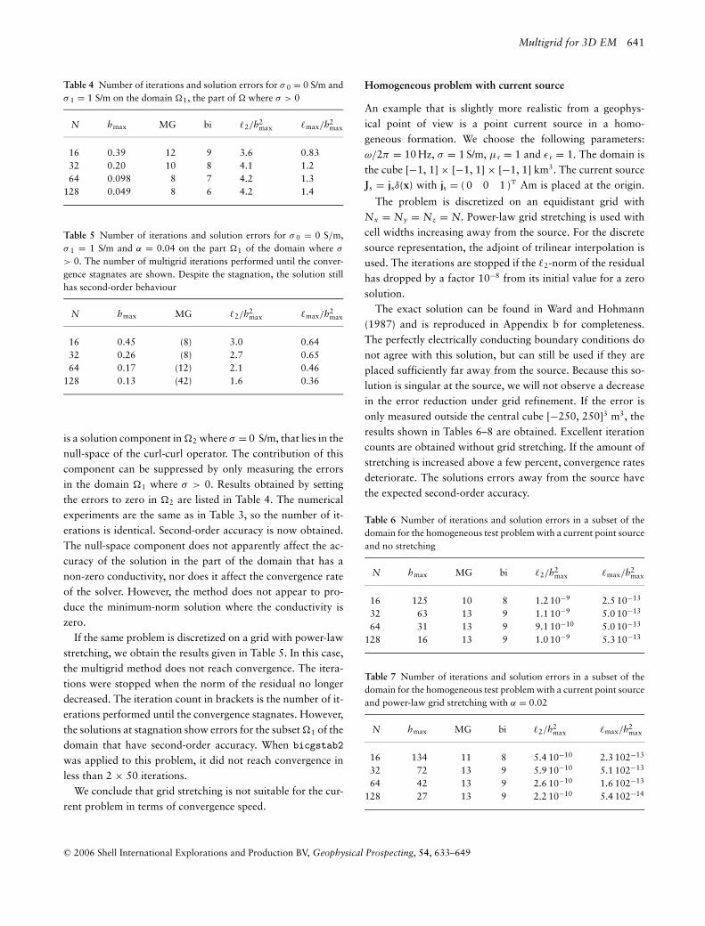
The exact solution can be found in Ward and Hohmann(1987) and is reproduced in Appendix b for completeness.The perfectly electrically conducting boundary conditions donot agree with this solution, but can still be used if they areplaced sufficiently far away from the source. Because this so-lution is singular at the source, we will not observe a decreasein the error reduction under grid refinement. If the error isonly measured outside the central cube [−250, 250]3 m3, theresults shown in Tables 6–8 are obtained. Excellent iterationcounts are obtained without grid stretching. If the amount ofstretching is increased above a few percent, convergence ratesdeteriorate. The solutions errors away from the source havethe expected second-order accuracy.

Table 6 Number of iterations and solution errors in a subset of thedomain for the homogeneous test problem with a current point sourceand no stretching


max

16 125 10 8 1.2 10−9 2.5 10−13

32 63 13 9 1.1 10−9 5.0 10−13

64 31 13 9 9.1 10−10 5.0 10−13

128 16 13 9 1.0 10−9 5.3 10−13

Table 7 Number of iterations and solution errors in a subset of thedomain for the homogeneous test problem with a current point sourceand power-law grid stretching with α = 0.02


max

16 134 11 8 5.4 10−10 2.3 102−13

32 72 13 9 5.9 10−10 5.1 102−13

64 42 13 9 2.6 10−10 1.6 102−13

128 27 13 9 2.2 10−10 5.4 102−14


642 W.A. Mulder

Table 8 Number of iterations and solution errors in a subset of thedomain for the homogeneous test problem with a current point sourceand power-law grid stretching with α = 0.05


max

16 147 11 8 5.0 102−10 2.5 102−13

32 88 14 10 2.2 102−10 1.6 102−13

64 60 26 14 7.7 102−11 2.6 102−14

128 50 185 47 6.6 102−11 5.6 102−15

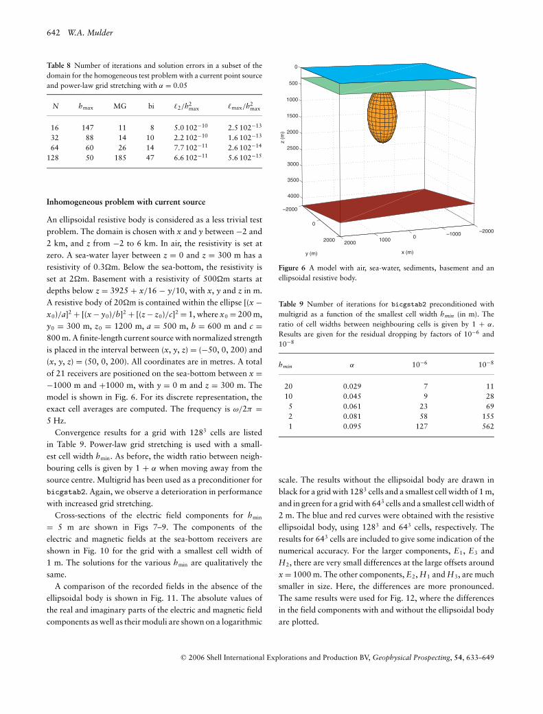
Inhomogeneous problem with current source

An ellipsoidal resistive body is considered as a less trivial testproblem. The domain is chosen with x and y between −2 and2 km, and z from −2 to 6 km. In air, the resistivity is set atzero. A sea-water layer between z = 0 and z = 300 m has aresistivity of 0.3�m. Below the sea-bottom, the resistivity isset at 2�m. Basement with a resistivity of 500�m starts atdepths below z = 3925 + x/16 − y/10, with x, y and z in m.A resistive body of 20�m is contained within the ellipse [(x −x0)/a]2 + [(x − y0)/b]2 + [(z − z0)/c]2 = 1, where x0 = 200 m,y0 = 300 m, z0 = 1200 m, a = 500 m, b = 600 m and c =800 m. A finite-length current source with normalized strengthis placed in the interval between (x, y, z) = (−50, 0, 200) and(x, y, z) = (50, 0, 200). All coordinates are in metres. A totalof 21 receivers are positioned on the sea-bottom between x =−1000 m and +1000 m, with y = 0 m and z = 300 m. Themodel is shown in Fig. 6. For its discrete representation, theexact cell averages are computed. The frequency is ω/2π =5 Hz.

Convergence results for a grid with 1283 cells are listedin Table 9. Power-law grid stretching is used with a small-est cell width hmin. As before, the width ratio between neigh-bouring cells is given by 1 + α when moving away from thesource centre. Multigrid has been used as a preconditioner forbicgstab2. Again, we observe a deterioration in performancewith increased grid stretching.

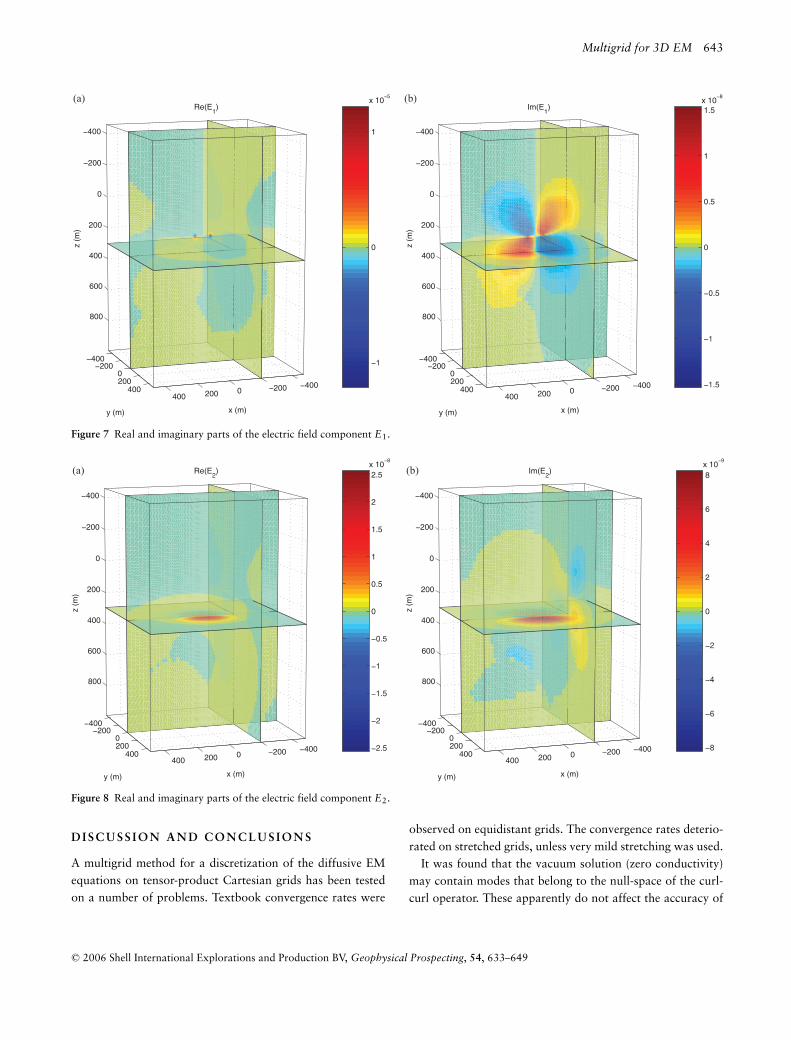
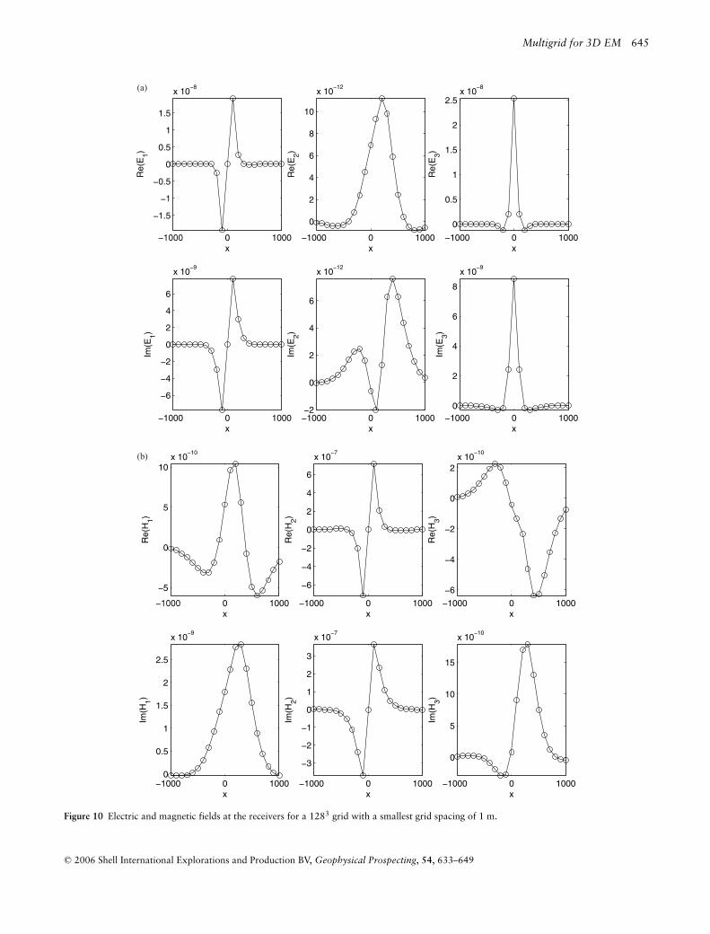
Cross-sections of the electric field components for hmin

= 5 m are shown in Figs 7–9. The components of theelectric and magnetic fields at the sea-bottom receivers areshown in Fig. 10 for the grid with a smallest cell width of1 m. The solutions for the various hmin are qualitatively thesame.

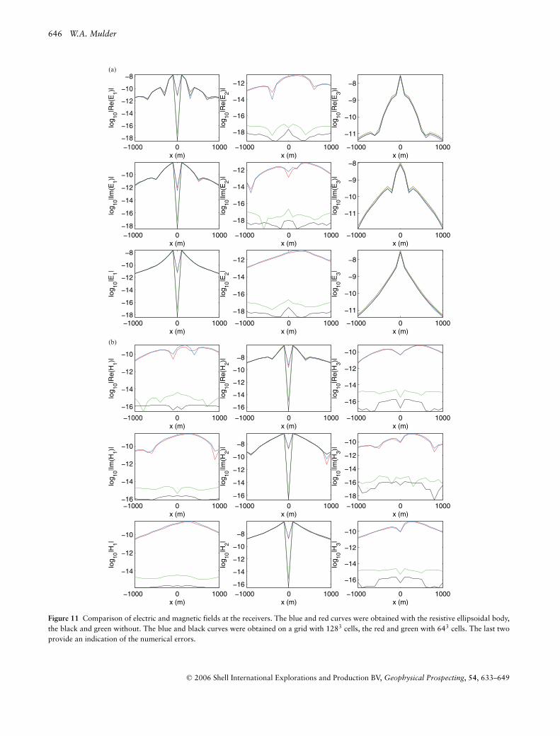
A comparison of the recorded fields in the absence of theellipsoidal body is shown in Fig. 11. The absolute values ofthe real and imaginary parts of the electric and magnetic fieldcomponents as well as their moduli are shown on a logarithmic

–2000–1000010002000

–2000

0

2000

0

500

1000

1500

2000

2500

3000

3500

4000

x (m)y (m)

z (m

)

Figure 6 A model with air, sea-water, sediments, basement and anellipsoidal resistive body.

Table 9 Number of iterations for bicgstab2 preconditioned withmultigrid as a function of the smallest cell width hmin (in m). Theratio of cell widths between neighbouring cells is given by 1 + α.Results are given for the residual dropping by factors of 10−6 and10−8

hmin α 10−6 10−8

20 0.029 7 1110 0.045 9 28

5 0.061 23 692 0.081 58 1551 0.095 127 562

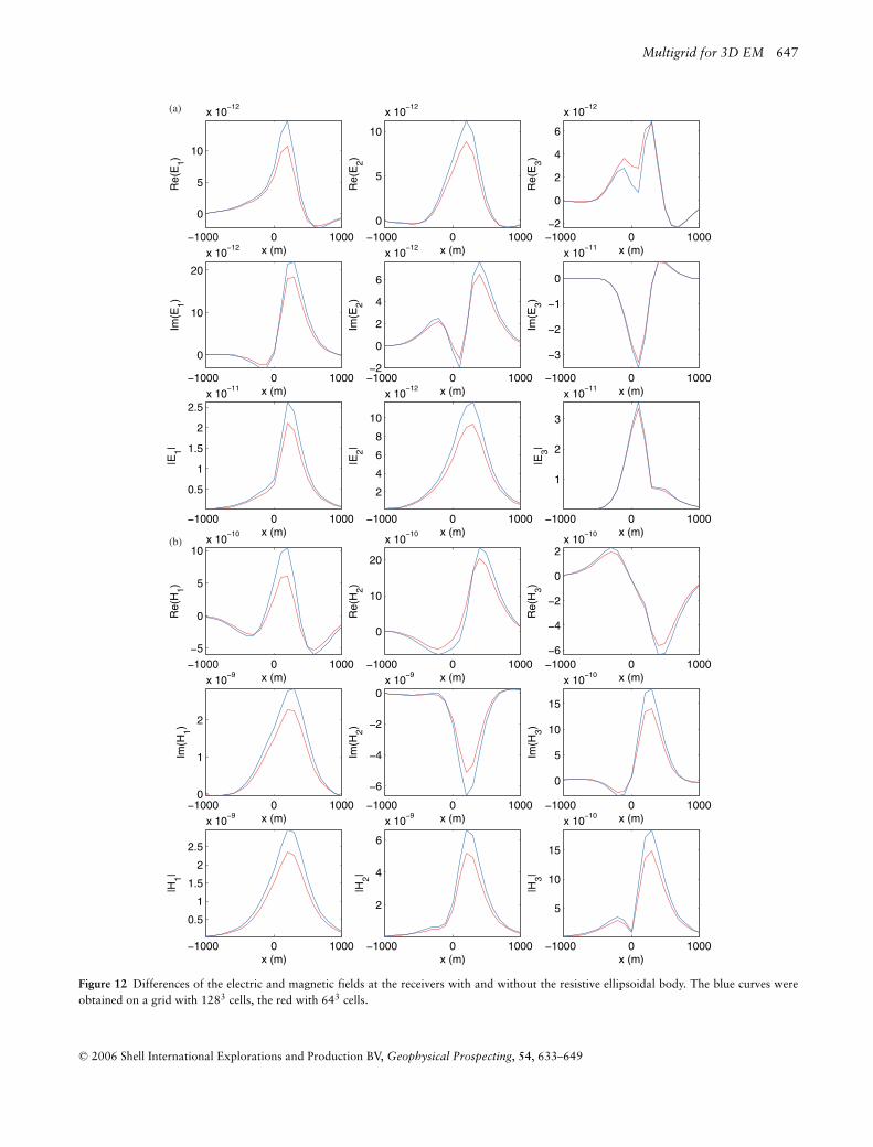
scale. The results without the ellipsoidal body are drawn inblack for a grid with 1283 cells and a smallest cell width of 1 m,and in green for a grid with 643 cells and a smallest cell width of2 m. The blue and red curves were obtained with the resistiveellipsoidal body, using 1283 and 643 cells, respectively. Theresults for 643 cells are included to give some indication of thenumerical accuracy. For the larger components, E1, E3 andH2, there are very small differences at the large offsets aroundx = 1000 m. The other components, E2, H1 and H3, are muchsmaller in size. Here, the differences are more pronounced.The same results were used for Fig. 12, where the differencesin the field components with and without the ellipsoidal bodyare plotted.



0

1

x 105

4002000200400

400200

0200

400

400

200

0

200

400

600

800

x (m)

Re(E1)

y (m)

z (m

)

5

5

0

0.5

1

1.5x 10

8

4002000200400

400200

0200

400

400

200

0

200

400

600

800

x (m)

Im(E1)

y (m)z

(m)

(a) (b)

Figure 7 Real and imaginary parts of the electric field component E1.

5

5

5

0

0.5

1

1.5

2

2.5x 10

8

4002000200400

400200

0200

400

400

200

0

200

400

600

800

x (m)

Re(E2)

y (m)

z (m

)

0

2

4

6

8x 10

9

4002000200400

400200

0200

400

400

200

0

200

400

600

800

x (m)

Im(E2)

y (m)

z (m

)

(a) (b)


D I S C U S S I O N A N D C O N C L U S I O N S

A multigrid method for a discretization of the diffusive EMequations on tensor-product Cartesian grids has been testedon a number of problems. Textbook convergence rates were

observed on equidistant grids. The convergence rates deterio-rated on stretched grids, unless very mild stretching was used.

It was found that the vacuum solution (zero conductivity)may contain modes that belong to the null-space of the curl-curl operator. These apparently do not affect the accuracy of


644 W.A. Mulder

5

0

0.5

1

x 107

4002000200400

400200

0200

400

400

200

0

200

400

600

800

x (m)

Im(E3)

y (m)z

(m)

5

5

0

0.5

1

1.5

x 105

4002000200400

400200

0200

400

400

200

0

200

400

600

800

x (m)

Re(E3)

y (m)

z (m

)

(a) (b)


the solution in the conductive parts of the problem. However,for application in airborne EM, a method that removes thesecomponents needs to be implemented. Alternatively, a verysmall conductivity value can be used.

All the examples employed perfectly electrically conductingboundary conditions. The use of more sophisticated radiationboundary conditions may lead to substantial savings if gridswith less cells can be used.

For equidistant grids, we observed worst-case conver-gence rates of between 0.2 and 0.3 in the 2-norm of theresidual. On stretched grids, the convergence rate deterio-rated considerably. If the grid is stretched, the stretching be-comes more severe on the coarser grids that are used inthe multigrid solver. Stretching the grid has an effect simi-lar to the use of variable coefficients, in this case µ−1

r (x),inside the difference operators. It is well-known that multi-grid methods of the type used here fail if the variable coeffi-cients show large variations from cell to cell or are stronglyanisotropic. There are several potential remedies for thisproblem:� A Krylov subspace method can be used to remove er-

ror components that are slow to reach convergence. Ifthese belong to a low-dimensional space, such an ap-proach will be quite effective. Here, the use of bicgstab2still led to large number of iterations with strongerstretching.

� Line-relaxation, e.g. symmetric line Gauss–Seidel, can beused to remove the effects of strong anisotropy. An examplecan be found in Mulder (1986). For 3D problems, planerelaxation may be required, which is rather costly.

� Semi-coarsening can give the same result. In the standard ap-proach, only one coordinate of the grid is coarsened at thetime. A scheme that uses all directs simultaneously was in-troduced by Mulder (1989). An advantage of this approachis that very simple relaxation schemes, such as Point–Jacobi,can be used. Whether or not this is true for the present prob-lem with the large curl-curl null-space remains to be seen.

� The adverse effects of strongly varying coefficients can bereduced by using operator-weighted restriction and prolon-gation operators (Wesseling 1992).

� Another approach is to define a coarser grid differently, forinstance by not coarsening cells if they have large widthsrelative to the smallest cell (Poplau and van Rienen 2001),or by using coarser grids with nodes that do not coincidewith the finer grid (Feigh et al. 2003).

� An alternative is the computer-science solution of localgrid refinement on equidistant grids. This should givevery good convergence rates while still allowing for finergrids, where necessary, at the expense of increased codecomplexity.

All of these remedies, except perhaps the last, will result ina method that will be more costly than the present one. An



0 1000

5

5

0

0.5

1

1.5

x 108

x

Re(

E1)

1000 0 1000

6

4

2

0

2

4

6

x 109

x

Im(E

1)

1000 0 1000

0

2

4

6

8

10

x 1012

x

Re(

E2)

1000 0 10002

0

2

4

6

x 1012

x

Im(E

2)

1000 0 1000

0

0.5

1

1.5

2

2.5x 10

8

x

Re(

E3)

1000 0 10000

2

4

6

8

x 109

xIm

(E3)

0 1000

0

5

10x 10

10

x

Re(

H1)

1000 0 10000

0.5

1

1.5

2

2.5

x 109

x

Im(H

1)

1000 0 1000

6

4

2

0

2

4

6

x 107

x

Re(

H2)

1000 0 1000

3

2

1

0

1

2

3

x 107

x

Im(H

2)

1000 0 1000

6

4

2

0

2x 10

10

x

Re(

H3)

1000 0 1000

0

5

10

15

x 1010

x

Im(H

3)

(a)

(b)

Figure 10 Electric and magnetic fields at the receivers for a 1283 grid with a smallest grid spacing of 1 m.


646 W.A. Mulder

0 1000x (m)

log 10

|Re(

H1)|

1000 0 100016

14

12

10

x (m)

log 10

|Im(H

1)|

1000 0 1000

14

12

10

x (m)

log 10

|H1|

1000 0 1000

16

14

12

10

8

x (m)

log 10

|Re(

H2)|

1000 0 1000

16

14

12

10

8

x (m)

log 10

|Im(H

2)|

1000 0 100016

14

12

10

8

x (m)

log 10

|H2|

1000 0 1000

16

14

12

10

x (m)

log 10

|Re(

H3)|

1000 0 100018

16

14

12

10

x (m)

log 10

|Im(H

3)|

1000 0 1000

16

14

12

10

x (m)

log 10

|H3|

0 1000x (m)

log 10

|Re(

E1)|

1000 0 100018

16

14

12

10

x (m)

log 10

|Im(E

1)|

1000 0 100018

16

14

12

10

8

x (m)

log 10

|E1|

1000 0 1000

18

16

14

12

x (m)

log 10

|Re(

E2)|

1000 0 1000

18

16

14

12

x (m)

log 10

|Im(E

2)|

1000 0 1000

18

16

14

12

x (m)

log 10

|E2|

1000 0 1000

11

10

9

8

x (m)

log 10

|Re(

E3)|

1000 0 1000

11

10

9

8

x (m)

log 10

|Im(E

3)|

1000 0 1000

11

10

9

8

x (m)lo

g 10|E

3|

(a)

(b)

Figure 11 Comparison of electric and magnetic fields at the receivers. The blue and red curves were obtained with the resistive ellipsoidal body,the black and green without. The blue and black curves were obtained on a grid with 1283 cells, the red and green with 643 cells. The last twoprovide an indication of the numerical errors.



0 1000

0

5

10

x 1012

x (m)

Re(

E1)

1000 0 1000

0

10

20

x 1012

x (m)

Im(E

1)

1000 0 1000

0.5

1

1.5

2

2.5x 10

11

x (m)

|E1|

1000 0 1000

0

5

10

x 1012

x (m)

Re(

E2)

1000 0 10002

0

2

4

6

x 1012

x (m)

Im(E

2)

1000 0 1000

2

4

6

8

10

x 1012

x (m)

|E2|

1000 0 10002

0

2

4

6

x 1012

x (m)

Re(

E3)

1000 0 1000

3

2

1

0

x 1011

x (m)

Im(E

3)1000 0 1000

1

2

3

x 1011

x (m)|E

3|

0 1000

0

5

10x 10

10

x (m)

Re(

H1)

1000 0 10000

1

2

x 109

x (m)

Im(H

1)

1000 0 1000

0.5

1

1.5

2

2.5

x 109

x (m)

|H1|

1000 0 1000

0

10

20

x 1010

x (m)

Re(

H2)

1000 0 1000

6

4

2

0x 10

9

x (m)

Im(H

2)

1000 0 1000

2

4

6

x 109

x (m)

|H2|

1000 0 10006

4

2

0

2x 10

10

x (m)

Re(

H3)

1000 0 1000

0

5

10

15

x 1010

x (m)

Im(H

3)

1000 0 1000

5

10

15

x 1010

x (m)

|H3|

(a)

(b)

Figure 12 Differences of the electric and magnetic fields at the receivers with and without the resistive ellipsoidal body. The blue curves wereobtained on a grid with 1283 cells, the red with 643 cells.


648 W.A. Mulder

investigation into which is the most cost-effective still has tobe carried out.

Finally, it should be noted that only a few options for the re-striction, prolongation, relaxation and coarse-grid operatorshave been investigated. Other choices may or may not im-prove the convergence rates. For instance, material propertieson edges and faces were determined here by averaging theirgiven values in neighbouring cells. Conceptually, these aver-ages might be determined directly for a given model and alsobe used for the construction of the coarse-grid operator. Othersmoothers such as Red-Black (checkerboard) relaxation couldbe considered. The block Gauss–Seidel method used here is agood solver but may, in fact, not be the best smoother.

R E F E R E N C E S

Arnold D.N., Falk R.S. and Winther R. 2000. Multigrid in H(div) andH(curl). Numerische Mathematik 85, 197–217.

Aruliah D.A. and Ascher U.M. 2003. Multigrid preconditioning forKrylov methods for time-harmonic Maxwell’s equations in 3D.SIAM Journal on Scientific Computing 24, 702–718.

Aruliah D.A., Ascher U.M., Haber E. and Oldenburg D. 2001. Amethod for the forward modelling of 3D electromagnetic quasi-static problems. Mathematical Models and Methods in Applied Sci-ences 11, 1–21.

Briggs W.L. 1987. A Multigrid Tutorial. Society for Industrial andApplied Mathematics, Philadelphia, USA. ISBN 0898712211.

Clemens M. and Weiland T. 2001. Discrete electromagnetism with theFinite Integration Technique. Progress in Electromagnetic Research(PIER) 32, 65–87.

Feigh S., Clemens M. and Weiland T. 2003. Geometric multigridmethod for electro- and magnetostatic field simulation using theconformal finite integration technique. 2003 Copper MountainConference on Multigrid Methods, Copper Mountain, Colorado,USA. (http://www.mgnet.org/mgnet-cm2003.html).

George A. and Liu J. 1981. Computer Solution of Large Sparse Posi-tive Definite Systems. Prentice–Hall Inc. ISBN 0131652745.

Gutknecht M.H. 1993. Variants of BiCGStab for matrices with com-plex spectrum. SIAM Journal on Scientific and Statistical Comput-ing 14, 1020–1033.

Haber E. and Ascher U.M. 2001. Fast finite volume simulation of 3Delectromagnetic problems with highly discontinuous coefficients.SIAM Journal on Scientific and Statistical Computing 22, 1943–1961.

Hiptmair R. 1998. Multigrid method for Maxwell’s equations. SIAMJournal on Numerical Analysis 36, 204–225.

Monk P. and Suli E. 1994. A convergence analysis of Yee’s scheme onnonuniform grids. SIAM Journal on Numerical Analysis 31, 393–412.

Mulder W.A. 1986. Computation of the quasi-steady gas flow in aspiral galaxy by means of a multigrid method. Astronomy and As-trophysics 156, 354–380.

Mulder W.A. 1989. A new multigrid approach to convection prob-lems. Journal of Computational Physics 83, 303–323.

Poplau G. and van Rienen U. 2001. Multigrid solvers for Poisson’sequation in computational electromagnetics. In: Scientific Comput-ing in Electrical Engineering (eds U. van Rienen, M. Gunther and D.Hecht), Lecture Notes in Computational Science and Engineering18, pp. 169–176. Springer Verlag, Inc. ISBN 3540421734.

Smith J.T. 1996. Conservative modeling of 3-D electromagnetic fields,Part II: Biconjugate gradient solver and an accelerator. Geophysics61, 1319–1324.

van der Vorst H.A. 1992. BI-CGSTAB: a fast and smoothly convergingvariant of bi-CG for the solution of nonsymmetric linear systems.SIAM Journal on Scientific and Statistical Computing 13, 631–644.

Ward S.H. and Hohmann G.W. 1987. Electromagnetic theory forgeophysical applications. In: Electromagnetic Methods in AppliedGeophysics – Theory, Vol. 1 (ed. M.N. Nabighian), pp. 131–311.Society of Exploration Geophysicists.

Weiland T. 1977. A discretization method for the solution ofMaxwell’s equations for six-components fields. Electronics andCommunications 31, 116–120.

Wesseling P. 1992. An Introduction to Multigrid Methods. John Wiley& Sons, Inc. ISBN 0471930830.

Yee K. 1966. Numerical solution of initial boundary value problemsinvolving Maxwell’s equations in isotropic media. IEEE Transac-tions on Antennas and Propagation 16, 302–307.

A P P E N D I X A

Preconditioned bicgstab

The problem is find the solution x that leads to a zero residualr = b − Ax. The preconditioner is M.

Compute the residual r0 = b − Ax0 for a starting value x0.Set p0 = r0. Choose an arbitrary r0 such that rH0 r0 = 0, forinstance r0 = r0. Here aH denotes the conjugate transpose ofa, so that aHb is a scalar product. This product is the conjugateof the usual complex scalar product (a, b). Set ρ0 = 1 andγ 0 = 1.

For k = 0, 1, . . . until convergence do:

pk = M−1pk,

vk = Apk,

ρk+1 = rH0 rk,

αk = ρk+1

rH0 vk,

xk+1/2 = xk + αkpk,

sk = rk − αkvk,

sk = M−1sk,

wk = Ask,

γk = wHk sk

wHk wk

,



xk+1 = xk+1/2 + γksk,

rk+1 = sk − γkwk,

βk = αk

γk

ρk+1

ρk,

pk+1 = rk + βk(pk − γkvk).

Convergence checks are carried out, once either xk+1/2 or xk+1

becomes available, by comparing the norm of b − Ax to thenorm of b times the convergence tolerance.

The algorithm requires two calls to the multigrid solver(M−1). The computations of the form Ax can be carriedout matrix-free by evaluating the spatial discretization. Thereare three of these. Together with the residual evaluationsrequired for the convergence checks, they add to the costof two multigrid iterations. Nevertheless, we have countedone full bicgstab2 iteration as two iterations when com-paring it with multigrid alone. Convergence checks are car-ried out after each solution update, i.e. once xk+1/2 and xk+1

become available, at the expense of an additional residualcomputation.

A P P E N D I X B

Exact solution for the homogeneous case

The solution for the electric case with constant material prop-erties is (Ward and Hohmann 1987)

E = σ−1[k2A + ∇(∇ · A)

],

H = ∇ × A,

A = jseikr/(4πr ),

where r = ||x − xs||, k2 = iωµσ and

k2A + �A = −Js = −jsδ(x − xs).

This leads to

E = 14πr5σ

eikr h,

h = (k2r2 + ikr − 1)r2js − (k2r2 + 3ikr − 3)(x′ · js)x′,

where x′ = x − xs and

H = eikr

4πr3(1 − ikr ) (js × x′).

Remark: js represents a vector of electric dipoles (see Wardand Hohmann 1987, p. 173) with strength measured by cur-rent times its (infinitesimal) length.

A P P E N D I X C

Power-law grid stretching

Let the grid start at x = xmin and end at x = xmax. The gridis stretched with respect to some reference point x0 inside thedomain. There are nL cells to the left of x0 and nR to the right,with a total of n = nL + nR cells. The grid spacings or cellwidths are given by

hk = h a(nL−1−k), for k = 0, . . . , nL − 1,

hk = h a(k−nL), for k = nL, . . . , n − 1.

Here a = 1 + α. After summation, we have

anR − 1a − 1

= (xmax − x0)/h,anL − 1a − 1

= (x0 − xmin)/h.

To determine nL and nR = n − nL, we determine the smallestinteger nL that minimizes the term,∣∣∣(a(n−nL) − 1

)/(anL − 1) − r

∣∣∣,where

r = (xmax − x0)/(x0 − xmin).

h is then determined such that∑n−1

k=0 hk = xmax − xmin.


Documents

A multigrid solver for 3D electromagnetic diffusion