A parallel multigrid Poisson solver for ﬂuids …pages.cs.wisc.edu/~sifakis/papers/mgpcg_poisson.pdf · A parallel multigrid Poisson solver for ... introduced a higher-order parallel

Eurographics/ ACM SIGGRAPH Symposium on Computer Animation (2010)M. Otaduy and Z. Popovic (Editors)

A parallel multigrid Poisson solver for fluids simulation onlarge grids

A. McAdams1,2, E. Sifakis1,3, and J. Teran1,3

1University of California, Los Angeles2Weta Digital 3Walt Disney Animation Studios

AbstractWe present a highly efficient numerical solver for the Poisson equation on irregular voxelized domains supportingan arbitrary mix of Neumann and Dirichlet boundary conditions. Our approach employs a multigrid cycle asa preconditioner for the conjugate gradient method, which enables the use of a lightweight, purely geometricmultigrid scheme while drastically improving convergence and robustness on irregular domains. Our method isdesigned for parallel execution on shared-memory platforms and poses modest requirements in terms of bandwidthand memory footprint. Our solver will accommodate as many as 7682×1152 voxels with a memory footprint lessthan 16GB, while a full smoke simulation at this resolution fits in 32GB of RAM. Our preconditioned conjugategradient solver typically reduces the residual by one order of magnitude every 2 iterations, while each PCGiteration requires approximately 6.1sec on a 16-core SMP at 7683 resolution. We demonstrate the efficacy of ourmethod on animations of smoke flow past solid objects and free surface water animations using Poisson pressureprojection at unprecedented resolutions.

Categories and Subject Descriptors (according to ACM CCS): I.3.7 [Computer Graphics]: Three-DimensionalGraphics and Realism—Animation; G.1.8 [Numerical Analysis]: Finite difference methods—Multigrid and mul-tilevel methods

1. Introduction

Incompressible flows have proven very effective at generat-ing many compelling effects in computer graphics includ-ing free surface, multiphase and viscoelastic fluids, smokeand fire. One of the most popular techniques for enforcingthe incompressibility constraint is MAC grid based projec-tion as pioneered by [HW65]. They showed that for sim-ulations on a regular Cartesian lattice, staggering velocitycomponents on cell faces and pressures at cell centers givesrise to a natural means for projecting such a staggered ve-locity field to a discretely divergence free counterpart. Thisprojection is ultimately accomplished by solving a Poissonequation for the cell centered pressures. Categorization ofthe Cartesian domain into air, fluid or solid cells gives riseto what [BBB07] describe as the “voxelized Poisson equa-tion” with unknown pressures and equations at each fluidcell, Dirichlet boundary conditions in each air cell and Neu-mann boundary conditions at faces separating fluid and solid

cells. This technique for enforcing incompressibility viavoxelized Poisson was originally popularized in computergraphics by [FM96] who used Successive Over Relaxation(SOR) to solve the system. [FF01] later showed that incom-plete Cholesky preconditioned conjugate gradient (ICPCG)was more efficient. This has since become a very widelyadopted approach for voxelized Poisson and has been usedfor smoke [SRF05,MTPS04,FSJ01] and fire [HG09] as wellas continuum models for solids such as sand [ZB05] andhair [MSW∗09]. The voxelized pressure Poisson equationis also popular in free surface flows due to its efficiency andrelative simplicity [CMT04,FF01,GBO04,HK05,HLYK08,KC07, MTPS04, NNSM07, WMT05, ZB05]. There are al-ternatives to voxelized Poisson, e.g., [BBB07] used a vari-ational approach that retains the same sparsity of discretiza-tion while improving behavior on coarse grids for bothsmoke and free surface. Also, many non-MAC grid basedapproaches have been used to enforce incompressibility, typ-ically for smoke rather than free surface simulations. For ex-

c© The Eurographics Association 2010.

McAdams et al. / A parallel multigrid Poisson solver for fluids simulation on large grids

ample, [MCP∗09,KFCO06,FOK05,ETK∗07] use conform-ing tetrahedralizations to accurately enforce boundary con-ditions, [LGF04] uses adaptive octree-based discretization,and [CFL∗07] makes use of tetrahedralized volumes for freesurface flow.

Incomplete Cholesky preconditioned CG remains thestate of the art for voxelized Poisson. Although ICPCG cer-tainly offers an acceleration over unpreconditioned CG, itis still impractical at high resolutions since the requirednumber of iterations increases drastically with the size ofthe problem, and the cost of updating and explicitly storingthe preconditioner is very high for large domains. Further-more, since ICPCG involves sparse back-substitution, it can-not be parallelized without further modification [HGS∗07].Whereas multigrid methods have the potential for constantasymptotic convergence rates, our purely geometric multi-grid preconditioned conjugate gradient algorithm is the firstin the graphics literature to demonstrate these convergencerates on the highly irregular voxelized domains common tofree surface simulation.

Our main contributions

We handle an arbitrary mix of Dirichlet and Neumannboundary conditions on irregular voxelized domains com-mon to free surface flow simulations. Previous worksproposing geometric multigrid methods for rectangular do-mains [TO94, AF96, BWRB05, BWKS06, KH08], as wellas irregular Neumann boundaries (via a projection method)[MCPN08], cannot handle this general case.

We use a purely geometric, matrix-free formulation andmaintain constant convergence rates, regardless of bound-ary geometry. [BWRB05] presents a lightweight, matrix-free geometric multigrid method for uniform rectangular do-mains; however, extension to voxelized domains has provedchallenging. In fact, [HMBVR05] chose a cut-cell embed-ded boundary discretization, citing non-convergence on thevoxelized Poisson discretization due to instabilities at irreg-ular boundaries. Even higher order embeddings do not en-sure constant convergence as noted by [CLB∗09], wherethey solve the Poisson equation on a surface mesh embed-ded in a background lattice: they noticed convergence dete-rioration when the coarse grid could not resolve the mesh.Furthermore, a number of works have opted to use the moregeneral algebraic multigrid, despite its significantly greaterset-up costs and difficult to parallelize nature [TOS01], dueto the challenges of finding a convergent geometric solu-tion [CFL∗07, CGR∗04, PM04].

In comparison to widely-used ICPCG solvers, our methodrequires less storage, is more convergent, and more paral-lelizable. Unlike ICPCG, no preconditioning matrices areexplicitly stored. This allows us to accommodate as manyas 7682×1152 voxels with less than 16GB of memory.Whereas ICPCG requires sparse backsubstition and cannot

be parallelized without significant modifications, this is notthe case for our solver. Finally, we demonstrate that oursolver is significantly faster than ICPCG on moderately sizedproblems, and our convergence rates are independent of gridsize, so this performance comparison improves with resolu-tion. As a result, we can solve (with residual reduction bya factor of 104) at 1283 resolution in less than 0.75 secondsand 7683 resolution in about a minute.

2. Related Work

Multigrid methods have proven effective for a number of ap-plications in graphics including image processing [KH08,BWKS06, RC03], smoke simulation [MCPN08], mesh de-formation [SYBF06], thin shells [GTS02], cloth simula-tion [ONW08], fluid simulation [CFL∗07, CTG10], ge-ometry processing [NGH04], deformable solids simula-tion [OGRG07], rendering [Sta95, HMBVR05], and havebeen efficiently ported to the GPU [BFGS03, GWL∗03,GSMY∗08]. While the majority of works in this area ei-ther focused on rectangular domains or algebraic multigridformulations on irregular geometries, there are some no-table geometric multigrid solutions for irregular domains.[HMBVR05] and [CLB∗09] embed their irregular geome-try into regular lattices, producing irregular stencils. [RC03,ONW08] use a coarse-to-fine geometric hierarchy which en-sures mesh alignment across levels, but these methods re-quire the geometry to be fully resolved at the coarsest leveland thus are impractical for resolving fine fluid features.[SAB∗99] show that using multigrid as a preconditioner toCG rather rather than a stand-alone solver can alleviate in-stability issues on some problems. Multigrid preconditionedCG for the Poisson equation on rectangular grids can befound in [Tat93] and the algorithm is parallelized in [TO94]and later [AF96]. [KH08] introduced a higher-order parallelmultigrid solver for large rectangular images.

3. Method overview

We wish to solve the Poisson boundary value problem:

∆p = f in Ω⊂ R3 (1)

p(x) = α(x) on ΓD, pn(x) = β(x) on ΓN

where the boundary of the domain ∂Ω = ΓD ∩ΓN is parti-tioned into the disjoint subsets ΓD and ΓN where Dirichletand Neumann conditions are imposed, respectively. For flu-ids simulations, Ω corresponds to the body of water, whileDirichlet boundary conditions are imposed on the air-waterinterface and Neumann conditions at the surfaces of con-tact between the fluid and immersed objects (or the walls ofa container). Without loss of generality we will assume thatthe Neumann condition is zero (β(x)=0) since non-zero con-ditions can be expressed by modifying the right hand side.



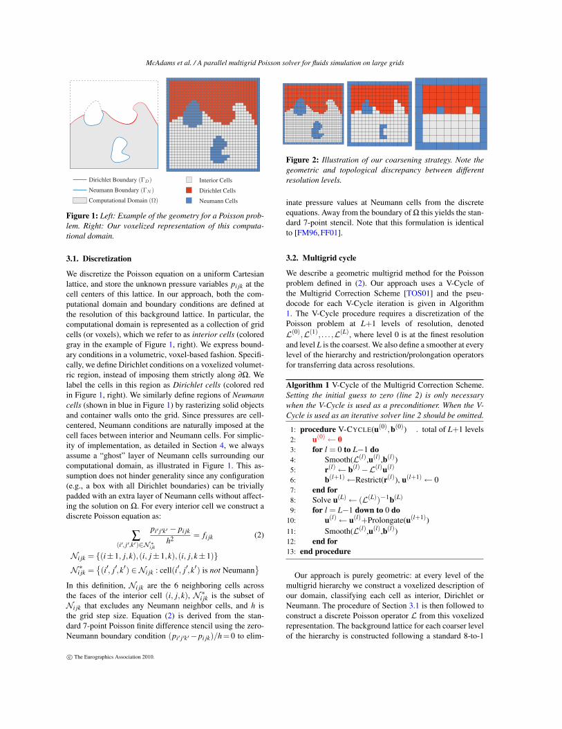
Figure 1: Left: Example of the geometry for a Poisson prob-lem. Right: Our voxelized representation of this computa-tional domain.

3.1. Discretization

We discretize the Poisson equation on a uniform Cartesianlattice, and store the unknown pressure variables pi jk at thecell centers of this lattice. In our approach, both the com-putational domain and boundary conditions are defined atthe resolution of this background lattice. In particular, thecomputational domain is represented as a collection of gridcells (or voxels), which we refer to as interior cells (coloredgray in the example of Figure 1, right). We express bound-ary conditions in a volumetric, voxel-based fashion. Specifi-cally, we define Dirichlet conditions on a voxelized volumet-ric region, instead of imposing them strictly along ∂Ω. Welabel the cells in this region as Dirichlet cells (colored redin Figure 1, right). We similarly define regions of Neumanncells (shown in blue in Figure 1) by rasterizing solid objectsand container walls onto the grid. Since pressures are cell-centered, Neumann conditions are naturally imposed at thecell faces between interior and Neumann cells. For simplic-ity of implementation, as detailed in Section 4, we alwaysassume a “ghost” layer of Neumann cells surrounding ourcomputational domain, as illustrated in Figure 1. This as-sumption does not hinder generality since any configuration(e.g., a box with all Dirichlet boundaries) can be triviallypadded with an extra layer of Neumann cells without affect-ing the solution on Ω. For every interior cell we construct adiscrete Poisson equation as:

∑(i′, j′,k′)∈N∗i jk

pi′ j′k′ − pi jk

h2 = fi jk (2)

Ni jk = (i±1, j,k),(i, j±1,k),(i, j,k±1)

N ∗i jk =(i′, j′,k′) ∈Ni jk : cell(i′, j′,k′) is not Neumann

In this definition, Ni jk are the 6 neighboring cells acrossthe faces of the interior cell (i, j,k), N ∗i jk is the subset ofNi jk that excludes any Neumann neighbor cells, and h isthe grid step size. Equation (2) is derived from the stan-dard 7-point Poisson finite difference stencil using the zero-Neumann boundary condition (pi′ j′k′−pi jk)/h = 0 to elim-

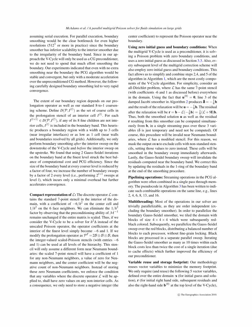
Figure 2: Illustration of our coarsening strategy. Note thegeometric and topological discrepancy between differentresolution levels.

inate pressure values at Neumann cells from the discreteequations. Away from the boundary of Ω this yields the stan-dard 7-point stencil. Note that this formulation is identicalto [FM96, FF01].

3.2. Multigrid cycle

We describe a geometric multigrid method for the Poissonproblem defined in (2). Our approach uses a V-Cycle ofthe Multigrid Correction Scheme [TOS01] and the pseu-docode for each V-Cycle iteration is given in Algorithm1. The V-Cycle procedure requires a discretization of thePoisson problem at L+1 levels of resolution, denotedL(0),L(1), . . . ,L(L), where level 0 is at the finest resolutionand level L is the coarsest. We also define a smoother at everylevel of the hierarchy and restriction/prolongation operatorsfor transferring data across resolutions.

Algorithm 1 V-Cycle of the Multigrid Correction Scheme.Setting the initial guess to zero (line 2) is only necessarywhen the V-Cycle is used as a preconditioner. When the V-Cycle is used as an iterative solver line 2 should be omitted.

1: procedure V-CYCLE(u(0),b(0)) . total of L+1 levels2: u(0)← 03: for l = 0 to L−1 do4: Smooth(L(l),u(l),b(l))5: r(l)← b(l)−L(l)u(l)

6: b(l+1)←Restrict(r(l)), u(l+1)← 07: end for8: Solve u(L)← (L(L))−1b(L)

9: for l = L−1 down to 0 do10: u(l)← u(l)+Prolongate(u(l+1))11: Smooth(L(l),u(l),b(l))12: end for13: end procedure

Our approach is purely geometric: at every level of themultigrid hierarchy we construct a voxelized description ofour domain, classifying each cell as interior, Dirichlet orNeumann. The procedure of Section 3.1 is then followed toconstruct a discrete Poisson operator L from this voxelizedrepresentation. The background lattice for each coarser levelof the hierarchy is constructed following a standard 8-to-1



cell coarsening procedure, generating a grid with twice thestep size. Our hierarchy is deep: the coarsest level is typically8× 8× 8. The coarse grid is positioned in such a way thatthe bounding box of the domain, excluding the ghost layerof Neumann cells, aligns with cell boundaries at both resolu-tions (see Figure 2). A coarse cell will be labeled Dirichlet, ifany of its eight fine children is a Dirichlet cell. If none of theeight children is a Dirichlet cell, but at least one is interior,then the coarse cell will be labeled as interior. Otherwise,the coarse cell is labeled Neumann. As seen in Figure 2 thiscoarsening strategy can create significant geometric discrep-ancies when fine grid features are not resolved on the coarse,and even change the topology of the domain, e.g., Neumannbubbles are eventually absorbed into the interior region, andthin interior features are absorbed into the Dirichlet region.The impact of this discrepancy is addressed later in this sec-tion.

We construct the restriction operator as the tensor productstencilR=B⊗B⊗B, where B is a 1D stencil with 4 pointsgiven by:

(Buh)(x) = 18 uh(x− 3h

2 )+ 38 uh(x− h

2 )+

+ 38 uh(x+ h

2 )+ 18 uh(x+ 3h

2 ) = u2h(x)

Figure 3 (left) illustrates the 2D analogue of this tensor prod-uct stencil, spanning 16 points (compared to 64, in 3D). Notethat since our variables are cell centered, the coarse grid vari-ables will not coincide with a subset of the fine variables.The prolongation operator is defined by PT =8B⊗B⊗B,i.e., a scaled transposition of the restriction operator. We canverify that the prolongation is exactly a trilinear interpola-tion operator from the coarse to the fine grid variables. Welimit the output of the prolongation and restriction opera-tors to interior cell variables only; therefore, we only restrictinto interior coarse cells, and only prolongate into interiorfine variables. Conversely, if a restriction/prolongation sten-cil uses a non-interior cell variable as input, we substitute azero value instead.

Our smoother of choice is the damped Jacobi method withparameter ω = 2/3 (see Algorithm 2), which is known to bestable for the Poisson equation and facilitates parallelismbetter than Gauss-Seidel methods. For problems with mixedboundary conditions and irregular domain geometries it iscommon practice to perform additional smoothing near theboundary of the computational domain. Consequently, wedefine a boundary region consisting of interior cells withina certain distance of Dirichlet or Neumann cells. Figure 3(right) illustrates the boundary region (shaded black) withina radius of 2 of non-interior cells (measured by L1-distance).In our approach, we perform a number of Gauss-Seidel iter-ations (see Algorithm 2, bottom) on the boundary region inaddition to the damped Jacobi smoother applied on the entiredomain. Our complete smoothing procedure will start withM Gauss-Seidel sweeps on the boundary region, continuewith a damped Jacobi sweep over the entire domain, and fin-

Figure 3: Left: 2D illustration of the restriction operator.Right: Illustration of the boundary region. A band width of 2is pictured.

ish with another N Gauss-Seidel boundary sweeps. Finally,we can approximate the exact solution for the coarsest levelin the hierarchy by simply iterating the smoothing procedurea large number of times.

Algorithm 2 Damped Jacobi (ω = 2/3) and Gauss-SeidelSmoothers

1: procedure DAMPEDJACOBISMOOTH(L,u,b,I)2: foreach I = (i, j,k) ∈ I do . I is set of cell indices3: δI ← (bI−LIu)/LII. LI is the equation in cell I4: foreach I = (i, j,k) ∈ I do5: uI += 2

3 δI . δδδ is an auxiliary variable6: end procedure7: procedure GAUSSSEIDELSMOOTH(L,u,b,I)8: foreach I = (i, j,k) ∈ I do9: uI += (bI−LIu)/LII

10: end procedure

The multigrid scheme we just described is particularlysimplistic, using an elementary coarsening strategy, a verybasic smoother and without specialized transfer operatorsnear the boundary. Not surprisingly, attempting to use thisV-Cycle as an iterative solver for the Poisson problem re-veals the following shortcomings:

Instability: When using multigrid as the solver instead ofa preconditioner, the iterates produced by the sequence ofV-Cycles can become highly oscillatory or divergent unlessa substantial smoothing effort is spent near the boundary.Specifically, we found it necessary to perform at least 30-40 iterations of boundary smoothing (15-20 iterations beforethe interior sweep, and 15-20 after) on a boundary band atleast 3 cells wide, in order to make the V-Cycle iterationstable for highly irregular domains. In contrast, a regularrectangular box domain with all Dirichlet boundary condi-tions required only 2-3 boundary iterations on a boundaryband just a single cell wide to remain perfectly stable witha 0.46 convergence rate. This sensitivity to the regularity ofthe domain is justified given the geometric discrepancies be-tween different levels for irregular domains, and the impre-cision of the transfer operators near the boundary, as dis-



cussed in [TOS01]. We will show that this sensitivity to theboundary treatment is removed when the V-Cycle is used asa preconditioner.

Stagnation: Even when the V-Cycle iteration is stable, oncertain irregular domains the residual reduction rate quicklydegrades towards 1, as opposed to converging to a valueless than 0.5 as typically expected of functional multi-grid schemes. This complication appears on irregular do-mains where successive levels of the multigrid hierarchymay exhibit significant topological differences, as coarsemodes may not be accurately represented. In these cases,costly eigenanalysis or recombined iterants may prove use-ful [TOS01]; however, the highly irregular and changing do-mains common to fluid simulations make these methods im-practical.

3.3. Multigrid-preconditioned conjugate gradient

The instability and slow convergence issues described inthe previous section can be efficiently ameliorated by usingthe multigrid V-Cycle as a preconditioner for an appropri-ate Krylov method. Our experiments indicated that the ele-mentary multigrid scheme in section 3.2 can be an extremelyefficient preconditioner, achieving convergence rates compa-rable or superior to the ideal performance of the V-Cycle onregular domains, even if the smoothing effort vested in themultigrid V-Cycle is significantly less than what is necessaryto make it a convergent solver on its own.

We will use the V-Cycle described in Section 3.2 as a pre-conditioner for the conjugate gradient method. Algorithm3 provides the pseudocode for our PCG solver. Our algo-rithm is numerically equivalent to the traditional definitionof PCG, as stated for example in [GvL89], but certain vari-ables are being reused for economy of storage, and opera-tions have been rearranged to facilitate optimized execution,as discussed in Section 4. Preconditioning operates by con-structing a symmetric, positive definite matrixM which iseasier to invert than L, and such thatM−1L is significantlybetter conditioned than L.

In our case, we will use the multigrid V-Cycle as the pre-conditionerM−1 as described in [Tat93]. In particular, if wedefine u :=M−1b, then u is the result of one iteration of themultigrid V-Cycle for the problem Lu = b with zero initialguess, and zero boundary conditions. We can easily verifythat under these conditions, the action of the V-Cycle indeedcorresponds to a linear operator; the requirement thatM besymmetric and positive definite, however, is less trivial. Werefer to [Tat93] for a detailed analysis of the conditions forsymmetry and definiteness, and only present here a set ofsufficient conditions instead. The V-Cycle of Algorithm 1will produce a symmetric and definite preconditioner if:

• The restriction/prolongation operators are the transpose ofone another (up to scaling). This is common practice, andalso the case for the V-Cycle we described.

• The smoother used in the upstroke of the V-Cycle (Algo-rithm 1, line 11) performs the operations of the smootherused for the downstroke (line 4) in reverse order. E.g.,if Gauss-Seidel iteration is used, opposite traversal ordersshould be used when descending or ascending the V-Cycle,respectively. For Jacobi smoothers, no reversal is necessaryas the result is independent of the traversal order.

• The solve at the coarsest level (Algorithm 1, line 8) needsto either be exact, or the inverse of L(L) should be approxi-mated with a symmetric and definite matrix. If the smootheris iterated to approximate the solution, a number of iterationsshould be performed with a given traversal order, followedby an equal number of iterations with the order reversed.

Algorithm 3 Multigrid-preconditioned conjugate gradient.Red-colored steps in the algorithm are applicable whenthe Poisson problem has a nullspace (i.e., all Neumannboundary conditions), and should be omitted when Dirichletboundaries are present.(†) u←M−1b is implemented by calling V-Cycle(u,b)

1: procedure MGPCG(r,x)2: r← r−Lx, µ← r, ν←‖r−µ‖∞3: if (ν < νmax) then return4: r← r−µ, p←M−1r(†), ρ← pT r5: for k = 0 to kmax do6: z←Lp, σ← pT z7: α← ρ/σ

8: r← r−αz, µ← r, ν←‖r−µ‖∞9: if (ν < νmax or k = kmax) then

10: x← x+αp11: return12: end if13: r← r−µ, z←M−1r(†), ρ

new← zT r14: β← ρ

new/ρ

15: ρ← ρnew

16: x← x+αp, p← z+βp17: end for18: end procedure

Finally, Poisson problems with all-Neumann boundaryconditions (e.g., simulations of smoke flow past objects) areknown to possess a nullspace, as the solution is only knownup to a constant. The algorithm of Algorithm 3 is modified inthis case to project out this nullspace, and the modificationsare highlighted in red in the pseudocode. No modification tothe V-Cycle preconditioner is needed.

4. Implementation and Optimizations

Minimizing boundary cost: The cost of performing 30-40smoothing sweeps on the boundary to stabilize the V-Cycleas a solver cannot be neglected, even though the interiorsmoothing effort would asymptotically dominate. In prac-tice, this amount of boundary smoothing would be the mostcostly operation of the V-Cycle for a 2563 grid or smaller,



assuming serial execution. For parallel execution, boundarysmoothing would be the clear bottleneck for even higherresolutions (5123 or more in practice) since the boundarysmoother has inferior scalability to the interior smoother dueto the irregularity of the boundary band. Since in our ap-proach the V-Cycle will only be used as a CG preconditioner,we do not need to spend that much effort smoothing theboundary. Our experiments indicated that even with no extrasmoothing near the boundary the PCG algorithm would bestable and convergent, but only with a moderate accelerationover the unpreconditioned CG method. However, the follow-ing carefully designed boundary smoothing led to very rapidconvergence.

The extent of our boundary region depends on our pro-longation operator as well as our standard 8-to-1 coarsen-ing scheme. Define D(P, I(l)) as the set of coarse cells inthe prolongation stencil of an interior cell I(l). For eachI(l+1) ∈ D(P, I(l)), if any of its 8 fine children are not inte-rior cells, I(l) is included in the boundary band. This heuris-tic produces a boundary region with a width up to 3 cells(near irregular interfaces) or as low as 1 cell (near wallsand boundaries resolved by all grids). Additionally, we onlyperform boundary smoothing after the interior sweep on thedownstroke of the V-Cycle and before the interior sweep onthe upstroke. We found that using 2 Gauss-Seidel iterationson the boundary band at the finest level struck the best bal-ance of computational cost and PCG efficiency. Since thesize of the boundary band at every coarser level is reduced bya factor of four, we increase the number of boundary sweepsby a factor of 2 every level (i.e., performing 2l+1 sweeps atlevel l), which incurs only a minimal overhead but furtheraccelerates convergence.

Compact representation ofL: The discrete operatorL con-tains the standard 7-point stencil in the interior of the do-main, with a coefficient of −6/h2 on the center cell and1/h2 on the 6 face neighbors. We can eliminate the 1/h2

factor by observing that the preconditioning ability ofM−1

remains unchanged if the entire matrix is scaled. Thus, if weconsider the V-Cycle to be a solver for h2

∆ instead of theunscaled Poisson operator, the operator coefficients at theinterior of the finest level simply become −6 and 1. If wemodify the prolongation operator as PT =2B⊗B⊗B, thenthe integer-valued scaled-Poisson stencils (with entries −6and 1) can be used at all levels of the hierarchy. This sten-cil will only assume a different form near Neumann bound-aries: the scaled 7-point stencil will have a coefficient of 1for any non-Neumann neighbors, a value of zero for Neu-mann neighbors, and the center coefficient will be the neg-ative count of non-Neumann neighbors. Instead of storingthese zero Neumann coefficients, we enforce the conditionthat any variables where the discrete operator L will be ap-plied to, shall have zero values on any non-interior cells. Asa consequence, we only need to store a negative integer (the

center coefficient) to represent the Poisson operator near theboundary.

Using zero initial guess and boundary conditions: Whenthe multigrid V-Cycle is used as a preconditioner, it is solv-ing a Poisson problem with zero boundary conditions, anduses a zero initial guess as discussed in Section 3.3. Also, ev-ery subsequent level of the multigrid correction scheme willalso employ zero initial guess and boundary conditions. Thisfact allows us to simplify and combine steps 2,4, and 5 of thealgorithm in Algorithm 1, which are the most costly compo-nents of the V-Cycle algorithm. For simplicity, consider anall-Dirichlet problem, where L has the same 7-point stencil(with coefficients -6 and 1 as discussed before) everywherein the domain. Using the fact that u(0) = 0, line 3 of thedamped Jacobi smoother in Algorithm 2 produces δδδ =− 1

6 band the result of the relaxation will be u =− 1

9 b. The residualafter the relaxation will be r = b−L(− 1

9 b) = 19 (L+ 9I)b.

Thus, both the smoothed solution u as well as the residualr resulting from this smoother can be computed simultane-ously from b, in a single streaming pass over these 3 vari-ables (δ is just temporary and need not be computed). Ofcourse, this procedure will be invalid near Neumann bound-aries, where L has a modified stencil. For this reason, wemask the output on u to exclude cells with non-standard sten-cils, setting those values to zero instead. These cells will besmoothed in the boundary sweep immediately afterwards.Lastly, the Gauss-Seidel boundary sweep will invalidate theresiduals computed near the boundary band. We correct thisby updating the residuals in the 1-ring of the boundary bandat the end of the smoothing procedure.

Pipelining operations: Streaming operations in the PCG al-gorithm were often combined in a single pass through mem-ory. The pseudocode in Algorithm 3 has been written to indi-cate such combinable operations on the same line, e.g., lines2, 4, 6, 8, 13, and 16.

Multithreading: Most of the operations in our solver aretrivially parallelizable, as they are order independent (ex-cluding the boundary smoother). In order to parallelize theboundary Gauss-Seidel smoother, we tiled the domain withblocks of size 4 × 4 × 4 which were subsequently red-black colored. Subsequently, we parallelize the Gauss-Seidelsweep over the red blocks, distributing a balanced number ofblocks to each processor, without fine-grain locking. Blackblocks are processed in a separate parallel sweep. Iteratingthe Gauss-Seidel smoother as many as 10 times within eachblock costs less than twice the cost of a single iteration (dueto cache effects) which further improved the efficiency ofour preconditioner.

Variable reuse and storage footprint: Our methodologyreuses vector variables to minimize the memory footprint.We only require (and reuse) the following 5 vector variables,defined over the entire domain: x (for initial guess and solu-tion), r (for initial right hand side, subsequent residuals andalso the right-hand side b(0) at the top level of the V-Cycle),



p,z (reused throughout CG, also used as the solution u(0) atthe finest V-Cycle level) and δδδ (reused to hold the residualr within the V-Cycle). Vector variables for the coarser levelsare smaller by a factor of 8. We also represent the extent ofthe interior/boundary regions using bitmaps for a minor stor-age overhead (e.g., for the Jacobi smoother or transfer oper-ators which are restricted to interior cells). Quantities suchas the diagonal element of L (and its inverse) are only storedfor the boundary region. Ultimately, the entire PCG solverfor a 7682× 1152 grid has a memory footprint slightly un-der 16GB (out of which, 12.8GB used for x,r,p,z and δδδ)and an entire smoke solver at this resolution fits easily in32GB of memory. We note that our method maintains mini-mal metadata, and the memory for all data variables can bereused outside of the solver. For example, we have reusedp,z and δδδ in the advection step to store the pre-projectionvelocities.

5. Examples

We demonstrate the efficacy of our solver with high reso-lution smoke and free surface simulations. We use simplesemi-Lagrangian advection [Sta99] for the density and levelsets. Velocity extrapolation for air velocities was done asin [ZB05] and fast sweeping [Zha04] was used for levelset reinitialization. Semi-Lagrangian advection is plaguedby substantial numerical viscosity at lower resolutions; how-ever, the efficiency and lightweight nature of our voxelizedPoisson solver allows for sufficiently high resolution to pro-duce detailed incompressible flows with these comparablysimple methods. Figure 6 demonstrates the effect of theavailable resolution. We found a tolerance of ‖r‖∞ < 10−3

for smoke simulations and and 10−5 for free surface pro-duced visually pleasing results. Although we used resolu-tions substantially higher than typical, the bulk of the com-putation was in advection and level set reinitialization ratherthan the voxelized Poisson solves (see Table 2). These exam-ples demonstrate the solver’s ability to handle rapidly chang-ing domain geometries and to converge with just a few PCGiterations in practical settings.

Figure 4 compares the convergence of our method withCG and incomplete Cholesky PCG in terms of rate per iter-ation. As incomplete Cholesky PCG involves sparse back-substitution and cannot be parallelized without significanteffort (if at all), we compare serial runtimes for an incom-plete Cholesky PCG implementation, a “black-box” con-jugate gradient solver, our streamlined conjugate gradientsolver, and our multigrid preconditioned solver to a giventolerance on the smoke past sphere domain in Table 1. Evenwithout the aid of parallelization, we see a 4.5× speed-upat 1283 over ICPCG, a 10× speed-up at 2563, and a 20×speed-up at 5123 resolution. Our ICPCG and “black-box”CG solvers are generic implementations with explicit com-pressed sparse row matrix representations.

Sheet3

Page 1

Incomplete Cholesky PCG (serial)

Resolution 64^3 96^3 128^3 192^3 256^3 384^3 512^3

Initialization Time (s)

Iterations to r=1e-4


Time to r=1e-4 (s)

Time to r=1e-8 (s)

0.20 0.55 1.24 4.01 9.61 32.23 76.47

36 52 72 107 138 213 278

57 78 104 149 194 295 395

0.94 5.04 17.00 88.22 283.10 1526.29 4679.32

1.50 7.56 24.55 122.85 397.98 2113.88 6648.68

Multigrid PCG (serial)

Resolution 64^3 96^3 128^3 192^3 256^3 384^3 512^3




Time to r=1e-4 (s)

Time to r=1e-8 (s)

0.08 0.10 0.24 0.63 1.63 5.01 12.21

9 9 11 10 12 12 13

15 16 17 18 19 20 21

0.57 2.82 3.70 10.74 25.92 89.71 211.88

0.88 4.80 5.57 18.50 39.54 144.47 332.71

"Black Box"(†) and Pipelined(*) CG (serial)

Resolution 64^3 96^3 128^3 192^3 256^3 384^3 512^3




Time to r=1e-4 (s)†

Time to r=1e-4 (s)*

Time to r=1e-8 (s)†

Time to r=1e-8 (s)*

0.0585 0.0617 0.1403 0.3931 1.0628 2.9837 6.9207

110 165 221 332 445 667 965

181 309 367 623 822 1261 1538

2.32 8.73 42.45 149.94 503.97 2558.44 9010.28

1.39 7.80 21.24 113.86 340.24 1999.10 5540.92

3.81 16.35 70.49 281.37 930.92 4836.87 14360.43

2.09 12.70 35.10 212.68 663.44 3524.00 8831.03

Table 1: Number of iterations and serial runtimes for ourmodified conjugate gradient(*) and a “black box”(†) solver(top), incomplete Cholesky PCG (middle), and our method(bottom). Initialization time includes building any matri-ces and computing incomplete Cholesky factorization forICPCG or building multigrid hierarchy for MGPCG.

6. Limitations and future work

Our performance at high resolutions is largely due to par-allelization. While the convergence rate remains excellent,parallel scalability is inferior at lower resolutions. Ourmethod was tuned for shared-memory multiprocessors sincewe targeted problem sizes that would not fit on GPU mem-ory. However, our method would benefit from the bandwidthof GPU platforms and we will investigate GPU ports of ourmethod as future work. Methods that approximate the do-main with sub-cell accuracy could be expected to produceimproved results for the same base resolution. The resultsof [SW05] suggest methods such as [BBB07] would likelybe accelerated with a small adjustment to our method. Theresolution enabled by our method could be combined withtechniques such as wavelet turbulence [KTJG08] or vortic-ity confinement [FSJ01] to add even more detail. In the fu-ture, an adaptive multigrid formulation such as semicoarsen-ing [TOS01] could also be used to precondition an adaptivemethod such as [LGF04], although obtaining the same levelof scalability would be challenging in this context.

Acknowledgments

We wish to thank P. Dubey and the Intel ThroughputComputing Lab for valuable feedback and support. Specialthanks to Andrew Selle for his help with our audio-visualmaterials. A.M., E.S. and J.T. were supported in part by DOE09-LR-04-116741-BERA, NSF DMS-0652427, NSF CCF-0830554, ONR N000140310071. We wish to acknowledgethe Stanford Graphics Laboratory and XYZrgb Inc. for thedragon model.


McAdams et al. / A parallel multigrid Poisson solver for fluids simulation on large gridsSheet3

Page 1

Smoke Past Sphere 768^3 PCG Iteration Breakdown

PCG Iteration Substep 1-core 16-core Speedup

(Re-)Initialization* 13s 200ms 2s 370ms 5.6

V-Cycle (finest level breakdown)

Int. Smoothing and Residuals 7s 990ms 1s 170ms 6.8

Bdry. Smoothing and Residuals 0s 983ms 0s 160ms 6.1

Restriction 3s 430ms 0s 287ms 12.0

Prolongation 2s 950ms 0s 398ms 7.4

Bdry. Smooth (upstroke) 0s 719ms 0s 103ms 7.0

Int. Smooth (upstroke) 11s 700ms 1s 150ms 10.2

V-Cycle total (1 iteration) 32s 200ms 3s 910ms 8.2

PCG, line 6 11s 600ms 0s 895ms 13.0

PCG, line 8 2s 270ms 0s 453ms 5.0

PCG, line 13 (inc. V-Cycle) 32s 200ms 3s 910ms 8.2

PCG, line 16 5s 160ms 828ms 6.2

PCG total (1 iteration) 51s 300ms 6s 90ms 8.4

Cost of 1 PCG Iteration By Simulation

Simulation and Resolution 1-core 16-core Speedup

Smoke flow past sphere

64x64x64 39ms 23ms 1.7

96x96x96 127ms 47ms 2.7

128x128x128 299ms 67ms 4.5

192x192x192 983ms 167ms 5.9

256x256x256 2s 110ms 289ms 7.3

384x384x384 7s 380ms 875ms 8.4

512x512x512 15s 500ms 1s 930ms 8.0

768x768x768 51s 300ms 6s 90ms 8.4

768x768x1152 76s 800ms 9s 120ms 8.4

Smoke past car

768x768x768 51s 200ms 6s 70ms 8.4

Free-surface water

512x512x512 12s 900ms 1s 940ms 6.6

Table 2: Execution cost and parallel speedup for ourmethod. All parallel computations were carried out on a 16-core Intel Xeon X7350 server with 32GB of RAM. (*)Initial-ization refers to multigrid hierarchy initialization.

References[AF96] ASHBY S., FALGOUT R.: A parallel multigrid precondi-

tioned conjugate gradient algorithm for groundwater flow simula-tions. Nuclear Science and Engineering 124, 1 (1996), 145–159.

[BBB07] BATTY C., BERTAILS F., BRIDSON R.: A fast varia-tional framework for accurate solid-fluid coupling. ACM Trans.Graph. 26, 3 (2007), 100.

[BFGS03] BOLZ J., FARMER I., GRINSPUN E., SCHRÖODER P.:Sparse matrix solvers on the GPU: conjugate gradients and multi-grid. In SIGGRAPH ’03: ACM SIGGRAPH 2003 Papers (NewYork, NY, USA, 2003), ACM, pp. 917–924.

[BWKS06] BRUHN A., WEICKERT J., KOHLBERGER T.,SCHNÖRR C.: A multigrid platform for real-time motion com-putation with discontinuity-preserving variational methods. Int.J. Comput. Vision 70, 3 (2006), 257–277.

[BWRB05] BARANOSKI G. V. G., WAN J., ROKNE J. G., BELLI.: Simulating the dynamics of auroral phenomena. ACM Trans.Graph. 24, 1 (2005), 37–59.

[CFL∗07] CHENTANEZ N., FELDMAN B. E., LABELLE F.,O’BRIEN J. F., SHEWCHUK J. R.: Liquid simulation on lattice-based tetrahedral meshes. In SCA ’07: Proceedings of the 2007ACM SIGGRAPH/Eurographics symposium on Computer an-imation (Aire-la-Ville, Switzerland, Switzerland, 2007), Euro-graphics Association, pp. 219–228.

[CGR∗04] CLARENZ U., GRIEBEL M., RUMPF M.,SCHWEITZER M., TELEA A.: Feature sensitive multiscaleediting on surfaces. The Visual Computer 20, 5 (2004),329–343.

[CLB∗09] CHUANG M., LUO L., BROWN B. J., RUSINKIEWICZS., KAZHDAN M.: Estimating the Laplace-Beltrami operator byrestricting 3D functions. In Eurographics Symposium on Geom-etry Processing (2009), Eurographics Assocation.

[CMT04] CARLSON M., MUCHA P., TURK G.: Rigid fluid: an-imating the interplay between rigid bodies and fluid. In SIG-GRAPH ’04: ACM SIGGRAPH 2004 Papers (New York, NY,USA, 2004), ACM, pp. 377–384.

[CTG10] COHEN J. M., TARIQ S., GREEN S.: Interactive fluid-particle simulation using translating eulerian grids. In I3D ’10:Proceedings of the 2010 ACM SIGGRAPH symposium on Inter-active 3D Graphics and Games (New York, NY, USA, 2010),ACM, pp. 15–22.

[ETK∗07] ELCOTT S., TONG Y., KANSO E., SCHRÖDER P.,DESBRUN M.: Stable, circulation-preserving, simplicial fluids.ACM Trans. Graph. 26, 1 (2007), 4.

[FF01] FOSTER N., FEDKIW R.: Practical animation of liquids.In SIGGRAPH ’01: Proceedings of the 28th annual conferenceon Computer graphics and interactive techniques (New York,NY, USA, 2001), ACM, pp. 23–30.

[FM96] FOSTER N., METAXAS D.: Realistic animation of liq-uids. Graph. Models Image Process. 58, 5 (1996), 471–483.

[FOK05] FELDMAN B., O’BRIEN J., KLINGNER B.: Animatinggases with hybrid meshes. ACM Trans. Graph. 24, 3 (2005),904–909.

[FSJ01] FEDKIW R., STAM J., JENSEN H.: Visual simulation ofsmoke. In SIGGRAPH ’01: Proceedings of the 28th annual con-ference on Computer graphics and interactive techniques (NewYork, NY, USA, 2001), ACM, pp. 15–22.

[GBO04] GOKTEKIN T., BARGTEIL A., O’BRIEN J.: A methodfor animating viscoelastic fluids. ACM Trans. Graph. 23, 3(2004), 463–468.

[GSMY∗08] GÖDDEKE D., STRZODKA R., MOHD-YUSOF J.,MCCORMICK P., WOBKER H., BECKER C., TUREK S.: UsingGPUs to improve multigrid solver performance on a cluster. In-ternational Journal of Computational Science and Engineering4, 1 (2008), 36–55. doi: 10.1504/IJCSE.2008.021111.

[GTS02] GREEN S., TURKIYYAH G., STORTI D.: Subdivision-based multilevel methods for large scale engineering simulationof thin shells. In Proceedings of the seventh ACM symposium onSolid modeling and applications (2002), ACM New York, NY,USA, pp. 265–272.

[GvL89] GOLUB G., VAN LOAN C.: Matrix Computations. TheJohn Hopkins University Press, 1989.

[GWL∗03] GOODNIGHT N., WOOLLEY C., LEWIN G., LUE-BKE D., HUMPHREYS G.: A multigrid solver for boundary valueproblems using programmable graphics hardware. In Proceed-ings of the ACM SIGGRAPH/Eurographics Conf. on GraphicsHardware (2003), pp. 102–111.

[HG09] HORVATH C., GEIGER W.: Directable, high-resolutionsimulation of fire on the GPU. ACM Trans. Graph. 28, 3 (2009),1–8.

[HGS∗07] HUGHES C., GRZESZCZUK R., SIFAKIS E., KIM D.,KUMAR S., SELLE A., CHHUGANI J., HOLLIMAN M., CHENY.-K.: Physical simulation for animation and visual effects: Par-allelization and characterization for chip multiprocessors. In Intl.Symp. on Comput. Architecture (2007).

[HK05] HONG J., KIM C.: Discontinuous fluids. ACM Trans.Graph. 24, 3 (2005), 915–920.

[HLYK08] HONG J., LEE H., YOON J., KIM C.: Bubbles alive.ACM Trans. Graph. 27, 3 (2008), 1–4.



[HMBVR05] HABER T., MERTENS T., BEKAERT P.,VAN REETH F.: A computational approach to simulatesubsurface light diffusion in arbitrarily shaped objects. InGI ’05: Proceedings of Graphics Interface 2005 (School ofComputer Science, University of Waterloo, Waterloo, Ontario,Canada, 2005), Canadian Human-Computer CommunicationsSociety, pp. 79–86.

[HW65] HARLOW F., WELCH J.: Numerical calculation of time-dependent viscous incompressible flow of fluid with a free sur-face. Phys. Fl. 8 (1965), 2812–2189.

[KC07] KIM T., CARLSON M.: A simple boiling module. In SCA’07: Proceedings of the 2007 ACM SIGGRAPH/Eurographicssymposium on Computer animation (Aire-la-Ville, Switzerland,Switzerland, 2007), Eurographics Association, pp. 27–34.

[KFCO06] KLINGNER B., FELDMAN B., CHENTANEZ N.,O’BRIEN J.: Fluid animation with dynamic meshes. ACM Trans.Graph. 25, 3 (2006), 820–825.

[KH08] KAZHDAN M., HOPPE H.: Streaming multigrid forgradient-domain operations on large images. ACM Trans. Graph.27, 3 (2008), 1–10.

[KTJG08] KIM T., THÜREY N., JAMES D., GROSS M.: Waveletturbulence for fluid simulation. ACM Trans. Graph. 27, 3 (2008),1–6.

[LGF04] LOSASSO F., GIBOU F., FEDKIW R.: Simulating waterand smoke with an octree data structure. In SIGGRAPH ’04:ACM SIGGRAPH 2004 Papers (New York, NY, USA, 2004),ACM, pp. 457–462.

[MCP∗09] MULLEN P., CRANE K., PAVLOV D., TONG Y.,DESBRUN M.: Energy-preserving integrators for fluid anima-tion. ACM Trans. Graph. 28, 3 (2009), 1–8.

[MCPN08] MOLEMAKER J., COHEN J., PATEL S., NOH J.: Lowviscosity flow simulations for animation. In Proceedings of ACMSIGGRAPH Symposium on Computer Animation (2008), GrossM., James D., (Eds.), Eurographics / ACM SIGGRAPH, pp. 15–22.

[MSW∗09] MCADAMS A., SELLE A., WARD K., SIFAKIS E.,TERAN J.: Detail preserving continuum simulation of straighthair. ACM Trans. Graph. 28, 3 (2009), 1–6.

[MTPS04] MCNAMARA A., TREUILLE A., POPOVIC Z., STAMJ.: Fluid control using the adjoint method. ACM Trans. Graph.23, 3 (2004), 449–456.

[NGH04] NI X., GARLAND M., HART J.: Fair Morse functionsfor extracting the topological structure of a surface mesh. ACMTransactions on Graphics (TOG) 23, 3 (2004), 613–622.

[NNSM07] NIELSEN M., NILSSON O., SÖDERSTRÖM A.,MUSETH K.: Out-of-core and compressed level set methods.ACM Trans. Graph. 26, 4 (2007), 16.

[OGRG07] OTADUY M. A., GERMANN D., REDON S., GROSSM.: Adaptive deformations with fast tight bounds. In SCA’07: Proceedings of the 2007 ACM SIGGRAPH/Eurographicssymposium on Computer animation (Aire-la-Ville, Switzerland,Switzerland, 2007), Eurographics Association, pp. 181–190.

[ONW08] OH S., NOH J., WOHN K.: A physically faithful multi-grid method for fast cloth simulation. Computer Animation andVirtual Worlds 19, 3-4 (2008), 479–492.

[PM04] PAPANDREOU G., MARAGOS P.: A fast multigrid im-plicit algorithm for the evolution of geodesic active contours.Computer Vision and Pattern Recognition, IEEE Computer So-ciety Conference on 2 (2004), 689–694.

[RC03] RICHARD F. J. P., COHEN L. D.: A new image regis-tration technique with free boundary constraints: application to

1E-14

1E-12

1E-10

1E-08

1E-06

1E-04

1E-02

1E+00

MGPCG 768 2x1152

MGPCG 768 3

MGPCG 512 3

ICPCG 256 3

CG 256 3

Figure 4: Comparison of multigrid-preconditioned CG(MGPCG), incomplete Cholesky PCG (ICPCG) and unpre-conditioned CG (CG). The horizontal axis corresponds to it-erations, the vertical indicates the residual reduction factor|rk|/|r0| after k iterations.

mammography. Comput. Vis. Image Underst. 89, 2-3 (2003),166–196.

[SAB∗99] SUSSMAN M., ALMGREN A. S., BELL J. B.,COLELLA P., HOWELL L. H., WELCOME M. L.: An adap-tive level set approach for incompressible two-phase flows. J.Comput. Phys. 148, 1 (1999), 81–124.

[SRF05] SELLE A., RASMUSSEN N., FEDKIW R.: A vortexparticle method for smoke, water and explosions. ACM Trans.Graph. 24, 3 (2005), 910–914.

[Sta95] STAM J.: Multiple scattering as a diffusion process. In InEurographics Rendering Workshop (1995), pp. 41–50.

[Sta99] STAM J.: Stable fluids. In SIGGRAPH ’99: Proceedingsof the 26th annual conference on Computer graphics and inter-active techniques (1999), pp. 121–128.

[SW05] SINGH K., WILLIAMS J.: A parallel fictitious domainmultigrid preconditioner for the solution of Poisson’s equationin complex geometries. Comput. Meth. Appl. Mech. Eng. 194(2005), 4845–4860.

[SYBF06] SHI L., YU Y., BELL N., FENG W.: A fast multi-grid algorithm for mesh deformation. ACM Trans. Graph. 25, 3(2006), 1108–1117.

[Tat93] TATEBE O.: The multigrid preconditioned conjugate gra-dient method. In Proceedings of the Sixth Copper Mountain Con-ference on Multigrid Methods (1993), NASA Conference Publi-cation 3224, pp. 621–634.

[TO94] TATEBE O., OYANAGI Y.: Efficient implementation ofthe multigrid preconditioned conjugate gradient method on dis-tributed memory machines. In Supercomputing ’94: Proceedingsof the 1994 conference on Supercomputing (Los Alamitos, CA,USA, 1994), IEEE Computer Society Press, pp. 194–203.

[TOS01] TROTTENBERG U., OOSTERLEE C., SCHULLER A.:Multigrid. San Diego: Academic Press, 2001.

[WMT05] WANG H., MUCHA P., TURK G.: Water drops on sur-faces. ACM Trans. Graph. 24, 3 (2005), 921–929.

[ZB05] ZHU Y., BRIDSON R.: Animating sand as a fluid. ACMTrans. Graph. 24, 3 (2005), 965–972.

[Zha04] ZHAO H.: A fast sweeping method for the eikonal equa-tion. Math. Comp. 74, 250 (2004), 603–627.



Figure 5: Left: Simulation of smoke flow past a sphere, at 7682×1152 resolution (close-up view). Middle: A column of smokeis stirred up by a revolving object – 7683 resolution. Right: Free surface simulation of water poured on a dragon figurine at5123 resolution.

Figure 6: Smoke plume simulation at resolutions of 1922×288 (left), 3842×576 (middle) and 7682×1152 (right).


Documents

A parallel multigrid Poisson solver for ﬂuids …pages.cs.wisc.edu/~sifakis/papers/mgpcg_poisson.pdf · A parallel multigrid Poisson solver for ... introduced a higher-order parallel