A NEW ANALYTICAL MODEL FOR STRESS CONCENTRATION

AROUND HARD SPHERICAL PARTICLES IN METAL MATRIX

COMPOSITES

A Senior Scholars Thesis

by

MATTHEW WADE HARRIS

Submitted to the Office of Undergraduate Research Texas A&M University

in partial fulfillment of the requirements for the designation as

UNDERGRADUATE RESEARCH SCHOLAR

April 2007

Major: Mechanical Engineering

A NEW ANALYTICAL MODEL FOR STRESS CONCENTRATION

AROUND HARD SPHERICAL PARTICLES IN METAL MATRIX

COMPOSITES

A Senior Scholars Thesis

by

MATTHEW WADE HARRIS

Submitted to the Office of Undergraduate Research

Texas A&M University in partial fulfillment of the requirements for the designation as

UNDERGRADUATE RESEARCH SCHOLAR

Approved by: Research Advisor: Xin-Lin Gao Associate Dean for Undergraduate Research: Robert C. Webb

April 2007

Major: Mechanical Engineering

iii

ABSTRACT

A New Analytical Model for Stress Concentration around Hard Spherical Particles in Metal Matrix Composites (April 2007)

Matthew Wade Harris

Department of Mechanical Engineering Texas A&M University

Research Advisor: Dr. Xin-Lin Gao

Department of Mechanical Engineering

This analytical model predicts the stress concentration around an elastic, spherical

particle in an elastic-plastic metal matrix using strain gradient plasticity theory and a

finite unit cell. The model reduces to the special case with a spherical particle in an

infinite matrix. It simplifies to models based on classical elasticity and plasticity, also.

The solution explains the particle size effect and accounts for composites with dilute and

non-dilute particle distributions. Numerical results show that the stress concentration

factor is small when the particle size is tens of microns. The stress concentration factor

approaches a constant when the particle size is greater than 200 microns.

iv

ACKNOWLEDGEMENTS

Thanks to Dr. Gao for his support, guidance, dedication, and patience. Thanks to my

family for their love and support.

v

TABLE OF CONTENTS Page

ABSTRACT .......................................................................................................................iii ACKNOWLEDGEMENTS ............................................................................................... iv TABLE OF CONTENTS .................................................................................................... v LIST OF FIGURES............................................................................................................ vi CHAPTER

I INTRODUCTION: RESEARCH IMPORTANCE .................................... 1

II BOUNDARY VALUE PROBLEM AND SOLUTION ............................ 3

Formulation ..................................................................................... 4

III SPECIFIC SOLUTIONS........................................................................... 10

Classical plasticity solution........................................................... 10 Inclusion in an infinitely large elastic-plastic matrix .................... 10

IV CONCLUSIONS: STRESS CONCENTRATION FACTOR................... 12

REFERENCES.................................................................................................................. 15 CONTACT INFORMATION ........................................................................................... 16

vi

LIST OF FIGURES

FIGURE Page

1 Problem configuration................................................................................. 4 2 Stress concentration factor as a function of the inclusion size.................. 14

1

CHAPTER I

INTRODUCTION: RESEARCH IMPORTANCE

Ceramic particle reinforced aluminum metal matrix composites (MMCs) are lightweight,

strong, thermally stable, and cost-effective (e.g., Lloyd, 1994; Chawla et al., 2001;

Miracle, 2005). However, hard, brittle ceramic particles in a ductile matrix induce stress

concentrations at the particle-matrix interface leading to particle breaking and interface

debonding. These are two leading void/crack nucleation mechanisms associated with

MMC fracture. Hence, understanding stress concentrations around brittle, elastic

particles in a ductile, elastic-plastic metal matrix is important.

Past studies show that the stress concentration factor at the particle-matrix interface

decreases as remote stress triaxiality increases and the strain hardening level decreases

(e.g., Wilner, 1988). Existing stress concentration models (e.g., Thomson, 1984; Wilner,

1988) cannot capture the experimentally observed particle size effect. These models are

numerical and use an infinitely large matrix, which is only accurate for composites with

a small particle volume fraction, i.e., a dilute particle distribution.

This analytical model explains the particle size effect and accounts for dilute and non-

dilute particle distributions using a strain gradient plasticity theory and a finite unit cell.

The model yields a closed-form solution containing an internal material length scale. This thesis follows the format of the International Journal of Solids and Structures.

2

The solution simplifies to the special case with an infinitely large matrix and gives the

stress concentration analytically. Numerical results illustrate the derived formulas’

application and compare with existing models.

3

CHAPTER II

BOUNDARY VALUE PROBLEM AND SOLUTION

Classical plasticity theories lack a material length scale and cannot interpret size effect

(e.g., Hutchinson, 2000). The strain gradient plasticity theory elaborated by Mühlhaus

and Aifantis (1991) introduces higher-order strain gradients into the yield condition.

This theory’s simplest version uses

eHee c εσσ 2∇−= (1)

in the yield criterion, where σe and σeH

are the total and the homogeneous part of the

effective stress, εe is the effective plastic strain, ∇2 is the Laplacian operator, and c is the

gradient coefficient. This coefficient is a force-like constant measuring the strain

gradient effect, which can be positive or negative depending on the material’s

microstructure.

The extra boundary conditions from the strain gradient term in Eq. (1) are

.onand0 Bεεmε P

eee ∂==

∂∂ (2)

∂PB is the plastic boundary, m is the unit outward normal to ∂PB, and the over-bar stands

for a prescribed value. The formulation below uses Eq. (1) and Eq. (2) and Hencky’s

deformation theory of plasticity.

4

Formulation

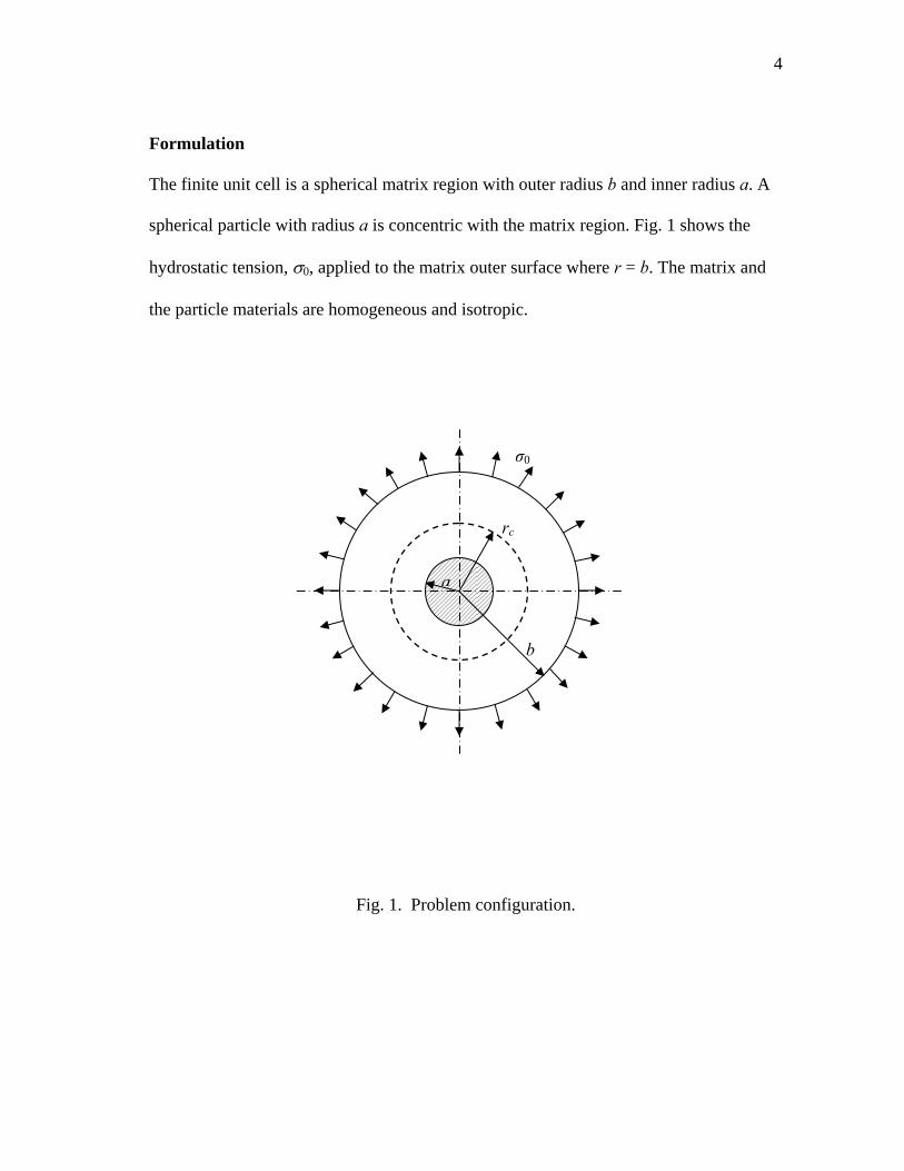
The finite unit cell is a spherical matrix region with outer radius b and inner radius a. A

spherical particle with radius a is concentric with the matrix region. Fig. 1 shows the

hydrostatic tension, σ0, applied to the matrix outer surface where r = b. The matrix and

the particle materials are homogeneous and isotropic.

b

rc

σ0

a

Fig. 1. Problem configuration.

5

The particle bonds perfectly to the elastic-plastic matrix with interface tension, pi, and

behaves elastically under σ0. A classical plasticity model (e.g., Wilner, 1988) uses the

same hydrostatic loading and a similar unit cell (with b → ∞).

The entire matrix remains elastic when σ0 is sufficiently small. When σ0 becomes large

enough the matrix yields from its inner surface because the hard particle induces a stress

concentration. The yielded region expands as σ0 continues to increase. From symmetry,

the elastic-plastic interface in the matrix is a spherical surface for any σ0 that produces a

plastic region.

The elasto-plastic radius is rc and the associated interface tension is pc. Thus, the matrix

material within a ≤ r ≤ rc is plastic and the material within rc ≤ r ≤ b remains elastic

under σ0.

Eqs. (3a,b) show the elastic power-law hardening material in a complex stress state (e.g.,

Gao, 1992, 2003).

⎪⎩

⎪⎨⎧

>

≤=

)(

)(

yene

yeeHe

E

σσκε

σσεσ (3a,b)

E is Young’s modulus, n (0 ≤ n ≤ 1) is the strain-hardening exponent, σy is the yield

stress, κ is a material constant satisfying κ = σy1−nEn. Eqs. (3a,b) recover the stress-strain

relation for elastic-perfectly plastic materials when n = 0. They reduce to Hooke’s law

for linearly elastic materials when n = 1.

6

This constitutive model describes the matrix material. Moreover, Eq. (3b) is the

homogeneous part of the effective stress, σeH, in the strain gradient plasticity theory in

Eq. (1) and Eq. (2). The solution in the plastic region uses this relationship. The material

response in the elastic region obeys Hooke’s law, Eq. (3a). This enables the direct

application of Lamé’s classical elasticity solution in the elastic region.

For infinitesimal deformations considered in the current formulation, the boundary

conditions at the perfectly bonded particle-matrix interface are

.andar

I

ar

M

ar

Irrar

Mrr uu

====== σσ (4a,b)

The superscripts M and I denote the matrix and inclusion, respectively. σrr is the radial

stress component and u is the only non-vanishing radial displacement component. Eqs.

(4a,b) ensure the traction and displacement continuities at the interface where r = a.

The elastic-plastic problem is now a boundary-value problem with an analytical solution.

Solution for the elastic inclusion (0 )r a≤ ≤

The inclusion is an elastic, solid sphere with radius a subjected to the uniform tension,

pi, normal to its surface. Lamé’s solution for a pressurized spherical shell (e.g.,

Timoshenko, 1970) gives the stress components as

,irr p=== φφθθ σσσ (5)

and the displacement component as

1 2 .I

iIuE

ν−= p r (6)

7

EI and vI denote the inclusion’s elastic modulus and Poisson’s ratio, respectively. pi is a

constant parameter, i.e., it depends on σ0 and material properties. Eq. (5) shows that the

inclusion is in a constant stress state.

Solution for the matrix in the elastic region ( )cr r b≤ ≤

This region is a thick-walled spherical shell with inner radius, rc, and outer radius, b. The

internal tension, pc, and external tension, σ0, act on the region. Lamé’s solution for a

pressurized spherical shell (e.g., Timoshenko, 1970) yields the stress components as

,2

12

1

,11

3

3

33

3

3

3

33

30

3

3

33

3

3

3

33

30

⎟⎟⎠

⎞⎜⎜⎝

⎛+

−−⎟⎟

⎠

⎞⎜⎜⎝

⎛+

−==

⎟⎟⎠

⎞⎜⎜⎝

⎛−

−+⎟⎟

⎠

⎞⎜⎜⎝

⎛−

−=

rb

rbrp

rr

rbbσ

σσ

rb

rbrp

rr

rbbσ

σ

c

ccc

cθθ

c

ccc

crr

φφ

(7)

and the displacement component as

.rb

rbrp

rr

rbbσ

νr

brb

rpr

rrb

bσν

Eru

c

ccc

cc

ccc

c ⎪⎭

⎪⎬⎫

⎥⎥⎦

⎤

⎢⎢⎣

⎡⎟⎟⎠

⎞⎜⎜⎝

⎛−

−+⎟⎟

⎠

⎞⎜⎜⎝

⎛−

−−

⎪⎩

⎪⎨⎧

⎥⎥⎦

⎤

⎢⎢⎣

⎡⎟⎟⎠

⎞⎜⎜⎝

⎛+

−−⎟⎟

⎠

⎞⎜⎜⎝

⎛+

−−= 11

21

21)1( 3

3

33

3

3

3

33

30

3

3

33

3

3

3

33

30

(8)

The solution in Eq. (7) and Eq. (8) contains two unknown parameters, pc and rc.

On the elastic-plastic interface where r = rc, the stress components in Eq. (7) must satisfy

the yield condition

.| yrre cσσ == (9)

This provides the first relation for determining cp and .cr

8

Solution for the matrix in the plastic region ( )ca r r≤ ≤

The governing equations below assume infinitesimal deformations, isotropic hardening,

incompressibility, and monotonic loading. These equations embody Hencky’s

deformation theory, strain gradient plasticity theory, and the elastic power-law hardening

model. The governing equations include the equilibrium equation,

;21

drd

r rrrr

σσσ θθ =− (10)

the compatibility equation,

;θθθθ εε

ε−= rrdr

dr (11)

and the constitutive equations,

1( ), ( )2

e err rr rr

e e

,θθ θθ θθ φφε εε σ σ ε σ σ εσ σ

= − − = − = (12)

,2e

nee c εκεσ ∇−= (13)

.e rθθ rσ σ σ= − (14)

The boundary conditions are

| , |crr r a i rr r r cp pσ σ= == = , (15a,b)

,|,|E

D yrreare c

σεε == == (16a,b)

where D is a constant. Eqs. (15a,b) are two standard boundary conditions in classical

plasticity. Eqs. (16a,b) are two extra boundary conditions arising from strain gradient

plasticity theory.

9

Eq. (10) to Eq. (16a,b) defines the boundary-value problem (BVP) determining the stress

and displacement components in the plastic region. The solution gives the stress

components as

,23

561

231

321

32

561

321

32

5

5

5

53

2

3

3

3

0

5

5

5

53

23

3

3

3

0

⎪⎭

⎪⎬⎫

⎪⎩

⎪⎨⎧

⎟⎟⎠

⎞⎜⎜⎝

⎛+⎟

⎠

⎞⎜⎝

⎛−⎥⎥⎦

⎤

⎢⎢⎣

⎡⎟⎠

⎞⎜⎝

⎛⎟⎠⎞

⎜⎝⎛ −++⎟

⎟⎠

⎞⎜⎜⎝

⎛−−==

⎥⎥⎦

⎤

⎢⎢⎣

⎡⎟⎟⎠

⎞⎜⎜⎝

⎛−⎟

⎠

⎞⎜⎝

⎛⎟⎟⎠

⎞⎜⎜⎝

⎛−⎟

⎟⎠

⎞⎜⎜⎝

⎛−+⎟

⎟⎠

⎞⎜⎜⎝

⎛−−=

ra

ra

ar

ac

Eσ

rrn

nσ

brσ

σσσ

,ra

ra

ar

Eσ

ac

rr

nσ

brσ

σσ

c

cyn

cycyθθ

c

cyn

ncycy

rr

φφ

(17)

and the displacement component as

2

3

21

rr

Eu cyσ

= . (18)

Eq. (19) defines rc as

⎥⎥⎦

⎤

⎢⎢⎣

⎡⎟⎟⎠

⎞⎜⎜⎝

⎛−⎟

⎠⎞

⎜⎝⎛

⎟⎟⎠

⎞⎜⎜⎝

⎛−⎟

⎟⎠

⎞⎜⎜⎝

⎛−⎟

⎠⎞

⎜⎝⎛−

⎟⎟⎠

⎞⎜⎜⎝

⎛−−=⎟

⎠⎞

⎜⎝⎛

−

5

53

23

33

3

3

0

3

1561

32

13

2212

1

c

cyn

c

nncy

cycyI

I

ra

ar

Eσ

ac

ra

ar

nσ

brσ

σar

Eσ

νE

(19)

for given values σ0, E, σy, n, c, EI, vI, a and b. The remaining three parameters are

.,13

2,

2121

3

3

3

33

ar

ED

br

par

Eσ

νEp cycy

occy

I

I

i

σσσ =⎟

⎟⎠

⎞⎜⎜⎝

⎛−−=⎟

⎠⎞

⎜⎝⎛

−= (20a–c)

The stress and displacement components for the inclusion now come from Eq. (5) and

Eq. (6). Eq. (7) and Eq. (8) give the components in the elastic region.

10

CHAPTER 3

SPECIFIC SOLUTIONS

Classical plasticity solution

Eq. (10) to Eq. (16a,b) defines the BVP in the plastic region. These equations reduce to

formulas from Hencky deformation theory and the von Mises yield criterion when c = 0.

Hence, letting c = 0 in Eq. (17) gives the stress components.

⎥⎥⎦

⎤

⎢⎢⎣

⎡⎟⎠

⎞⎜⎝

⎛⎟⎠⎞

⎜⎝⎛ −++⎟

⎟⎠

⎞⎜⎜⎝

⎛−−==

⎟⎟⎠

⎞⎜⎜⎝

⎛−+⎟

⎟⎠

⎞⎜⎜⎝

⎛−−=

ncycy

o

n

ncycy

orr

rrn

nbr

rr

nbr

3

3

3

3

3

3

3

12

313

21

32

13

21

32

σσσσσ

σσσσ

φφθθ

(21)

Eq. (19) reduces to Eq. (22) and gives rc.

⎟⎟⎠

⎞⎜⎜⎝

⎛−⎟

⎠

⎞⎜⎝

⎛−⎟⎟⎠

⎞⎜⎜⎝

⎛−−=⎟

⎠

⎞⎜⎝

⎛− n

c

nncycy

ocy

I

I

ra

ar

nbr

ar

EE

3

33

3

33

13

21

32

2121 σσ

σσ

ν (22)

Inclusion in an infinitely large elastic-plastic matrix

The elastic-plastic matrix becomes infinitely large as b approaches infinity. Letting

b → ∞ in Eq. (17) gives the stress components.

⎪⎭

⎪⎬⎫

⎪⎩

⎪⎨⎧

⎟⎟⎠

⎞⎜⎜⎝

⎛+⎟

⎠

⎞⎜⎝

⎛−⎥⎥⎦

⎤

⎢⎢⎣

⎡⎟⎠

⎞⎜⎝

⎛⎟⎠⎞

⎜⎝⎛ −++−==

⎥⎥⎦

⎤

⎢⎢⎣

⎡⎟⎟⎠

⎞⎜⎜⎝

⎛−⎟

⎠

⎞⎜⎝

⎛⎟⎟⎠

⎞⎜⎜⎝

⎛−⎟

⎟⎠

⎞⎜⎜⎝

⎛−+−=

5

5

5

53

2

3

0

5

5

5

53

23

3

0

23

561

231

32

32

561

32

32

ra

ra

ar

ac

Eσ

rrn

nσσ

σσσ

ra

ra

ar

Eσ

ac

rr

nσσ

σσ

c

cyn

cyyθθ

c

cyn

ncyy

rr

φφ

(23)

Solving Eq. (24) gives rc.

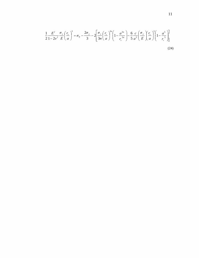
11

⎥⎥⎦

⎤

⎢⎢⎣

⎡⎟⎟⎠

⎞⎜⎜⎝

⎛−⎟

⎠

⎞⎜⎝

⎛⎟⎟⎠

⎞⎜⎜⎝

⎛−⎟

⎟⎠

⎞⎜⎜⎝

⎛−⎟

⎠

⎞⎜⎝

⎛−−=⎟⎠

⎞⎜⎝

⎛− 5

53

23

33

0

3

1561

32

32

2121

c

cyn

c

nncyycy

I

I

ra

ar

Eσ

ac

ra

ar

nσσ

σar

Eσ

νE

(24)

12

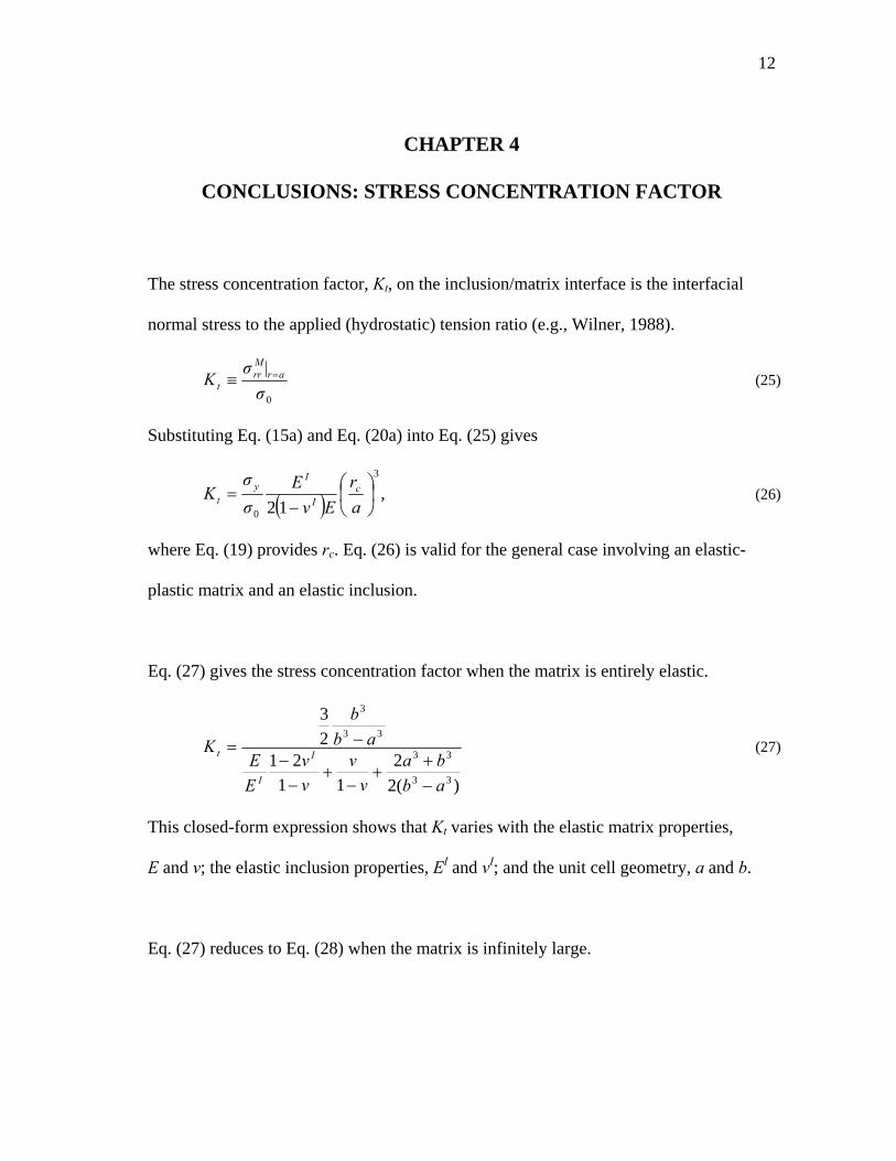
CHAPTER 4

CONCLUSIONS: STRESS CONCENTRATION FACTOR

The stress concentration factor, Kt, on the inclusion/matrix interface is the interfacial

normal stress to the applied (hydrostatic) tension ratio (e.g., Wilner, 1988).

0σ|σ

K arMrr

t=≡ (25)

Substituting Eq. (15a) and Eq. (20a) into Eq. (25) gives

( ) ,12

3

0

⎟⎠⎞

⎜⎝⎛

−=

ar

EνE

σσ

K cI

Iy

t (26)

where Eq. (19) provides rc. Eq. (26) is valid for the general case involving an elastic-

plastic matrix and an elastic inclusion.

Eq. (27) gives the stress concentration factor when the matrix is entirely elastic.

)(22

1121

23

33

33

33

3

abba

νν

νν

EE

abb

K I

I

t

−+

+−

+−

−−= (27)

This closed-form expression shows that Kt varies with the elastic matrix properties,

E and v; the elastic inclusion properties, EI and vI; and the unit cell geometry, a and b.

Eq. (27) reduces to Eq. (28) when the matrix is infinitely large.

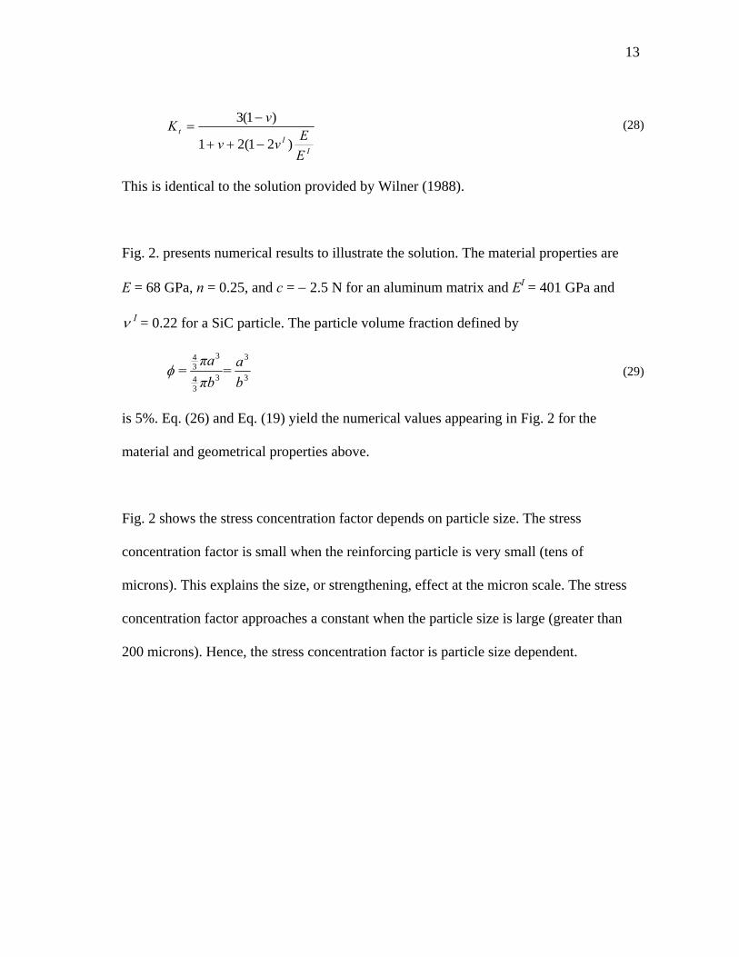
13

II

t

EEνν

νK)21(21

)1(3

−++

−= (28)

This is identical to the solution provided by Wilner (1988).

Fig. 2. presents numerical results to illustrate the solution. The material properties are

E = 68 GPa, n = 0.25, and c = − 2.5 N for an aluminum matrix and EI = 401 GPa and

ν I = 0.22 for a SiC particle. The particle volume fraction defined by

3

3

334

334

ba=

πbπa

=φ (29)

is 5%. Eq. (26) and Eq. (19) yield the numerical values appearing in Fig. 2 for the

material and geometrical properties above.

Fig. 2 shows the stress concentration factor depends on particle size. The stress

concentration factor is small when the reinforcing particle is very small (tens of

microns). This explains the size, or strengthening, effect at the micron scale. The stress

concentration factor approaches a constant when the particle size is large (greater than

200 microns). Hence, the stress concentration factor is particle size dependent.

14

0

1

2

3

4

5

6

0.00 0.10 0.20 0.30 0.40 0.50

a (mm)

Kt

φ = 5%r c /a = 2

Fig. 2. Stress concentration factor as a function of the inclusion size.

15

REFERENCES

Chawla, N., Shen, Y.-L., 2001. Mechanical behavior of particle reinforced metal matrix composites. Adv. Eng. Mater. 3, 357-370.

Gao, X.-L., 1992. An exact elasto plastic solution for an open ended thick walled

cylinder of a strain-hardening material. Int. J. Pres. Ves. Piping 52, 129-144. Gao, X.-L, 2003. Elasto-plastic analysis of an internally pressurized thick-walled

cylinder using a strain gradient plasticity theory. Int. J. Solids Struct. 40, 6445-6455. Hutchinson, J.W., 2000. Plasticity at the micron scale. Int. J. Solids Struct. 37, 225-238. Lloyd, D.J., 1994. Particle reinforced aluminum and magnesium matrix composites. Int.

Mater. Rev. 39, 1-23. Miracle, D.B., 2005. Metal matrix composites – from science to technological

significance. Compos. Sci. Tech. 65, 2526-2540. Mühlhaus, H.-B., Aifantis, E.C., 1991. A variational principle for gradient plasticity. Int.

J. Solids Struct. 28, 845-857. Timoshenko, S.P., Goodier, J.N., 1970. Theory of Elasticity, 3rd ed. McGraw Hill, New

York. Wilner, B., 1988. Stress analysis of particles in metals. ASME J. Appl. Mech. 55, 355-

360.

16

CONTACT INFORMATION

Name: Matthew Wade Harris Address: Department of Mechanical Engineering, Texas A&M University,

3123 TAMU, College Station, TX 77843 Email Address: m_harris@tamu.edu Education: B.S. Mechanical Engineering. Texas A&M University. Expected

graduation, May 2008.