Icarus 222 (2013) 243–253

Contents lists available at SciVerse ScienceDirect

Icarus

journal homepage: www.elsevier .com/locate / icarus

A new approach to determining asteroid masses from planetaryrange measurements

Petr Kuchynka ⇑, William M. FolknerJet Propulsion Laboratory, California Institute of Technology, Pasadena, CA 91109, United States

a r t i c l e i n f o

Article history:Received 16 August 2012Revised 27 October 2012Accepted 6 November 2012Available online 14 November 2012

Keywords:AsteroidsPlanetary dynamicsCelestial mechanics

0019-1035/$ - see front matter � 2012 Elsevier Inc. Ahttp://dx.doi.org/10.1016/j.icarus.2012.11.003

⇑ Corresponding author.E-mail address: petr.kuchynka@jpl.nasa.gov (P. Ku

a b s t r a c t

We describe a new approach to estimate asteroid masses from planetary range measurements. Theapproach significantly simplifies the process of parameter estimation and allows an effective control ofsystematic errors introduced by the omission of asteroids from the dynamical model. All asteroid massesare adjusted individually thus avoiding the usual distinction between masses considered individually andmasses based on densities within the C, S and M taxonomic classes. Regularization is achieved byaccounting, on each mass, for a prior uncertainty determined from available estimations of asteroiddiameters and densities.

The new approach is used to fit the asteroid model of the JPL planetary ephemeris to Mars range data.The adjusted planetary solutions exhibit similar extrapolation capacity as previous releases of the JPLephemeris. Up to 27 asteroid masses are determined to better than 35%. The masses agree well with esti-mates obtained independently by other authors. The determined masses are also robust with respect tocross-validation on a dataset with a shorter time-span and with respect to a different selection of aster-oids in the model.

� 2012 Elsevier Inc. All rights reserved.

1. Introduction

Since the advent of space exploration, the tracking of planetarymissions provides measurements of distances between the Earthand the other planets. The high accuracy of the measurements al-lows the detection of asteroid perturbations induced on the plan-ets, making then possible the determination of asteroid masses.Mars range is especially sensitive to the perturbations, because ofthe planet’s proximity with the asteroid belt. Standish and Hellings(1989) were the first to determine asteroid masses from rangedata. Based on the tracking of the Viking landers, the authors esti-mated the masses of 1 Ceres, 2 Pallas and 4 Vesta. The procedurerequired a complete dynamical model of the Solar System, ableto accurately predict the evolution of the planets. Asteroid masseswere then determined by adjusting the parameters of the model,including the asteroid masses, in order to match the model predic-tions to the range observations. The procedure is closely related tothe construction of modern planetary ephemerides (e.g. Folkneret al., 2009).

Today, range measurements are available from a variety of mis-sions. In particular, since 1999 the distance to Mars is measured al-most continuously with an accuracy of about 1 m. This allows theestimation of a relatively large number of asteroid masses.

ll rights reserved.

chynka).

Recently, Konopliv et al. (2011) estimated 21 masses. Using lessconservative uncertainties, Fienga et al. (2009) estimated up to33 masses. For comparison, the total number of asteroid massesobtained so far by other methods is about 100 (Carry, 2012). Suchestimations rely on astrometric observations of close encountersbetween asteroids, on observations of asteroid satellites or, in afew cases, on spacecraft encounters with asteroids.

As more planetary range measurements become available, boththe number of constraints on asteroid masses and the challenge toproperly estimate these constraints steadily grow. It is then essen-tial to establish an effective methodology for parameter estimationand error control in order to guarantee the reliability of the esti-mated asteroid masses.

1.1. A challenging inverse problem

The determination of asteroid masses from range observationsinvolves two steps: selection and regularization. The selection stepconsists in determining the asteroids to include in the dynamicalmodel, that is, the asteroids with a significant effect on the rangedata. As discussed in Williams (1984), the selection should bebased on both the amplitudes and the frequencies of the asteroidperturbations. It should also account for free parameters in thedynamical model, such as the initial states of the planets, thatcan absorb the asteroid effects. Regardless of the exact criteria usedto compare asteroid perturbations, selections usually contain

244 P. Kuchynka, W.M. Folkner / Icarus 222 (2013) 243–253

about 300 asteroids. Recent releases of the JPL planetary ephem-eris, e.g. DE421 (Folkner et al., 2009), include 343 asteroids deter-mined by analytical considerations similar to Williams (1984). Asthe asteroid perturbations are proportional to asteroid masses,the amplitudes of the perturbations are poorly constrained andany recommended selection is necessarily tentative. The regulari-zation step is required in order to reduce the correlations betweenthe asteroid perturbations to a level where individual asteroidmasses can be estimated. This is achieved by combining the rangedata with some additional information. The standard approach toregularization was introduced by Hellings et al. (1983) (see alsoWilliams, 1984). Asteroids in the dynamical model are split intoobjects with masses adjusted individually and objects grouped intothree taxonomic classes (C, S and M). Within each class, objects areassumed to have a common density. Asteroid masses are thendetermined by adjusting the class density and using a diameterestimated for example from radiometric observations. In the fol-lowing, the regularization introduced by Hellings et al. (1983) willbe referred to as the standard approach. The C and S classes used inthe regularization correspond in practice to the C and S complexesof modern taxonomic classifications and comprise several individ-ual taxonomic classes (Bus et al., 2002). In this paper, we use theterms class and complex interchangeably.

Both the selection and regularization steps introduce system-atic errors in the estimated parameters. As it is impossible to in-clude in the dynamical model all asteroids, systematic errorsfrom selection are unavoidable. Systematic errors from regulariza-tion are due to any imperfect or arbitrary aspect of the regulariza-tion. In the standard approach for example, systematic errors areon one hand introduced by the necessarily imperfect selectionincluding only about 300 asteroids and, on the other hand, byimperfect asteroid diameters and the assumption of constant den-sities within the taxonomic classes.

1.2. Estimations using the standard approach

Since Standish and Hellings (1989), many different authors haveestimated asteroid masses from range data. The estimates are oftenprovided as by products of a planetary ephemeris release. Asteroidmasses recently obtained using the JPL ephemeris are available inKonopliv et al. (2006, 2011). Masses are also regularly reported inthe French ephemeris INPOP (e.g. Fienga et al., 2008, 2009) and inthe Russian ephemeris EPM (e.g. Pitjeva, 2005, 2010).

All determinations prior to and including Konopliv et al. (2011)use the standard approach, defined in the previous section, or someof its variants. The variants include the estimation of individualmasses using prior uncertainties or the fixing of some masses tovalues determined independently of planetary range (Konoplivet al., 2006; Fienga et al., 2009; Somenzi et al., 2010). In order toreduce correlations between asteroid perturbations, Somenziet al. (2010) suggest to adjust asteroid masses using only shorttime intervals where the amplitudes of the perturbations are par-ticularly favorable. Another improvement to the standard ap-proach is the implementation in the dynamical model of a solidring centered at the Sun and extending to about 2.8 au. The ring

Table 1A selection of estimated masses of 4 Vesta published prior to Konopliv et al. (2011). The lExcept for Konopliv et al. (2006), Pitjeva (2010), and Konopliv et al. (2011), the uncertaintiesto noise in observations. The masses are provided as GM (km3 s�2).

Pitjeva (2005) Konopliv et al. (2006) Fienga et al. (2008) Fienga

17.84 18.02 17.76 18.47±0.01 ±0.21 ±0.03 ±0.20

a Russell et al. (2012).

is intended to represent the large number of weakly perturbingasteroids omitted from the model (Williams, 1984; Krasinskyet al., 2002; Kuchynka et al., 2010).

Determinations based on the standard approach share twodrawbacks. One drawback is the difficulty in estimating the sys-tematic errors in the adjusted masses, mainly introduced by theselection and regularization steps. The difficulty is apparent whencomparing various estimations of the mass of 4 Vesta, based onrange measurements, with the mass recently obtained from thetracking of the DAWN spacecraft (Table 1). In four out of the sixcases presented in Table 1, the difference between the mass ob-tained by DAWN and the estimate based on range amounts to sev-eral times the published uncertainty of the estimate. Systematicerrors are often ignored or estimated empirically. The empiricalestimation may consist in experimenting with different weightson observations and different sets of adjusted parameters (e.g.Pitjeva, 2010). It may also simply consist in multiplying formaluncertainties by a constant factor (e.g. Konopliv et al., 2006).Significant progress has been achieved by the introduction of con-sider covariance analysis. In Konopliv et al. (2011), the method isused to properly account for errors introduced by asteroid massesfixed to constant (non-adjusted) values. The second drawback ofthe standard approach is the difficulty in determining the list ofasteroid masses to adjust individually, as opposed to asteroidmasses estimated from diameters and taxonomic densities. Inprinciple, the list should be optimized to minimize systematicand random errors. Because of the difficulty of estimating system-atic errors, the list is optimized empirically according to some indi-rect criterion. For example in Folkner et al. (2009), the list isadapted in order to obtain a stable extrapolation of the dynamicalmodel. The list could also be fine tuned to adjust masses to realisticand stable values.

As a result of the previous drawbacks and the recourse to exper-imentation, the estimation of asteroid masses based on the stan-dard approach is imperfect and somewhat tedious.

1.3. Towards a new approach

An alternative to the standard approach is proposed in Kuchyn-ka (2010). It consists of adjusting all asteroid masses individuallyand achieving regularization by accounting for prior uncertainties.The uncertainties are based on available determinations of asteroiddiameters and densities. By considering all asteroids individually,we avoid the drawbacks of the standard approach. It is not neces-sary to determine a list of asteroids to adjust individually and theestimation of systematic errors is simplified. The process avoids re-course to experimentation and is thus easily adaptable to newobservations.

The new approach has been used to adjust the recent INPOP10planetary ephemeris (Fienga et al., 2011; Verma et al., 2012). Inthis paper, we apply the approach to estimating asteroid masseswith the JPL ephemeris. We provide a detailed description of theregularization and focus our interest specifically on the estimationof asteroid masses.

ast column contains the mass determined from the tracking of the DAWN spacecraft.of the estimates correspond to formal uncertainties reflecting only random errors due

et al. (2009) Pitjeva (2010) Konopliv et al. (2011) DAWNa

17.52 17.38 17.28814±0.40 ±0.27 ±0.00007

P. Kuchynka, W.M. Folkner / Icarus 222 (2013) 243–253 245

2. Theory

2.1. Least squares

It is useful to recall some properties of the least squares param-eter estimation. In the following, we assume a linear dependencybetween model parameters and observations. The dependencycan be achieved locally by linearizing the model around a set ofnominal parameter values. We use E(�) and Cov(�) to denote expec-tation and covariance.

Let us consider n measurements ~z ¼ ð~z1; . . . ;~znÞ of an observa-ble, such as planetary range, and a model with p parameters. Wethen have

~z ¼ eMbþ ~e; ð1Þ

where eM is a partials matrix, b = (b1, . . . , bp) is a vector of parame-ters and ~e ¼ ð~e1; . . . ; ~enÞ represents measurement noise. For anynon-singular square matrix W, the previous relation is strictlyequivalent to

W~z ¼W eMbþW~e: ð2Þ

In order to be efficient, the least squares method requires choosingW such that W2 ¼ Covð~eÞ�1. Matrix W2 is usually referred to as theweight matrix. For uncorrelated noise, the matrix is diagonal witheach diagonal component equal to the inverse of the variance ofthe corresponding component in ~e. We define z ¼W~z;M ¼W eM;

e ¼W~e and rewrite (2) as

z ¼ Mbþ e: ð3Þ

Assuming that b contains some unknown values, the least squaresestimates of these values, denoted b = (b1, . . . , bp), are given by

b ¼ ðMT MÞ�1MT z: ð4Þ

The recovery of b is conditioned upon M being full rank and n P p.Injecting (3) into (4), we obtain

b ¼ bþ ðMT MÞ�1MTe: ð5Þ

In the absence of noise, the recovery is perfect (b = b). In the pres-ence of noise, each component ~e may be considered as an indepen-dent random variable with zero expectation. The components of eand b are then also random variables depending linearly on ~e. Forany matrix A and a random variable vector X, the covariance of a lin-early dependent variable Y = AX is given by (e.g. Bickel and Doksum,2001)

CovðYÞ ¼ A CovðXÞAT: ð6Þ

With Eq. (6), we verify that Cov(e) is an identity matrix. Using (6)and (5), as well as classic properties of expectations, we then obtain

EðbÞ ¼ b; CovðbÞ ¼ ðMT MÞ�1: ð7Þ

Least squares estimates provided by (4) are thus unbiased and theiruncertainties are given by the above expression of Cov(b).

2.2. Prior uncertainties

Accounting for prior uncertainties in an adjustment is equiva-lent to relying on additional information independent of the mea-surements. Lets consider information available as unbiased andindependent estimates l = (l1, . . . , lp) of the model parametersb. The prior uncertainties on the parameters are given by Cov(l).We thus have

l ¼ bþ Ce0; ð8Þ

where C is a diagonal square matrix such that C2 = Cov(l) ande0 ¼ e01; . . . ; e0p

� �is a vector of random variables with zero

expectation and variance equal to one. Treating the estimates l asobservations and combining with z, we obtain

z

C�1l

� �¼

M

C�1

� �bþ

ee0

� �: ð9Þ

In the above equation, the matrix C�1 ensures that the observationsare properly weighted. The least square estimates of the modelparameters based on the combined set of observations are

b ¼ C�1ðMT zþ C�2lÞ; ð10Þwhere C ¼ MT M þ C�2:

Injecting Eqs. (3) and (8) into (10) leads to

b ¼ bþ C�1 M

C�1

� �T ee0

� �: ð11Þ

Using this expression with the covariance relation (6) and proper-ties of expectations, we obtain

EðbÞ ¼ b; CovðbÞ ¼ C�1: ð12Þ

Note that setting C�1 to zero is equivalent to considering the casewithout any prior constraints.

The least squares estimate (10) minimizes the Euclidean norm

z

C�1l

� ��

M

C�1

� �b

��������

2

2

¼ kz�Mbk22 þ kC

�1ðl� bÞk22: ð13Þ

The use of prior uncertainties is thus equivalent to Tikhonovregularization (Hansen, 1977). Parameters are estimated so as tomaintain the model prediction close to the observations and simul-taneously maintain the parameters close to the prior estimates l.As opposed to the standard approach to regularization defined insubsection 1.1, we will refer to the regularization provided by(10) as Tikhonov regularization. Uncertainties of the estimates ob-tained with the Tikhonov approach, given by the expression ofCov(b) in (12), will be referred to as posterior uncertainties.

2.3. Systematic errors from omitted asteroids

Tikhonov regularization does not introduce systematic errors solong as the prior estimates l are unbiased. Nevertheless, system-atic errors will occur if the adjusted model does not contain allthe parameters acting on the observations. We denote by bg andMg the vector of parameters and the partials matrix correspondingto asteroid masses not accounted in the dynamical model. Insteadof (3), the range measurements are then expressed as

z ¼ MbþMgbg þ e: ð14Þ

Let lg be some prior estimate of the omitted masses. By analogywith (8), we have

lg ¼ bg þ Cge0g ; ð15Þ

where C2g ¼ CovðlgÞ and e0g is a vector of random variables with zero

expectation and variance equal to one. By injecting (14) into theTikhonov regularization formula (10), we obtain

b ¼ bþ br þ bs;

where br ¼ C�1 M

C�1

� �T ee0

� �bs ¼ C�1MT Mgbg :

ð16Þ

We call br and bs respectively the random and systematic errors.Note that br corresponds to the errors considered in subsection2.2. The expectations and covariances of br and bs are given by

246 P. Kuchynka, W.M. Folkner / Icarus 222 (2013) 243–253

EðbrÞ ¼ 0CovðbrÞ ¼ C�1

EðbsÞ ¼ C�1MT Mglg

CovðbsÞ ¼ C�1MT MgC2g MT

g MC�T :

ð17Þ

Assuming that e, e0 and e0g are independent, we have

EðbÞ ¼ bþ EðbsÞ; CovðbÞ ¼ CovðbrÞ þ CovðbsÞ: ð18Þ

The above expressions allow the estimation of realistic uncertain-ties accounting for both random errors introduced by noise and sys-tematic errors introduced by selection. The estimation of systematicerrors relies on prior knowledge of the asteroid masses omitted inthe model. Without such knowledge, the systematic errors are en-tirely undetermined. Omitting asteroids from the model is equiva-lent to keeping the asteroids in the model with masses held fixedand equal to zero. If instead of fixing non-adjusted asteroid massesto zero, we fix them to lg, Eqs. (17) and (18) still apply, except thatthe expectations of the systematic errors drop to zero. Albeit differ-ent notations, the expression for the covariance of bs in (17) corre-sponds to the standard consider covariance derived in Bierman(1977) and used in Konopliv et al. (2011) to account for systematicerrors from asteroids with fixed masses.

3. Constraints on asteroid masses

3.1. Initial selection

The number of cataloged asteroids amounts today to severalhundreds of thousands. It is impractical, if not impossible, to con-sider all of them. We thus restrict our study to a selection of 3714objects. The selection corresponds to numbered asteroids in theMinor Planet Center orbit database (MPCORB1) with absolute mag-nitudes lower than 12 and primary designations lower than 219,017.The cut-off in absolute magnitude eliminates asteroids with diame-ters smaller than about 20 km. Beside a majority of main-belt aster-oids, the selection includes approximately 200 trans-Neptunianobjects (TNOs).

3.2. Prior masses

For each of the 3714 asteroids, we need to determine a priorestimate of mass and a prior uncertainty. As the size of the selec-tion exceeds by far the number of currently determined masses,the prior estimates will be based on available determinations ofasteroid diameters.

Over 100,000 diameters have been determined from WISE in-fra-red observations (Masiero et al., 2011). The principle of esti-mating asteroid size from thermal emission is described in Harrisand Lagerros (2002). Combining the WISE data with diametersbased on earlier infra-red surveys, SIMPS and MIMPS (Tedescoet al., 2004a,b), size estimates are available for more than 2000out of the 3714 asteroids in the selection. For each of these objects,we compute a nominal diameter and a corresponding uncertainty.The data from the three surveys is combined assuming normal dis-tributions of errors with standard deviations given by the uncer-tainties of the various diameter estimates. Uncertainties of WISEdiameters are taken equal to the formal uncertainties providedwith the data. SIMPS and MIMPS diameters smaller than 40 kmare considered as unreliable and they are ignored. Diameters largerthan 100 km have an estimated accuracy of 10% (Tedesco et al.,2002). Below 100 km, we assume a linear degradation of accuracywith size, down to 35% for diameters of 40 km.

1 The database is available at http://www.minorplanetcenter.net.

In three cases, significant differences exist between the com-puted nominal diameters and estimates published independentlyof any of the three surveys. For these asteroids, the independentestimates are used to replace the computed diameters and uncer-tainties. Thus for 16 Psyche, the nominal diameter is set to186 ± 30 km (Shepard et al., 2008), for 65 Cybele to 273 ± 12 km(Müller and Blommaert, 2004), and for 90 Antiope to 108 ± 1 km(Descamps et al., 2007, based on the size of both binary compo-nents). We use the estimates available in Stansberry et al. (2008)to update the nominal diameters of several TNOs in the selection.

For asteroids where no estimate of size is available or where thesize uncertainty is larger than 35%, the nominal diameter is com-puted assuming an albedo of 0.1 and (Harris and Lagerros, 2002)

D ðkmÞ ¼ 1329ffiffiffiffiqp 10�0:2H; ð19Þ

where H represents absolute magnitude, q the albedo, and D thediameter. At this point all of the 3714 asteroids have a nominaldiameter. We assign to each object a prior mass computed assum-ing a spherical shape and a density of 2.2 g cm�3.

3.3. Prior uncertainties

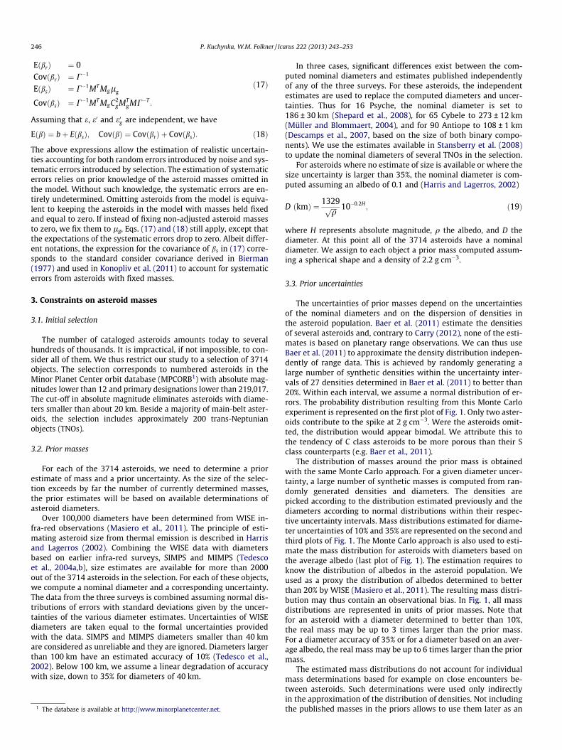
The uncertainties of prior masses depend on the uncertaintiesof the nominal diameters and on the dispersion of densities inthe asteroid population. Baer et al. (2011) estimate the densitiesof several asteroids and, contrary to Carry (2012), none of the esti-mates is based on planetary range observations. We can thus useBaer et al. (2011) to approximate the density distribution indepen-dently of range data. This is achieved by randomly generating alarge number of synthetic densities within the uncertainty inter-vals of 27 densities determined in Baer et al. (2011) to better than20%. Within each interval, we assume a normal distribution of er-rors. The probability distribution resulting from this Monte Carloexperiment is represented on the first plot of Fig. 1. Only two aster-oids contribute to the spike at 2 g cm�3. Were the asteroids omit-ted, the distribution would appear bimodal. We attribute this tothe tendency of C class asteroids to be more porous than their Sclass counterparts (e.g. Baer et al., 2011).

The distribution of masses around the prior mass is obtainedwith the same Monte Carlo approach. For a given diameter uncer-tainty, a large number of synthetic masses is computed from ran-domly generated densities and diameters. The densities arepicked according to the distribution estimated previously and thediameters according to normal distributions within their respec-tive uncertainty intervals. Mass distributions estimated for diame-ter uncertainties of 10% and 35% are represented on the second andthird plots of Fig. 1. The Monte Carlo approach is also used to esti-mate the mass distribution for asteroids with diameters based onthe average albedo (last plot of Fig. 1). The estimation requires toknow the distribution of albedos in the asteroid population. Weused as a proxy the distribution of albedos determined to betterthan 20% by WISE (Masiero et al., 2011). The resulting mass distri-bution may thus contain an observational bias. In Fig. 1, all massdistributions are represented in units of prior masses. Note thatfor an asteroid with a diameter determined to better than 10%,the real mass may be up to 3 times larger than the prior mass.For a diameter accuracy of 35% or for a diameter based on an aver-age albedo, the real mass may be up to 6 times larger than the priormass.

The estimated mass distributions do not account for individualmass determinations based for example on close encounters be-tween asteroids. Such determinations were used only indirectlyin the approximation of the distribution of densities. Not includingthe published masses in the priors allows to use them later as an

0.0

0.2

0.4

0.6

0.8

1.0

[ g cm−3 ]

prob

abilit

y di

strib

utio

n (a)

0.0

0.2

0.4

0.6

0.8

1.0

[ units of prior mass ]

(b)

0.0

0.2

0.4

0.6

0.8

1.0

[ units of prior mass ]

(c)

0 1 2 3 4 5 −1 0 1 2 3 4 5 6 −1 0 1 2 3 4 5 6 −1 0 1 2 3 4 5 60.0

0.2

0.4

0.6

0.8

1.0

[ units of prior mass ]

(d)

Fig. 1. (a) Probability distribution of asteroid densities based on estimates in Baer et al. (2011). (b) Probability distribution of asteroid masses for objects with diametersknown to better than 10%. (c) Idem as (b), but for diameter uncertainties of 35%. (d) Idem as (b), but for asteroids without an accurate diameter estimate. In plots (b)-(d), asolid line represents the normal approximation defined for each mass distribution in Section 3.4.

P. Kuchynka, W.M. Folkner / Icarus 222 (2013) 243–253 247

independent check of the reliability of masses adjusted from rangemeasurements.

3.4. Normal approximations

For asteroids with poorly determined diameters, the mass dis-tributions are strongly skewed. It is difficult to predict how theseskewed distributions combine into the posterior uncertainties.The formulas derived in Section 2.2 provide the expectationsand variances of the posterior error distributions, but they havelittle utility if the shapes of the distributions are uncertain. In or-der to avoid this inconvenience, we replace the prior mass distri-butions with normal approximations. Assuming that noise in therange measurements is normally distributed, the approximationhas the advantage that all random variables involved in the equa-tions of Section 2.2 become normally distributed. In particular, thedistributions of errors in the adjusted parameters become normal.The expectations and variances provided by (12) have then simplegeometric interpretations. Using the approximations instead ofthe original mass distributions has the disadvantage of introduc-ing systematic errors in the regularization. At the cost of loosingsome constraints from the prior information, we may mitigatethe effect by choosing the approximating distributions sufficientlylarge.

We denote by Nðl;rÞ a normal distribution centered at l andwith standard deviation r. Both l and r are expressed in units ofprior masses. We approximate the mass distributions for asteroidswith diameter uncertainties of 10% and 35% by Nð1;0:53Þ andNð1;1:7Þ respectively. For asteroids with diameters based on anaverage albedo of 0.1, we use Nð1;2Þ. In each case, the value ofr guarantees that at least 68% and 95% of the prior distributionare contained respectively within ±r and ±2r of the approxima-tion. The three approximations are represented on Fig. 1. A linearinterpolation of r between the values of 0.53 and 1.7 is used toapproximate the mass distributions for diameter uncertainties be-tween 10% and 35% (for uncertainties smaller than 10%, we useindiscriminately r = 0.53). We define, for each asteroid, the prioruncertainty on mass as the standard deviation of the correspond-ing normal approximation.

4. Observations and model parameters

Planetary observations considered in this paper are Mars rangemeasurements provided by the tracking of the two Viking landers(VIK), Mars Global Surveyor (MGS), Mars Odyssey (ODY) and MarsReconnaissance Orbiter (MRO). In terms of Mars range data, thedataset is thus similar to the dataset used in Konopliv et al.(2011). Range measurements are round-trip light-times of a range

signal between the Deep Space Network (DSN) and the landers orspacecraft. As discussed in Kuchynka et al. (2012), the measure-ments are preprocessed and calibrated for several effects, such asthe variations in round-trip light-times induced by the orbit ofthe spacecraft around Mars. The measurements are also binned,so each data point corresponds to observations averaged overone tracking pass. In order to mitigate the effect of the solar plasmadelay, we discard observations for Sun–Earth–Probe (SEP) angleslower than 15�. A small portion of the data, about 10%, is also dis-carded to reduce station specific calibration effects.

The range measurements will be used to adjust asteroid massesin a dynamical model similar to the one used for DE421 (Folkneret al., 2009). The model contains 343 asteroids and accounts forthe mutual perturbations of the Sun, the planets and the Moon ina parametrized post-Newtonian metric. Perturbations from theasteroids are accounted in an iterative manner. First, the asteroidorbits are integrated while accounting for mutual interactions,but holding the orbits of the Sun, the Moon and the planets fixedto positions in DE421. The orbits of the planets are then integratedwhile holding the asteroids fixed to positions determined in theprevious run. These numerical integrations span about 35 years:the time interval between today and the first Viking range mea-surements. Planetary integrations rely on the variable order Adamsmethod routinely used to integrate the JPL planetary ephemeris.Asteroids are integrated using a Gauss–Jackson method (Jackson,1924; Fox, 1984).

Mars range is insensitive to a large number of parameters in thedynamical model. Parameters adjusted in the Tikhonov regulariza-tion will thus include only the masses of the asteroids and the statevectors of Mars and the Earth–Moon barycentre at a referenceepoch. A scaling factor in the model of the solar plasma delay isalso adjusted. In this paper, we treat asteroid state vectors as per-fectly known. In practice, the asteroid states may involve uncer-tainties on the order of the arc second. Such variations inasteroid orbits have nevertheless very little impact on Mars range.In order to account for spacecraft transponder delays and stationspecific calibration effects, we adjust one bias for each spacecraftand each DSN station involved in acquiring the range data. Stationcalibration imperfections are revealed by comparing data from dif-ferent spacecraft over a common time span (see Kuchynka et al.,2012). As the majority of Viking data is available from only onelander, the detection of station calibration effects is impossible.In consequence, for Viking, we neglect potential station effects. Abias is nevertheless adjusted for each lander in order to accountfor transponder delays.

Tikhonov regularization relies on the partial derivatives of theobservations with respect to the adjusted model parameters. Wecompute all the partials by finite differences. A reference ephem-eris is obtained using zero asteroid masses. Model parameters

248 P. Kuchynka, W.M. Folkner / Icarus 222 (2013) 243–253

are then modified in order to compute the various partials. Settingasteroid masses to zero in the reference integration allows thecomputation of each partial by integrating at most one asteroidat a time. Neglecting second order asteroid perturbations in thepartials introduces small nonlinear terms in the dependency be-tween model predictions and model parameters. Nevertheless,these terms may be accounted for by iterating the parameter esti-mation process.

5. Results

In the previous sections, we determined the partials of observa-tions with respect to each of the model parameters and we alsodetermined the prior uncertainties on each asteroid mass. In con-sequence, at this point, we may apply the Tikhonov regularizationto actually estimate asteroid masses.

5.1. Additional asteroid selection

Numerically integrating 3714 interacting asteroids is computa-tionally demanding. The estimation of as many asteroid masses isrelatively demanding as well. Thus if we reduce the number ofasteroids in the model without introducing significant systematicerrors, we avoid heavy numerical computations and potential ef-fects from round off errors. As discussed in subsection 2.3, the sys-tematic errors introduced by the omission of asteroids from themodel are given by Eqs. (17) and (18). For each adjusted asteroidmass, the equations provide the error expectation and variance.As prior uncertainties on the adjusted parameters are approxi-mated with normal distributions, each systematic error also followsa normal distribution. The expectation and variance correspondthen to the average and variance of that normal distribution.

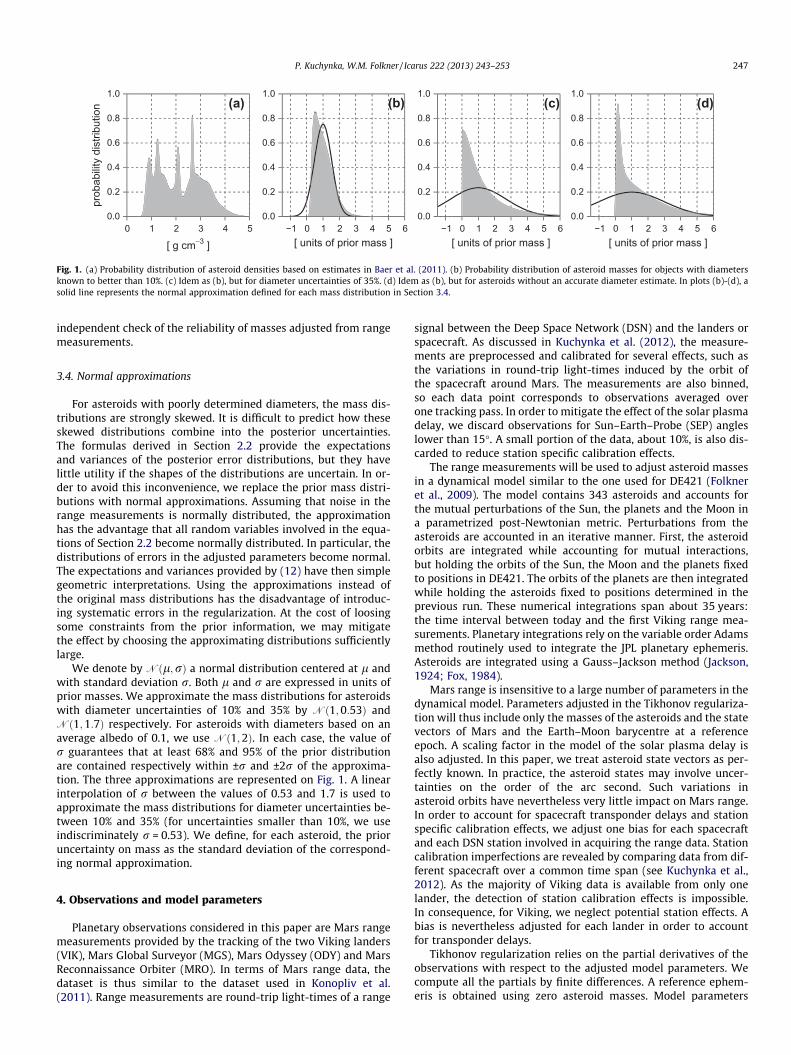
Fig. 2 represents estimated systematic errors, committed onasteroid masses, computed for a model containing only the 343asteroids usually accounted in the JPL planetary ephemeris (e.g.Folkner et al., 2009). For each mass, the systematic error is repre-sented in units of the standard deviation of the random error com-mitted on the same mass in the case where all 3714 asteroids arepresent in the model. We can thus compare each systematic error

[ un

its o

f ra

ndom

err

ors

]

−1

0

1

asteroid ordinal number1 50 100 150 200 250 300 343

Fig. 2. Systematic errors committed on asteroid masses by considering a reduceddynamical model with 343 asteroids instead of a full model with 3714 asteroids.Defined by Eq. (17), the systematic errors are represented as points correspondingto the components of E (bs) and as uncertainty intervals based on the square roots ofthe diagonal of Cov(bs). For an easier comparison with random errors, eachsystematic error and uncertainty is divided by the corresponding random uncer-tainty based on Cov(b), Eq. (12), and computed for the full model. The x-axiscorresponds to the rank of each asteroid in a sequence ordered by ascendingasteroid designation numbers.

with its random counterpart. The figure shows that the omission ofseveral thousands asteroids has negligible effects in terms of sys-tematic errors. Note that formal random errors are larger whenestimates are made for 3714 adjusted masses rather than only343 adjusted masses. The errors in both cases are nevertheless verysimilar. The lowest possible ratio between a random error esti-mated in the restricted model and in the full model is 0.96.

Eqs. (17) and (18) assume that all parameters are estimatedusing some prior uncertainty. For parameters other than asteroidmasses, such as biases or state vectors, the prior uncertaintiesare taken equal to infinity. Also, (17) and (18) assume weightedobservations. We weight MGS, ODY and MRO range data with aweight factor corresponding to a data uncertainty of 2 m. Rangingfrom both Viking landers is weighted assuming an uncertainty of20 m. This weighting scheme is the same as the one that will beused to actually estimate the asteroid masses.

The estimation of random uncertainties requires the inversionof a square covariance matrix with as many rows and columns asthere are estimated parameters. The inversion raises the concernof round off error, especially in the case where many asteroidsare present in the model and the number of estimated parametersthus amounts to several thousands. We invert covariance matricesusing the Estimation Subroutine Library (ESL, Bierman and Bier-man, 1984) by computing a square root information array and thenapplying a back substitution algorithm. In the case where all the3714 asteroid masses are adjusted, the condition number of the in-verted covariance matrix guarantees a result with at least 4 digitsfree from round off error.

5.2. Asteroid masses

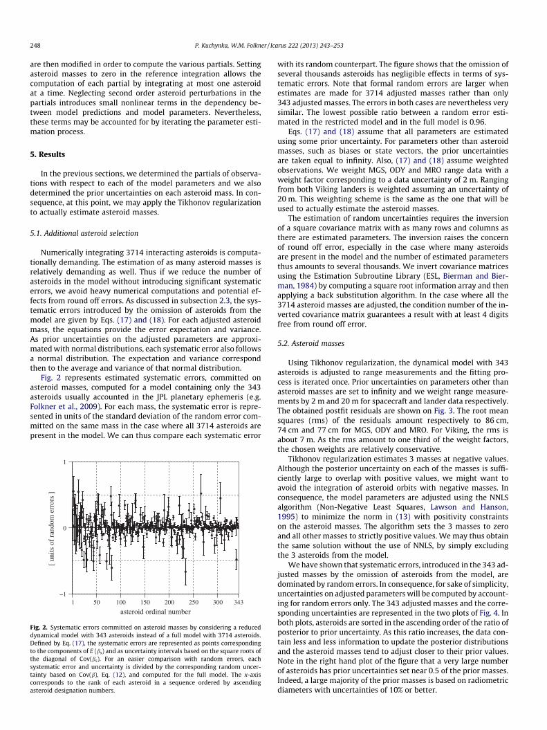
Using Tikhonov regularization, the dynamical model with 343asteroids is adjusted to range measurements and the fitting pro-cess is iterated once. Prior uncertainties on parameters other thanasteroid masses are set to infinity and we weight range measure-ments by 2 m and 20 m for spacecraft and lander data respectively.The obtained postfit residuals are shown on Fig. 3. The root meansquares (rms) of the residuals amount respectively to 86 cm,74 cm and 77 cm for MGS, ODY and MRO. For Viking, the rms isabout 7 m. As the rms amount to one third of the weight factors,the chosen weights are relatively conservative.

Tikhonov regularization estimates 3 masses at negative values.Although the posterior uncertainty on each of the masses is suffi-ciently large to overlap with positive values, we might want toavoid the integration of asteroid orbits with negative masses. Inconsequence, the model parameters are adjusted using the NNLSalgorithm (Non-Negative Least Squares, Lawson and Hanson,1995) to minimize the norm in (13) with positivity constraintson the asteroid masses. The algorithm sets the 3 masses to zeroand all other masses to strictly positive values. We may thus obtainthe same solution without the use of NNLS, by simply excludingthe 3 asteroids from the model.

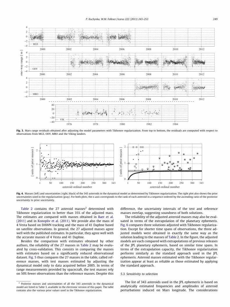
We have shown that systematic errors, introduced in the 343 ad-justed masses by the omission of asteroids from the model, aredominated by random errors. In consequence, for sake of simplicity,uncertainties on adjusted parameters will be computed by account-ing for random errors only. The 343 adjusted masses and the corre-sponding uncertainties are represented in the two plots of Fig. 4. Inboth plots, asteroids are sorted in the ascending order of the ratio ofposterior to prior uncertainty. As this ratio increases, the data con-tain less and less information to update the posterior distributionsand the asteroid masses tend to adjust closer to their prior values.Note in the right hand plot of the figure that a very large numberof asteroids has prior uncertainties set near 0.5 of the prior masses.Indeed, a large majority of the prior masses is based on radiometricdiameters with uncertainties of 10% or better.

2000 2002 2004 2006 2008 2010 2012

MGS−4

−2

0

2

4

2000 2002 2004 2006 2008 2010 2012

ODY−4

−2

0

2

4

2000 2002 2004 2006 2008 2010 2012

MRO−4

−2

0

2

4

1976 1978 1980 1982 1984

VIK−40

−20

0

20

40

one

−w

ay r

ange

[ m

]

Fig. 3. Mars range residuals obtained after adjusting the model parameters with Tikhonov regularization. From top to bottom, the residuals are computed with respect toobservations from MGS, ODY, MRO and the Viking landers.

asteroid ordinal number asteroid ordinal number1 50 100 150 200 250 300 343 1 50 100 150 200 250 300 343

[ un

its o

f pr

ior

mas

ses

]

0

1

2

[ un

its o

f pr

ior

mas

ses

]

0

1

2

Fig. 4. Masses (left) and uncertainties (right, black) of the 343 asteroids in the dynamical model as determined by Tikhonov regularization. The right plot also shows the prioruncertainties used in the regularization (gray). For both plots, the x-axis corresponds to the rank of each asteroid in a sequence ordered by the ascending ratio of the posterioruncertainty to prior uncertainty.

P. Kuchynka, W.M. Folkner / Icarus 222 (2013) 243–253 249

Table 2 contains the 27 asteroid masses2 determined withTikhonov regularization to better than 35% of the adjusted mass.The estimates are compared with masses obtained in Baer et al.(2011) and in Konopliv et al. (2011). We provide also the mass of4 Vesta based on DAWN tracking and the mass of 41 Daphne basedon satellite observations. In general, the 27 adjusted masses agreewell with the published estimates. In particular, they agree well withthe accurate masses of 4 Vesta and 41 Daphne.

Besides the comparison with estimates obtained by otherauthors, the reliability of the 27 masses in Table 2 may be evalu-ated by cross-validation. This consists in comparing the masseswith estimates based on a significantly reduced observationaldataset. Fig. 5 thus compares the 27 masses in the table, called ref-erence masses, with test masses estimated by adjusting thedynamical model only to data acquired before 2005. In terms ofrange measurements provided by spacecraft, the test masses relyon 50% fewer observations than the reference masses. Despite this

2 Posterior masses and uncertainties of all the 343 asteroids in the dynamicalmodel are listed in Table 3, available in the electronic version of this paper. The tablecontains also the various prior values used in the Tikhonov regularization.

difference, the uncertainty intervals of the test and referencemasses overlap, suggesting soundness of both solutions.

The reliability of the adjusted asteroid masses may also be eval-uated in terms of the extrapolation of the planetary ephemeris.Fig. 6 compares three solutions adjusted with Tikhonov regulariza-tion. Except for shorter time spans of observations, the three ad-justed models were obtained in exactly the same way as thesolution leading to the masses of Table 2. In the figure, the adjustedmodels are each compared with extrapolations of previous releasesof the JPL planetary ephemeris, based on similar time spans. Interms of the extrapolation capacity, the Tikhonov regularizationperforms similarly as the standard approach used in the JPLephemeris. Asteroid masses estimated with the Tikhonov regular-ization appear at least as reliable as those estimated by applyingthe standard approach.

5.3. Sensitivity to selection

The list of 343 asteroids used in the JPL ephemeris is based onanalytically estimated frequencies and amplitudes of asteroidperturbations induced on Mars longitude. The considerations

Table 2Asteroid masses estimated by Tikhonov regularization to better than 35%. Each mass appears with its formal uncertainty. The third column provides an estimate of the maximumsystematic error induced by asteroids omitted from the dynamical model. The maximum accounts for both the expectation and the standard deviation of the systematic error. Ifavailable, the table provides also astrometric mass determinations from Baer et al. (2011) and determinations from Konopliv et al. (2011) based on Mars range observations. Thelast column contains the mass of 4 Vesta based on DAWN tracking and the mass of 41 Daphne based on the imaging of its satellite.

Asteroid GM (km3 s�2) thispaper

Systematicerror

GM (km3 s�2)Baer et al. (2011)

GM (km3 s�2) Konopliv et al.(2011)

GM (km3 s�2)s/c tracking or binary

1 Ceres 62.78 ± 0.38 ±0.18 63.13 ± 0.10 62.10 ± 0.432 Pallas 13.50 ± 0.28 ±0.08 13.40 ± 0.86 13.73 ± 0.343 Juno 1.79 ± 0.11 ±0.09 1.91 ± 0.31 1.61 ± 0.124 Vesta 17.32 ± 0.11 ±0.03 17.25 ± 0.07 17.38 ± 0.27 17.28814 ± 0.00007a

6 Hebe 0.56 ± 0.13 ±0.06 0.85 ± 0.09 0.89 ± 0.227 Iris 0.99 ± 0.11 ±0.04 1.08 ± 0.06 0.73 ± 0.188 Flora 0.29 ± 0.05 ±0.02 0.44 ± 0.06 0.27 ± 0.069 Metis 0.46 ± 0.09 ±0.03 0.76 ± 0.15 0.44 ± 0.1410 Hygiea 7.01 ± 0.56 ±0.17 5.78 ± 0.10 5.97 ± 1.0313 Egeria 0.82 ± 0.22 ±0.16 1.06 ± 0.2914 Irene 0.44 ± 0.09 ±0.02 0.46 ± 0.11 0.25 ± 0.1115 Eunomia 1.74 ± 0.19 ±0.05 2.12 ± 0.02 1.88 ± 0.2016 Psyche 1.18 ± 0.28 ±0.09 1.51 ± 0.06 1.65 ± 0.4618 Melpomene 0.27 ± 0.07 ±0.0319 Fortuna 0.52 ± 0.06 ±0.02 0.55 ± 0.05 0.42 ± 0.0723 Thalia 0.11 ± 0.04 ±0.01 0.15 ± 0.0929 Amphitrite 0.69 ± 0.16 ±0.10 1.01 ± 0.04 0.98 ± 0.2031 Euphrosyne 1.46 ± 0.49 ±0.33 3.88 ± 1.3141 Daphne 0.52 ± 0.12 ±0.06 0.56 ± 0.23 0.42 ± 0.01b

42 Isis 0.10 ± 0.03 ±0.0152 Europa 2.22 ± 0.55 ±0.16 1.51 ± 0.10 1.48 ± 1.1188 Thisbe 0.75 ± 0.22 ±0.09 1.22 ± 0.0796 Aegle 0.53 ± 0.18 ±0.04324 Bamberga 0.68 ± 0.05 ±0.03 0.71 ± 0.13511 Davida 1.97 ± 0.56 ±0.46 2.52 ± 0.13 1.14 ± 0.79532 Herculina 0.86 ± 0.18 ±0.08 0.66 ± 0.37704 Interamnia 2.63 ± 0.46 ±0.32 2.59 ± 0.12 2.65 ± 0.87

a Russell et al. (2012).b Merline et al., private communication in Carry (2012).

0.0

0.5

1.0

1.5

2.0

2.5

3.0

[ un

its o

f pr

ior

mas

ses

]

1 C

eres

2 Pa

llas

3 Ju

no

4 Ve

sta

6 H

ebe

7 Ir

is

8 Fl

ora

9 M

etis

10 H

ygie

a

13 E

geri

a

14 I

rene

15 E

unom

ia

16 P

sych

e

18 M

elpo

men

e

19 F

ortu

na

23 T

halia

29 A

mph

itrite

31 E

uphr

osyn

e

41 D

aphn

e

42 I

sis

52 E

urop

a

88 T

hisb

e

96 A

egle

324

Bam

berg

a

511

Dav

ida

532

Her

culin

a

704

Inte

ram

nia

1 C

eres

2 Pa

llas

4 Ve

sta

1.32

1.33

1.34

1.35

1.20

1.25

1.30

2.10

2.15

2.20

2.25

Fig. 5. Comparison of asteroid masses and uncertainties obtained in different solutions. Each mass and uncertainty is represented by a vertical line centered at the estimatedvalue and spanning, above and below the value, one standard deviation of the formal uncertainty. In gray, the 27 masses from Table 2 determined using 343 asteroids fitted toall available data. Left of each gray line, masses obtained with the same model, but using only range observations acquired before 2005. Right of each gray line, massesobtained with a different list of asteroids adjusted to all available data. The three rightmost plots represent enlargements of the main plot for 1 Ceres, 2 Pallas and 4 Vesta.

250 P. Kuchynka, W.M. Folkner / Icarus 222 (2013) 243–253

involved in the compilation of the list are thus nontrivial. We haveseen in Section 5.1, that the list guarantees systematic errorssmaller than random errors. It is interesting to investigate to whatextent the systematic errors, and, in consequence, the quality ofthe adjusted masses, depend on a particular list of asteroids usedin the model.

A simple approach to determine a new list of asteroids is to esti-mate the amplitudes of the individual asteroid perturbations in-duced on the range data. We define each perturbation as theproduct of the asteroid’s mass with the corresponding partial ofobservations. Amplitude will be estimated from the maximumreached by the perturbation during the time interval spanned bydata. A significant part of a perturbation may be absorbed into

small changes in initial conditions of Earth and Mars. Thus theamplitudes are computed after adjusting all model parameters, ex-cept the asteroid masses, in order to reduce the least squares ofeach perturbation. Partials and prior masses have been computedin Section 4 for all the 3714 asteroids. We may thus directly com-pile a list of the 300 most perturbing objects among the 3714 aster-oids. Using Eqs. (17) and (18), we estimate the systematic errorsinduced by omitting from the model all asteroids but the 300 inthe list. The systematic errors are larger than for the previouslyconsidered 343 asteroids. Nevertheless, for almost all asteroids,the systematic errors are still smaller than their random counter-parts. The new list thus appears as a viable alternative to the usual343 asteroids.

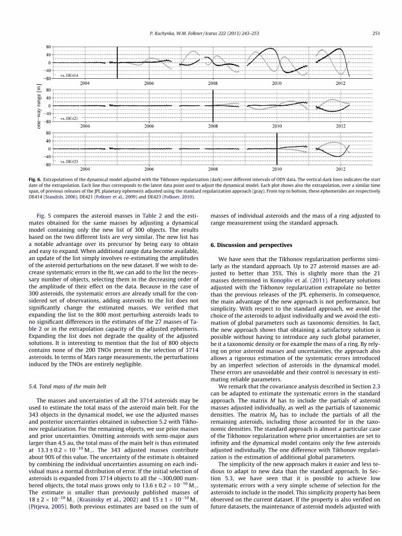
Fig. 6. Extrapolations of the dynamical model adjusted with the Tikhonov regularization (dark) over different intervals of ODY data. The vertical dark lines indicates the startdate of the extrapolation. Each line thus corresponds to the latest data point used to adjust the dynamical model. Each plot shows also the extrapolation, over a similar timespan, of previous releases of the JPL planetary ephemeris adjusted using the standard regularization approach (gray). From top to bottom, these ephemerides are respectivelyDE414 (Standish, 2006), DE421 (Folkner et al., 2009) and DE423 (Folkner, 2010).

P. Kuchynka, W.M. Folkner / Icarus 222 (2013) 243–253 251

Fig. 5 compares the asteroid masses in Table 2 and the esti-mates obtained for the same masses by adjusting a dynamicalmodel containing only the new list of 300 objects. The resultsbased on the two different lists are very similar. The new list hasa notable advantage over its precursor by being easy to obtainand easy to expand. When additional range data become available,an update of the list simply involves re-estimating the amplitudesof the asteroid perturbations on the new dataset. If we wish to de-crease systematic errors in the fit, we can add to the list the neces-sary number of objects, selecting them in the decreasing order ofthe amplitude of their effect on the data. Because in the case of300 asteroids, the systematic errors are already small for the con-sidered set of observations, adding asteroids to the list does notsignificantly change the estimated masses. We verified thatexpanding the list to the 800 most perturbing asteroids leads tono significant differences in the estimates of the 27 masses of Ta-ble 2 or in the extrapolation capacity of the adjusted ephemeris.Expanding the list does not degrade the quality of the adjustedsolutions. It is interesting to mention that the list of 800 objectscontains none of the 200 TNOs present in the selection of 3714asteroids. In terms of Mars range measurements, the perturbationsinduced by the TNOs are entirely negligible.

5.4. Total mass of the main belt

The masses and uncertainties of all the 3714 asteroids may beused to estimate the total mass of the asteroid main belt. For the343 objects in the dynamical model, we use the adjusted massesand posterior uncertainties obtained in subsection 5.2 with Tikho-nov regularization. For the remaining objects, we use prior massesand prior uncertainties. Omitting asteroids with semi-major axeslarger than 4.5 au, the total mass of the main belt is thus estimatedat 13.3 ± 0.2 � 10�10 M�. The 343 adjusted masses contributeabout 90% of this value. The uncertainty of the estimate is obtainedby combining the individual uncertainties assuming on each indi-vidual mass a normal distribution of error. If the initial selection ofasteroids is expanded from 3714 objects to all the �300,000 num-bered objects, the total mass grows only to 13.6 ± 0.2 � 10�10 M�.The estimate is smaller than previously published masses of18 ± 2 � 10�10 M� (Krasinsky et al., 2002) and 15 ± 1 � 10�10 M�(Pitjeva, 2005). Both previous estimates are based on the sum of

masses of individual asteroids and the mass of a ring adjusted torange measurement using the standard approach.

6. Discussion and perspectives

We have seen that the Tikhonov regularization performs simi-larly as the standard approach. Up to 27 asteroid masses are ad-justed to better than 35%. This is slightly more than the 21masses determined in Konopliv et al. (2011). Planetary solutionsadjusted with the Tikhonov regularization extrapolate no betterthan the previous releases of the JPL ephemeris. In consequence,the main advantage of the new approach is not performance, butsimplicity. With respect to the standard approach, we avoid thechoice of the asteroids to adjust individually and we avoid the esti-mation of global parameters such as taxonomic densities. In fact,the new approach shows that obtaining a satisfactory solution ispossible without having to introduce any such global parameter,be it a taxonomic density or for example the mass of a ring. By rely-ing on prior asteroid masses and uncertainties, the approach alsoallows a rigorous estimation of the systematic errors introducedby an imperfect selection of asteroids in the dynamical model.These errors are unavoidable and their control is necessary in esti-mating reliable parameters.

We remark that the covariance analysis described in Section 2.3can be adapted to estimate the systematic errors in the standardapproach. The matrix M has to include the partials of asteroidmasses adjusted individually, as well as the partials of taxonomicdensities. The matrix Mg has to include the partials of all theremaining asteroids, including those accounted for in the taxo-nomic densities. The standard approach is almost a particular caseof the Tikhonov regularization where prior uncertainties are set toinfinity and the dynamical model contains only the few asteroidsadjusted individually. The one difference with Tikhonov regulari-zation is the estimation of additional global parameters.

The simplicity of the new approach makes it easier and less te-dious to adapt to new data than the standard approach. In Sec-tion 5.3, we have seen that it is possible to achieve lowsystematic errors with a very simple scheme of selection for theasteroids to include in the model. This simplicity property has beenobserved on the current dataset. If the property is also verified onfuture datasets, the maintenance of asteroid models adjusted with

252 P. Kuchynka, W.M. Folkner / Icarus 222 (2013) 243–253

Tikhonov regularization could become very straightforward. Witha sufficiently large selection of asteroids, the maintenance even be-comes unnecessary. New observations can be accommodated,without any changes, by the same model.

The new approach appears suitable to effectively and rapidlyevaluate the information content of synthetic observations withrespect to asteroid masses. The evaluation involves simply theinversion of a square covariance matrix. In a future study, the ap-proach could thus be used to estimate the constraints on asteroidmasses as a function of the accuracy and time span of future rangedata. Similarly, it could estimate the information content as a func-tion of various parameters considered in the design and planningof future missions. Performing such experiments with the standardapproach is not practical as it requires, for each set of syntheticdata, empirically updating the list of individually adjusted masses.

The set of prior constraints used in this study is relatively loose.The constraints could be tightened by simply increasing the weightof the range measurements with respect to the prior constraints.The weights applied in Section 5.2 are conservative and could bemoderately increased without introducing significant systematicerrors. Unfortunately, the optimal weighting depends on theamplitude of unknown systematic errors such as errors fromimperfect modelling of the solar plasma delay. Prior constraintscould be improved by updating the prior uncertainties with pub-lished mass estimates obtained independently of planetary range.Nevertheless, preliminary experiments have shown that reducingthe prior uncertainties on a few asteroids only marginally im-proves the posterior uncertainties on other asteroids. Better poten-tial for improvement lies in accounting, in the prior uncertainties,for different average densities in the C and S taxonomic classes.Contrary to the individually published masses, this information af-fects a large number of asteroids and could thus improve posterioruncertainties to a larger extent.

7. Conclusion

We present a new approach to estimate asteroid masses fromplanetary range measurements. The approach is based on Tikhonovregularization, a least squares estimation where all asteroidmasses are considered individually and adjusted using realisticprior constraints. The constraints are provided mainly by radio-metric estimations of asteroid diameters. The approach providessignificant advantages over the standard methodology of estimat-ing asteroid masses from range. It simplifies regularization byavoiding the distinction between masses adjusted individuallyand masses determined from taxonomic densities. It also allowsa quantitative estimation of the systematic errors introduced byasteroids not accounted in the dynamical model. We have shownthat, for currently available Mars range measurements, even a sim-ple scheme of selection of the asteroids to include in the modelguarantees systematic errors smaller than random errors.

The new approach could significantly simplify the maintenanceof the asteroid model in the JPL planetary ephemeris and the adap-tation of the model to future planetary range data.

Acknowledgments

We thank Alex S. Konopliv for reduced NASA Mars spacecraftranging and Robert A. Jacobson for providing a basic asteroid inte-grator code. The publication also benefits from previous efforts car-ried out in collaboration with Jacques Laskar and Agnès Fienga.This research was supported by an appointment to the NASA Post-doctoral Program at the Jet Propulsion Laboratory, administered byOak Ridge Associated Universities through a contract with NASA.The publication uses data from the Wide-field Infrared Survey

Explorer (WISE), a joint project of the University of California, LosAngeles, and the Jet Propulsion Laboratory/California Institute ofTechnology.

Appendix A. Supplementary data

Supplementary data associated with this article can be found, inthe online version, at http://dx.doi.org/10.1016/j.icarus.2012.11.003.

References

Baer, J., Chesley, S.R., Matson, R.D., 2011. Astrometric masses of 26 Asteroids andobservations on asteroid porosity. Astron. J. 141 (May), 143-1–143-12.

Bickel, P.J., Doksum, K.A., 2001. Appendix A & B. In: Mathematical Statistics: BasicIdeas and Selected Topics, vol. I.

Bierman, G.J., 1977. Covariance Analysis of Effects Due to Mismodeled Variables andIncorrect Filter a Priori Statistics. In: Factorization Methods for DiscreteSequential Estimation. Academic Press (Chapter VIII).

Bierman, G.J., Bierman, K.H., 1984. Estimation Subroutine Library: (Preliminary)User Guide. FEA Report No. 81584.

Bus, S.J., Vilas, F., Barucci, M.A., 2002. Visible-wavelength spectroscopy of asteroids.Asteroids III, 169–182.

Carry, B., 2012. Density of asteroids. Planet. Space Sci., in press. Available from:<arXiv:1203.4336>.

Descamps, P., Marchis, F., Michalowski, T., Vachier, F., Colas, F., Berthier, J.,Assafin, M., Dunckel, P.B., Polinska, M., Pych, W., Hestroffer, D., Miller, K.P.M.,Vieira-Martins, R., Birlan, M., Teng-Chuen-Yu, J.-P., Peyrot, A., Payet, B.,Dorseuil, J., Léonie, Y., Dijoux, T., 2007. Figure of the double Asteroid 90Antiope from adaptive optics and lightcurve observations. Icarus 187 (April),482–499.

Fienga, A. et al., 2009. INPOP08, a 4-D planetary ephemeris: From asteroid and time-scale computations to ESA Mars Express and Venus Express contributions.Astron. Astrophys. 507 (December), 1675–1686.

Fienga, A. et al., 2011. The INPOP10a planetary ephemeris and its applications infundamental physics. Celest. Mech. Dynam. Astron. 111 (November), 363–385.

Fienga, A., Manche, H., Laskar, J., Gastineau, M., 2008. INPOP06: A new numericalplanetary ephemeris. Astron. Astrophys. 477 (January), 315–327.

Folkner, W.M., 2010. Planetary ephemeris DE423 fit to messenger encounters withMercury. JPL IOM 343R-08-003.

Folkner, W.M., Williams, J.G., Boggs, D.H., 2009. The Planetary and Lunar EphemerisDE 421. IPN Progress Report 42-178.

Fox, K., 1984. Numerical integration of the equations of motion of celestialmechanics. Celest. Mech. 33 (June), 127–142.

Hansen, P.C., 1977. Direct Regularization Methods. In: Rank-Deficient and DiscreetIll-posed Problems. SIAM (Chapter 5).

Harris, A.W., Lagerros, J.S.V., 2002. Asteroids in the thermal infrared. Asteroids III,205–218.

Hellings, R.W. et al., 1983. Experimental test of the variability of G using Vikinglander ranging data. Phys. Rev. Lett. 51 (October), 1609–1612.

Jackson, J., 1924. Note on the numerical integration of d2x/dt2 = f(x, t). Mon. Not. R.Astron. Soc. 84 (June), 602–606.

Konopliv, A.S., Yoder, C.F., Standish, E.M., Yuan, D.-N., Sjogren, W.L., 2006. A globalsolution for the Mars static and seasonal gravity, Mars orientation, Phobos andDeimos masses, and Mars ephemeris. Icarus 182 (May), 23–50.

Konopliv, A.S., Asmar, S.W., Folkner, W.M., Karatekin, Ö., Nunes, D.C., Smrekar, S.E.,Yoder, C.F., Zuber, M.T., 2011. Mars high resolution gravity fields from MRO,Mars seasonal gravity, and other dynamical parameters. Icarus 211 (January),401–428.

Krasinsky, G.A., Pitjeva, E.V., Vasilyev, M.V., Yagudina, E.I., 2002. Hidden Mass in theasteroid belt. Icarus 158 (July), 98–105.

Kuchynka, P., 2010. Étude des perturbations induites par les astéroïdes sur lesmouvements des planètes et des sondes spatiales autour du point de LagrangeL2. Ph.D. thesis, Observatoire de Paris, France, thèse dirigée par J. Laskar et A.Fienga.

Kuchynka, P., Laskar, J., Fienga, A., Manche, H., 2010. A ring as a model of themain belt in planetary ephemerides. Astron. Astrophys. 514 (May), A96-1–A96-17.

Kuchynka, P., Folkner, W.M., Konopliv, A.S., 2012. Station Specific Errors in MarsRanging Measurements. IPN Progress Report 42-189.

Lawson, C.L., Hanson, R.J., 1995. Solving Least Squares Problems. SIAM, Philadelphia.Masiero, J.R. et al., 2011. Main belt asteroids with WISE/NEOWISE. I. Preliminary

albedos and diameters. Astrophys. J. 741 (November), 68-1–68-20.Müller, T.G., Blommaert, J.A.D.L., 2004. 65 Cybele in the thermal infrared: Multiple

observations and thermophysical analysis. Astron. Astrophys. 418 (April), 347–356.

Pitjeva, E.V., 2005. High-precision ephemerides of planets-EPM and determinationof some astronomical constants. Solar System Res. 39 (May), 176–186.

Pitjeva, E.V., 2010. EPM ephemerides and relativity. In: Klioner, S.A., Seidelmann,P.K., Soffel, M.H. (Eds.), IAU Symposium, vol. 261. pp. 170–178.

Russell, C.T. et al., 2012. Dawn at Vesta: Testing the protoplanetary paradigm.Science 336 (May), 684–686.

P. Kuchynka, W.M. Folkner / Icarus 222 (2013) 243–253 253

Shepard, M.K., Clark, B.E., Nolan, M.C., Howell, E.S., Magri, C., Giorgini, J.D., Benner,L.A.M., Ostro, S.J., Harris, A.W., Warner, B., Pray, D., Pravec, P., Fauerbach, M.,Bennett, T., Klotz, A., Behrend, R., Correia, H., Coloma, J., Casulli, S., Rivkin, A.,2008. A radar survey of M- and X-class asteroids. Icarus 195 (May), 184–205.

Somenzi, L., Fienga, A., Laskar, J., Kuchynka, P., 2010. Determination of asteroidmasses from their close encounters with Mars. Planet. Space Sci. 58 (April),858–863.

Standish, E.M., 2006. JPL Planetary Ephemerides, DE414. JPL IOM 343R-06-002.Standish, E.M., Hellings, R.W., 1989. A determination of the masses of Ceres, Pallas,

and Vesta from their perturbations upon the orbit of Mars. Icarus 80 (August),326–333.

Stansberry, J., Grundy, W., Brown, M., Cruikshank, D., Spencer, J., Trilling, D., Margot,J.-L., 2008. Physical properties of Kuiper belt and Centaur objects: Constraintsfrom Spitzer Space Telescope. In: The Solar System Beyond Neptune. p. 161.

Tedesco, E.F., Noah, P.V., Noah, M., Price, S.D., 2002. The supplemental IRAS minorplanet survey. Astron. J. 123 (February), 1056–1085.

Tedesco, E.F., Noah, P.V., Noah, M., Price, S.D., 2004a. IRAS Minor Planet Survey V6.0.NASA Planetary Data System 12.

Tedesco, E.T., Egan, M.P., Price, S.D., 2004b. MSX Infrared Minor Planet Survey V1.0.NASA Planetary Data System 3.

Verma, A.K., Fienga, A., Laskar, J., Issautier, K., Manche, H., Gastineau, M., 2012.Electron density distribution and solar plasma correction of radio signals usingMGS, MEX and VEX spacecraft navigation data and its application to planetaryephemerides. Astron. Astrophys., submitted for publication. Available from:<arXiv:1206.5667>.

Williams, J.G., 1984. Determining asteroid masses from perturbations on Mars.Icarus 57 (January), 1–13.