6th International Conference on Advances in Experimental Structural Engineering 11th International Workshop on Advanced Smart Materials and Smart Structures Technology August 1-2, 2015, University of Illinois, Urbana-Champaign, United States  

A New Force-Based Formulation of Equations of Motion  

for Hybrid Simulation B.Forouzan1, N.Nakata2 1 Graduate student, Dept. of Civil and Environmental Engineering, Clarkson University, Potsdam, United States.

E-mail: forouzb@clarkson.edu 2 Associate Professor, Dept. of Civil and Environmental Engineering, Clarkson University, Potsdam, United States. E-mail: nnakata@clarkson.edu

ABSTRACT Hybrid simulation is a versatile, powerful and economical method for modelling large and complex structural systems, combining numerical and experimental models. While the hybrid simulation technique has been used in seismic simulation, application to the other dynamic loads such as strong wind, hurricane and tsunami have been limited. One of the reasons is because displacement based formulation and control used in the conventional hybrid simulation are not always suitable. This study explores a force-based formulation in hybrid simulation. In particular, a new numerical integration method, called weighted Predictor-Corrector force-based algorithm is proposed herein. In the proposed algorithm, force is first predicted in an intermediate step, according to responses at the previous step. The predicted force is imposed to the experiment using force control, and the corresponding displacement is then measured and sent back to the numerical algorithm. Responses at the next step are calculated based on the measured displacement through a correction procedure. Thus, the proposed algorithm enables force-based formulation and allows for force control in hybrid simulation. A preliminary numerical simulation is performed to verify applicability of this proposed algorithm. The numerical simulation demonstrates that this algorithm provides stable and accurate results in force-based hybrid simulation. This paper presents details of the algorithm and the preliminary numerical results. KEYWORDS: Hybrid simulation, Hazard simulation, Force-based formulation, Predictor-corrector algorithm, Force control. 1. INTRODUCTION Natural hazards, such as earthquakes, tsunamis and strong winds, have caused tremendous human suffering and damage to structures. In order to reduce the effects of these phenomena, it is imperative to improve knowledge and understanding of the response of structures to such natural events. One of the effective approaches for investigation of structural responses is hybrid simulation technique. Hybrid simulation provides an alternative for dynamic testing of structural systems, combining physical testing and computer modeling (Takanashi et al., 1975, Mahin and Shing, 1985, Takanashi and Nakashima, 1987). In hybrid simulation, structural elements that are difficult to model numerically are generally tested in experiment. The conventional hybrid simulation technique is displacement-based; procedure is driven by displacement. The general procedure in the displacement-based hybrid simulation consists of three phases. In the first phase, displacement of the structure is calculated numerically using a time step integration of equations of motion as a target displacement. In the second phase the target displacement is imposed to the test specimen and the corresponding force is measured. In the last phase, the measured force is fed back to the equations of motion to update responses at the current step. While this conventional hybrid simulation technique is suitable and has been used in various applications, it has some limitations. For example, the displacement control with extremely rigid structure is challenging and the experimental errors are unavoidable because of the displacement resolution. Furthermore, simulation of structures subjected to hydrodynamic loads, such as tsunamis, storm surge and braking waves require strict force equilibrium conditions between fluid and structure as opposed to displacement compatibilities. To overcome these limitations and needs, this study investigates a new force-based hybrid simulation technique as a potential approach. In this paper, a force-based predictor-corrector numerical integration algorithm is proposed. The proposed algorithm consists of three phases. In the first phase, force is predicted based on the responses at the previous

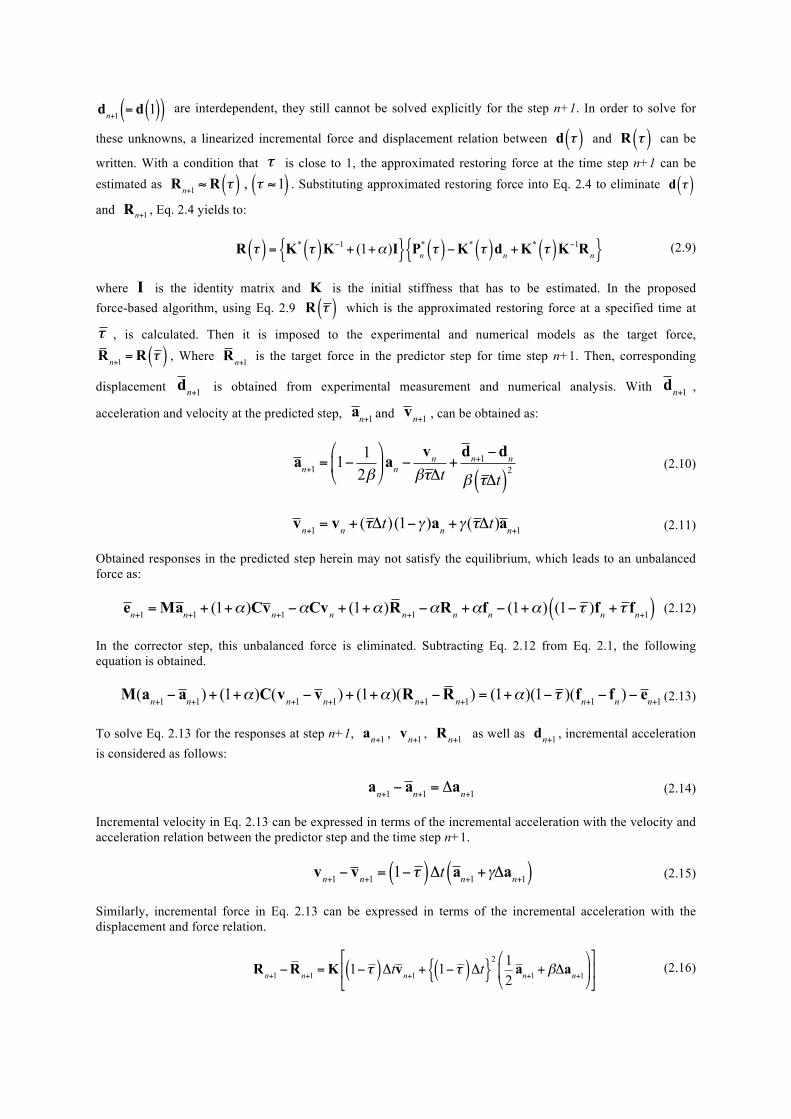
step. In the second phase, the predicted force is imposed to the experiment using force control technique, and the corresponding displacement is measured. In the last phase, the measured displacement is sent back to the numerical algorithm and responses at the next step are updated based on the measured displacement through a corrector procedure. The main difference between the two approaches is that as described above, the procedure in the force-based algorithm is driven by the force. This paper presents the details of the proposed force-based predictor-corrector algorithm and a preliminary numerical simulation. In addition future studies are discussed. 2. FORCE-BASED PREDICTOR-CORRECTOR NUMERICAL ALGORITHM This section presents the mathematical details and procedure of the force-based predictor-corrector numerical time step integration algorithm. In the proposed force-based algorithm, the equations of motion of a structural system is expressed as (Hilber et al., 1977):

Man+1 + (1+α)Cvn+1 −αCvn + (1+α)Rn+1 −αRn = (1+α)fn+1 −αfn (2.1) where and are the mass matrix and damping matrix, respectively; is the acceleration vector; is the velocity vector; is the restoring force vector; is the excitation force vector; α is the integration parameter (−1 3<α ≤ 0 ); and the subscript n denotes the time step. Suppose responses at the time step n and the

input forces are given, unknown responses at the time step n+1 that have to be solved are , ,

and , where is the displacement vector. Displacement and velocity between the time steps n and n+1 can be expressed as follows:

d τ( ) = dn +τΔtvn + τΔt( )2 12−β

#

$%

&

'(an +βan+1

)*+

,+

-.+

/+ (2.2)

  v τ( ) = vn +τΔt(1−γ )an +τΔtγan+1                                                       (2.3)

where τ is a variable between 0 and 1 (0 < τ ≤1); Δt is the time interval; and d τ( ) and v τ( ) are the

interpolated displacement and velocity. Two parameters β and γ in Eqs. 2.2 and 2.3 are defined as β = (1−α)2 / 2 and γ = (1− 2α) / 2 . By eliminating and in Eq. 2.1 using Eqs. 2.2 and 2.3, the equations of motion can be rewritten as:

K* τ( )d τ( )+ (1+α)Rn+1 = Pn* τ( ) (2.4)

where

(2.5)

(2.6)

(2.7)

(2.8)

Note that the terms with the superscript * are introduced for the sake of simplicity; they can be expressed with the known terms. Now, Eq. 2.4 has only two unknowns,   and . However, because and

M C a vR f

an+1 vn+1 dn+1Rn+1 d

an+1 vn+1

K* τ( ) = M(τΔt)2β

+(1+α)γCτΔtβ

Pn* τ( ) = (1+α)fn+1 −αfn − (1+α)Cv*n +αCvn +K* τ( )d*n τ( )+αRn

d*n τ( ) = dn +τΔt vn +(τΔt)2

2(1− 2β)an

v*n = vn +Δt (1−γ )an

d τ( ) Rn+1 Rn+1

are interdependent, they still cannot be solved explicitly for the step n+1. In order to solve for

these unknowns, a linearized incremental force and displacement relation between and can be

written. With a condition that is close to 1, the approximated restoring force at the time step n+1 can be estimated as . Substituting approximated restoring force into Eq. 2.4 to eliminate

and , Eq. 2.4 yields to:

(2.9)

where is the identity matrix and K is the initial stiffness that has to be estimated. In the proposed force-based algorithm, using Eq. 2.9 which is the approximated restoring force at a specified time at

, is calculated. Then it is imposed to the experimental and numerical models as the target force, , Where is the target force in the predictor step for time step n+1. Then, corresponding

displacement is obtained from experimental measurement and numerical analysis. With ,

acceleration and velocity at the predicted step, and , can be obtained as:

(2.10)

(2.11)

Obtained responses in the predicted step herein may not satisfy the equilibrium, which leads to an unbalanced force as:

en+1 =Man+1 + (1+α)Cvn+1 −αCvn + (1+α)Rn+1 −αRn +αfn − (1+α) (1−τ )fn +τ fn+1( ) (2.12)

In the corrector step, this unbalanced force is eliminated. Subtracting Eq. 2.12 from Eq. 2.1, the following equation is obtained.

(2.13)

To solve Eq. 2.13 for the responses at step n+1, , , as well as , incremental acceleration is considered as follows:

(2.14)

Incremental velocity in Eq. 2.13 can be expressed in terms of the incremental acceleration with the velocity and acceleration relation between the predictor step and the time step n+1.

(2.15)

Similarly, incremental force in Eq. 2.13 can be expressed in terms of the incremental acceleration with the displacement and force relation.

(2.16)

dn+1 = d 1( )( )d τ( ) R τ( )

τRn+1 ≈ R τ( ) , τ ≈1( ) d τ( )

Rn+1

R τ( ) = K* τ( )K−1 + (1+α)I{ } Pn* τ( )−K* τ( )dn +K* τ( )K−1Rn{ }

IRn+1 =R τ( )

τRn+1 =R τ( ) Rn+1

dn+1 dn+1an+1 vn+1

an+1 = 1− 12β

"

#$

%

&'an −

vnβτΔt

+dn+1 −dnβ τΔt( )

2

vn+1 = vn + (τΔt)(1−γ )an +γ (τΔt)an+1

M(an+1 − an+1)+ (1+α)C(vn+1 − vn+1)+ (1+α)(Rn+1 −Rn+1) = (1+α)(1−τ )(fn+1 − fn )− en+1

an+1 vn+1 Rn+1 dn+1

an+1 − an+1 = Δan+1

vn+1 − vn+1 = 1−τ( )Δt an+1 +γΔan+1( )

Rn+1 −Rn+1 =K 1−τ( )Δtvn+1 + 1−τ( )Δt{ }2 12an+1 +βΔan+1

#

$%

&

'(

)

*+

,

-.

Substituting Eqs. 2.14- 2.16 into Eq. 2.13 to eliminate

, and , the incremental acceleration can be solved.

(2.17)

where express as:

(2.18)

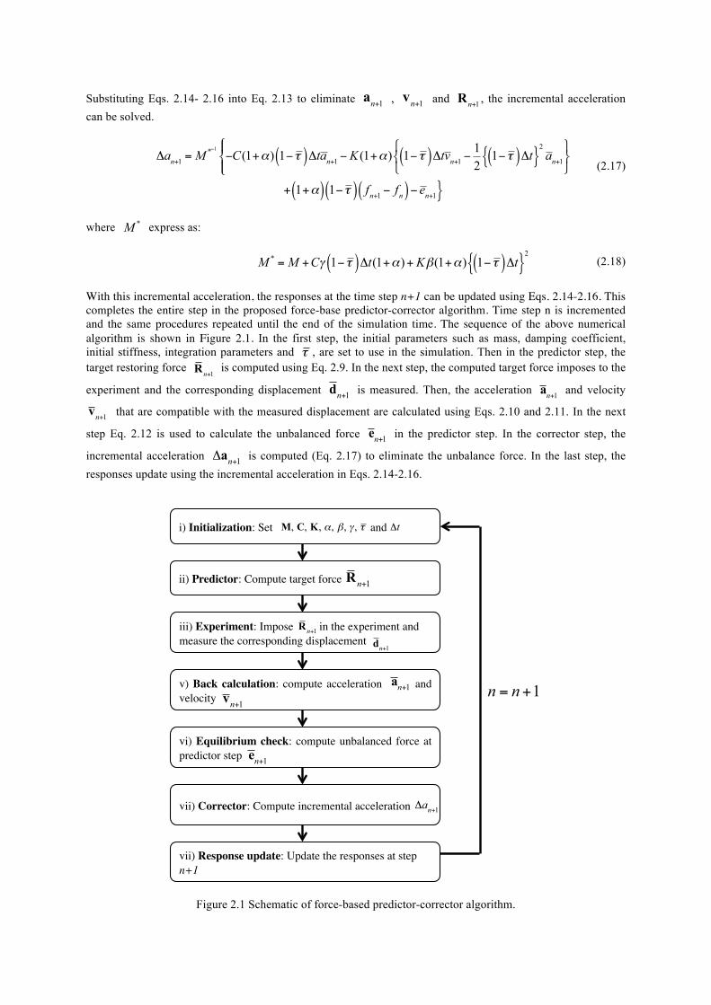
With this incremental acceleration, the responses at the time step n+1 can be updated using Eqs. 2.14-2.16. This completes the entire step in the proposed force-base predictor-corrector algorithm. Time step n is incremented and the same procedures repeated until the end of the simulation time. The sequence of the above numerical algorithm is shown in Figure 2.1. In the first step, the initial parameters such as mass, damping coefficient, initial stiffness, integration parameters and , are set to use in the simulation. Then in the predictor step, the target restoring force is computed using Eq. 2.9. In the next step, the computed target force imposes to the

experiment and the corresponding displacement is measured. Then, the acceleration and velocity

that are compatible with the measured displacement are calculated using Eqs. 2.10 and 2.11. In the next

step Eq. 2.12 is used to calculate the unbalanced force in the predictor step. In the corrector step, the

incremental acceleration is computed (Eq. 2.17) to eliminate the unbalance force. In the last step, the responses update using the incremental acceleration in Eqs. 2.14-2.16.

Figure 2.1 Schematic of force-based predictor-corrector algorithm.

an+1 vn+1 Rn+1

Δan+1 =M*−1 −C(1+α) 1−τ( )Δtan+1 − K (1+α) 1−τ( )Δtvn+1 −

121−τ( )Δt{ }

2an+1

!"#

$%&

!"'

#'

+ 1+α( ) 1−τ( ) fn+1 − fn( )− en+1}

M *

M * =M +Cγ 1−τ( )Δt(1+α)+ Kβ(1+α) 1−τ( )Δt{ }2

τRn+1

dn+1 an+1vn+1

en+1Δan+1

i) Initialization: Set and

iii) Experiment: Impose in the experiment and measure the corresponding displacement

ii) Predictor: Compute target force

v) Back calculation: compute acceleration and velocity n = n+1

M, C, K, α, β , γ , τ

Rn+1

Δt

Rn+1dn+1

an+1vn+1

vi) Equilibrium check: compute unbalanced force at predictor step en+1

vii) Corrector: Compute incremental acceleration Δan+1

vii) Response update: Update the responses at step n+1

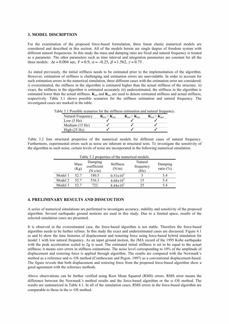
3. MODEL DISCRIPTION For the examination of the proposed force-based formulation, three linear elastic numerical models are considered and described in this section. All of the models herein are single degree of freedom system with different natural frequencies. In this study the mass and damping ratio are fixed and natural frequency is treated as a parameter. The other parameters such as time interval and integration parameters are constant for all the three models: . As stated previously, the initial stiffness needs to be estimated prior to the implementation of the algorithm. However, estimation of stiffness is challenging and estimation errors are unavoidable. In order to account for such estimation errors in the numerical simulation, three different cases with the estimation error are considered; i) overestimated, the stiffness in the algorithm is estimated higher than the actual stiffness of the structure. ii) exact, the stiffness in the algorithm is estimated accurately iii) underestimated, the stiffness in the algorithm is estimated lower than the actual stiffness. Kest and Kact are used to denote estimated stiffness and actual stiffness, respectively. Table 3.1 shows possible scenarios for the stiffness estimation and natural frequency. The investigated cases are marked in the table.

Table 3.1 Possible scenarios for the stiffness estimation and natural frequency. Natural Frequency Kest < Kact Kest = Kact Kest > Kact Low (5 Hz) ✓ ✓ ✓ Medium (15 Hz) ✓ ✓ ✓ High (25 Hz) ✓ ✓ ✓

Table 3.2 lists structural properties of the numerical models for different cases of natural frequency. Furthermore, experimental errors such as noise are inherent in structural tests. To investigate the sensitivity of the algorithm to such noise, certain levels of noise are incorporated in the following numerical simulation.

Table 3.2 properties of the numerical models. Mass

(Kg)

Damping coefficient

(N s/m)

Stiffness (N/m)

Natural frequency

(Hz)

Damping ratio (%)

Model 1 52.7 180.5 0.53×105 5 5.4 Model 2 52.7 536.3 4.68×105 15 5.4 Model 3 52.7 722 8.44×105 25 5.4

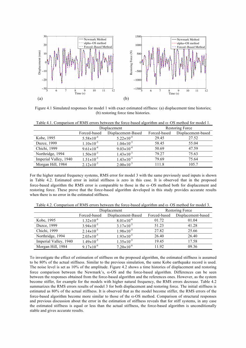
4. PRELIMINARY RESULTS AND DISSCOUTION A series of numerical simulations are performed to investigate accuracy, stability and sensitivity of the proposed algorithm. Several earthquake ground motions are used in this study. Due to a limited space, results of the selected simulation cases are presented. It is observed in the overestimated case, the force-based algorithm is not stable. Therefore the force-based algorithm needs to be further refines. In this study the exact and underestimated cases are discussed. Figure 4.1 (a and b) show the time histories of displacement and restoring force using force-based hybrid simulation for model 1 with low natural frequency. As an input ground motion, the JMA record of the 1995 Kobe earthquake with the peak acceleration scaled to 2g is used. The estimated initial stiffness is set to be equal to the actual stiffness; it means zero errors in stiffness estimations. The noise level corresponding to 10% of the amplitude of displacement and restoring force is applied through algorithm. The results are compared with the Newmark’s method as a reference and α–OS method (Combescure and Pegon, 1997) as a conventional displacement-based. The figure reveals that both displacement and restoring force from the proposed force-based algorithm show a good agreement with the reference methods. Above observations can be further verified using Root Mean Squared (RMS) errors. RMS error means the difference between the Newmark’s method results and the force-based algorithm or the α–OS method. The results are summarized in Table 4.1. In all of the simulation cases, RMS errors in the force-based algorithm are comparable to those in the α–OS method.

Δt = 0.004 sec, τ = 0.9, α = −0.25, β =1.562, γ = 0.75

(a) (b)

Figure 4.1 Simulated responses for model 1 with exact estimated stiffness: (a) displacement time histories;

(b) restoring force time histories.

Table 4.1. Comparison of RMS errors between the force-based algorithm and α–OS method for model 1. Displacement Restoring Force Forced-based Displacement-Based Forced-based Displacement-based Kobe, 1995 5.58×10-4 5.22×10-4 29.45 27.52 Duzce, 1999 1.10×10-3 1.04×10-3 58.45 55.04 Chichi, 1999 9.61×10-4 9.03×10-4 50.69 47.59 Northridge, 1994 1.50×10-3 1.43×10-3 79.27 75.63 Imperial Valley, 1940 1.51×10-3 1.43×10-3 79.69 75.64 Morgan Hill, 1984 2.12×10-3 2.00×10-3 111.8 105.7

For the higher natural frequency systems, RMS error for model 3 with the same previously used inputs is shown in Table 4.2. Estimated error in initial stiffness is zero in this case. It is observed that in the proposed force-based algorithm the RMS error is comparable to those in the α–OS method both for displacement and restoring force. These prove that the force-based algorithm developed in this study provides accurate results when there is no error in the estimated stiffness.

Table 4.2. Comparison of RMS errors between the force-based algorithm and α–OS method for model 3. Displacement Restoring Force Forced-based Displacement-Based Forced-based Displacement-based Kobe, 1995 1.32×10-6 8.01×10-6 01.72 01.04 Duzce, 1999 3.94×10-5 3.17×10-5 51.23 41.28 Chichi, 1999 2.14×10-5 1.98×10-5 27.82 25.66 Northridge, 1994 2.03×10-5 1.93×10-5 26.40 26.40 Imperial Valley, 1940 1.49×10-5 1.35×10-5 19.45 17.58 Morgan Hill, 1984 9.17×10-6 7.20×10-6 11.92 09.36

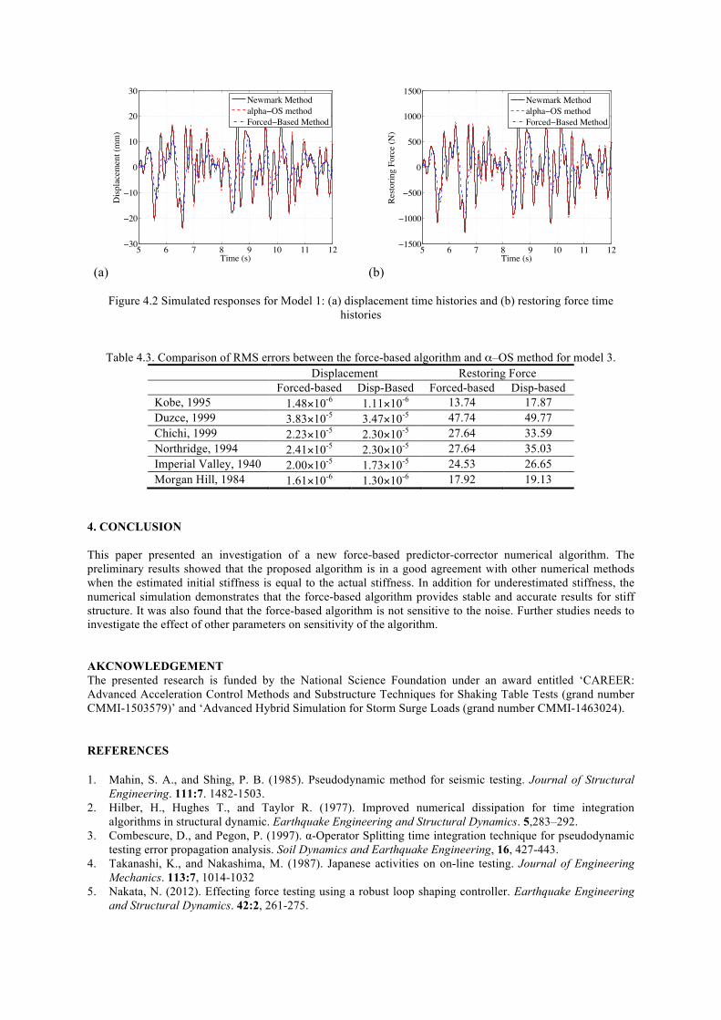
To investigate the effect of estimation of stiffness on the proposed algorithm, the estimated stiffness is assumed to be 80% of the actual stiffness. Similar to the previous simulation, the same Kobe earthquake record is used. The noise level is set as 10% of the amplitude. Figure 4.2 shows a time histories of displacement and restoring force comparison between the Newmark’s, α-OS and the force-based algorithm. Differences can be seen between the responses obtained from the force-based algorithm and the references ones. However, as the system become stiffer, for example for the models with higher natural frequency, the RMS errors decrease. Table 4.2 summarizes the RMS errors results of model 3 for both displacement and restoring force. The initial stiffness is estimated as 80% of the actual stiffness. It is observed that as the model become stiffer, the RMS errors of the force-based algorithm become more similar to those of the α-OS method. Comparison of structural responses and previous discussion about the error in the estimation of stiffness reveals that for stiff systems, in any case the estimated stiffness is equal or less than the actual stiffness, the force-based algorithm is unconditionally stable and gives accurate results.

5 6 7 8 9 10 11 12−30

−20

−10

0

10

20

30

Time (s)

Disp

lace

men

t (m

m)

Newmark Methodalpha−OS methodForced−Based Method

Student Version of MATLAB

5 6 7 8 9 10 11 12−1500

−1000

−500

0

500

1000

1500

Time (s)

Resto

ring

Forc

e (N

)

Newmark Methodalpha−OS methodForced−Based Method

Student Version of MATLAB

(a) (b)

Figure 4.2 Simulated responses for Model 1: (a) displacement time histories and (b) restoring force time

histories

Table 4.3. Comparison of RMS errors between the force-based algorithm and α–OS method for model 3. Displacement Restoring Force Forced-based Disp-Based Forced-based Disp-based Kobe, 1995 1.48×10-6 1.11×10-6 13.74 17.87 Duzce, 1999 3.83×10-5 3.47×10-5 47.74 49.77 Chichi, 1999 2.23×10-5 2.30×10-5 27.64 33.59 Northridge, 1994 2.41×10-5 2.30×10-5 27.64 35.03 Imperial Valley, 1940 2.00×10-5 1.73×10-5 24.53 26.65 Morgan Hill, 1984 1.61×10-6 1.30×10-6 17.92 19.13

4. CONCLUSION This paper presented an investigation of a new force-based predictor-corrector numerical algorithm. The preliminary results showed that the proposed algorithm is in a good agreement with other numerical methods when the estimated initial stiffness is equal to the actual stiffness. In addition for underestimated stiffness, the numerical simulation demonstrates that the force-based algorithm provides stable and accurate results for stiff structure. It was also found that the force-based algorithm is not sensitive to the noise. Further studies needs to investigate the effect of other parameters on sensitivity of the algorithm. AKCNOWLEDGEMENT The presented research is funded by the National Science Foundation under an award entitled ‘CAREER: Advanced Acceleration Control Methods and Substructure Techniques for Shaking Table Tests (grand number CMMI-1503579)’ and ‘Advanced Hybrid Simulation for Storm Surge Loads (grand number CMMI-1463024).

REFERENCES 1. Mahin, S. A., and Shing, P. B. (1985). Pseudodynamic method for seismic testing. Journal of Structural

Engineering. 111:7. 1482-1503. 2. Hilber, H., Hughes T., and Taylor R. (1977). Improved numerical dissipation for time integration

algorithms in structural dynamic. Earthquake Engineering and Structural Dynamics. 5,283–292. 3. Combescure, D., and Pegon, P. (1997). α-Operator Splitting time integration technique for pseudodynamic

testing error propagation analysis. Soil Dynamics and Earthquake Engineering, 16, 427-443. 4. Takanashi, K., and Nakashima, M. (1987). Japanese activities on on-line testing. Journal of Engineering

Mechanics. 113:7, 1014-1032 5. Nakata, N. (2012). Effecting force testing using a robust loop shaping controller. Earthquake Engineering

and Structural Dynamics. 42:2, 261-275.

5 6 7 8 9 10 11 12−30

−20

−10

0

10

20

30

Time (s)

Disp

lace

men

t (m

m)

Newmark Methodalpha−OS methodForced−Based Method

Student Version of MATLAB

5 6 7 8 9 10 11 12−1500

−1000

−500

0

500

1000

1500

Time (s)

Resto

ring

Forc

e (N

)

Newmark Methodalpha−OS methodForced−Based Method

Student Version of MATLAB