A NEW MODEL FOR REALISTIC RANDOM PERTURBATIONS …people.math.gatech.edu/~dieci/preps/DLZ-Theory.pdf · A NEW MODEL FOR REALISTIC RANDOM PERTURBATIONS OF STOCHASTIC OSCILLATORS LUCA

Version of Monday 19th January, 2015, 08:21

A NEW MODEL FOR REALISTIC RANDOM PERTURBATIONS

OF STOCHASTIC OSCILLATORS

LUCA DIECI, WUCHEN LI, HAOMIN ZHOU

Abstract. Classical theories predict that solutions of differential equations willleave any neighborhood of a stable limit cycle, if white noise is added to thesystem. In reality, many engineering systems modeled by second order differentialequations, like the van der Pol oscillator, show incredible robustness against noiseperturbations, and the perturbed trajectories remain in the neighborhood of astable limit cycle for all times of practical interest. In this paper, we proposea new model of noise to bridge this apparent discrepancy between theory andpractice. Restricting to perturbations from within this new class of noise, weconsider stochastic perturbations of second order differential systems that –in theunperturbed case– admit asymptotically stable limit cycles. We show that theperturbed solutions are globally bounded and remain in a tubular neighborhoodof the underlying deterministic periodic orbit. We also define stochastic Poincaremap(s), and further derive partial differential equations for the transition densityfunction.

1. Introduction

It is well understood that many engineering and physical systems, like oscilla-tors, can be modeled by deterministic dynamical systems having stable limit cycles(periodic orbits) as attractors.

A prototypical example is the van der Pol oscillator, that is governed by thesecond order differential equation:

x− α(1− x2)x+ x = 0 . (1)

It is well known that, for positive α, every solution of (1), except the origin, isattracted to the unique orbitally stable limit cycle, and that the strength of thedamping, α, is intimately related to the rate at which trajectories approach thislimit cycle (see [12]).

However, in practice, noise is inevitable, and this motivates including randomperturbation effects in the differential equations models. Among the many ways inwhich this has been done, we will focus on the case when the randomness takes theform of a forcing term. For example, when we add random noise to (1), we willobtain the following equation:

xε − α(1− x2ε)xε + xε + εξ = 0 , (2)

1991 Mathematics Subject Classification. 34F05, 37H99.Key words and phrases. Stochastic oscillators, noise model, Poincare map, transition density.This work was supported by NSF Faculty Early Career Development (CAREER) Award

DMS0645266, DMS1042998, DMS1419027, and ONR Award N000141310408. LD also gratefullyacknowledges the support provided by a Tao Aoqing Visiting Professorship at Jilin University,Changchun (CHINA).

1

2 Luca Dieci, Wuchen Li, Haomin Zhou

where ξ represents the random perturbation, and ε is a small (positive) value. In (2),and hereafter, xε will denote the “solution” when (1) has been subject to randomperturbations as in (2). (For later reference, note that noise has been added to theoriginal second order problem, prior to converting it into a first order system; seebelow).

A commonly used model of random perturbation ξ is white noise; i.e., ξ = dWt,where Wt is the standard 1-dimensional Brownian motion. In this case, (2) becomesthe classical stochastic van der Pol oscillator (weakly perturbed, for ε small). Othermodels of noise have been studied in [3], [4], [19], [20], and [10].

The presence of noise in a differential equation brings in several new challengesthat require different approaches from those of deterministic dynamics. Of course,the key fact is that the dynamics will depend on the noise, not on the initial con-ditions. One of the most dramatic impacts of this fact is that (for any model ofnoise of which we are aware) the stable limit cycle gets destroyed. Finally, it isalso worth realizing that noise causes changes in both phase and amplitude of thesolutions. The impact on the phase is usually termed phase noise, or time jitter inthe engineering literature [11, 17], and considerable progress has been made, both inmathematics and engineering, toward understanding phase noise. For example, it iswell appreciated that phase noise can become arbitrarily large even for perturbationsthat remain small [6, 7, 16]. Moreover, for white noise, a fundamentally importantand striking result (see [2, 9]) states that –with probability arbitrarily close to 1–trajectories asymptotically escape from any neighborhood of the deterministic limitcycle!

However, in real life, things do not appear to be nearly as bad. We give three ex-amples to support this statement. First, consider the circuits (oscillators) commonlyused in cellular phones: these have a base frequency of around 1GHz, oscillating inexcess of 109 times per second. While being subject to unavoidable random ambi-ent disturbances, a cell phone oscillator typically works continuously for days, evenmonths or years, without experiencing any break down. Second, in laboratory stud-ies1 on a cantilevered piezoelectric energy harvester, which is a electroelastic systemconverting ambient vibrations generated by stochastic perturbations into electricitythrough the direct piezoelectric effect [8], no breakdown caused by random perturba-tion was actually ever observed. Finally, the reports in [5] indicate that trajectoriesof a weakly perturbed van der Pol oscillator remain bounded and linger near the de-terministic limit cycle. In fact, the results of this cited numerical study are consistentwith our own numerical simulations of equation (2), with white noise perturbations,over long times; see Figure 1. Clearly, trajectories appear to remain in a tubularneighborhood of the deterministic limit cycle, and do not become arbitrarily large.

This discrepancy between existing theoretical predictions and practical observa-tions is likely due to two factors: (i) the asymptotic nature of the theoretical results,which typically require an extremely long time to be observable (if at all), and/or (ii)the inadequate modeling of the noise, meaning that practical random perturbationsmust have bounded strength (there is no noise perturbation with infinite energy),which is different from the white noise assumption commonly used in theoreticalstudies. [To explain the numerical results summarized in Figure 1, we note that–although we do not force any restriction on the random number generator used to

1We thank Prof. Erturk, of the ECE department at Georgia Tech, for sharing with us the resultsof the experiments carried out in his laboratory

STOCHASTIC OSCILLATORS 3

−2.5 −2 −1.5 −1 −0.5 0 0.5 1 1.5 2 2.5−4

−3

−2

−1

0

1

2

3

4

Figure 1. Long time behavior of (2) in numerical experiments.

mimic white noise– the pseudo random number generator used in our computationdoes not (and cannot) produce infinitely large perturbations.]

The above state of affairs provided us with the main motivation to carry out thepresent study. In particular, the above point (ii) is our key concern in this work.

We will focus on second order dissipative systems (oscillators) that posses anorbitally stable limit cycle surrounding a unique unstable equilibrium (at the origin),and we will study the impact of noise on these systems. Our main goals are: (1)to provide a new mathematical model for realistic random perturbations so thatthe trajectories of the stochastic oscillators resemble the phenomena observed inpractice; and, (2) to study the behavior of solutions of these stochastic oscillators.

1.1. A new model of noise. Accounting for the possibility that standard whitenoise can generate infinitely large perturbations (albeit with arbitrarily small prob-ability), while a realistic model of noise should never inject infinitely large energyinto the system, here we propose a new model of noise that we believe serve as anappropriate model for random perturbations arising in practice.

Namely, we will require that the random perturbations ξ belong to the event setB defined as:

B = { ω : sup|t−s|≤T

|Wt(ω)−Ws(ω)| ≤M} . (3)

In (3), T and M are two given positive constants, t and s are any two instants oftime at most T -apart, and ω is the event of a Brownian path.

Note that B, a subset of all Brownian paths, is the collection of those Brownianmotions that have bounded finite time increments. However, note that a path inB can still diverge to infinity as t → ∞. Now, if one is interested in the finitetime behavior of the system, then the probability of a Brownian path not in B can


be made arbitrarily small by taking M large enough, because of Holder continuityof the Brownian motion path. However, if infinite time is considered, we observethat B has measure zero in the set of all Brownian paths defined for t ∈ [0,∞).Nevertheless, this does not imply there are not sufficiently many paths in B fort ∈ [0,∞): in fact, B contains un-countably many paths for t ∈ [0,∞), maintainingkey characteristics of Brownian motion, including the general order of continuity of12 .

1.2. Our results. We shall show that selecting random perturbations ξ from B forperturbing a deterministic oscillator with attracting limit cycle, and whose right-hand-side satisfies a local Lipschitz condition2, will give well defined solution trajec-tories that remain bounded for all times. With reference to (1) and (2), it is worthemphasizing that this does not mean that, for all t, (xε(t), yε(t))

T will stay close toits deterministic counterpart (x(t), y(t))T . In fact, because of the phase differences,supt ‖(xε(t)−x(t), yε(t)−y(t))T ‖ will become arbitrarily large for t ∈ [0,∞). On theother hand, we will show that (xε(t), yε(t))

T remains close to the deterministic limitcycle for all t, and we will further show several desirable properties of the stochastictrajectories relative to our new model of noise.

To witness, if we take a short segment transversal to the limit cycle (a “section”),we will show that the stochastic trajectories will return to this section, under ap-proprate conditions. As a consequence, we will set forth a proposal for defining thePoincare return map relative to the stochastic oscillators. This is very different fromthe scenario obtained when one uses standard white noise, in which case there is noguarantee that a trajectory will return to a given section (see [14]).

In comparison to the Poincare map for deterministic systems, our proposal ofPoincare map for the stochastic systems has some new features that have not beenstudied before. Namely, unlike the deterministic case, there is no longer just a firstreturn point for a trajectory “going around the origin once.” In fact, a solutionpath can (and does) intersect the given section repeatedly, and it could do so infin-itely many times, while the trajectory goes around the origin just one time. As aconsequence of this observation, our proposal will be to relate to each given sectiona return interval and an associated distribution for the return points; both returninterval and distribution will depend on the section. An important outcome of theabove proposal is that we will have at least three different Poincare maps: (i) thatassociated to the first return points distribution, (ii) that associated to the averageof the return points distribution, and (iii) that associated to the last return pointsdistribution.

Finally, we will also investigate the evolution of the probability density functionof the stochastic oscillator with noise in B. In the present case, the processes areno longer Markovian, because the random perturbations depend on their past inan interval of length T , and not only on their current values. This inhibits thepossibility to write a standard Fokker-Planck equation (see below). What we shallshow is that, under appropriate conditions, the probability density function canbe given by rational functions depending on solutions of a pair of diffusive partialdifferential equations (PDEs) with vanishing boundary conditions on finite intervals.

The paper is arranged as follows. In section 2, we consider a dissipative oscillatorsubject to random perturbations from B, and we show local (in time) boundedness

2The local Lipschitz condition becomes a global Lipschitz condition if the solutions remainbounded.


of trajectories. In section 3, we introduce our proposal of stochastic Poincare map,and show the main result of this paper, the global boundedness of solutions. Lastly,in section 4, we study the evolution of the probability density function in terms ofthe solutions of some associated PDEs.

Notation: Throughout this work, the vector norm is always the 2-norm, whichwill be indicated simply as ‖ · ‖.

1.3. Relation to previous results. A lot of effort has been devoted to study thechanges that solutions undergo under the effect of white noise perturbations. But,unfortunately, the existing results, require modeling assumptions which make theminapplicable to our problem. We justify this claim below.

For a planar system of differential equations, the basic model considered is thestochastic differential equations (SDE)

dX = g(X)dt+ f(X)dWt , (4)

where X(t) = (x(t), y(t))T , the term Wt comprises two independent 1-dimensionalBrownian motions, and the diffusion coefficient f is such that the matrix ffT is fullrank. The latter property is often referred to as “uniform ellipticity.” We refer tothe excellent expositions in [1, 2, 9, 15, 25], for details and further references. But,it is worth pointing out that the system(s) of interest to us, such as (2), do not fitinto the model (4). This can be readily seen if we convert the second order equation(2) into a first order system, say{

dxε = yεdt,

dyε = [α(1− x2ε)yε − xε]dt+ εdWt .

(5)

It is very important to observe that random noise is only added to the second equa-tion in (5). Mathematically, this is easily explained as having added the perturbationto the original second order equation (1), prior to converting it into first order sys-tem. But, a more intrinsic and deep reason is that x and y are related to the currentand voltage, respectively, which have a fixed relationship for a given circuit. So, itis not physically justified to add independent noise to both equations in (5).

2. Local boundedness of solutions

In this section, we introduce our model of stochastically perturbed system withnoise set B, and show local (in time) boundedness of trajectories.

We consider a second order system

x = f(x, x) , (6)

where f is a smooth function of its arguments. We rewrite (6) as the first ordersystem

d

dt

(xy

)=

(y

f(x, y)

), or simply as X = b(X) , X =

(xy

), (7)

and we will always work under the following assumptions on (7):

(i) the origin is the only equilibrium of (7), b(0) = 0, and it is unstable;(ii) the system possesses a globally orbitally stable limit cycle Γ, corresponding

to a periodic solution of period 0 < T0;


(iii) for X: ‖X‖ ≤ C, where C is any (arbitrary, but finite) positive constant,the function b is smooth and locally Lipschitz, with Lipschitz constant L(usually, L will depend on C).

Finally, the solution of (7) with initial condition X(0) = u, will be written as φt(u).

Of course, as a consequence of the above assumptions, all orbits of (7) (except theorigin) will approach Γ. In Section 3, we will quantify better the rate of approach toΓ. Finally, note that, in general, the function f may depend on a parameter α, as in(1), or even on several parameters, and it must be tacitly understood that the aboveassumptions must hold for all allowed values of the parameter(s); in particular, theperiod T0 (which usually will depend on the problem’s parameters) must remainfinite as the parameter(s) varies (vary).

Our specific interest in this work is in the following perturbation of (7):{dxε = yεdt

dyε = f(xε, yε)dt+ εdWt ,(8)

where ε is a (small) positive parameter, and Wt is a 1-dimensional Wiener processso that ξ = dWt is in the event set B given in (3). An initial condition of (8) iswritten as Xε(0), and its solution as Xε(t, ω), or simply Xε(t), if no confusion canarise.

As already remarked, there are good modeling reasons for considering the noisemodel given by the set B. The key reason, for us, has been to adopt a model ofnoise more in tune with what is typically observed in practice, whereby realisticambient noise is bounded within a finite time interval (unlike, say, white noise).Indeed, on intervals of length T , noise realizations from B are locally bounded,which is meaningful since, in real world scenarios, energy is always bounded, and noperturbation can become unbounded in finite time. (Still, note that noise realizationsfrom the set B can still become eventually unbounded, since the total increment isnot constrained to remain bounded.)

As added benefit, restricting to the event set B, we will be able to show importantmathematical properties of the model (8). Most notably, we will be able to proposea definition of Poincare map, see Section 3. But, first, below we show that stochastictrajectories remain bounded in a finite time interval.

Theorem 1. Let B be the set defined in (3), and let ω be any event from B. Then,for ε > 0 sufficiently small, solutions of (8) are locally bounded:

sup0≤t≤T

‖Xε(t, ω)‖ <∞ ,

where T is the interval width appearing in (3).

Proof. We will argue by contradiction. So, suppose that sup0≤t≤T ‖Xε(t, ω)‖ =∞.

Let C1 be the maximum of ‖φt(u)‖, for 0 ≤ t ≤ T , along the deterministic limitcycle:

C1 = max0≤t≤T

‖φt(u)‖ , u ∈ Γ .

Then, there must exist a constant C > 2C1, for which the stopping time

τ(ω) = inf{t : ‖Xε(t, ω)‖ = C} ,must satisfy

τ(ω0) ≤ T ,


for some ω0 ∈ B. In other words, for such ω0, we have

sup0≤s≤τ(ω0)

‖Xε(s, ω0)‖ = C . (9)

Consider this event ω0. From [18], we know that there exists a strong solutionXε(t, ω0) up to time τ(ω0) (see [22] for the definition of strong solution). Let L bethe local Lipschitz constant of b when ‖X‖ ≤ C. Hence, for t ≤ τ(ω0), we have

‖Xε(t, ω0)−X(t)‖ = ‖∫ t

0b(Xε(s, ω0))− b(X(s))ds+ ε

(0

Wt(ω0)

)‖,

≤ L∫ t

0‖Xε(s, ω0)−X(s)‖ds+ ε|Wt(ω0)| .

From Gronwall’s Lemma, and since ω0 ∈ B, we obtain

sup0≤s≤τ(ω0)

‖Xε(s)−X(s)‖ ≤ εeLτ(ω0) sup0≤s≤τ(ω0)

|Ws(ω0)|

≤ εeLτ(ω0)M .

(10)

Also, since τ(ω0) ≤ T , using the triangular inequality in (10) we get

sup0≤s≤τ(ω0)

‖Xε(s)‖ ≤ sup0≤s≤τ(ω0)

‖X(s)‖+ εeτ(ω0)LM

≤ C1 + εeLTM .

Therefore, if ε < C1

2eLTM, then

sup0≤s≤τ(ω0)

‖Xε(s)‖ ≤3

2C1 < C ,

contradicting equation (9). �

Theorem 1 establishes closeness, for short time, between stochastic and deter-ministic solutions (see (10)), and it gives a lead on how to define the return map(Poincare map) in stochastic systems. We do this next.

3. Stochastic Poincare map and global boundedness

In this section, we introduce our proposal of stochastic Poincare map, for (8).Then, using the notation resulting from the definition of Poincare map, we willshow our main theorem: global boundedness of solutions of (8).

3.1. Poincare map. First, recall the definition of Poincare map in the deterministicsetting. We do this in the plane, since we are interested in the model (7), though ofcourse the definition can be easily given in Rd, d > 2.

Consider the general differential equation for X ∈ R2

dX

dt= b(X) , X(0) = u , (11)

where b is a locally Lipschitz smooth vector field. Let φt(u) be the flow associatedto (11) and suppose that (11) has a periodic solution of period T0, and let Γ be theorbit corresponding to this periodic solution. Therefore, φt+T0(p) = φt(p), t ∈ R,p ∈ Γ.

The Poincare map provides a useful tool for studying periodic orbits, whereby aperiodic orbit becomes a fixed point of the Poincare map.


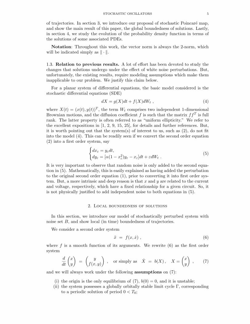
Definition 2. Let p be a point on Γ and S be a local cross section at p: a smooth1-dimensional arc, intersecting Γ (only) at p, transversally. Given an open andconnected neighborhood U of p, U ⊂ S, for every point u ∈ U , define the first returntime τ(u) as

τ(u) = inf{t > 0 : φt(u) ∈ S} .Then, the Poincare map P : U → S is defined by

P (u) = φτ(u)(u) , u ∈ U .

SP(u)

u

Figure 2. Poincare map

Clearly P (p) = p and τ(p) = T0.

With the help of the above definition, we can finally clarify assumption (ii), thatwe made in Section 2 relative to system (7). We say that Γ is attractive, with rateα0, 0 < α0 < 1, if:

‖P (u)− p‖ ≤ α0‖u− p‖ , for all u ∈ U . (12)

As before, in case (7) depends on parameters, it has to be understood that theinequality α0 < 1 must hold uniformly with respect to parameters variation.

3.2. Stochastic Poincare map. Consider now the general SDE associated to (11):

dXε(t) = b(Xε(t))dt+ ε

(0

Wt(ω0)

), Xε(0) = u, (13)

where Xε(·), u ∈ R2 and Wt is a standard Wiener process in R1. In this case, it isknown (see [22]) that a unique strong solution exists locally, that is for times beforethe stochastic solution blows up to infinity.

If we try to define a (stochastic) Poincare map for (13), we face some intrinsicchallenges.


(1) With nonzero probability, the stochastic trajectory will not return “after oneloop” to a given section, even though the unperturbed trajectory is periodic.

(2) Even if the stochastic trajectory returns to a given section, the first returnpoint doesn’t represent all return points to that section. In fact, the trajec-tory can intersect a given section several times, even infinitely many times.[There is no monotonicity of motion with respect to a given section].

Selecting random perturbations from B in (3), and relative to the model (8),allows us to solve the above difficulties. In fact, the following two facts hold as aconsequence of Theorem 1 and of (the proof of) Theorem 4 below.

(1) First, for all events in B, the stochastic trajectory of(8) will return to a givensection.

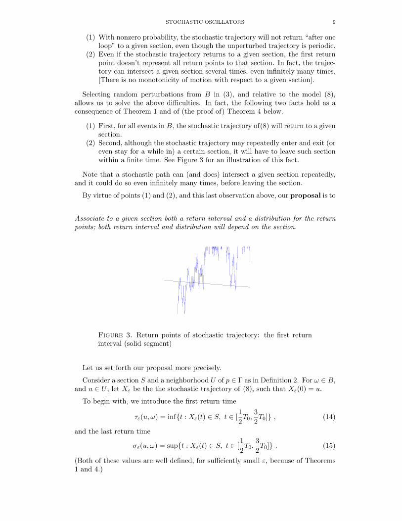
(2) Second, although the stochastic trajectory may repeatedly enter and exit (oreven stay for a while in) a certain section, it will have to leave such sectionwithin a finite time. See Figure 3 for an illustration of this fact.

Note that a stochastic path can (and does) intersect a given section repeatedly,and it could do so even infinitely many times, before leaving the section.

By virtue of points (1) and (2), and this last observation above, our proposal is to

Associate to a given section both a return interval and a distribution for the returnpoints; both return interval and distribution will depend on the section.

Figure 3. Return points of stochastic trajectory: the first returninterval (solid segment)

Let us set forth our proposal more precisely.

Consider a section S and a neighborhood U of p ∈ Γ as in Definition 2. For ω ∈ B,and u ∈ U , let Xε be the the stochastic trajectory of (8), such that Xε(0) = u.

To begin with, we introduce the first return time

τε(u, ω) = inf{t : Xε(t) ∈ S, t ∈ [1

2T0,

3

2T0]} , (14)

and the last return time

σε(u, ω) = sup{t : Xε(t) ∈ S, t ∈ [1

2T0,

3

2T0]} . (15)

(Both of these values are well defined, for sufficiently small ε, because of Theorems1 and 4.)


Then, we define the return “interval” E(u, ω) or simply E:

E = {Xε(t) : Xε(t) ∈ S, t ∈ [τε, σε]} . (16)

(Again, Theorems 1 and 4 ensure that E is well defined.)

Our proposal is to associate to E in (16) a “ return distribution” function Pu,ω,by which we can solve for the sample average of the set E. Since the distributionconveys all information on the return points, the Poincare map (call it Pε) shouldbe constructed as a point-to-distribution map, for each stochastic path:

Pε : u ∈ U → Pu,ω .

At the same time, from the foregoing, it is natural to define three different point-to-point maps, all of which can be computed in a numerical simulation: first returnmap, last return map and average return map.

Definition 3. Let the cross section S, neighborhood U , and Poincare map P , bedefined as in Definition 2, for the unperturbed system (7).

Let ω ∈ B, and Xε be the solution of (8). Then, we define stochastic Poincaremaps Pε, Pε : U → S, as follows.

• For ε = 0, P0 = P .• For ε 6= 0, and any u ∈ U , then we define:

– the first return map

Pε(u, ω) = Xε(τε(u, ω)) , (17)

where τε is defined in (14);– the last return map

Pε(u, ω) = Xε(σε(u, ω)) , (18)

where σε is defined in (15);– and the average return map

Pε(u, ω) =

∫EydPu,ω(y) , (19)

where E is defined in (16) and Pu,ω is the return distribution functionassociated to E.

Remark 1. In the recent work [14], the authors proposed a Poincare map definitionfor the van der Pol oscillator, subject to standard white noise perturbation on εdWt.Assuming that trajectories return to a given section (although there is a positiveprobability that they will not return), the authors further looked at the first returnmap and for sufficient small ε, argued that this map can be viewed as a Gaussianperturbation of the deterministic map. By comparison, restricting to noise fromwithin B, we actually proved that trajectories always return (for ε sufficiently small)to a given section. Furthermore, our proposal of Poincare map takes into accountall return points, and it gives a more detailed description relative to a given section,description which is not availably by a simple Gaussian process.

3.3. Global boundedness. By exploiting the Poincare map, we will show our maintheorem, which we state next.

Theorem 4. Consider the system (8), where ω is in B defined by (3). Assume that(12) holds, and that the assumptions of Lemmata 5 and 6 below hold (in particular,


(24)). Then, for ε > 0 sufficiently small, the stochastic trajectories of (8) areglobally bounded:

supt≥0‖Xε(t, ω)‖ <∞ .

To prove this result, we will proceed according to the following steps.

(1) We define the Poincare section S as a line section, and show closeness be-tween unperturbed and stochastic solutions during the first return time; seeLemma 5.

(2) We construct the first return map Pε (see Definition 3), and sharpen theresult of Lemma 5 about closeness of the stochastic trajectory and the un-perturbed Poincare map for the first return to the given section; see Lemma6.

(3) Combining the above closeness results, and asymptotic stability of the deter-ministic limit cycle, we show that there exists a neighborhood (an interval) Uεof p ∈ Γ, Uε ⊂ S, invariant under the stochastic Poincare map: Pε(Uε) ⊂ Uε.This will complete the proof.

First of all, we define the Poincare section. Through the polar representationof points in the plane, we take the section to be a line segment placed at a givenangular value θ0:

S = {(x, y) ∈ R2 : x = r(θ0) cos(θ0) , y = r(θ0) sin(θ0)} , (20)

where a(θ0) ≤ r(θ0) ≤ b(θ0), and a and b are chosen sufficiently small so that the linesegment S intersects Γ transversally at just one point. With this, we can identifypoints of the stochastic trajectory that returns to this section:

θε(t) = θε(0) = θ0 .

Naturally, the neighborhood U ⊂ S as in Definition 3, now becomes an open subin-terval of S containing the intersection with Γ. This way of proceeding will bevalidated in Lemma 5.

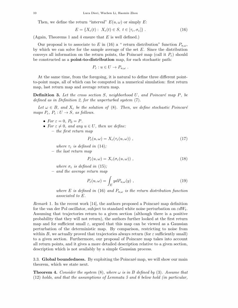
To illustrate, in Figure 4, we show a typical stochastic trajectory of (2) startingfrom the section S, and traveling around the origin once before returning to S.

Detail at section

Figure 4. One realization for the stochastic van der Pol oscillator:on the section are all return points


With this, we can be more specific about the meaning of first return time withrespect to the section (cfr. with (17)):

τ1ε = inf{t : θε(t) = θε(0)− 2π} . (21)

Without loss of generality, here below we will also make a simplification in thedefinition of B:“we require T = 2T0 in (3), where T0 > 0 is the period of the periodic solution of(7)”.This choice is legitimate, since we can always modify M to ensure that Theorem 1holds for T = 2T0. So, to reiterate, the event set B is henceforth given by

B = { ω : sup|t−s|≤T

|Wt(ω)−Ws(ω)| ≤M , and T = 2T0} . (22)

Finally, let L be the local Lipschitz constant of b(X) in (7) for ‖X‖ ≤ sup0≤t≤T ‖Xε(t, ω)‖.

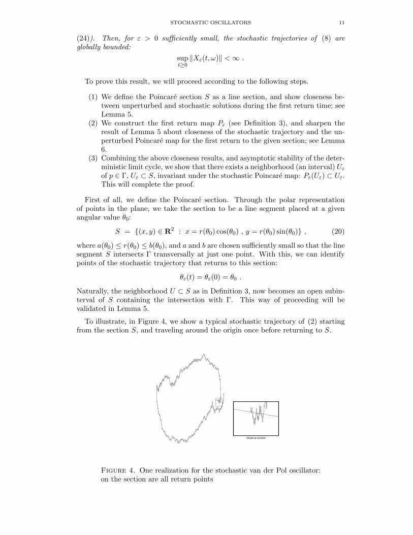
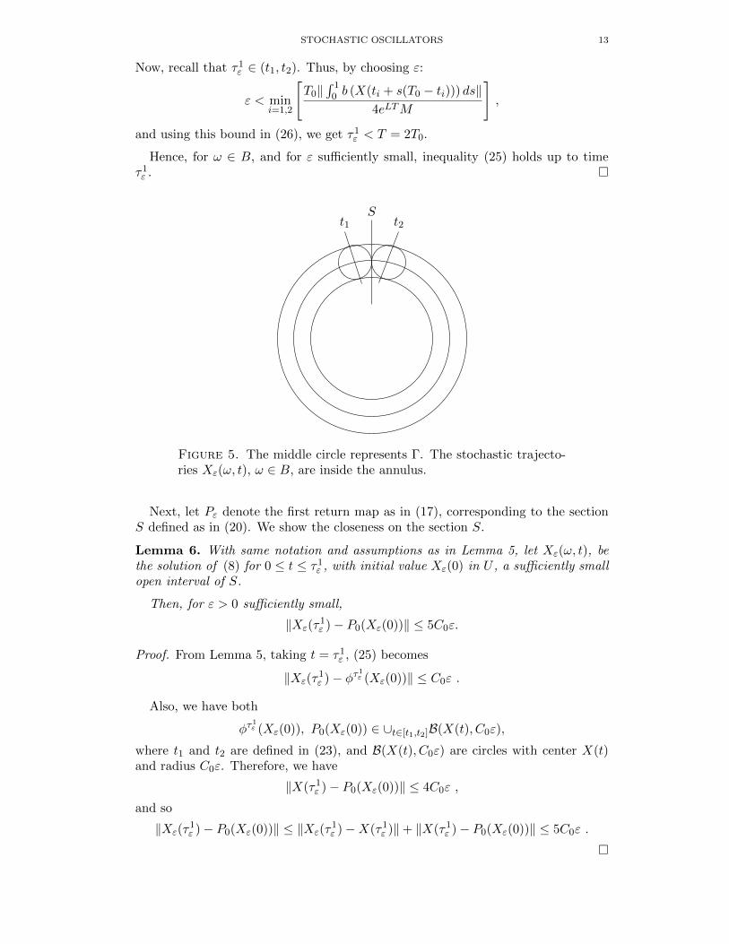
We further consider the annular neighborhood of radius εeLTM around the peri-odic trajectory Γ; see Figure 5. Finally, we let times t1 and t2 be defined as follows(again, see Figure 5):

t1 = inf{t > 1

2T0 : ‖X(t)−X(T0)‖ = εeLTM} ,

t2 = sup{t < 3

2T0 : ‖X(t)−X(T0)‖ = εeLTM} .

(23)

Note that t1, t2 depend on ε, and that by continuity of the strong solution Xε(t),τ1ε ∈ (t1, t2). Also, note that for ε > 0 sufficiently small, with t1, t2 as in (23), then

for i = 1, 2, we have: ∫ 1

0b (X(ti + s(T0 − ti))) ds 6= 0 . (24)

We are now ready to show closeness after the first return time.

Lemma 5. Let B be as in (22), ω ∈ B, and let L, T0, and τ1ε be as above. Then,

for ε > 0 sufficiently small, we have:

τ1ε < 2T0 ,

and

sup0≤t≤τ1ε

‖Xε(t, ω)−X(t)‖ < C0ε ,

where C0 = eLTM .

Proof. Proceeding as in the derivation of (10), we have

sup0≤s≤T

‖Xε(s)−X(s)‖ ≤ εeLTM . (25)

Consider the deterministic system (7). For either i = 1 or i = 2, we have

X(T0)−X(ti) =

∫ T0

ti

b(X(s))ds =

∫ 1

0b (X(ti + s(T0 − ti))) ds (T0 − ti) .

Since (24) holds, we can solve for |T0 − ti| from this last equation:

|T0 − ti| =‖X(T0)−X(ti)‖

‖∫ 1

0 b (X(ti + s(T0 − ti))) ds‖. (26)


Now, recall that τ1ε ∈ (t1, t2). Thus, by choosing ε:

ε < mini=1,2

[T0‖

∫ 10 b (X(ti + s(T0 − ti))) ds‖

4eLTM

],

and using this bound in (26), we get τ1ε < T = 2T0.

Hence, for ω ∈ B, and for ε sufficiently small, inequality (25) holds up to timeτ1ε . �

St2t1

Figure 5. The middle circle represents Γ. The stochastic trajecto-ries Xε(ω, t), ω ∈ B, are inside the annulus.

Next, let Pε denote the first return map as in (17), corresponding to the sectionS defined as in (20). We show the closeness on the section S.

Lemma 6. With same notation and assumptions as in Lemma 5, let Xε(ω, t), bethe solution of (8) for 0 ≤ t ≤ τ1

ε , with initial value Xε(0) in U , a sufficiently smallopen interval of S.

Then, for ε > 0 sufficiently small,

‖Xε(τ1ε )− P0(Xε(0))‖ ≤ 5C0ε.

Proof. From Lemma 5, taking t = τ1ε , (25) becomes

‖Xε(τ1ε )− φτ1ε (Xε(0))‖ ≤ C0ε .

Also, we have both

φτ1ε (Xε(0)), P0(Xε(0)) ∈ ∪t∈[t1,t2]B(X(t), C0ε),

where t1 and t2 are defined in (23), and B(X(t), C0ε) are circles with center X(t)and radius C0ε. Therefore, we have

‖X(τ1ε )− P0(Xε(0))‖ ≤ 4C0ε ,

and so

‖Xε(τ1ε )− P0(Xε(0))‖ ≤ ‖Xε(τ

1ε )−X(τ1

ε )‖+ ‖X(τ1ε )− P0(Xε(0))‖ ≤ 5C0ε .

�


Finally, we show global boundedness and complete the proof of Theorem 4, byusing the stability of the deterministic limit cycle, as epxressed by (12), and localboundedness of Xε.

In the proof below, we will need to compare the stochastic and deterministicsolutions. For this reason, we will use the following notation. For all k = 1, 2, . . . ,we write

φ∆kε

(Xε

( k∑i=1

τ iε

)), where ∆k

ε := τk+1ε − τkε ,

for the solution of the deterministic equation (7) at time τk+1ε , which started at time

τkε with initial condition Xε(∑k

i=1 τiε). Above, we have recursively defined the values

τkε as the k-th “first return” times:

τkε = inf{t > τk−1ε : θε(t) = θε(0)− 2π} , k = 1, 2, . . . , τ0

ε = 0 . (27)

These values τkε will be shown to be well defined in the proof below.

Proof of Theorem 4. First, let us show that

supk‖Xε(

k∑i=1

τ iε)‖ <∞ ,

by showing that there exists an interval Uε ⊂ S,

Uε = {X : ‖X − p‖ ≤ R0} , such that Pε(Uε) ⊂ Uε .

We show this last fact by induction, in the process showing that the times τkε ’s arewell defined.

If k = 1, from Lemma 5, τ1ε exists, and τ1

ε ∈ (t1, t2) with t1 and t2 given in (23),in particular τ1

ε ∈ (12T0,

32T0). From Lemma 6, we have

‖Xε(τ1ε )− P0(Xε(0))‖ ≤ R1ε ,

where R1 = 5C0, and C0 = eLTM with L the Lipschitz constant of b for X: ‖X‖ ≤sup0≤t≤2T0 ‖Xε(t, ω)‖.

Also, since Xε(0) ∈ Uε, denoting with p ∈ S the fixed point of P0 and using (12),we have

‖Xε(τ1ε )− p‖ ≤ ‖Xε(τ

1ε )− P0(Xε(0))‖+ ‖P0(Xε(0))− p‖

≤ R1ε+ α0R0 .

So, if ε < (1−α0)R0

R1, then Xε(τ

1ε ) ∈ Uε.

By induction, suppose that for j = 1, . . . , N , the times τ jε are well defined, thatsatisfy

τj−1 +1

2T0 ≤ τ jε ≤ τj−1 +

3

2T0 ,

where we have set

τj−1 :=

j−1∑i=0

τ iε ,

and that

‖Xε(τN )− p‖ ≤N−1∑k=0

αk0R1ε+ α0R0 .


Note that, since 0 < α0 < 1, then∑N−1

k=0 αk0 ≤∑∞

k=0 αk0 = 1

1−α0. Therefore, choosing

ε < (1−α0)2R0

R1will give X(τN ) ∈ Uε.

Now, when k = N + 1, consider equation (7) with initial condition Xε(τN ). ByGronwall inequality, we have

supτN≤s≤τN+T

‖Xε(s)− φ∆Nε

(Xε(τN )

)‖ ≤ C0ε,

hence τN + 12T0 < τN+1

ε < τN + 32T0. Also, since

‖Xε(τN+1)− φ∆Nε

(Xε(τN )

)‖ ≤ C0ε ,

similarly to the proof of Lemma 6, then

‖Xε(τN+1ε )− P0(Xε(τ

Nε ))‖ ≤ R1ε . (28)

Using contractility of the Poincare map as expressed by (12), and Xε(τNε ) ∈ Uε, we

have

‖P0(Xε(τNε ))− p‖ ≤ α0‖Xε(τ

Nε )− p‖ . (29)

Combining inequalities (28) and (29), we obtain

‖Xε(τN+1ε )− p‖ ≤‖Xε(τ

N+1ε )− P0(Xε(τ

Nε ))‖+ ‖P0(Xε(τ

Nε ))− p‖

≤R1ε+ α0‖Xε(τNε )− p‖ ≤

N∑k=0

αk0R1ε+ α0R0 .

In particular, if ε < (1−α0)2R0

R1, then X(τN+1) ∈ Uε, and this completes the induction

process.

Finally, since for all k, τk−1 + 12T0 < τkε < τk−1 + 3

2T0, then τkε must be in betweentwo consecutive multiples of the period T0. As a consequence of this, for any time twe can write t = τkε + s, for some k, and with 0 ≤ s ≤ T0. Using again Theorem 1,we then obtain

supt≥0‖Xε(t)‖ <∞ ,

which completes the proof. �

Remark 2. The main implication of Theorem 4 is that, although random perturba-tion in B will not be bounded for all times, the stochastic trajectories will remainwithin a tubular neighborhood of the deterministic limit cycle.

Remark 3. To illustrate the situation, consider a system (7) which is unambiguouslyrepresentable in polar coordinates (for example, the van der Pol oscillator), usepolar coordinates (ρ, θ) for the deterministic problem, and (ρε(t), θε(t)) to modelamplitude and phase in the stochastically perturbed version. Theorem 4 impliesthat -as long as the perturbation is selected from within the set B– the amplitudeρε remains bounded:

supt≥0, ω∈B

|ρε(t)− ρ(t)| <∞ .

In turns, this helps explaining why we observe no catastrophic breakdown in cell-phone service, in agreement with practical experience.

At the same time, we must emphasize that the phase perturbation does becomeunbounded:

supt≥0, ω∈B

|θε(t)− θ(t)| =∞ .


In turns, this helps explaining why we may (and do) lose cell phone connectionduring lengthy conversations; see details in [6].

To sum up, although perturbations occur in both amplitude and phase, there isa clear distinction among the two: in particular, the strong stability property of thedeterministic limit cycle ensures that the amplitude perturbations remain bounded.

4. Connection with Partial differential equations

In this section, we attempt deriving PDEs for the transition density functionassociated to the trajectories of (8), with ω ∈ B. First, we review some knownresults and give needed notations.

4.1. Diffusion process and partial differential equations. For completeness,here we review the standard derivation of PDEs for diffusion processes; for details,see [22].

Consider a d-dimensional Markov family {Xt,Ft}, which is a diffusion processwith drift vector b = (b1, . . . , bd) and diffusion matrix a = {aik}1≤i,k≤d.

This means that for any f ∈ C2, one has

limt→0

1

t[E f(Xt|X0 = x)− f(x)] = (Lf)(x), ∀x ∈ Rd ,

where the infinitesimal operator L is given by

(Lf)(x) =1

2

d∑i=1

d∑k=1

aik(x)∂2f(x)

∂xi∂xk+

d∑i=1

bi(x)∂f(x)

∂xi.

Suppose that the Markov family of Xt has a transition density function

P (Xt ∈ dy|X0 = x) = p(t, x, y)dy; ∀x ∈ Rd , t > 0 .

Then, p(t, x, y) satisfies the forward Kolmogorov (Fokker-Planck) equation, for fixedx ∈ Rd:

pt(t, x, y) = L∗p(t, x, y); (t, y) ∈ (0,∞)×Rd ,

and the backward Kolmogorov equation, for fixed y ∈ Rd:

pt(t, x, y) = Lp(t, x, y); (t, x) ∈ (0,∞)×Rd ,

where the adjoint operator L∗ is given by

(L∗f)(x) =1

2

d∑i=1

d∑k=1

∂2(aik(x)f(x))

∂xi∂xk−

d∑i=1

∂(bi(x)f(x))

∂xi, ∀x ∈ Rd .

4.2. Killed diffusions. Let us also introduce the killed diffusion PDE, by consid-ering the one dimensional diffusion process

dXt = b(Xt)dt+ σ(Xt)dWt, X0 = x , (30)

where b, σ are Lipschitz functions, and Wt is a standard Wiener process. Considerevents set C:

C = {ω : sup0≤s≤t

|Xs| ≤M0} .

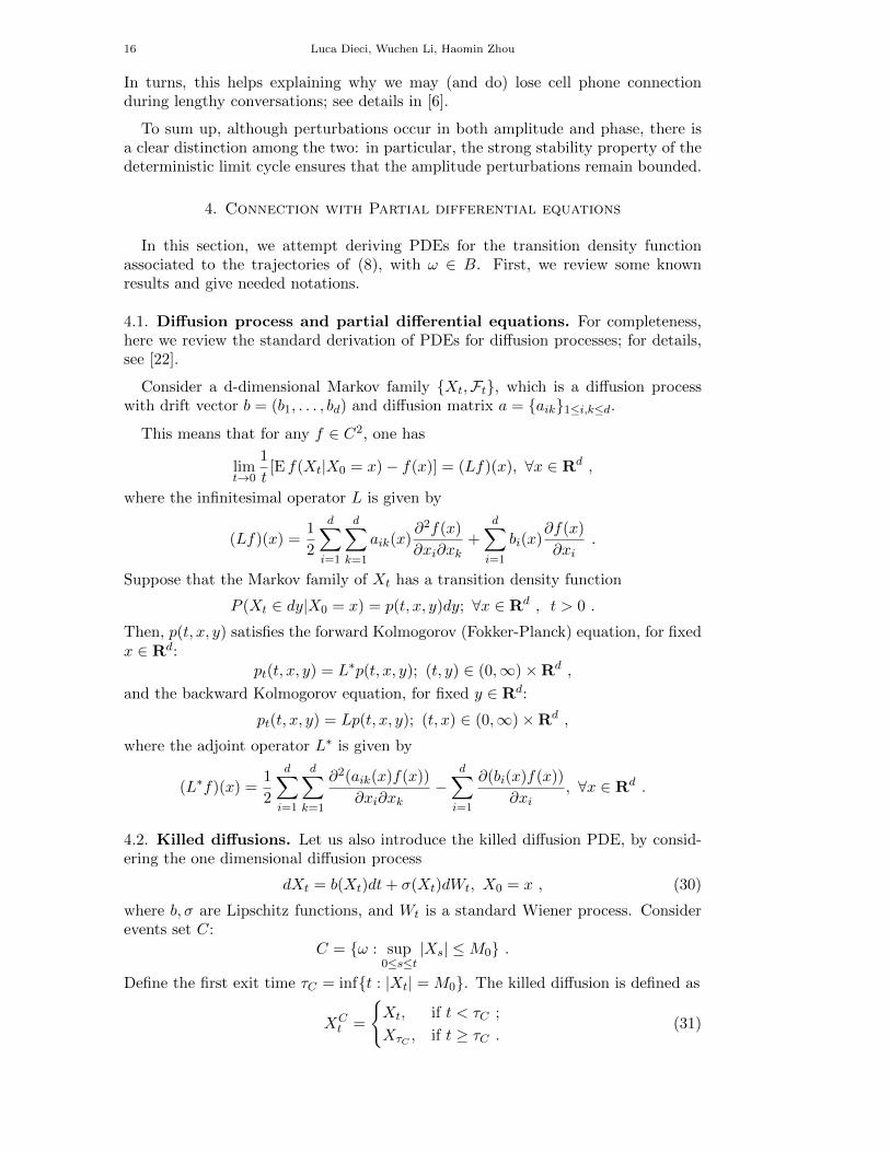
Define the first exit time τC = inf{t : |Xt| = M0}. The killed diffusion is defined as

XCt =

{Xt, if t < τC ;

XτC , if t ≥ τC .(31)


(a) XτC = M0 (b) XτC = −M0

Figure 6. Killed diffusion

Consider the transition density function p(t, x, y) of XCt :

p(t, x, y)dy = P (XCt ∈ dy|X0 = x) .

In Lemma 7, we give the Fokker-Planck equation for the killed diffusion XCt ,

which is a PDE with vanishing boundary conditions on a finite interval. For theproof of Lemma 7, we refer to [13] and [24].

Lemma 7. For fixed x, p(t, x, y) solvespt = −(bp)y + 1

2(σ2p)yy , |y| < M0 ,

p(t, x, y) = 0, |y| = M0 ,

p(0, x, y) = δ0(x− y) .

�

4.3. Derivation of PDE. However, there are difficulties in following the abovestandard steps to derive the evolution conditioned on B, because:

• Xε(t) is not a Markov process, since it depends both on values in the pastand in the future; in fact, Xε(t) depends on the full set of values in the timeinterval (t− T, t+ T ).

Because of the above difficulty, we restrict to a subset of B which allows us torestart the process at certain times, and which is more amenable to analysis. As in(22), take T = 2T0, where T0 is the period of the deterministic limit cycle. Then,we consider the events set

B0 = {ω : sup0≤t≤T0

|Wt+kT0 −WkT0 | ≤1

2M} . (32)

Clearly, B0 in (32) is a subset of B in (22). With respect to B, B0 has the advantagethat, on each time interval of width T0, the Wiener process increments are indepen-dent of that previous time interval of width T0. Moreover, for first time interval, byintroducing the absolute running maximum

Mt = sup0≤s≤t

|Wt| , t ≤ T0 ,

(Xε(t),Wt,Mt) forms a Markov process, since condition B0 is nothing but the re-striction to those events for which Mt is bounded.


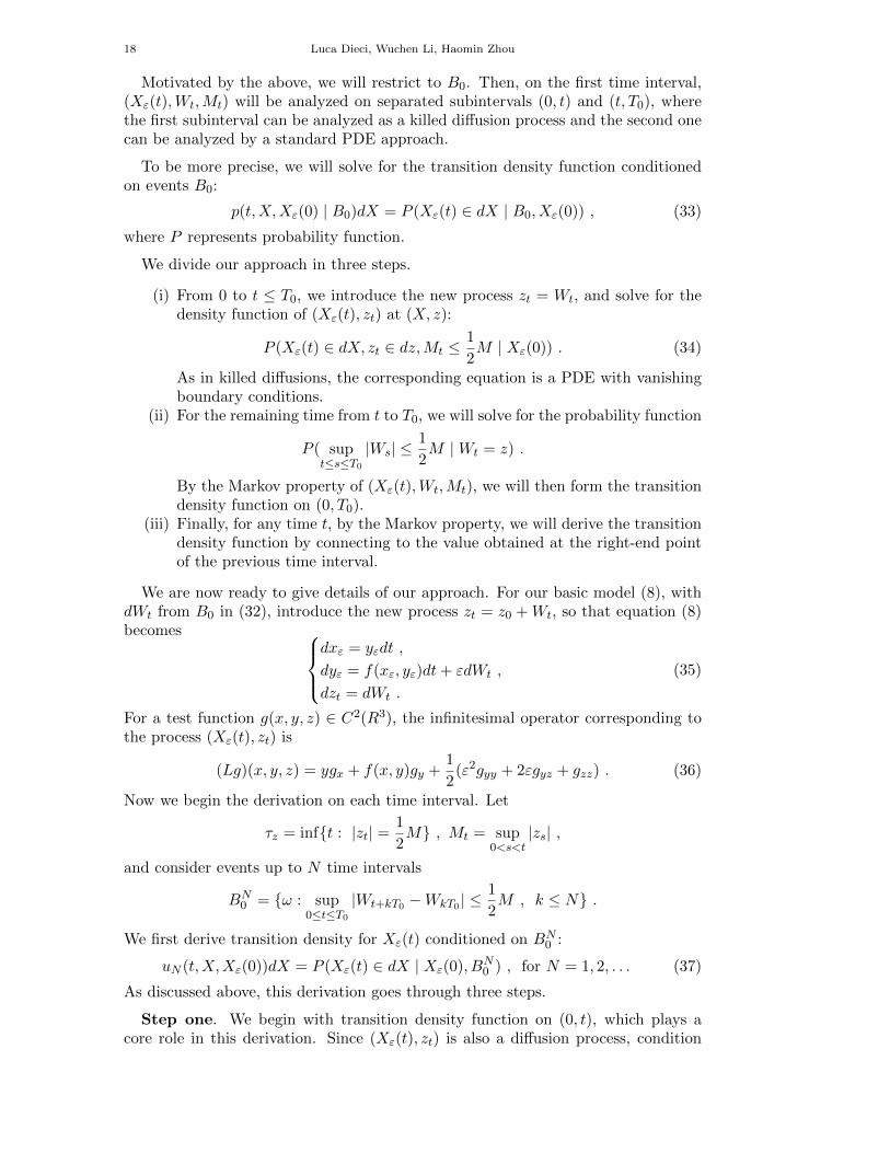
Motivated by the above, we will restrict to B0. Then, on the first time interval,(Xε(t),Wt,Mt) will be analyzed on separated subintervals (0, t) and (t, T0), wherethe first subinterval can be analyzed as a killed diffusion process and the second onecan be analyzed by a standard PDE approach.

To be more precise, we will solve for the transition density function conditionedon events B0:

p(t,X,Xε(0) | B0)dX = P (Xε(t) ∈ dX | B0, Xε(0)) , (33)

where P represents probability function.

We divide our approach in three steps.

(i) From 0 to t ≤ T0, we introduce the new process zt = Wt, and solve for thedensity function of (Xε(t), zt) at (X, z):

P (Xε(t) ∈ dX, zt ∈ dz,Mt ≤1

2M | Xε(0)) . (34)

As in killed diffusions, the corresponding equation is a PDE with vanishingboundary conditions.

(ii) For the remaining time from t to T0, we will solve for the probability function

P ( supt≤s≤T0

|Ws| ≤1

2M |Wt = z) .

By the Markov property of (Xε(t),Wt,Mt), we will then form the transitiondensity function on (0, T0).

(iii) Finally, for any time t, by the Markov property, we will derive the transitiondensity function by connecting to the value obtained at the right-end pointof the previous time interval.

We are now ready to give details of our approach. For our basic model (8), withdWt from B0 in (32), introduce the new process zt = z0 +Wt, so that equation (8)becomes

dxε = yεdt ,

dyε = f(xε, yε)dt+ εdWt ,

dzt = dWt .

(35)

For a test function g(x, y, z) ∈ C2(R3), the infinitesimal operator corresponding tothe process (Xε(t), zt) is

(Lg)(x, y, z) = ygx + f(x, y)gy +1

2(ε2gyy + 2εgyz + gzz) . (36)

Now we begin the derivation on each time interval. Let

τz = inf{t : |zt| =1

2M} , Mt = sup

0<s<t|zs| ,

and consider events up to N time intervals

BN0 = {ω : sup

0≤t≤T0|Wt+kT0 −WkT0 | ≤

1

2M , k ≤ N} .

We first derive transition density for Xε(t) conditioned on BN0 :

uN (t,X,Xε(0))dX = P (Xε(t) ∈ dX | Xε(0), BN0 ) , for N = 1, 2, . . . (37)

As discussed above, this derivation goes through three steps.

Step one. We begin with transition density function on (0, t), which plays acore role in this derivation. Since (Xε(t), zt) is also a diffusion process, condition


transition density for (Xε(t), zt) with event {Mt ≤ 12M} is the same as a killed

diffusion process, where we only cut off on the zt part. To be more precisely, wedefine following killed diffusion by

(XMε (t), zMt ) =

{(Xε(t), zt), if t < τz ;

(Xε(τz), zτz), if t ≥ τz .(38)

The transition density of (XMε (t), zMt ) is the same as (34).

In details, consider B10 . For τz > t and fixed Xε(0), we derive the transition

density function u of process (Xε(t), zt) with events {Mt ≤ 12M}:

u(t,X, z,Xε(0))dXdz =P (Xε(t) ∈ dX, zt ∈ dz,Mt ≤1

2M | Xε(0), z0 = 0)

=P (XMε (t) ∈ dX, zMt ∈ dz | Xε(0), z0 = 0) .

For fixed (Xε(0), z0), we also denote u(t,X, z,Xε) = u(t,X, z). The correspondingFokker-Planck equation becomes

∂u∂t = L∗u, (X, z) ∈ D ,

u(t,X, z) = 0, |z| = 12M ,

u(0, X, z) = δ(0,0,0)(X − (xε(0), yε(0)), z − z0) ,

(39)

where

D = R×R× (−1

2M,

1

2M) .

Remark 4. This degenerate equation is similar to that in [21].

We delay justification of equation (39) until the end.

Step two. Here we discuss the event on (t, T0). At time t, restricting to theevents in B1

0 is equivalent to requiring that the process zt remains bounded up totime T0.

Consider the probability of zt remaining bounded until time t while starting atpoint z:

v(t, z) = P (τz > t | z0 = z) .

Here v represents probability of the events {sup0≤s≤t |Ws + z| ≤ 12M}. Then (see

[22]), v(t, z) satisfies the following PDE:vt = 1

2vzz, −12M < z < 1

2M , t > 0 ,

v(t, 12M) = v(t,−1

2M) = 0 , t > 0 ,

v(0, z) = 1, −12M < z < 1

2M .

(40)

Here, (40) can be solved. The remaining probability becomes

v(T0 − t, z) = P ( supt≤s≤T0

|Ws| ≤1

2M |Wt = z) ,

and probability of B10 is

v(T0, 0) = P (B10) .

Combining step one and two: Since (Xε(t), zt,Mt) forms a Markov process, weobtain the joint transition density function for (Xε(t), zt) with B1

0 :

p(t,X, z,Xε(0), B10)dXdz = P (Xε(t) ∈ dX, zt ∈ dz,B1

0 | Xε(0), z0 = 0) ,


which satisfies

p(t,X, z,Xε(0), B10) = u(t,X, z)P ( sup

t≤s≤T0|Ws| ≤

1

2M |Wt = z) .

And the marginal density becomes

p(t,X,Xε(0), B10) =

∫ 12M

− 12Mp(t,X, z,Xε(0), B1

0)dz .

The derivation becomes as following: for the first time interval (0, T0), recall u1

defined in (37) represents transition density function for Xε(t) conditioned on B10 ,

which statisfies

u1(t,X,Xε(0)) =p(t,X,Xε(0), B1

0)

P (B10)

=

∫ 12M

−12M

u(t,X, z)v(T0 − t, z)dz

v(T0, 0),

where u satisfies equation (39) with Xε(0), z0 = 0 and v is the solution of equation(40).

Step three. “Refreshing”. Xt under B0 can be seen as a refreshed process at eachtime kT0. And by applying the Markov property, we can derive general transitiondensity function for Xε(t).

Consider the events set BN+10 . We denote w as the transition density function for

(Xε(t), zt) with events Bt:

w(t,X, z,Xε(0), z0)dXdz = P (Xε(t) ∈ dX, z(t) ∈ dz,Bt | Xε(0), z0) ,

where

Bt = {ω : sup0<s<T0s+kT0≤t

|Ws+kT0 −WkT0 | ≤M} .

Again, for fixed X0, we denote w = w(t,X, z), and by Chapman−Kolmogorov equa-tion

w(t,X, z) =

∫R2

. . .

∫R2

u(t, X, XN )

N−1∏i=0

u(T0, Xi+1, Xi)dX1dX2 . . . dXN ,

where we used the notation Xi = (Xi, zi), and X0 = (Xε(0), 0). Combining eventsfrom time t to (N + 1)T0, we have

uN+1(t,X,Xε(0)) =

∫ 12M

− 12Mw(t,X, z)v((N + 1)T0 − t, z)dz

P (BN+10 )

=

∫ 12M

− 12Mw(t,X, z)v((N + 1)T0 − t, z)dz

v(T0, 0)N+1.

Arbitrary t. From the independent increments property of B0 for each time in-terval, we can derive the transition density function for Xε(t) conditioned on B0.Indeed, for any t, there exists N = 0, 1, . . . , such that t ∈ [NT0, (N + 1)T0]. Then,we simply have

p(t,X,Xε(0) | B0) = uN+1(t,X,Xε(0)) .

Finally, we justfy equation (39).


Proof of (39). The basic approach we use is standard; e.g., see [13] and [23].

The boundary conditions can be given as u(0, x, y, z) = δ(0,0,0)(x − xε(0), y −yε(0), z − z(0)) and u(t, x, y,±1

2M) = 0. Next, we follow the same steps used toderive the Fokker-Planck equation for the diffusion process.

To simplify notation, denote Y = (x, y, z) and Yt = (xε(t), yε(t), z(t)). Considerany test function h(x, y, z) = h(Y ) ∈ C2 with compact support. Then,∫

Dh(Y )

∂u(t, Y )

∂tdY =

∫Dh(Y ) lim

∆t→0

u(t+ ∆t, Y )− u(t, Y )

∆tdY , (41)

where D = R×R×(−12M, 1

2M). Again, consider the process (Yt,Mt). Since (Yt,Mt)is a Markov process, if we denote its density function with p, which is defined by

p(t, Y, Y (0))dY = P (Yt ∈ dY,Mt ≤1

2M |Y (0)) ,

Therefore the Chapman−Kolmogorov equation implies

u(t+ ∆t, Y ) =p(t+ ∆t, Y, Y (0))

=

∫Du(t, Z)p(∆t, Y, Z)dZ .

Above, the last equality comes from the Markov property. Hence, equation (41)becomes ∫

Dh(Y )

∂u(t, Y )

∂tdY

=

∫Dh(Y ) lim

∆t→0

∫D u(t, Z)p(∆t, Y, Z)dZ − u(t, Y )

∆tdY

= lim∆t→0

∫D

∫D h(Y )u(t, Z)p(∆t, Y, Z)dZdY −

∫D h(Y )u(t, Y )dY

∆t

= lim∆t→0

∫D

∫D h(Y )u(t, Z)p(∆t, Y, Z)dY dZ −

∫D h(Z)u(t, Z)dZ

∆t

=

∫D

lim∆t→0

∫D h(Y )p(∆t, Y, Z)dY − h(Z)

∆tu(t, Z)dZ .

(42)

where the second and last equalities are justified by the dominated convergencetheorem, and the third equality comes from Fubini’s theorem. Since E(1{τz≤∆t}) =o(∆t) and h is a bounded function, then

lim∆t→0

∫D h(Y )p(∆t, Y, Z)dY − h(Z)

∆t= lim

∆t→0

Eh(Y∆t)1{τz>∆t} − h(Z)

∆t

= lim∆t→0

[Eh(Y∆t)− h(Z)

∆t−

Eh(Y∆t)1{τz≤∆t}

∆t] = Lh(Z) ,

where L is the infinitesimal operator defined by (36). Hence (42) becomes∫Dh(Y )

∂u(t, Y )

∂tdy =

∫DLh(Z)u(t, Z)dZ .

Integrating by parts, using u(t, Z) = 0 on the boundary and letting Z = Y on theright-hand-side, we then obtain∫

Dh(Y )

∂u(t, Y )

∂tdY =

∫Dh(Y )L∗u(t, Y )dY ,

which gives the equation (39). �


5. Conclusions

In this work, motivated by practical observations (real world phenomena, labora-tory experiments, and numerical simulations) on typical engineering circuitries, wereconsidered what model of noise is appropriate for the mathematical modeling ofstochastic perturbation of second order systems of differential equations that admitstable limit cycles. Whereas classical models consider stochastic DEs where per-turbations come from standard Brownian motion paths, we restricted the class ofallowed disturbances, to avoid pumping infinite energy into the system through thenoise. In essence, our new model consists in selecting those Brownian paths thathave bounded increments in finite time.

Of course, there are new challenges when one gives up familiar ground, suchas white noise perturbations, and indeed we have encountered technical difficultiesespecially insofar as obtaining viable expression for the transition density function.However, by selecting the allowed perturbations from within our proposed eventset, we were able to adopt many classical tools from dynamical systems, and showsome interesting mathematical results, that further appear to be more in tune withpractically observed circuitry behaviors.

Relative to our set of allowed stochastic perturbations, our main results have beenthe following.

(i) We proved global boundedness of the stochastic trajectories, and we showedthat they remain (for small values of the parameter ε appearing in front ofthe perturbation term) in the neighborhood of the deterministic limit cycle.

(ii) We proposed, and ensured the existence, of stochastic Poincare map(s) asa point-to-distribution map, and further introduced three point-to-pointPoincare maps: first, last, and average return maps.

(iii) We associated the study of transition densities to a pair of PDEs.

In the future, we plan to further explore selected aspects of the present work.In particular, we plan to study (at least experimentally) the statistical propertiesof the return distribution associated to the Poincare map, and to further performnumerical exploration of the approach based on the system of PDEs herein derived.

References

[1] L. Arnold. Stochastic Differential Equations: Theory and Applications. John Wiley & Sons,1974.

[2] L. Arnold. Random Dynamical Systems, 2nd Edition. Springer-Verlag, Berlin, 2003.[3] Peter H Baxendale. Lyapunov exponents and stability for the stochastic Duffing-van der Pol

oscillator. IUTAM Symposium on Nonlinear Stochastic Dynamics, pages 125–135. Springer,2003.

[4] Peter H Baxendale. Stochastic averaging and asymptotic behavior of the stochastic Duffing–van der Pol equation. Stochastic Processes and Their Applications, 113(2):235–272, 2004.

[5] K.L. Chen, Z.Z. Sun, S. Yin, Y.Q. Wang, and X.R. Wang. Deformation of limit cycle underperturbations. Superlattices and microstructures. v. 37, (3), 2005, MAR, pp 185–191.

[6] Shui-Nee Chow and Hao-Min Zhou. An analysis of phase noise and Fokker–Planck equations.Journal of Differential Equations, 234(2):391–411, 2007.

[7] A. Demir, A. Mehrotra and J. Roychowdhury. Phase noise in oscillators: A unifying theoryand numerical methods for characterization. IEEE Trans. Circuits and Systems-I: FundamentalTheory and Applications, vol. 47, No. 5, May 2000, 655–674.

[8] Erturk, A. and D.J. Inman. Piezoelectric Energy Harvesting. Wiley. 2011.[9] Mark Freidlin and Alexander D Wentzell. Random perturbations of dynamical systems, Third

Edition, volume 260. Springer, 2012.


[10] P. Friz and M. Hairer. A course on rough paths. Springer, 2014.[11] A. Hajimiri, S. Limotyrakis and T. Lee. Jitter and phase noise in ring oscillators IEEE J.

Solid State Circuits, Vol. 34, No. 6, June 1999, 790–804.[12] Hale, Jack K., and Huseyin Kocak. Dynamics and bifurcations. Springer, 1991.[13] Henkel, Hartmuth. Range-based parameter estimation in diffusion models. Diss. Humboldt-

Universitt zu Berlin, Mathematisch-Naturwissenschaftliche Fakultat II, 2010.[14] Hitczenko, Pawel, and Georgi S. Medvedev. The Poincare map of randomly perturbed periodic

motion. Journal of Nonlinear Science 23.5 (2013): 835-861.[15] P. Kloeden and E Platen. Numerical Solution of Stochastic Differential Equations. Springer-

Verlag, 1999.[16] Brian Nguyen Limketkai. Oscillator modeling and phase noise. PhD thesis, University of Cal-

ifornia, Berkeley, 2004.[17] B. Razavi. A study of phase noise in CMOS oscillators. IEEE. J. Solid State Circuits, Vol 31,

No. 3, Mar. 1996, 331–343.[18] Klaus Reiner Schenk-Hoppe. Deterministic and stochastic Duffing-van der Pol oscillators are

non-explosive. Zeitschrift fur angewandte Mathematik und Physik ZAMP, 47(5):740–759, 1996.[19] Klaus Reiner Schenk-Hoppe. Random attractors-general properties, existence and applications

to stochastic bifurcation theory. Discrete and Continuous Dynamical Systems, 4:99–130, 1998.[20] KR Schenk-Hoppe. Bifurcation scenarios of the noisy Duffing-van der Pol oscillator. Nonlinear

dynamics, 11(3):255–274, 1996.[21] Shreve, Steven E, Stochastic calculus for finance II: Continuous-time models. Vol. 11. Springer,

2004.[22] SE Shreve and I Karatzas. Brownian motion and stochastic calculus. Newyork Berlin. Heidel-

berg. London Paris Tokyo, 1991.[23] D. W. Stroock. Partial Differential Equations for Probabilists. Cambridge Univ. Press, 2008.[24] Daniel W Stroock and SR Srinivasa Varadhan. Multidimensional diffussion processes. volume

233. Springer, 1979.[25] S. Varadhan. Large Deviations and Applications. Society for Industrial Mathematics, Philadel-

phia, PA, 1984.

School of Mathematics, Georgia Tech, Atlanta, GA 30332 U.S.A.

E-mail address: [email protected], [email protected], [email protected]

Documents

A NEW MODEL FOR REALISTIC RANDOM PERTURBATIONS …people.math.gatech.edu/~dieci/preps/DLZ-Theory.pdf · A NEW MODEL FOR REALISTIC RANDOM PERTURBATIONS OF STOCHASTIC OSCILLATORS LUCA