Embed Size (px)
Citation preview
Finite Rank Perturbations of Random Matricesand Their Continuum Limits
by
Alexander Bloemendal
A thesis submitted in conformity with the requirementsfor the degree of Doctor of PhilosophyGraduate Department of Mathematics
University of Toronto
Copyright c© 2011 by Alexander Bloemendal
Abstract
Finite Rank Perturbations of Random Matrices
and Their Continuum Limits
Alexander Bloemendal
Doctor of Philosophy
Graduate Department of Mathematics
University of Toronto
2011
We study Gaussian sample covariance matrices with population covariance a bounded-
rank perturbation of the identity, as well as Wigner matrices with bounded-rank additive
perturbations. The top eigenvalues are known to exhibit a phase transition in the large
size limit: with weak perturbations they follow Tracy-Widom statistics as in the un-
perturbed case, while above a threshold there are outliers with independent Gaussian
fluctuations. Baik, Ben Arous and Peche (2005) described the transition in the complex
case and conjectured a similar picture in the real case, the latter of most relevance to
high-dimensional data analysis.
Resolving the conjecture, we prove that in all cases the top eigenvalues have a limit
near the phase transition. Our starting point is the work of Ramirez, Rider and Virag
(2006) on the general beta random matrix soft edge. For rank one perturbations, a
modified tridiagonal form converges to the known random Schrodinger operator on the
half-line but with a boundary condition that depends on the perturbation. For general
finite-rank perturbations we develop a new band form; it converges to a limiting operator
with matrix-valued potential. The low-lying eigenvalues describe the limit, jointly as the
perturbation varies in a fixed subspace. Their laws are also characterized in terms of a
diffusion related to Dyson’s Brownian motion and in terms of a linear parabolic PDE.
We offer a related heuristic for the supercritical behaviour and rigorously treat the
ii

supercritical asymptotics of the ground state of the limiting operator.
In a further development, we use the PDE to make the first explicit connection be-
tween a general beta characterization and the celebrated Painleve representations of
Tracy and Widom (1993, 1996). In particular, for β = 2, 4 we give novel proofs of the
latter.
Finally, we report briefly on evidence suggesting that the PDE provides a stable, even
efficient method for numerical evaluation of the Tracy-Widom distributions, their general
beta analogues and the deformations discussed and introduced here.
This thesis is based in part on work to be published jointly with Balint Virag.
iii

Dedication
To my teachers, starting with my parents
iv

Acknowledgements
Without my wonderful thesis advisor Balint Virag, I would never have done any of
this work. Learning from and working with Balint has been a better experience than
anyone could hope for and I will say more about it presently.
I was fortunate to have my graduate work supported by an NSERC postgraduate
scholarship as well as departmental research assistantships. I also gained a great deal
from attending summer schools at PIMS and MSRI and workshops at CRM, MSRI and
AIM. I am further grateful to Alexei Borodin and the department at Caltech as well as
Balint Toth and the institute at the Technical University of Budapest for their hospitality
in the Spring and Fall of 2010.
Special thanks are due to Percy Deift, both for his careful and helpful comments on
this thesis and for making the trip to Toronto for my defense! I am also very appreciative
of Peter Forrester for his continued interest and encouragement, Alexander Its for his
patient and thorough explanations and Benedek Valko for discussions of drafts. I have
benefitted from interesting conversations with many others including Mark Adler, Jinho
Baik, Alexei Borodin, Iain Johnstone, Arno Kuijlaars, Pierre van Moerbeke, Eric Rains,
Brian Rider, Brian Sutton, Craig Tracy, Dong Wang, Harold Widom and Ofer Zeitouni.
Credit for the initial conception of certain ideas is shared with Jose Ramırez.
My professors at U of T have generously shared not only mathematics but guid-
ance over the years. I am especially grateful to Ed Bierstone, Jim Colliander, Michael
Goldstein, Kostya Khanin, Robert McCann, Mary Pugh, Joe Repka and Jeremy Quastel.
I am very happy to thank the departmental staff, but it is not possible to thank Ida
Bulat enough. I cannot remember all the times she went out of her way; I doubt I know
anyone else as patient, kind, dedicated or honestly as good at what they do.
Nor is it really possible to convey my appreciation for my family and friends. I am
very lucky to have these wonderful people in my life. To those who were closest to me
through the past few years: your company, support, empathy and humour helped me
more than you know. I couldn’t have done it without you.
Finally, I am forever indebted to Balint for things that went far beyond the call of
duty: for inspiring me out of my initial hesitation; for showing me so much beautiful
mathematics; for teaching me the value of thinking simply and expressing each thought
directly; for patiently encouraging me, always putting up with me, and never losing faith
even when I did. A true teacher, mentor, role model and friend, words do not express
the depth of my admiration and gratitude.
v
Contents
1 Introduction 1
1.1 Background . . . . . . . . . . . . . . . . . . . . . . . . . . . . . . . . . . 1
1.2 Contributions and outline . . . . . . . . . . . . . . . . . . . . . . . . . . 6
1.3 Concluding remarks . . . . . . . . . . . . . . . . . . . . . . . . . . . . . . 9
2 One spike 10
2.1 Introduction . . . . . . . . . . . . . . . . . . . . . . . . . . . . . . . . . . 10
2.2 Limits of spiked tridiagonal matrices . . . . . . . . . . . . . . . . . . . . 19
2.3 Application to Wishart and Gaussian models . . . . . . . . . . . . . . . . 31
2.4 Alternative characterizations of the laws . . . . . . . . . . . . . . . . . . 35
3 Several spikes 38
3.1 Introduction . . . . . . . . . . . . . . . . . . . . . . . . . . . . . . . . . . 38
3.2 A canonical form for perturbation in a fixed subspace . . . . . . . . . . . 46
3.3 Limits of block tridiagonal matrices . . . . . . . . . . . . . . . . . . . . . 52
3.4 CLT and tightness for Gaussian and Wishart models . . . . . . . . . . . 67
3.5 Alternative characterizations of the laws . . . . . . . . . . . . . . . . . . 74
4 Going supercritical 83
4.1 The supercritical end of the critical regime . . . . . . . . . . . . . . . . . 84
4.2 The limiting location . . . . . . . . . . . . . . . . . . . . . . . . . . . . . 89
vi
4.3 Heuristic for the limiting fluctuations . . . . . . . . . . . . . . . . . . . . 92
5 Connection with Painleve II 93
5.1 Tracy-Widom laws and rank one deformations . . . . . . . . . . . . . . . 94
5.2 Subsequent eigenvalue laws . . . . . . . . . . . . . . . . . . . . . . . . . . 98
5.3 Higher-rank deformations . . . . . . . . . . . . . . . . . . . . . . . . . . 100
6 A note on numerics 101
A Stochastic Airy is a classical Sturm-Liouville problem 105
Bibliography 111
vii
Chapter 1
Introduction
This introductory chapter briefly reviews some background material, sketches the contri-
butions of the thesis and provides an outline of subsequent chapters. Precise definitions
and statements as well as many additional references will be found in the opening sections
of the chapters, especially Chapters 2 and 3.
1.1 Background
Random matrices
Random matrix theory is predominantly concerned with the asymptotic spectral proper-
ties of large matrices with random entries jointly distributed according to one of several
natural models. Most classical are the Gaussian orthogonal, unitary and symplectic en-
sembles (GO/U/SE), introduced to physics by Wigner and Dyson in the 1950s and 60s.
These distributions on real symmetric, complex Hermitian or quaternion self-dual matri-
ces have density proportional to e−β4trA2
where β = 1, 2, 4 respectively; they are unique in
having the double virtue of invariance under the associated classical group of symmetries
as well as independence of the entries up to the algebraic constraints. They may also
be described by filling a matrix X with independent standard real/complex/quaternion
Gaussians and additively symmetrizing: A = 1√2(X + X†). General references include
Mehta (2004), Deift (1999), Anderson, Guionnet and Zeitouni (2009), Forrester (2010).
Already in the late 1920s, Wishart considered Gaussian sample covariance matrices.
Here one begins with a “data matrix” X of independent Gaussian columns and the
symmetrization is multiplicative: A = XX†. Wishart matrices continue to be of central
1
Chapter 1. Introduction 2
importance in multivariate statistics; see Muirhead (1982), Bai (1999), Anderson (2003).
There are several asymptotic regimes. At the global scale one may study the empirical
spectral distribution and find the famous Wigner semicircle and Marcenko-Pastur laws in
the Gaussian and Wishart cases respectively. The semicircle law states that, if λ1, . . . , λn
are the eigenvalues of an n× n GO/U/SE matrix, then with probability one there is the
weak convergence
1
n
n∑i=1
δλi/√n → µ where
dµ
dx=
√4− x22π
1[−2,2](x).
This law holds for much more general self-adjoint matrices with independent entries,
known as Wigner matrices.
Wigner and Dyson were originally intersted in eigenvalue spacing in the bulk of the
spectrum as a model for the excitation spectra of heavy nuclei. The setting of this thesis
is the point process formed by the largest eigenvalues, also referred to as the “soft edge”
of the spectrum. The fundamental limit law for the n×n GO/U/SE is due to Tracy and
Widom (1993, 1994, 1996); for the largest eigenvalue λ1 it states that
Pn
(n1/6
(λ1 − 2
√n)≤ x
)→ Fβ(x),
again with β = 1, 2, 4 respectively, where Fβ are the celebrated Tracy-Widom distribu-
tions. There are striking explicit representations, for example
F2(x) = exp
(−∫ ∞x
(s− x)u2(s) ds
)(1.1)
where u is the so-called Hastings-McLeod solution of the Painleve II equation, a “non-
linear special function” determined by
u′′ = 2u3 + xu,
u(x) ∼ Ai(x) as x→ +∞.(1.2)
Universality is the recurring theme: one broadly expects the same local asymptotics
irrespective of the details of the model beyond the symmetry class β. There are now
large bodies of rigorous results in this direction for broad classes of random matrices
retaining either one of the two salient features of the Gaussian ensembles. We give just
two references, namely Deift (2007), Erdos and Yau (2011).
Most remarkable, however, is that the relevance of the local limit laws extends to
diverse parts of mathematics and physics. In the case of the Tracy-Widom laws the
Chapter 1. Introduction 3
seminal result is that of Baik, Deift and Johansson (1999) on the longest increasing
subsequence of a random permutation, which was followed by work of Johansson (2000)
on a model of interface growth in two dimensions. These discoveries have since been
reinforced by a decade of intense mathematical activity (Tracy and Widom 2002, Deift
2007). In an exciting recent development, experimental results on interface fluctuations
using liquid crystals confirm Tracy-Widom statistics with astonishing accuracy (Takeuchi
and Sano 2010, Takeuchi, Sano, Sasamoto and Spohn 2011).
The spiked model and the BBP transition
Multivariate statistical analysis traditionally assumed a fixed sample dimensionality p and
a relatively large sample size n. Modern problems typically feature high dimensionality,
where p is on the same order as n or perhaps even larger; traditional techniques of
covariance estimation then break down and subtle new phenomena arise. In detail,
consider a p × n “data matrix” X with n independent Np(0,Σ) columns where the
p × p population covariance matrix Σ > 0; then form the p × p Wishart matrix XX†.
Eigenvalues of the sample covariance matrix 1nXX† no longer consistently estimate those
of Σ; even in the so-called null case Σ = I, if p ∼ cn with 0 < c < ∞ the sample
eigenvalues spread out over an interval as described by the Marcenko-Pastur law.
Johansson (2000) and Johnstone (2001) proved respectively GUE/GOE Tracy-Widom
fluctuations for the largest eigenvalues of complex/real null Wishart matrices when n, p
are both large. Johnstone pointed out the relevance to statistical analysis and called
for an understanding of the much more general non-null case. Motivated by prevalent
techniques like principal components analysis as well as observed behaviour in real data
sets, he proposed the following “spiked population model”: fix a finite “rank” r and let Σ
have r non-null population eigenvalues `1, . . . , `r (the spikes) with the rest set to 1. The
relevant question is the large n, p behaviour of the top sample covariance eigenvalues.
Baik, Ben Arous and Peche (2005) (BBP) gave a fairly complete analysis of the
complex spiked Wishart model and discovered a fascinating phase transition. If the `i
all remain some positive distance below 1 +√p/n then the largest sample eigenvalues
behave exactly as in the null case, developing GUE Tracy-Widom fluctuations about the
right endpoint of Marcenko-Pastur. The statistical relevance is clear: in this “subcritical
regime” one cannot hope to observe the “signal” amidst the high-dimensional “noise”. If
several `i exceed 1 +√p/n, the same number of sample eigenvalues will separate from
Chapter 1. Introduction 4
the rest and develop larger Gaussian fluctuations around their outlying limits; this is the
“supercritical regime”. The transition itself occurs on the scale `i−(1+√p/n) ∼ cn−1/3,
and in this “critical regime” one finds subcritical-like behaviour but with new fluctuation
laws: multi-parameter families of distributions that deform F2.
This phenomenon is now often referred to as the BBP transition and has been widely
cited. Applications include population genetics, economics and statistical learning (John-
stone 2007, Paul 2007), but these generally involve real-valued data. BBP conjectured a
similar transition for real spiked Wishart matrices: all the same scalings, but now with
F1 subcritical fluctuations (and presumably some deformations in the critical regime).
Their techniques, however, do not go over to the real case. They begin with the joint
eigenvalue density, making essential use of the Harish-Chandra-Itzykson-Zuber formula
to integrate out over the unitary group and arrive at a determinantal form for the largest
eigenvalue distribution that can be analyzed.
A partial description in the real case was obtained by various other methods: Baik
and Silverstein (2006) found the anticipated behaviour on the level of a.s. limits (gen-
eralized by Benaych-Georges and Nadakuditi 2009 in work related to free probability),
Paul (2007), Bai and Yao (2008) confirmed supercritical Gaussian fluctuations, and Feral
and Peche (2009) proved F1 limits when the spikes are well-separated from the critical
point from below. The two latter works also show that the phase transition is universal
in the sense that one finds precisely the same behaviour for a large class of non-Gaussian
sample covariance matrices.
Analogous results for finite-rank additive perturbations of the GUE were found by
Peche (2006). One finds exactly the same transition in the additive setting, which is
strong evidence for universality of the effect of finite-rank perturbations on the random
matrix soft edge. Once again, the real (GOE) case has proved elusive.
This story will be continued in Section 1.2.
Beta ensembles and the stochastic operator approach
The joint eigenvalue density of the n× n GO/U/SE is
Z−1n,β∏i
e−βλ2i /4∏i<j
|λj − λi|β , (1.3)
again with β = 1, 2, 4 respectively. One may view (1.3) as the Boltzmann factor for a so-
called log gas at inverse temperature β, whereupon it becomes natural to consider general
Chapter 1. Introduction 5
β > 0. (An analogous remark holds in the null Wishart setting; the Vandermonde factor
persists and only the weight in the background product measure is different.) Forrester
(2010) gives a comprehensive account of this point of view. Though one expects many
local asymptotics of random matrix eigenvalues to extend to general “β-ensembles”, the
standard techniques involving orthogonal polynomials are unavailable as they rely heavily
on the symmetry underlying the matrix models.
Recent progress began when Dumitriu and Edelman (2002) introduced a family of
symmetric tridiagonal (Jacobi) matrix models with (1.3) as eigenvalue density for arbi-
trary β:
1√β
g χ(n−1)β
χ(n−1)β g χ(n−2)β
χ(n−2)β g. . .
. . . . . . χβ
χβ g
(1.4)
where the entries are independent random variables up to symmetry, g ∼ Normal(0, 2)
and χk ∼ Chi(k). Once again there is a similar story in the null Wishart case. Trotter
(1984) already used tridiagonal forms of the Gaussian and null Wishart ensembles to
give novel derivations of the Wigner semicircle and Marcenko-Pastur laws; Dimitriu and
Edelman observed the similarity of the forms for β = 1, 2, 4, postulated interpolating
matrix ensembles and proved their eigenvalue densities were as expected. An extension
to more general weights will appear in Krishnapur, Rider and Virag (2011+).
Edelman and Sutton (2007) recognized that these random tridiagonal matrices offer
a new route to asymptotic phenomena (see also Sutton 2005). They viewed the matrices
as discrete random Schrodinger operators and conjectured limiting continuum random
Schrodinger operators in the various spectral scaling regimes (bulk, soft edge, hard edge).
Their promising heuristic arguments were first made rigorous in the soft edge case by
Ramırez, Rider and Virag (2011) (RRV). The hard edge was treated by Ramırez and
Rider (2009), and the bulk by Valko and Virag (2009), Killip and Stoiciu (2009).
At the soft edge, the limiting object is a random Schrodinger operator on L2(R+)
called the stochastic Airy operator. It is
− d2
dx2+ x+ 2√
βb′x (1.5)
where b′x is standard Gaussian white noise, and comes with Dirichlet boundary condition
at the origin. RRV made sense of this operator and showed it is almost surely bounded
Chapter 1. Introduction 6
below with purely discrete spectrum. More significantly, they proved that the largest
eigenvalues of (1.4) converge, jointly in distribution, to the low-lying eigenvalues of this
operator. (The corresponding eigenvectors also converge when suitably embedded as
functions.) In particular, the ground state defines Tracy-Widom distribution Fβ for arbi-
trary β > 0. The authors further characterized Fβ in terms of the explosion probability
of a certain diffusion.
Broadly speaking, the general β perspective allows for an important distinction:
Which facts truly depend on the classical symmetries, and which persist when only
the physical character of the eigenvalue repulsion is retained? Many important phe-
nomena seem to fall under the second class; evidence includes the recent general β bulk
universality results of Bourgade, Erdos and Yau (2011).
1.2 Contributions and outline
Limits of spiked random matrices
In Chapters 2 and 3 we generalize the results and methods of RRV to develop a com-
prehensive picture of the BBP transition up to and including the critical regime. Real,
complex and quaternion spiked Wishart matices and additively perturbed Gaussian ma-
trices are treated simultaneously in a unified framework. While any description of a limit
in the critical regime is new at β = 1, our results are in some ways more complete even
at β = 2. For one thing, we allow considerably more general scaling assumptions on
the parameters; in particular, the Wishart dimensions n, p are allowed to tend to infinity
together arbitrarily. Furthermore, we view the perturbation as a parameter and describe
a joint limit as the same data are spiked differently.
Chapter 2 treats rank one perturbations. The starting point is the observation that
the perturbation commutes with the tridiagonalization in both the Gaussian and the
Wishart cases. The resulting “spiked” tridiagonal models make sense for general β.
Generalizing the method of RRV, we prove joint convergence of the top eigenvaues and
eigenvectors to the low-lying states of the stochastic Airy operator (1.5) but with a
boundary condition that now depends on the perturbation. In the subcritical cases we
have the usual Dirichlet condition f(0) = 0; in the critical window, however, we have the
general homogeneous linear condition f ′(0) = wf(0) where w ∈ R is a scaling parameter
for the spike.
Chapter 1. Introduction 7
The distribution of the ground state forms a one-parameter family of deformations
Fβ(x,w) of Tracy-Widom(β) with the latter recovered at w = +∞. We proceed to
characterize this family in terms of the diffusion introduced in RRV, and give a related
characterization in terms of a simple parabolic linear PDE:
∂F
∂x+
2
β
∂2F
∂w2+(x− w2
)∂F∂w
= 0 for (x,w) ∈ R2, (1.6)
F (x,w)→ 1 as x,w →∞ together,
F (x,w)→ 0 as w → −∞ with x ≤ x0 <∞.
This boundary value problem is the starting point for Chapters 5 and 6.
In Appendix A, we recast the stochastic Airy eigenvalue problem as a classical Sturm-
Liouville problem. This perspective is different from the one taken in RRV and allows
for a simpler derivation of the required oscillation theory and spectral theory.
We note that Chapter 2 represents joint work with Balint Virag that appeared first as
Bloemendal and Virag (2010). Since that article was posted, Mo (2011) gave a completely
different treatment of the real rank one case. Despite the difficulties mentioned, he
succeeds with the standard program of obtaining forms for the joint eigenvalue and
largest eigenvalue distributions and doing asymptotic analysis on the latter. Forrester
(2011) makes some remarks on the two treatments.
Chapter 3 treats the general case of r spikes, i.e. rank r spiked Wishart matrices and
additively perturbed Gaussian ensembles. Here we begin by introducing a new (2r + 1)-
diagonal form capable of handling a rank r perturbation. The change of basis is in fact
uniquely determined by fixing the subspace for the spikes; fortunately, it interacts well
with the Gaussian structure of the Gaussian and Wishart models much like in the r = 1
case.
Viewing this band form as an r×r block tridiagonal matrix, we then develop a matrix-
valued analogue of the RRV technology. We obtain a limiting Schrodinger operator with
matrix-valued potential, in which the Brownian motion in (1.5) is replaced with a stan-
dard matrix Brownian motion. We consider spikes that may be subcritical or critical and
obtain a general homogeneous linear boundary condition for the vector-valued eigenfunc-
tions. The real, complex and quaternion cases are treated simultaneously; interestingly,
however, there is no obvious general β analogue when r > 1.
Passage to diffusion and PDE characterizations of the laws involves an additional
twist. Matrix Sturm oscillation theory (a topic initiated by Morse 1932) and Dyson’s
Chapter 1. Introduction 8
Brownian (the dynamical version of (1.3) obtained by observing the eigenvalues of a
matrix Brownian motion, see Dyson 1962) both play a role.
A note regarding the technical sections of Chapters 2 and 3 that generalize their
counterparts in RRV: While certain parts of the RRV argument are recapitulated in
Chapter 2, the development is significantly streamlined to use the quadratic form and
variational characterization more efficiently. In a few places, we simply refer to corre-
sponding arguments in RRV. Chapter 3 significantly generalizes the entire development,
however, and here the proofs are fully self-contained.
Supercritical asymptotics and heuristics
Chapter 4 presents a new heuristic for understanding the supercritical regime of the BBP
transition in the operator limit framework. The heuristic is justified by rigorously proving
asymptotics for the ground state and ground state energy of the stochastic Airy operator
as the parameter in the boundary condition tends to the supercritical limit. It is further
illustrated by computing the largest eigenvalue separation for rank one supercritically
spiked Wishart matrices and heuristically computing the Gaussian fluctuations. The
heuristic also suggests a new description of supercritical eigenvector concentration in the
tridiagonal basis.
A connection with Painleve II
In Chapter 5 we use the PDE characterization (1.6) to give an independent rigorous
proof of a formula of Baik (2006) for F2(x;w) given in terms of the Hastings McLeod
solution of Painleve II (1.2) and the associated Lax pair equations. More precisely, we
show directly—at the level of the limiting objects—that Baik’s formula satisfies the PDE
and the boundary conditions. As a corollary, we establish the Tracy-Widom representa-
tion (1.1) in a rigorous and completely novel way. A similar result holds at β = 4.
This connection between a general β characterization of a random matrix limit law
and a known explicit representation at classical β is the first and so far the only one
of its kind. In joint work with Alexander Its, the connection is extended to include
the Ablowitz-Segur family of solutions of Painleve II. Finally, we report on a symbolic
computation giving very strong evidence that the formulas of Baik (2006) for the higher-
rank deformations can be similarly related to the “multispiked” PDE of Chapter 3. On
the whole, the connection remains somewhat mysterious.
Chapter 1. Introduction 9
Numerics
Chapter 6 is a brief and informal report on attempts at solving the boundary value
problem (1.6) numerically. The goal is a new, general β method of evaluating the Tracy-
Widom(β) laws and the deformations Fβ(x,w) described above. Evidence is very promis-
ing: using an off-the-shelf Mathematica package we can compute an entire table of values
for a given β in roughly 10 seconds on a laptop, and for β = 1, 2 these values were found
to agree with published results to 7–8 digits. At the time of writing, development of the
method is underway with Brian Sutton.
1.3 Concluding remarks
The contributions of this thesis may be summarized as follows. We develop a comprehen-
sive description of the BBP transition, handling the real, complex and quaternion cases
together and extending the existing picture even in the well-studied complex case; to do
so, we significantly generalize the methods of RRV; we offer and justify a new heuristic
for the supercritical behaviour; we use a PDE characterization of the limit laws to make
the first connection between a general β characterization and known Painleve structure
at classical β; and based on the PDE we present a promising new general β method of
evaluating the distributions numerically.
The stochastic operator approach stands in sharp contrast to the usual routes to
asymptotic results about statistics of a solvable model or matrix ensemble. Typically
one first works to obtain useable “finite-n” formulas for distributions of the statistics;
one then proceeds with an asymptotic analysis. Although this method has been very
successful in random matrix theory, it tends to be highly dependent on symmetry and
integrable structure: when the symmetry class changes, the first step must be completely
redone (if it can be done at all), even though the model is similar and the scalings are
the same. The difficulty is well-illustrated by the spiked model: in spite of the success of
BBP at β = 2, carrying out the program was not at all straightforward at β = 1, 4 even
in the rank one case (Wang 2008, Mo 2011).
The point of view taken here is more probabilistic, essentially what Aldous and Steele
(2004) called the “objective method”. One begins with a form of the model that has a
scaling limit object in some sense; heuristically, one “reads off” the asymptotic behaviour
of the desired statistics from this object; the task is then to give a rigorous proof.
Chapter 2
One spike
2.1 Introduction
The study of sample covariance matrices is the oldest random matrix theory, predating
Wigner’s introduction of the Gaussian ensembles into physics by nearly three decades.
Given a sample X1, . . . , Xn ∈ Rp drawn from a large, centred population, form the p× ndata matrix X = [X1 . . . Xn]; the p × p matrix S = XX† plays a central role in multi-
variate statistical analysis (Muirhead 1982, Bai 1999, Anderson 2003). The distribution
in the i.i.d. Gaussian case is named after Wishart who computed the density in 1928.
The classical story is that of the consistency of the sample covariance matrix 1nS as
an estimator of the population covariance matrix Σ = EXiX†i when the dimension
p is fixed and the sample size n becomes large. The law of large numbers already gives1nS → Σ. In this fixed dimensional setting, the eigenvalues λ1 ≥ · · · ≥ λp of S produce
consistent estimators of the eigenvalues `1 ≥ · · · ≥ `p of Σ: for example, the sample
eigenvalue 1nλk tends almost surely to the population eigenvalue `k as n → ∞,
with Gaussian fluctuations on the order n−1/2 (Anderson 1963). The same holds in the
complex case Xi ∈ Cp.
Contemporary problems typically involve high dimensional data, meaning that p
is large as well—perhaps on the same order as n or even larger. In this setting, say
with null covariance Σ = I, the sample eigenvalues may no longer concentrate around
the population eigenvalue 1 but rather spread out over a certain compact interval. If
p/n → c with 0 < c ≤ 1, Marcenko and Pastur (1967) proved that a.s. the empirical
spectral distribution 1p
∑k δλk/n converges weakly to the continuous distribution with
10
Chapter 2. One spike 11
density √(b− x)(x− a)
2πcx1[a,b](x)
where a = (1−√c)2 and b = (1+
√c)2. (The singular case c > 1 is similar by the obvious
duality between n and p, except that the p− n zero eigenvalues become an atom at zero
of mass 1−c−1.) This Marcenko-Pastur law is the analogue of Wigner’s semicircle law
in this setting of multiplicative rather than additive symmetrization (see also Silverstein
and Bai 1995). The assumption of Gaussian entries may be significantly relaxed.
Often one is primarily interested in the largest eigenvalues, as for example in the
widely practiced statistical method of principal components analysis. Here the goal is
a good low-dimensional projection of a high-dimensional data set, i.e. one that captures
most of the variance; the structure of the significant trends and correlations is estimated
using the largest sample eigenvalues and their eigenvectors. The challenge is to de-
termine which observed eigenvalues actually represent structure in the population, and
understanding the behaviour in the null case is therefore an essential first step.
In the null case the first-order behaviour is simple: 1nλk → b a.s. for each fixed k as
n → ∞, i.e. none have limits beyond the edge of the support of the limiting spectral
distribution (Geman 1980, Yin, Bai and Krishnaiah 1988). More interestingly, the fluc-
tuations are no longer asymptotically Gaussian but are rather those now recognized as
universal at a real symmetric or Hermitian random matrix soft edge: they are on
the order n−2/3, asymptotically distributed according to the appropriate Tracy-Widom
law. The latter were introduced by Tracy and Widom (1994, 1996) as limiting largest
eigenvalue distributions for the Gaussian ensembles (see also Forrester 1993) and have
since been found to occur in diverse probabilistic models. The limit theorems for sample
covariance matrices were proved by Johansson (2000) in the complex case and by John-
stone (2001) in the real case (see Soshnikov 2002 for the first universality results here).
Restrictions c 6= 0,∞ on the limiting dimensional ratio were removed by El Karoui (2003)
(see also Peche 2009).
Motivated by principal components analysis, it is natural to study the behaviour of
the largest sample eigenvalues when the population covariance is not null but rather has
a few trends or correlations. Johnstone (2001) proposed the spiked population model
in which all but a fixed finite number of population eigenvalues (the spikes) are taken
to be 1 as n, p become large. Baik, Ben Arous and Peche (2005) (BBP) analyzed the
spiked complex Wishart model and discovered a very interesting phenomenon: a phase
Chapter 2. One spike 12
transition in the asymptotic behaviour of the largest sample eigenvalue as a function of
the spikes. We restrict attention to the case of a single spike in the present chapter,
setting `1 = `, `2 = `3 = · · · = 1.
In this rank one perturbed case, BBP describe three distinct regimes. Assume
that p/n = γ2 is compactly contained in (0, 1]. If `n,p is in compactly contained in
(0, 1 +γ) then the behaviour of the top eigenvalue is exactly the same as in the null case:
P(
γ−1
(1+γ−1)4/3n2/3
(1nλ1 − (1 + γ)2
)≤ x
)→ F2(x),
where F2 is the Tracy-Widom law for the top GUE eigenvalue. This is the subcritical
regime. If `n,p is compactly contained in (1 + γ,∞) then the top eigenvalue separates
from the bulk and has Gaussian fluctuations on the order n−1/2:
P
((`2 − γ2 `2
(`−1)2
)−1/2n1/2
(1nλ1 −
(`+ γ2 `
(`−1)
))≤ x
)→ 1√
2π
∫ x
−∞e−t
2/2 dt.
This is the supercritical regime. Finally there is a one-parameter family of critical
scalings in which `n,p− (1+γ) is on the order n−1/3; these double scaling limits are tuned
so that the fluctuations—which are on the order n−2/3 as in the subcritical case—are
asymptotically given by a certain one-parameter family of deformations of F2. We refer
the reader to the original work for details. Subsequent work includes a treatment of the
singular case p > n along the same lines (Onatski 2008), deeper investigations into the
limiting kernels (Desrosiers and Forrester 2006), and generalizations beyond the spiked
model (El Karoui 2007) and away from Gaussianity (Bai and Yao 2008, Feral and Peche
2009). BBP conjectured a similar phase transition for spiked real Wishart matrices, in
the sense that all scalings should be the same but the limiting distributions would be
different.
Now often referred to as the BBP transition, this picture is relevant in various ap-
plications. Within mathematics it has been applied to the TASEP model of interacting
particles on the line (Ben Arous and Corwin 2011). Spiked complex Wishart matrices
occur in problems in wireless communications (Telatar 1999). With these two exceptions,
however, most applications involve data that are real rather than complex. They include
economics and finance—Harding (2008) used the phase transition to explain an old stan-
dard example of the failure of PCA—and medical and population genetics—Patterson,
Price and Reich (2006) discuss its role in attempting to answer such questions as “Given
genotype data, is it from a homogeneous population?” Further applications include
speech recognition, statistical learning and the physics of mixtures (see Johnstone 2007,
Chapter 2. One spike 13
Paul 2007, Feral and Peche 2009 for references). In general, asymptotic distributions in
the non-null cases are relevant when evaluating the power of a statistical test (Johnstone
2007).
Despite these developments, the conjectured BBP picture for spiked real Wishart
matrices has proven elusive even in the rank one case. The difficulty is with the joint
eigenvalue density: The complex case involves an integral over the unitary group that
BBP analyzed via the Harish-Chandra-Itzykson-Zuber integral, a tool originating in rep-
resentation theory that appears to have no straightforward analogue over the orthogonal
group. Much is known, however. At the level of a law of large numbers, the phase tran-
sition is described by Baik and Silverstein (2006); a related separation phenomenon was
observed already by Bai and Silverstein (1998, 1999). A broad generalization of the re-
sults on a.s. limits is developed by Benaych-Georges and Nadakuditi (2009) and dubbed
“spiked free probability theory”. Paul (2007), Bai and Yao (2008) prove Gaussian central
limit theorems in the supercritical regime. Feral and Peche (2009) prove Tracy-Widom
fluctuations in the subcritical regime under the scaling assumptions of BBP. Interest-
ingly, Wang (2008) obtained a critical limiting distribution for certain rank one spiked
quaternion Wishart matrices.
It remains to obtain the asymptotic behaviour in the critically spiked regime around
the phase transition in the real case. We do so here, establishing the existence of limiting
distributions under the scalings conjectured by BBP and characterizing the laws. Our
results apply also to the complex case, and they are more general than the corresponding
statements from BBP. We do not restrict the scaling of n, p beyond requiring that they
tend to infinity together, nor that of ` beyond what is strictly necessary for the existence of
a limiting distribution in the subcritical or critical regimes. We therefore allow for certain
relevant possibilities that were previously excluded, namely p � n and p � n. The
picture of the dependence on the spike is also more complete: we include all intermediate
scalings of ` with n, p across the subcritical and critical regimes. Separately, we describe
a joint convergence in law when the same underlying data is spiked with different `.
Since the work represented in this chapter was first posted (Bloemendal and Virag
2010), Mo (2011) gave a different treatment of the real rank one case. Despite the
difficulties mentioned, he succeeds with the standard program of obtaining forms for the
joint eigenvalue and largest eigenvalue distributions and doing asymptotic analysis on
the latter. His description of the limiting distribution naturally looks very different from
ours. See Forrester (2011) for some remarks on the two treatments and an alternative
Chapter 2. One spike 14
construction of the “general β” model we now introduce.
We bypass the eigenvalue density altogether; our starting point is rather a reduc-
tion of the matrix to tridiagonal form via Householder’s algorithm, a well-known tool
in numerical analysis. Trotter (1984) observed that the algorithm interacts nicely with
the Gaussian structure, using the resulting forms to derive the Wigner semicircle and
Marcenko-Pastur laws without going through their moments. Observing the similarity of
the forms in the β = 1, 2, 4 cases, Dumitriu and Edelman (2002) introduced interpolating
matrix ensembles for all β > 0 whose eigenvalue density is given by Dyson’s Coulomb
or log gas model
1
Z
∏j<k
|λj − λk|β∏j
v(λj)β/2 (2.1)
where v is the Hermite or the Laguerre weight and Z is a normalizing factor (see Forrester
2010 for more on such models). Incidentally, Trotter’s argument applies to these general
β analogues and establishes Wigner semicircle and Marcenko-Pastur laws in this setting.
An extension to more general weights is part of a forthcoming work of Krishnapur, Rider
and Virag (2011+).
The second step is to consider the tridiagonal ensemble as a discrete random
Schrodinger operator (i.e. discrete Laplacian plus random potential) and then take a
scaling limit at the soft edge to obtain a certain continuum random Schrodinger op-
erator on the half-line. This “stochastic operator approach to random matrix theory”
was pioneered by Edelman and Sutton (2007), Sutton (2005); in the soft edge case their
heuristics were proved by Ramırez, Rider and Virag (2011), who in particular established
joint convergence of the largest eigenvalues. Our method is directly based on the latter
work and we refer to it throughout by the initials RRV. The key point is that both steps
can be adapted to the setting of rank one perturbations. As we will see, the limiting
operator feels the perturbation in the boundary condition at the origin.
In detail, let X be a p×n sample matrix whose columns are independent real N(0,Σ)
with Σ = diag(`, 1, . . . , 1) for some ` > 0; we shall say S = XX† has the `-spiked
p-variate real Wishart distribution with n degrees of freedom. (There is no loss
of generality in taking Σ diagonal in the Gaussian case.) We also consider the complex
and quaternion cases. The tridiagonalization is carried out in detail in Section 2.3. The
result is a symmetric tridiagonal (n ∧ p) × (n ∧ p) matrix W †W , where W is a certain
Chapter 2. One spike 15
bidiagonal matrix with the same nonzero singular values as X. Explicitly, W is given by
W β,`n,p =
1√β
√` χβn
χβ(p−1) χβ(n−1)
χβ(p−2) χβ(n−2). . . . . .
χβ(p−(n∧p)+1) χβ(n−(n∧p)+1)
χβ(p−(n∧p))
(2.2)
where β = 1, 2, 4 in the real, complex and quaternion cases respectively and the χ, χ’s
are mutually independent chi distributed random variables with parameters given by
their indices. In fact (2.2) makes sense for any β > 0, and the resulting ensemble W †W
is a “spiked version” of the β-Laguerre ensemble of Dumitriu and Edelman (2002); we
call it the `-spiked β-Laguerre ensemble with parameters n, p. Such a matrix
almost surely has exactly n ∧ p distinct nonzero eigenvalues by the theory of Jacobi
matrices. In the null case ` = 1, their joint density is (2.1) with the Laguerre weight
v(x) = x|n−p|+1−2/βe−x1x>0. We note that there is an obvious coupling of (2.2) over all
` > 0; in the spiked Wishart cases it corresponds to the natural coupling obtained by
considering X as a matrix of standard Gaussians left multiplied by√
Σ.
In order to state our results, we now recall the stochastic Airy operator introduced
by Edelman and Sutton (2007). Formally this is the random Schrodinger operator
Hβ = − d2
dx2+ x+ 2√
βb′x
acting on L2(R+) where b′x is standard Gaussian white noise. RRV defined this operator
rigorously and considered the eigenvalue problem Hβf = Λf with Dirichlet boundary
condition f(0) = 0. We will consider a general homogeneous boundary condition f ′(0) =
wf(0), a Neumann or Robin condition for w ∈ (−∞,∞) with the limiting Dirichlet case
naturally corresponding to w = +∞. Precise definitions will be given in Section 2.2 in
a more general setting; for now, we write Hβ,w to indicate the stochastic Airy operator
together with this boundary condition.
We will see that, almost surely, Hβ,w is bounded below with purely discrete, simple
spectrum {Λ0 < Λ1 < · · · } for all w ∈ (−∞,∞]. This fact will be established simulta-
neously with the standard variational characterization: in Proposition 2.2.9, we show in
particular that Λk and the corresponding eigenfunction fk are given recursively by
Λk = inff∈L2, ‖f‖=1,f⊥f0,...fk−1
∫ ∞0
(f ′(x)
2+ xf 2(x)
)dx+ wf(0)2 + 2√
β
∫ ∞0
f 2(x) dbx (2.3)
Chapter 2. One spike 16
in which we consider only candidates f for which the first integral is finite, and the
stochastic integral is defined pathwise via integration by parts. Recall from RRV that
the distribution Fβ,∞ of −Λ0 in the Dirichlet case w = +∞ may be taken as a definition
of Tracy-Widom(β) for general β > 0, a one-parameter family of distributions interpo-
lating between those at the standard values β = 1, 2, 4. Fixing β, the distributions Fβ,w
for finite w may be thought of as a family of deformations of Tracy-Widom(β). We note
that the pathwise dependence of Hβ,w on the Brownian motion allows the operators to
be coupled over w in a natural way.
Our first result gives a convergence in distribution at the soft edge of the `-spiked
β-Laguerre spectrum over the full range of subcritical and critical scalings. Note the
absence of extraneous hypotheses on n, p and `n,p.
Theorem 2.1.1. Let `n,p > 0. Let S = Sn,p have the real (resp. complex, quaternion)
`n,p-spiked p-variate Wishart distribution with n degrees of freedom and set β = 1 (resp. 2,
4), or, let β > 0 and take Sn,p from the `n,p-spiked β-Laguerre ensemble with parameters
n, p. Writing mn,p =(n−1/2 + p−1/2
)−2/3, suppose that
mn,p
(1−
√n/p(`n,p − 1
))→ w ∈ (−∞,∞] as n ∧ p→∞. (2.4)
Let λ1 > · · · > λn∧p be the nonzero eigenvalues of S. Then, jointly for k = 1, 2, . . . in the
sense of finite-dimensional distributions, we have
m2n,p√np
(λk −
(√n+√p)2) ⇒ −Λk−1 as n ∧ p→∞
where Λ0 < Λ1 < · · · are the eigenvalues of Hβ,w. Furthermore, the convergence holds
jointly with respect to the natural couplings over all {`n,p}, w satisfying (2.4).
Remark 2.1.2. In the tridiagonal basis, the convergence holds also at the level of the
corresponding eigenvectors. If the eigenvector corresponding to λk is embedded in L2(R+)
as a step-function with step width m−1n,p and support [0, (n ∧ p)/mn,p], then it converges
to fk−1 in distribution with respect to the L2 norm; the details are the subject of the next
section. In particular, distributional convergence of the rescaled tridiagonal operators to
Hβ,w holds in the norm resolvent sense (see e.g. Weidmann 1997). Defining Hβ,w as a
closed operator on the appropriate (random) dense subspace of L2 requires some care,
however (see e.g. Savchuk and Shkalikov 1999) and we shall not pursue it here.
Chapter 2. One spike 17
Remark 2.1.3. The supercritical regime w = −∞ sees a macroscopic separation of the
largest eigenvalue from the bulk of the spectrum; the fluctuations of λ1 are on a larger
order and they are asymptotically Gaussian, independent of the rest. See Chapter 4 for
a partial treatment in the stochastic Airy framework. Though this regime is understood
for both real and complex spiked sample covariance matrices (BBP, Paul 2007, Bai and
Yao 2008), existing results do not cover intermediate “vanishingly supercritical” scalings
of ` with n, p and thus leave a certain gap between the critical and supercritical regimes.
Remark 2.1.4. Work of Feral and Peche (2009) on the universality of real and complex
BBP immediately allows extension of the previous theorem in the real and complex spiked
Wishart cases to more general spiked sample covariance matrices. More precisely, the
i.i.d. multivariate Gaussian columns of the data matrix X may be replaced with i.i.d.
columns having zero mean and rank one spiked diagonal covariance, and satisfying some
moment conditions. These authors make the same assumptions on the dimension ratio
as BBP, but the null case universality result of Peche (2009) suggest these could be
removed.
We prove Theorem 2.1.1 by establishing a more general technical result, Theo-
rem 2.2.11 in Section 2.2. The latter theorem gives conditions under which the low-lying
eigenvalues and corresponding eigenvectors of a large random symmetric tridiagonal ma-
trix converge in law to those of a random Schrodinger operator on the half-line with a
given potential and homogeneous boundary condition at the origin. Verifying the hy-
potheses for suitably scaled spiked Laguerre matrices will be relatively straightforward;
we do it in Section 2.3. The approach follows that of RRV, where the null case of
Theorem 2.1.1 is treated.
One advantage of such an approach is that it immediately yields results for other
matrix models as well. In particular, finite-rank additive perturbations of Gaussian
orthogonal, unitary and symplectic ensembles (GO/U/SE) have received con-
siderable attention. The analogue of the BBP result in the perturbed GUE setting
was established by Peche (2006), Desrosiers and Forrester (2006). Bassler, Forrester
and Frankel (2010) treat an interesting generalization and mention some applications to
physics. We consider a simple additive rank one perturbation of the GOE obtained by
shifting the mean of every entry by the same constant µ/√n. By orthogonal invariance,
this has the same effect on the spectrum as shifting the (1,1) entry by√nµ. With
this perturbation, the usual tridiagonalization procedure works; the resulting form is the
Chapter 2. One spike 18
β = 1 case of
Gβ,µn =
1√β
√2 g1 +
√βnµ χβ(n−1)
χβ(n−1)√
2 g2 χβ(n−2)
χβ(n−2)√
2 g3. . .
. . . . . . χβ
χβ√
2 gn
, (2.5)
where the g’s are independent standard Gaussians and the χ’s are independent Chi
random variables indexed by their parameter as before. The analogous procedure for a
shifted mean GUE (resp. GSE) yields (2.5) with β = 2 (resp. 4). This matrix ensemble
is a perturbed version of the β-Hermite ensemble of Dumitriu and Edelman (2002).
In the unperturbed case µ = 0, the joint eigenvalue density is (2.1) with the Hermite
weight v(x) = e−x2/2. Again, the models are naturally coupled over all µ ∈ R.
As in the spiked real Wishart setting, the critical regime for the rank one perturbed
GOE has resisted description. We show that the phase transition in the perturbed
Hermite ensemble has the same characterization as the one in the Laguerre ensemble.
Theorem 2.1.5. Let µn ∈ R. Let G = Gn be a (µn/√n)-shifted mean n×n GOE (resp.
GUE, GSE) matrix and set β = 1 (resp. 2, 4), or, let β > 0 and take Gn = Gβ,µnn as in
(2.5). Suppose that
n1/3 (1− µn) → w ∈ (−∞,∞] as n→∞. (2.6)
Let λ1 > · · · > λn be the eigenvalues of G. Then, jointly for k = 0, 1, . . . in the sense of
finite-dimensional distributions, we have
n1/6(λk − 2
√n)⇒ −Λk−1 as n→∞
where Λ0 < Λ1 < · · · are the eigenvalues of Hβ,w. Furthermore, the convergence holds
jointly with respect to the natural couplings over all {µn}, w satisfying (2.6).
Remark 2.1.6. The remarks following the previous theorem apply also to this theorem;
the universality issue is discussed in Feral and Peche (2007).
The limit of a rank one perturbed general β soft edge thus seems to be universal, just
as at β = 2. We offer two alternative descriptions.
Theorem 2.1.7. Fix β > 0 and let Λ0 be the ground state energy of Hβ,w where w ∈(−∞,∞]. The distribution Fβ,w(x) = Pβ,w(−Λ0 ≤ x) has the following alternative
characterizations.
Chapter 2. One spike 19
(i) (RRV) Consider the stochastic differential equation
dpx = 2√βdbx +
(x− p2x
)dx (2.7)
and let P(x0,w) be the Ito diffusion measure on paths {px}x≥x0 started from px0 = w.
A path almost surely either explodes to −∞ in finite time or grows like px ∼√x as
x→∞, and we have
Fβ,w(x) = P(x,w)
(p does not explode
). (2.8)
(ii) The boundary value problem
∂F
∂x+
2
β
∂2F
∂w2+(x− w2
)∂F∂w
= 0 for (x,w) ∈ R2, (2.9)
F (x,w)→ 1 as x,w →∞ together,
F (x,w)→ 0 as w → −∞ with x bounded above(2.10)
has a unique bounded solution, and we have Fβ,w(x) = F (x,w) for w ∈ (−∞,∞).
We recover the Tracy-Widom(β) distribution Fβ,∞(x) = limw→∞ F (x,w).
Remark 2.1.8. These characterizations can be extended to the higher eigenvalues; details
appear in Section 2.4.
In RRV the diffusion characterization is derived with classical tools, namely the Ric-
cati transformation and Sturm oscillation theory. We review the relevant facts in Sec-
tion 2.4 before proceeding to the boundary value problem. For a more classical and fully
rigorous approach, see Appendix A.
While the PDE characterization amounts to a fairly straightforward reformulation of
the diffusion characterization, the former is appealing in that it involves no stochastic
objects. It also turns out to offer a promising way to evaluate the distributions numeri-
cally; see Chapter 6. Most interestingly, however, in Chapter 5 we show how it provides
a sought-after connection with known integrable structure at classical β.
Separately, we remark that Adler, Delepine and van Moerbeke (2009) derive a com-
pletely different, third-order nonlinear PDE for what appears to be the same quantity
F2(x;w) in a different context. It remains to reconcile their PDE with ours.
2.2 Limits of spiked tridiagonal matrices
In this section we strengthen the argument of RRV to apply in the rank one spiked cases.
The main convergence result will be applied in the next section to the tridiagonal forms
Chapter 2. One spike 20
described in the introduction.
Theorem 2.2.11 below generalizes Theorem 5.1 of RRV in a natural way, giving condi-
tions under which the low-lying eigenvalues and corresponding eigenvectors of a random
symmetric tridiagonal matrix converge in law to those of a random Schrodinger opera-
tor on the half-line with a given potential and homogeneous boundary condition at the
origin. We include substantial parts of the original argument both for completeness and
to highlight the new material; see Anderson, Guionnet and Zeitouni (2009) for another
presentation of the original argument in a special case.
Matrix model and embedding
Underlying the convergence is the embedding of the discrete half-line Z+ = {0, 1, . . .}into R+ = [0,∞) via j 7→ j/mn, where the scale factors mn → ∞ but with mn = o(n).
Define an associated embedding of function spaces by step functions:
`2n(Z+) ↪→ L2(R+), (v0, v1, . . .) 7→ v(x) = vbmnxc,
which is isometric with `2n-norm ‖v‖2 = m−1n∑∞
j=0 v2j . Identify Rn with the initial coor-
dinate subspace {v ∈ `2n : vj = 0, j ≥ n}. We will generally not refer to the embedding
explicitly.
We define some operators on L2, all of which leave `2n invariant. The translation
operator (Tnf)(x) = f(x+m−1n ) extends the left shift on `2n. The difference quotient Dn =
mn(Tn−1) extends a discrete derivative. Write En = diag(mn, 0, 0, . . .) for multiplication
by mn1[0,m−1n ), a “discrete delta function at the origin”, and Rn = diag(1, . . . , 1, 0, 0, . . .)
for multiplication by 1[0,n/mn), which extends orthogonal projection `2n → Rn.
Let (yn,i;j)j=0,...,n, i = 1, 2 be two discrete-time real-valued random processes with
yn,i;0 = 0, and let wn be a real-valued random variable. Embed the processes as above.
Define a “potential” matrix (or operator)
Vn = diag(Dnyn,1) + 12
(diag(Dnyn,2)Tn + T †n diag(Dnyn,2)
),
and finally set
Hn = Rn
(D†nDn + Vn + wnEn
). (2.11)
This operator leaves the subspace Rn invariant. The matrix of its restriction with respect
Chapter 2. One spike 21
to the coordinate basis is symmetric tridiagonal, with on- and off-diagonal processes
m2n + (yn,1;1 + wn)mn, 2m2
n + (yn,1;2 − yn,1;1)mn, . . . ,
2m2n + (yn,1;n − yn,1;n−1)mn
(2.12)
−m2n + 1
2yn,2;1mn, −m2
n + 12(yn,2;2 − yn,2;1)mn, . . . ,
−m2n + 1
2(yn,2;n−1 − yn,2;n−2)mn
(2.13)
respectively. We denote this random matrix also as Hn, and call it a spiked tridiagonal
ensemble. (We could have absorbed wn into yn,1 as an additive constant, but keep it
separate for reasons that will soon be apparent.)
As in RRV, convergence rests on a few key assumptions on the random variables just
introduced. By choice, no additional scalings will be required.
Assumption 1 (Tightness and convergence). There exists a continuous random process
{y(x)}x≥0 with y(0) = 0 such that
{yn,i(x)}x≥0, i = 1, 2 are tight in law,
yn,1 + yn,2 ⇒ y in law(2.14)
with respect to the compact-uniform topology on paths.
Assumption 2 (Growth and oscillation bounds). There is a decomposition
yn,i;j = m−1n
j−1∑k=0
ηn,i;k + ωn,i;j
with ηn,i;j ≥ 0 such that for some deterministic unbounded nondecreasing continuous
functions η(x) > 0, ζ(x) ≥ 1 not depending on n, and random constants κn ≥ 1 defined
on the same probability spaces, the following hold: The κn are tight in distribution, and
for each n we have almost surely
η(x)/κn − κn ≤ ηn,1(x) + ηn,2(x) ≤ κn(1 + η(x)
), (2.15)
ηn,2(x) ≤ 2m2n, (2.16)
|ωn,1(ξ)− ωn,1(x)|2 + |ωn,2(ξ)− ωn,2(x)|2 ≤ κn(1 + η(x)/ζ(x)
)(2.17)
for all x, ξ ∈ [0, n/mn] with |ξ − x| ≤ 1.
Assumption 3 (Critical or subcritical spiking). For some nonrandom w ∈ (−∞,∞], we
have
wn → w in probability. (2.18)
Chapter 2. One spike 22
The necessity of first and third assumptions will be evident when we define a con-
tinuum limit and prove convergence. The more technical second assumption ensures
tightness of the matrix eigenvalues; its limiting version (derived in the next subsection)
will guarantee discreteness of the limiting spectrum. Lastly, we note that for given yn
the models may be coupled over different choices of wn.
Reduction to deterministic setting
In the next subsection we will define a limiting object in terms of y and w; we want
to prove that the discrete models converge to this continuum limit in law. We reduce
the problem to a deterministic convergence statement as follows. First, select any subse-
quence. It will be convenient to extract a further subsequence so that certain additional
tight sequences converge jointly in law; Skorokhod’s representation theorem (see Ethier
and Kurtz 1986) says this convergence can be realized almost surely on a single proba-
bility space. We may then proceed pathwise.
In detail, consider (2.14)–(2.18). Note in particular that the upper bound of (2.15)
shows that the piecewise linear process{∫ x
0ηn,i}x≥0 is tight in distribution under the
compact-uniform topology for i = 1, 2. Given a subsequence, we pass to a further subse-
quence so that the following distributional limits exist jointly:
yn,i ⇒ yi,∫0ηn,i ⇒ η†i ,
κn ⇒ κ,
(2.19)
for i = 1, 2, where convergence in the first two lines is in the compact-uniform topology.
We realize (2.19) pathwise a.s. on some probability space and continue in this determin-
istic setting.
We can take the bounds (2.15),(2.17) to hold with κn replaced with a single constant
κ. Observe that (2.15) gives a local Lipschitz bound on the∫ηn,i, which is inherited
by their limits η†i . Thus ηi =(η†i)′
is defined almost everywhere on R+, satisfies (2.15),
and may be defined to satisfy this inequality everywhere. Furthermore, one easily checks
that m−1n∑ηn,i →
∫ηi compact-uniformly as well (use continuity of the limit). Therefore
ωn,i = yn,i−m−1n∑ηn,i must have a continuous limit ωi for i = 1, 2; moreover, the bound
(2.17) is inherited by the limits. Lastly, put η = η1 + η2, ω = ω1 + ω2 and note that
yi =∫ηi + ωi and y =
∫η + ω.
Chapter 2. One spike 23
Without further reference to the subsequences, we will assume this situation for the
remainder of the section.
Limiting operator and variational characterization
Formally, the limit of the spiked tridiagonal ensemble Hn will be the eigenvalue problem
Hf = Λf on R+
f ′(0) = wf(0), f(+∞) = 0(2.20)
where H = −d2/dx2 + y′(x) and w ∈ (−∞,∞] is fixed. If w = +∞, the boundary
condition is to be interpreted as f(0) = 0; we refer to this as the Dirichlet case, and
it will require special treatment in what follows. The primary object for us will be a
symmetric bilinear form associated with the eigenvalue problem (2.20).
Define a space of test functions C∞0 consisting of smooth functions on R+ with com-
pact support that may contain the origin, except in the Dirichlet case. Denote by ‖·‖and 〈·, ·〉 the norm and inner product of L2[0,∞). Define a weighted Sobolev norm by
‖f‖2∗ =∥∥f ′∥∥2 +
∥∥f√1 + η∥∥2
and an associated Hilbert space L∗ as the closure of C∞0 under this norm. Note that our
L∗ differs slightly from the one in RRV. We register some basic facts about L∗ functions.
Fact 2.2.1. Any f ∈ L∗ is uniformly Holder(1/2)-continuous, satisfies |f(x)| ≤ ‖f‖∗ for
all x, and in the Dirichlet case has f(0) = 0.
Proof. We have |f(y)− f(x)| =∣∣∫ yxf ′∣∣ ≤ ‖f ′‖ |y − x|1/2. For f ∈ C∞0 we have
f(x)2 = −∫ ∞x
(f 2)′ ≤ 2 ‖f ′‖ ‖f‖ ≤ ‖f‖2∗ .
An L∗-bounded sequence in C∞0 therefore has a compact-uniformly convergent subse-
quence, so we can extend this bound to f ∈ L∗ and conclude further that f(0) = 0 in
the Dirichlet case.
For future reference, we also record some compactness properties of the L∗-norm.
Fact 2.2.2. Every L∗-bounded sequence has a subsequence converging in the following
modes: (i) weakly in L∗, (ii) derivatives weakly in L2, (iii) uniformly on compacts, and
(iv) in L2.
Chapter 2. One spike 24
Proof. (i) and (ii) are just Banach-Alaoglu; (iii) is the previous fact and Arzela-Ascoli
again; (iii) implies L2 convergence locally, while the uniform bound on∫ηf 2
n produces
the uniform integrability required for (iv). Note that the weak limit in (ii) really is the
derivative of the limit function, as one can see by integrating against functions 1[0,x] and
using pointwise convergence.
We introduce a symmetric bilinear form on C∞0 × C∞0 by
HY,W (ϕ, ψ) = 〈ϕ′, ψ′〉 −⟨(φψ)′, y
⟩+ wϕ(0)ψ(0), (2.21)
dropping the last term in the Dirichlet case. (We could have absorbed w into y as an
additive constant in the finite case, but prefer to keep the boundary term separate.)
Formally, HY,W (ϕ, f) is just 〈ϕ,Hf〉; notice how the mixed boundary condition is built
“implicitly” into the form, while the Dirichlet boundary condition is built “explicitly”
into the space.
Lemma 2.2.3. There are constants c, C > 0 so that the following bounds holds for all
f ∈ C∞0 :
c ‖f‖2∗ − C ‖f‖2 ≤ HY,W (f, f) ≤ C ‖f‖2∗ . (2.22)
In particular, HY,W (·, ·) extends uniquely to a continuous symmetric bilinear form on
L∗ × L∗ satisfying the same bounds.
Proof. For the first two terms of (2.21), we use the decomposition y =∫η + ω from the
previous subsection. Integrating the∫η term by parts, the limiting version of (2.15)
easily yields1κ‖f‖2∗ − C
′ ‖f‖2 ≤ ‖f ′‖2 +⟨f 2, η
⟩≤ κ ‖f‖2∗ .
Break up the ω term as follows. The moving average ωx =∫ x+1
xω is differentiable with
ω′x = ωx+1 − ωx; writing ω = ω + (ω − ω), we have
−⟨(f 2)
′, ω⟩
=⟨f, ω′f
⟩+ 2⟨f ′, (ω − ω)f
⟩.
The limiting version of (2.17) gives max(|ωξ − ωx| , |ωξ − ωx|2
)≤ Cε+εη(x) for |ξ − x| ≤
1, where ε can be made small. In particular, the first term above is bounded absolutely
by ε ‖f‖2∗+Cε ‖f‖2. Averaging, we also get |ωx − ωx| ≤ (Cε+εη(x))1/2; Cauchy-Schwarz
then bounds the second term above absolutely by√ε∫∞0
(f ′)2 + 1√ε
∫∞0f 2(Cε + εη) and
thus by√ε ‖f‖2∗ + C ′ε ‖f‖
2. Now combine all the terms and set ε small to obtain the
result.
Chapter 2. One spike 25
For the boundary term wf(0)2, it suffices to obtain a bound of the form f(0)2 ≤ε ‖f‖2∗+C ′′ε ‖f‖
2. But f(0)2 ≤ 2 ‖f ′‖ ‖f‖ from the proof of Fact 2.2.1 gives such a bound
with C ′′ε = 1/ε.
The L∗ form bound follows from the fact that the L∗-norm dominates the L2-norm.
We obtain the quadratic form bound |HY,W (f, f)| ≤ C ‖f‖2∗; it is a standard Hilbert
space fact that it may be polarized to a bilinear form bound (see e.g. Halmos 1957).
Definition 2.2.4. Call (Λ, f) an eigenvalue-eigenfunction pair if f ∈ L∗, ‖f‖ = 1,
and for all ϕ ∈ C∞0 we have
HY,W (ϕ, f) = Λ 〈ϕ, f〉 . (2.23)
Note that (2.23) then automatically holds for all ϕ ∈ L∗, by L∗-continuity of both sides.
Remark 2.2.5. This definition represents a weak or distributional version of the prob-
lem (2.20). As further justification, integrate by parts to write the definition
〈ϕ′, f ′〉 −⟨(ϕf)′, y
⟩+ wϕ(0)f(0) = Λ 〈ϕ, f〉
in the form
〈ϕ′, f ′〉 − 〈ϕ′, fy〉+⟨ϕ′,∫0f ′y⟩− wf(0) 〈ϕ′,1〉 = −Λ
⟨ϕ′,∫0f⟩,
which is equivalent to
f ′(x) = wf(0) + y(x)f(x)−∫ x
0
yf ′ − Λ
∫ x
0
f a.e. x. (2.24)
In the Dirichlet case the first term on the right is replaced with f ′(0). On the one hand
(2.24) shows that f ′ has a continuous version, and the equation may be taken to hold
everywhere. In particular, f satisfies the boundary condition of (2.20) at the origin. On
the other hand, (2.24) is a straightforward integrated version of the eigenvalue equation
in which the potential term has been interpreted via integration by parts. This equation
will be useful in Lemma 2.2.7 below and is the starting point for a rigorous derivation of
(2.7) in the stochastic Airy case.
Remark 2.2.6. The requirement f ∈ L∗ in Definition 2.2.4 is a technical convenience.
Regarding regularity, we need f at least absolutely continuous to make sense of the
eigenvalue equation in either an integrated or a distributional sense; we have seen,
however, that solutions are in fact C1. Regarding behaviour at infinity, the diffusion
picture developed by RRV shows a dichotomy: almost all solutions of the eigenvalue
equation grow super-exponentially at infinity, except for the eigenfunctions which decay
sub-exponentially.
Chapter 2. One spike 26
We now characterize eigenvalue-eigenfunction pairs variationally. It is easy to see
that each eigenspace is finite-dimensional: a sequence of normalized eigenfunctions must
have an L2-convergent subsequence by (2.22) and Fact 2.2.2. By the same argument,
eigenvalues can accumulate only at infinity. In fact, more is true:
Lemma 2.2.7. For each Λ ∈ R, the corresponding eigenspace is at most one-dimensional.
Proof. By linearity, it suffices to show a solution of (2.24) with f ′(0) = f(0) = 0 must
vanish identically. Integrate by parts to write
f ′(x) = y(x)
∫ x
0
f ′ −∫ x
0
yf ′ − Λx
∫ x
0
f ′ + Λ
∫ x
0
tf ′(t)dt,
which implies that |f ′(x)| ≤ C(x)∫ x0|f ′| with some C(x) <∞ increasing in x. Gronwall’s
lemma then gives f ′(x) = 0 for all x ≥ 0.
Remark 2.2.8. Compare these simple arguments with Proposition 3.5 of RRV, which
requires the diffusion representation.
The eigenfunction corresponding to a given eigenvalue is thus uniquely specified with
the additional sign normalization −π2< arg
(f(0), f ′(0)
)≤ π
2. We order eigenvalue-
eigenfunction pairs by their eigenvalues. As usual, it follows from the symmetry of the
form that distinct eigenfunctions are L2-orthogonal.
Proposition 2.2.9. There is a well-defined (k+1)st lowest eigenvalue-eigenfunction pair
(Λk, fk); it is given recursively by the minimum and minimizer in the variational problem
inff∈L∗, ‖f‖=1,f⊥f0,...,fk−1
HY,W (f, f) .
Remark 2.2.10. Since we must have Λk → ∞, the min-max principle (Reed and Simon
1978) states that {Λ0,Λ1, . . .} exhausts the full spectrum and the operator has compact
resolvent. We do not make this precise. Appendix A contains a more classical approach
to the spectral theory of the stochastic Airy operator, and includes the statement that
the eigenvectors form a complete orthonormal set in L2.
Proof. First taking k = 0, the infimum Λ is finite by (2.22). Let fn be a minimizing
sequence; it is L∗-bounded, again by (2.22). Pass to a subsequence converging to f ∈ L∗
in all the modes of Fact 2.2.2. In particular 1 = ‖fn‖ → ‖f‖, so HY,W (f, f) ≥ Λ by
Chapter 2. One spike 27
definition. But also
HY,W (f, f) = ‖f ′‖2 +
∫f 2η +
⟨f, ω′f
⟩+ 2⟨f ′, (ω − ω)f
⟩+ wf(0)2
≤ lim infn→∞
HY,W (fn, fn)
by a term-by-term comparison. Indeed, the inequality holds for the first term by weak
convergence, and for the second term by pointwise convergence and Fatou’s lemma; the
remaining terms are just equal to the corresponding limits, because the second members
of the inner products converge in L2 by the bounds from the proof of Lemma 2.2.3
together with L∗-boundedness and L2-convergence. Therefore HY,W (f, f) = Λ.
A standard argument now shows (Λ, f) is an eigenvalue-eigenfunction pair: tak-
ing ϕ ∈ C∞0 and ε small, put f ε = (f + εϕ)/‖f + εϕ‖; since f is a minimizer,ddε
∣∣ε=0HY,W (f ε, f ε) must vanish; the latter says precisely (2.23) with Λ. Finally, sup-
pose (Λ, g) is any eigenvalue-eigenfunction pair; then HY,W (g, g) = Λ, and hence Λ ≤ Λ.
We are thus justified in setting Λ0 = Λ and f0 = f .
Proceed inductively, minimizing now over {f ∈ L∗ : ‖f‖ = 1, f ⊥ f0, . . . fk−1}.Again, L2-convergence of a minimizing sequence guarantees that the limit remains ad-
missible; as before, the limit is in fact a minimizer; conclude by applying the arguments
of the previous paragraph in the ortho-complement. The preceding lemma guarantees
that Λ0 < Λ1 < · · · , and that the corresponding eigenfunctions f0, f1, . . . are uniquely
determined.
Statement
We are finally ready to state the main result of this section. When we speak of an
eigenvalue-eigenvector pair (λ, v) of an n × n matrix, we take v ∈ Rn embedded in
L2(R+) as usual and normalized by ‖v‖ = 1 and −π2< arg(v0, v1) ≤ π
2.
Theorem 2.2.11. Suppose that Hn as in (2.11) satisfies Assumptions 1–3 and let
(λn,k, vn,k) be its (k + 1)st lowest eigenvalue-eigenvector pair. Define the corresponding
form Hy,w as in (2.21) and let (Λk, fk) be its a.s. defined (k + 1)st lowest eigenvalue-
eigenfunction pair. Then, jointly for all k = 0, 1, . . . in the sense of finite dimensional
distributions, we have λn,k ⇒ Λk and vn,k ⇒L2 fk as n → ∞. The convergence holds
jointly over different wn, w for given yn, y.
Remark 2.2.12. Essentially, the resolvent matrices (precomposed with the corresponding
Chapter 2. One spike 28
finite-rank projections) are converging to the continuum resolvent in L2-operator norm.
We do not define the resolvent operator here.
The proof will be given over the course of the next two subsections. Recall that we
proceed in the subsequential almost-sure context of the previous subsection.
Tightness
We will need a discrete analogue of the L∗-norm and a counterpart of Lemma 2.2.3 with
constants uniform in n. For v ∈ Rn, define the L∗n-norm by
‖v‖2∗n =
∥∥Dnv
∥∥2 +∥∥v√1 + η
∥∥2 if w <∞,∥∥Dnv∥∥2 +
∥∥v√1 + η∥∥2 + wnv
20 if w =∞,
noting that the additional term in the Dirichlet case is nonnegative for sufficiently large
n.
Remark 2.2.13. As in the continuum version, the Dirichlet boundary condition must be
put explicitly into the norm (see also Lemma 2.2.16 below). The case considered in
RRV has wn = mn in our notation; though it is somewhat hidden in the definitions, the
L∗n-norm used there contains a term mnv20.
Lemma 2.2.14. There are constants c, C > 0 so that, for each n and all v ∈ Rn,
c ‖v‖2∗n − C ‖v‖2 ≤ 〈v,Hnv〉 ≤ C ‖v‖2∗n . (2.25)
Proof. The derivative and potential terms may be handled exactly as in RRV (proof
of Lemma 5.6); the proof of Lemma 3.3.13 in the next chapter contains a streamlined
version in a more general setting. For the spike term wnv20 we recall Assumption 3.
In the w < ∞ case the wn are bounded, so it suffices to obtain a bound of the form
v20 ≤ ε ‖v‖2∗n + Cε ‖v‖2 for each ε > 0 where ε, Cε do not depend on n. Mimicking the
continuum version in the proof of Fact 2.2.1, we have
v20 =⟨−Dnv
2,1⟩
= 〈−(Dnv)(Tnv + v),1〉 ≤ 〈−(Dnv), Tnv + v〉 ≤ 2 ‖Dnv‖ ‖v‖ ,
which gives the desired bound with Cε = 1/ε.
In the Dirichlet case, start with (2.25) but with the spike term left out (both of the
form and the norm); it can be easily added back in by simply ensuring that c ≤ 1 and
C ≥ 1.
Chapter 2. One spike 29
Remark 2.2.15. If wn → −∞ then the lower bound in Lemma 2.2.14 breaks down: the
lowest eigenvalue of Hn really is going to −∞. This is the supercritical regime; see
Chapter 4.
Convergence
We begin with a lemma, a discrete-to-continuous version of Fact 2.2.2.
Lemma 2.2.16. Let fn ∈ Rn with ‖fn‖∗n uniformly bounded. Then there exist f ∈ L∗
and a subsequence along which (i) fn → f uniformly on compacts, (ii) fn →L2 f , and
(iii) Dnfn → f ′ weakly in L2.
Proof. Consider gn(x) = fn(0)+∫ x0Dnfn, a piecewise-linear version of fn; they coincide at
points x = i/mn, i ∈ Z+. One easily checks that ‖gn‖2∗ ≤ 2 ‖fn‖2∗n, so some subsequence
gn → f ∈ L∗ in all the modes of Fact 2.2.2; in the Dirichlet case, the extra term in
the L∗n norm guarantees that f(0) = 0. But then also fn → f compact-uniformly by
a simple argument using the uniform continuity of f , fn →L2 f because ‖fn − gn‖2 ≤(1/3n2) ‖Dnfn‖2, and Dnfn → f ′ weakly in L2 because Dnfn = g′n a.e.
Next we establish a kind of weak convergence of the form 〈·, Hn·〉 to HY,W (·, ·). Let
Pn be orthogonal projection from L2 onto Rn. One can check the following: for f ∈ L2,
Pnf →L2 f (the Lebesgue differentiation theorem gives pointwise convergence and we
have uniform L2-integrability); for smooth f , Pnf → f uniformly on compacts; further,
if f ′ ∈ L2 then Dnf →L2 f ′ (Dnf is a convolution of f ′ with an approximate delta).
Observe that Pn commutes with Rn and with DnRn.
Lemma 2.2.17. Let fn → f be as in the hypothesis and conclusion of Lemma 2.2.16.
Then for all ϕ ∈ C∞0 we have 〈ϕ,Hnfn〉 → HY,W (ϕ, f). In particular, Pnϕ → ϕ in this
way and so
〈Pnϕ,HnPnϕ〉 = 〈ϕ,HnPnϕ〉 → HY,W (ϕ, ϕ) . (2.26)
Proof. Note that if fn →L2 f , gn is L2-bounded and gn → g weakly in L2, then 〈fn, gn〉 →〈f, g〉. Therefore
⟨ϕ,D†nDnfn
⟩= 〈Dnϕ,Dnfn〉 → 〈ϕ′, f ′〉. The potential term converges
as in RRV (proof of Lemma 5.7) or Chapter 3 (proof of Lemma 3.3.16). Moreover, the
spike term converges to the boundary term:
wnfn(0)(Pnϕ)(0)→ w f(0)ϕ(0),
Chapter 2. One spike 30
where in the Dirichlet case the left side vanishes for n large because ϕ is supported away
from 0.
For the second statement, the uniform L∗n bound follows from the following observa-
tions:∥∥(Pnϕ)
√1 + η
∥∥ =∥∥Pnϕ√1 + η
∥∥ ≤ ∥∥ϕ√1 + η∥∥; for n large enough that Rnϕ = ϕ
we have ‖DnPnϕ‖ = ‖PnDnϕ‖ ≤ ‖Dnϕ‖ ≤ ‖ϕ′‖ (Young’s inequality); and in the Dirich-
let case, the extra term vanishes for n large. The convergence is easy: Pnϕ→ ϕ compact-
uniformly and in L2, and for g ∈ L2 we have 〈g,DnPnϕ〉 = 〈Png,Dnϕ〉 → 〈g, ϕ′〉 .
Finally, we recall the argument of RRV to put all the pieces together.
Proof of Theorem 2.2.11. First we show that for all k we have λk = lim inf λn,k ≥ Λk. As-
sume that λk <∞. The eigenvalues ofHn are uniformly bounded below by Lemma 2.2.14,
so there is a subsequence along which (λn,1, . . . , λn,k) → (ξ1, . . . , ξk = λk). By the same
lemma the corresponding eigenvector sequences have L∗n-norm uniformly bounded; pass
to a further subsequence so that they all converge as in Lemma 2.2.16. The limit func-
tions are orthonormal, and by Lemma 2.2.17 they are eigenfunctions with eigenvalues ξk.
There are therefore k distinct eigenvalues at most λk, as required.
We proceed by induction, assuming the conclusion of the theorem up to k − 1. First
find f εk ∈ C∞0 with ‖f εk − fk‖∗ < ε. Consider the vector
fn,k = Pnf εk −k−1∑j=0
〈vn,j,Pnf εk〉 vn,j.
The L∗n-norm of the sum term is uniformly bounded by Cε: indeed, the ‖vn,j‖∗nare uniformly bounded by Lemma 2.2.14, while the coefficients satisfy |〈vn,j, f εk〉| ≤‖f εk − fk‖ + ‖vn,j − fj‖ < 2ε for large n. By the variational characterization in finite
dimensions, and the uniform L∗n form bound on 〈·, Hn·〉 (Lemma 2.2.14) together with
the uniform bound on ‖Pnf εk‖∗n (Lemma 2.2.17), we then have
lim supλn,k ≤ lim sup〈fn,k, Hnfn,k〉〈fn,k, fn,k〉
= lim sup〈Pnf εk , HnPnf εk〉〈Pnf εk ,Pnf εk〉
+ oε(1), (2.27)
where oε(1) → 0 as ε → 0. But (2.26) of Lemma 2.2.17 provides lim 〈Pnf εk , HnPnf εk〉 =
HY,W (f εk , fεk), so the right hand side of (2.27) is
HY,W (f εk , fεk)
〈f εk , f εk〉+ oε(1) =
HY,W (fk, fk)
〈fk, fk〉+ oε(1) = Λk + oε(1).
Now letting ε→ 0, we conclude lim supλn,k ≤ Λk.
Chapter 2. One spike 31
Thus λn,k → Λk; Lemmas 2.2.14 and 2.2.17 imply that any subsequence of the vn,k
has a further subsequence converging in L2 to some g ∈ L∗ with (Λk, g) an eigenvalue-
eigenfunction pair. But then g = fk, and so vn,k →L2 fk.
2.3 Application to Wishart and Gaussian models
We now apply Theorem 2.2.11 to prove Theorems 2.1.1 and 2.1.5. The first step is to
obtain the tridiagonal forms. Then, after recalling the derivation of the scaling limit at
the soft edge, we verify Assumptions 1–3 for certain scalings of the perturbation.
Tridiagonalization
We explain how to tridiagonalize a rank one spiked real Wishart matrix; the algorithm
is basically the usual one described by Trotter (1984) with a few careful choices. We
restrict for the moment to the case n ≥ p, but lift this restriction in the Remark 2.3.1
below. For a given p× n data matrix X we will construct a pair of orthogonal matrices
O ∈ O(p), O′ ∈ O(n) so that W = OXO′ becomes lower bidiagonal; then X and W
have the same singular values and WW † is a symmetric tridiagonal matrix with the same
eigenvalues as XX†. Further, the structure of X and O,O′ will be such that the entries
of W are independent with explicit known distributions.
We build up O and O′ as follows. Let e1, . . . , ep ∈ Rp be the standard basis of column
vectors and e1, . . . , en ∈ Rn the standard basis of row vectors.
• First, reflect (or rotate) the top row of X into the positive e1 direction via right
multiplication by O′1 ∈ O(n), chosen independently of the other rows. This row be-
comes√` χne1, where χn is a Chi(n) random variable (i.e. distributed as the length
of an n-dimensional standard normal vector); the other rows remain independent
standard normal vectors, since their distribution is invariant under an independent
reflection.
• Next, reflect the first column of XO′1 as follows: leaving 〈e1〉 invariant, reflect the
orthogonal 〈e2, . . . , ep〉 component of the column into the positive e2 direction via
left multiplication by O1 ∈ {I1} ⊕ O(p − 1), chosen independently of the other
columns. This component of the column becomes χp−1e2 where χp−1 ∼ Chi(p− 1),
independent of χn. The same components of the other columns remain independent
standard normal vectors, while the first row is untouched.
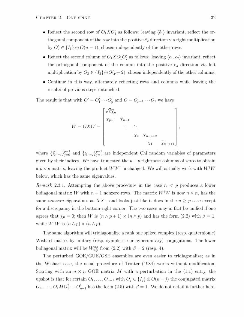
Chapter 2. One spike 32
• Reflect the second row of O1XO′1 as follows: leaving 〈e1〉 invariant, reflect the or-
thogonal component of the row into the positive e2 direction via right multiplication
by O′2 ∈ {I1} ⊕O(n− 1), chosen independently of the other rows.
• Reflect the second column of O1XO′1O′2 as follows: leaving 〈e1, e2〉 invariant, reflect
the orthogonal component of the column into the positive e3 direction via left
multiplication by O2 ∈ {I2}⊕O(p−2), chosen independently of the other columns.
• Continue in this way, alternately reflecting rows and columns while leaving the
results of previous steps untouched.
The result is that with O′ = O′1 · · ·O′p and O = Op−1 · · ·O1 we have
W = OXO′ =
√`χn
χp−1 χn−1. . . . . .
χ2 χn−p+2
χ1 χn−p+1
,
where {χn−j}p−1j=0 and {χp−j}p−1j=1 are independent Chi random variables of parameters
given by their indices. We have truncated the n−p rightmost columns of zeros to obtain
a p× p matrix, leaving the product WW † unchanged. We will actually work with W †W
below, which has the same eigenvalues.
Remark 2.3.1. Attempting the above procedure in the case n < p produces a lower
bidiagonal matrix W with n+ 1 nonzero rows. The matrix W †W is now n× n, has the
same nonzero eigenvalues as XX†, and looks just like it does in the n ≥ p case except
for a discrepancy in the bottom-right corner. The two cases may in fact be unified if one
agrees that χ0 = 0; then W is (n ∧ p + 1) × (n ∧ p) and has the form (2.2) with β = 1,
while W †W is (n ∧ p)× (n ∧ p).
The same algorithm will tridiagonalize a rank one spiked complex (resp. quaternionic)
Wishart matrix by unitary (resp. symplectic or hyperunitary) conjugations. The lower
bidiagonal matrix will be W β,`n,p from (2.2) with β = 2 (resp. 4).
The perturbed GOE/GUE/GSE ensembles are even easier to tridiagonalize; as in
the Wishart case, the usual procedure of Trotter (1984) works without modification.
Starting with an n × n GOE matrix M with a perturbation in the (1,1) entry, the
upshot is that for certain O1, . . . , On−1 with Oj ∈ {Ij}⊕O(n− j) the conjugated matrix
On−1 · · ·O1MO†1 · · ·O†n−1 has the form (2.5) with β = 1. We do not detail it further here.
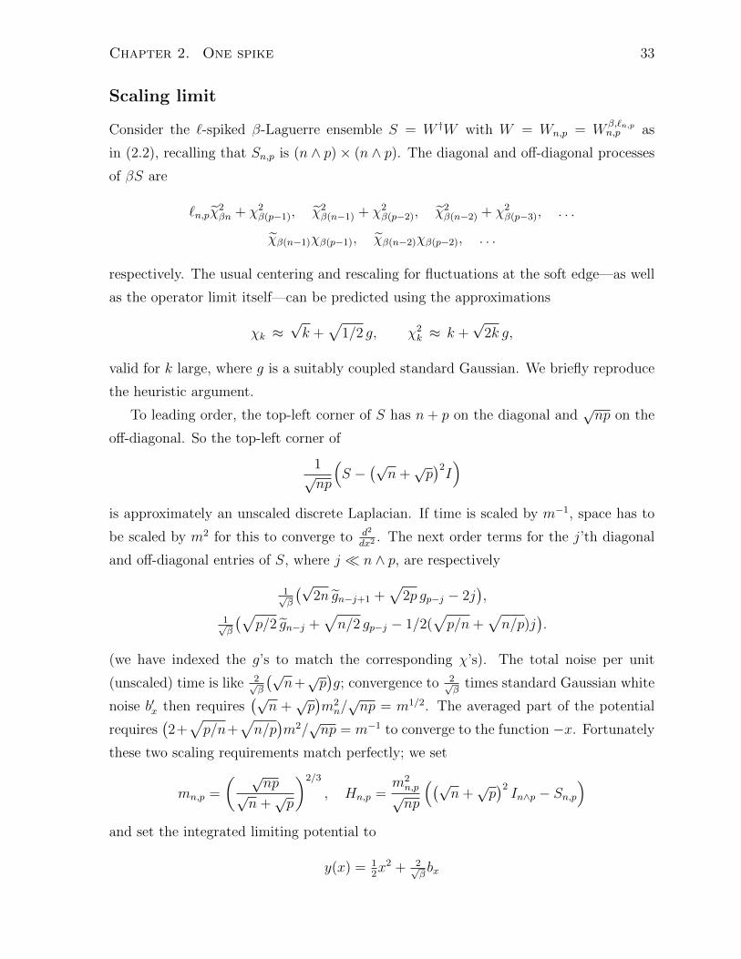
Chapter 2. One spike 33
Scaling limit
Consider the `-spiked β-Laguerre ensemble S = W †W with W = Wn,p = Wβ,`n,pn,p as
in (2.2), recalling that Sn,p is (n ∧ p)× (n ∧ p). The diagonal and off-diagonal processes
of βS are
`n,pχ2βn + χ2
β(p−1), χ2β(n−1) + χ2
β(p−2), χ2β(n−2) + χ2
β(p−3), . . .
χβ(n−1)χβ(p−1), χβ(n−2)χβ(p−2), . . .
respectively. The usual centering and rescaling for fluctuations at the soft edge—as well
as the operator limit itself—can be predicted using the approximations
χk ≈√k +
√1/2 g, χ2
k ≈ k +√
2k g,
valid for k large, where g is a suitably coupled standard Gaussian. We briefly reproduce
the heuristic argument.
To leading order, the top-left corner of S has n+ p on the diagonal and√np on the
off-diagonal. So the top-left corner of
1√np
(S −
(√n+√p)2I)
is approximately an unscaled discrete Laplacian. If time is scaled by m−1, space has to
be scaled by m2 for this to converge to d2
dx2. The next order terms for the j’th diagonal
and off-diagonal entries of S, where j � n ∧ p, are respectively
1√β
(√2n gn−j+1 +
√2p gp−j − 2j
),
1√β
(√p/2 gn−j +
√n/2 gp−j − 1/2(
√p/n+
√n/p)j
).
(we have indexed the g’s to match the corresponding χ’s). The total noise per unit
(unscaled) time is like 2√β
(√n+√p)g; convergence to 2√
βtimes standard Gaussian white
noise b′x then requires(√
n +√p)m2n/√np = m1/2. The averaged part of the potential
requires(2+√p/n+
√n/p)m2/√np = m−1 to converge to the function −x. Fortunately
these two scaling requirements match perfectly; we set
mn,p =
( √np
√n+√p
)2/3
, Hn,p =m2n,p√np
((√n+√p)2In∧p − Sn,p
)and set the integrated limiting potential to
y(x) = 12x2 + 2√
βbx
Chapter 2. One spike 34
where bx is a standard Brownian motion. Note that
2−2/3(n ∧ p)1/3 ≤ m ≤ (n ∧ p)1/3,
so the conditions m→∞, m = o(n ∧ p) are met by merely having n, p→∞ together.
We now carefully decompose Hn,p as in (2.11). In (2.12),(2.13) there is a little freedom
between yn,1;1 and wn, but only in to an additive constant in yn,1 that tends to zero in
probability anyway. Thus we may as well set yn,1;1 = 0 to fix wn and yn,i. Assumptions 1
and 2 (the CLT (2.14) and required tightness (2.15)–(2.17) for the potential terms yn,i)
are then verified as in the final subsection of RRV; Section 3.4 of the next chapter does
it in a more general setting with some clarifications and minor corrections.
It remains to consider Assumption 3. We have
wn = mn,p
(1 +
√n
p
(1− `n,p
χ2βn
βn
)+
√p
n
(1−
χ2β(p−1)
βp
)).
First order heuristics suggest we take `n,p to satisfy
wn = mn,p
(1 +
√n
p(1− `n,p)
)→ w ∈ (−∞,∞] as n ∧ p→∞
as in (2.4). We want to show that, in this case, wn → w in probability; it is certainly
enough to show that wn − wn → 0 in probability.
Second order heuristics say the error terms are on the order (n∧ p)−1/6 or m−1/2, and
L2 estimates easily provide the rigour. All we need is that χ2k has mean k and variance
2k. We have
wn − wn = − m`
β√np
(χ2βn − βn
)+
m
β√np
(β(p− 1)− χ2
β(p−1))
+m√np.
Using that ` ≤ 1 + 2√p/n, the mean square of the first term is O(m2/p+m2/n), which
is O(m−1). The mean square of the second term is O(m2/n), again O(m−1). The last
term is negligible. This completes the proof of Theorem 2.1.1.
Turning now to the perturbed β-Hermite ensemble, take Gn = Gβ,µnn as in (2.5). With
heuristic motivation similar to that in the previous proof, set
mn = n1/3, Hn =m2n√n
(2√nIn −Gn
)and y(x) as before. Decompose Hn as in (2.11). Again, the verification of Assumptions
1 and 2 on yn,i proceeds as in RRV (Lemmas 6.2, 6.3) or Section 3.4. Moving on to
Assumption 3, we have
wn = mn
(1−
(µn +
√2/βn g1
)).
Chapter 2. One spike 35
Putting
wn = mn (1− µn)
as in (2.6), the difference is wn − wn = −n−1/6√
2/β g1. It follows that wn − wn → 0 in
probability, which completes the proof of Theorem 2.1.5.
2.4 Alternative characterizations of the laws
In this section we prove Theorem 2.1.7 and its extension to higher eigenvalues.
Diffusion
The diffusion characterization is developed in RRV; we recall the important facts here
with a general initial condition. For a fully rigorous treatment see Appendix A. The
starting point is an application of the classical Riccati map p = f ′/f to the eigenvalue
equation (2.20), or rigorously to (2.24); the result is the first order differential equation
p′(x) = x− λ+ 2√βb′(x)− p2(x) (2.28)
understood also in the integrated sense. The boundary condition at the origin becomes
the initial value
p(0) = w,
and a zero of f would have p explode to −∞ and immediately restart at +∞.
One can in fact construct the solution for any λ ∈ R. One way to see this is to
introduce the variable q(x) = p(x) + 2√βb(x); the ODE
q′ = x− λ−(q + 2√
βb)2
(2.29)
is classical and the Picard existence and uniqueness theorem applies. Although solutions
can explode to −∞ in finite time, this is not a problem if we consider the values on the
projective line. Behaviour through ∞ can then be understood in the other coordinate
q = 1/q, which evolves as
q′ =(1 + 2√
βbq)2 − (x− λ)q2;
in particular, q′ = 1 whenever q = 0. The solution can thus be continued for all time.
Moreover, it depends monotonically and continuously on the the parameter λ, uniformly
Chapter 2. One spike 36
on compact time-intervals with respect to the topology of the projective line. Following
classical Sturm oscillation theory one can argue that almost surely, for all λ ∈ R, the
number of eigenvalues strictly less than λ equals the number of explosions of p on R+.
For a fixed λ, the Riccati equation (2.28) may also be understood in the Ito sense;
by translation equivariance the time-shift x 7→ x−λ produces the same path measure as
the Ito diffusion (2.7) started at time x0 = −λ. Writing κ(x0,w0) for the distribution of
the first explosion time of px under P(x0,w0)—an improper distribution with some mass
on ∞—we have Pβ,w(Λ0 < λ) = κ(−λ,w)(R) or Fβ,w(x) = κ(x,w)({∞}) as in (2.8). More
generally, the strong Markov property gives
Pβ,w(−Λk−1 > x) =
∫Rkκ(x,w)(dx1)κ(x1,∞)(dx2) · · · κ(xk−1,∞)(dxk). (2.30)
The stated path properties of (2.7) appear also in RRV (Propositions 3.7 and 3.9).
Boundary value problem
Briefly, the boundary value problem is just the Kolmogorov backward equation for a
hitting probability of the diffusion. We assume the diffusion representation Fβ,w(x) =
κ(x,w)({∞}) for the distribution of −Λ0.
Lemma 2.4.1. For each fixed x, Fβ,w(x) is nondecreasing and continuous in w ∈ (∞,∞]
and tends to zero as w → −∞.
Remark 2.4.2. There are in fact almost-sure counterparts of these assertions that describe
how Λ0 depends on w for each Brownian path, but we do not need them here.
Proof. The monotonicity is a consequence of uniqueness of the diffusion path from each
space-time point: two paths started from (x,w0) and (x,w1) with w0 < w1 never cross, so
if the upper path explodes to −∞ then the lower path must do so as well. The continuity
is a general property of statistics of diffusions: κ(x,px)({∞}) is a martingale, so Fβ,w(x)
is in fact space-time harmonic. (Again, the behaviour at w = +∞ may be understood
by changing coordinates.)
The final assertion is that for fixed x0 explosion becomes certain as w → −∞. It
may be verified by a domination argument involving the ODE (2.29) (time-shifted as
above so that λ = 0 and the initial time is x0), whose paths explode simultaneously with
those of (2.7). Given ε > 0, let M be such that P(supx∈[x0,x0+1] |bx| > M) < ε. It is
easy to check that for r0 sufficiently negative, the solution of r′ = x − (r + M)2 with
Chapter 2. One spike 37
initial value r(x0) = r0 explodes to −∞ before time x0 + 1. Now consider the solution of
q′ = x − (q + b)2 with q(x0) ≤ r0 ≤ −M . With probability 1 − ε we have q′(x) ≤ r′(x)
whenever q(x) = r(x), so the paths never cross and q explodes as well.
Proof of Theorem 2.1.7 (ii). Writing L for the space-time generator of the SDE (2.7), the
PDE (2.9) is simply the equation LF = 0. Therefore the hitting probability F (x,w) =
Fβ,w(x) satisfies the PDE. The boundary behaviour (2.10) follows from Lemma 2.4.1
and the fact that F (·, w) is a distribution function for each w. Specifically, the lower
part of the boundary behaviour follows from the fact that F (x,w) is increasing in x and
F (x,w)→ 0 as w → −∞ for each x. The upper part follows from the fact that F (x,w)
is increasing in w and F (x,w)→ 1 for fixed w as x→∞.
Toward uniqueness, suppose F (x,w) is another bounded solution of (2.9),(2.10). By
the PDE, F (x, px) is a local martingale under P(x0,w0) and thus a bounded martingale. Let
T be the lifetime of the diffusion; optional stopping gives F (x,w) = E(x,w) F (T ∧ t, pT∧t)for all t ≥ x. Taking t → ∞, we conclude by bounded convergence, the boundary
behaviour of F and the stated path properties of the diffusion that F (x,w) is the non-
explosion probability. That is, F = F .
As promised, we indicate how the laws of the higher eigenvalues Λ1,Λ2, . . . may be
characterized in terms of the PDE (2.9). The characterization is inductive and follows
from (2.30) by reasoning just as in the preceding proof.
Theorem 2.4.3. Let F(0)(x,w) = Pβ,w(−Λ0 < x). For each k = 1, 2, . . ., the boundary
value problem
∂F
∂x+
2
β
∂2F
∂w2+(x− w2
)∂F∂w
= 0 for (x,w) ∈ R2,
F (x,w)→
1 as x,w →∞ together,
F(k−1)(x0,+∞) as w → −∞ while x→ x0 ∈ R
has a unique bounded solution F(k), and we have Pβ,w(−Λk < x) = F(k)(x,w) for w ∈(−∞,∞); further, Pβ,∞(−Λk < x) = limw→∞ F(k)(x,w).
Chapter 3
Several spikes
3.1 Introduction
We refer the reader to the introduction of Chapter 2 for background on the spiked Wishart
model introduced by Johnstone (2001) in the context of high-dimensional data analysis,
especially the phase transition phenomenon that Baik, Ben Arous and Peche (2005)
(BBP) described in the complex case. We refer the reader to the same place for back-
ground on the stochastic Airy operator introduced by Sutton (2005), Edelman and Sutton
(2007), and its development byRamırez, Rider and Virag (2011) (RRV) that we build
on.
In Chapter 2 we considered rank one spiked real/complex/quaternion Wishart matri-
ces and additive rank one perturbations of the Gaussian orthogonal, unitary and sym-
plectic ensembles. We introduced their general β analogues in terms of “spiked” versions
of the tridiagonal ensembles of Dumitriu and Edelman (2002) and extended the RRV
technology to describe the soft-edge scaling limit in terms of the stochastic Airy operator
− d2
dx2+ 2√
βb′x + x
on L2(R+) with a boundary condition depending on the spike. The boundary condition
changes from Dirichlet f(0) = 0 to Neumann/Robin f ′(0) = wf(0) at the onset of the
BBP phase transition, with w ∈ R representing a scaling parameter for perturbations in
a “critical window”. The resulting largest eigenvalue laws form a one-parameter family
of deformations of Tracy-Widom(β), naturally generalizing the characterization of RRV
in terms of the ground state of this random Schrodinger operator. We went on to char-
acterize the limit laws in terms of the diffusion from RRV and further in terms of an
38
Chapter 3. Several spikes 39
associated second-order linear parabolic PDE.
Here we deal with r “spikes”, or general bounded-rank perturbations of Gaussian and
Wishart matrices. To do so we introduce a new “canonical form for perturbations in a
fixed subspace”, a (2r+1)-diagonal band form that has a purely algebraic interpretation.
It generalizes the Dimitriu–Edelman forms and is able to handle rank r perturbations.
We then develop a generalization of the methods of RRV and Chapter 2 to a matrix-
valued setting: block tridiagonal matrices converge to a half-line Schrodinger operator
with matrix-valued potential, the spikes once again appearing in the boundary condition.
We treat the real, complex and quaternion (β = 1, 2, 4) cases simultaneously. Once again,
even the existence of a near-critical soft-edge limit is new off β = 2. Unlike in Chapter 2,
however, we do not define a general β version of either matrix model, nor of the limiting
operator; we will see that in the higher rank cases these objects do not readily admit a
β-generalization.
Dyson’s Brownian motion makes a surprise appearance, providing nice SDE and PDE
characterizations of the limit laws—r parameter deformations of Tracy-Widom(β)—in
which β reappears as a simple parameter. The derivation makes use of the matrix versions
of classical Sturm oscillation theory and the Riccati transformation.
We highlight two more features of our approach beyond the novelty of bypassing
joint densities and handling β = 1, 2, 4 together. First, we treat the perturbation as a
parameter. By this we mean that all perturbations in a fixed subspace are considered
jointly (on the same probability space); this picture is carried through to the limit, which
is therefore a family of point processes parametrized by an r×r matrix. Second, we allow
more general scalings than those considered in BBP. Most importantly, in the Wishart
case we do not require the two dimensional parameters n, p to have a positive limiting
ratio but rather allow them to tend to infinity together arbitrarily.
To state our results we introduce some objects and notation that will be used through-
out the chapter.
Let F = R, C, or H and β = 1, 2 or 4, respectively. A standard F Gaussian Z ∼FN(0, 1) is an F-valued random variable described in terms of independent real Gaussians
g1, . . . , gβ ∼ N(0, 1) as g1 for F = R, (g1 +g2i)/√
2 for F = C, and (g1 +g2i+g3j+g4k)/2
for F = H. Note that in each case E |Z|2 = 1 and uZ ∼ FN(0, 1) for u ∈ F with
|u|2 = u∗u = 1.
The space of column vectors Fn is endowed with the standard inner product u†v and
associated norm |u|2 = u†u (we reserve double bars for function spaces). Write FNn(0, I)
Chapter 3. Several spikes 40
for a vector of independent standard F Gaussians. With Σ ∈Mn(F) positive definite, we
write Z ∼ FNn(0,Σ) for Z = Σ1/2Z0 with Z0 ∼ FNn(0, I).
Define the unitary group Un(F) = {U ∈ Fn×n : U †U = I}, better known as the
orthogonal, unitary or symplectic group for F = R, C, H respectively. It acts on Fn by
left multiplication, on which the distribution FNn(0, I) is invariant. Write Mn(F) = {A ∈Fn×n : A† = A} for the self-adjoint matrices, also known as real symmetric, complex
hermitian or quaternion self-dual. Un(F) acts on Mn(F) by conjugation.
The Gaussian orthogonal/unitary/symplectic ensemble (GO/U/SE) is the
probability measure on Mn(F) described by A = (X + X†)/√
2 where X is an n × n
matrix of independent FN(0, 1) entries. The distribution is invariant under the unitary
action. Furthermore, the algebraically independent entries Aij, i ≥ j are statistically
independent. (Together, this invariance and independence characterizes the distribution
up to a scale factorr.) For an entry-wise description, the diagonal entries are distributed
as N(0, 2/β) while the off-diagonal entries are FN(0, 1).
Fixing a positive integer r, we study rank r additive perturbations A = A0 + P
of a GO/U/SE matrix A0, where P = P ⊕ 0n−r with P ∈ Mr(F) nonrandom. We will
be interested in the eigenvalues λ1 ≥ · · · ≥ λn of A. Of course for a single P their
distribution depends only on the eigenvalues of P , but we consider them jointly over all
P .
We also consider real/complex/quaternion Wishart matrices. These are ran-
dom nonnegative matrices in Mp(F) given by XX† where the data matrix X is p × nwith n independent FNp(0,Σ) columns. We speak of a p-variate Wishart with n de-
grees of freedom and p× p covariance Σ > 0. Since we are interested in the nonzero
eigenvalues λ1 ≥ · · · ≥ λn∧p, we can equally well consider X†X. The distribution of X†X
may also be described as X†0ΣX0 where X0 is a p × n matrix of independent FN(0, 1)
entries. The case Σ = I is referred to as the null case. We study the rank r spiked
case where Σ = Σ⊕ Ip−r with Σ ∈Mr(F) nonrandom. Once again the eigenvalue distri-
bution depends only on the eigenvalues of Σ, but we consider the spectrum jointly as Σ
varies.
Our starting point is a new banded or multidiagonal form introduced in Section 3.2,
ideally suited to the types of perturbations we consider. It is defined for almost every
matrix A ∈ Mn(F); given vectors v1, . . . , vr ∈ Fn, the new basis may be obtained by
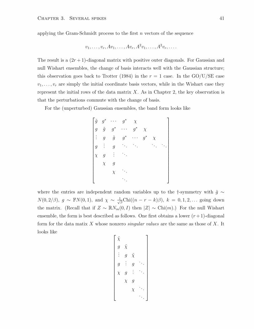
Chapter 3. Several spikes 41
applying the Gram-Schmidt process to the first n vectors of the sequence
v1, . . . , vr, Av1, . . . , Avr, A2v1, . . . , A
2vr, . . . .
The result is a (2r+ 1)-diagonal matrix with positive outer diagonals. For Gaussian and
null Wishart ensembles, the change of basis interacts well with the Gaussian structure;
this observation goes back to Trotter (1984) in the r = 1 case. In the GO/U/SE case
v1, . . . , vr are simply the initial coordinate basis vectors, while in the Wishart case they
represent the initial rows of the data matrix X. As in Chapter 2, the key observation is
that the perturbations commute with the change of basis.
For the (unperturbed) Gaussian ensembles, the band form looks like
g g∗ · · · g∗ χ
g g g∗ · · · g∗ χ... g g g∗ · · · g∗ χ
g... g
. . . . . . . . . . . .
χ g...
. . .
χ g
χ. . .. . .
where the entries are independent random variables up to the †-symmetry with g ∼N(0, 2/β), g ∼ FN(0, 1), and χ ∼ 1√
βChi((n − r − k)β), k = 0, 1, 2, . . . going down
the matrix. (Recall that if Z ∼ RNm(0, I) then |Z| ∼ Chi(m).) For the null Wishart
ensemble, the form is best described as follows. One first obtains a lower (r+1)-diagonal
form for the data matix X whose nonzero singular values are the same as those of X. It
looks like
χ
g χ... g χ
g... g
. . .
χ g...
. . .
χ g
χ. . .. . .
Chapter 3. Several spikes 42
where the entries are independent random variables with g ∼ FN(0, 1), χ ∼ 1√βChi((n−
k)β) and χ ∼ 1√βChi((n − r − k)β), k = 0, 1, 2, . . . going down the matrix. One then
forms its multiplicative symmetrization, a (2r+1)-diagonal matrix with the same nonzero
eigenvalues as X. In both cases the perturbations appear in the upper-left r × r block.
Section 3.2 provides derivations. The obstacle to β-generalization at this level is the
presence of F Gaussians in the intermediate diagonals.
Proceeding with an analogue of the RRV convergence result hinges on reinterpreting
these forms as block tridiagonal with r × r blocks. In Section 3.3 we develop an Mr(F)-
valued analogue of the RRV technology, providing general conditions under which the
principal eigenvalues and corresponding eigenvectors of such a random block tridiagonal
matrix converge to a those of a continuum half-line random Schrodinger operator with
matrix-valued potential. As in Chapter 2 we allow for a general boundary condition at
the origin.
In Section 3.4 we apply this result to the band forms just described, proving a process
central limit theorem for the potential and verifying the required tightness assumptions.
The limiting operator turns out to be a multidimensional version of the stochastic Airy
operator, which we now describe.
First, a standard F Brownian motion {bt}t≥0 is a continuous F-valued random
process with b0 = 0 and independent increments bt − bs ∼ FN(0, t − s). (It can be
described in terms of β = 1, 2 or 4 independent standard real Brownian motions.) A
standard matrix Brownian motion {Bt}t≥0 has continuous Mn(F)-valued paths with
B0 = 0 and independent increments Bt − Bs distributed as√t− s times a GO/U/SE.
The diagonal processes are thus√
2/β times standard real Brownian motions while the
off-diagonal processes are standard F Brownian motions, mutually independent up to
symmetry.
Finally, we define the multivariate stochastic Airy operator. Operating on the
vector-valued function space L2(R+,Fr) with inner product 〈f, g〉 =∫∞0f †g and associ-
ated norm ‖f‖2 =∫∞0|f |2, it is the random Schrodinger operator
Hβ = − d2
dx2+√
2B′x + rx (3.1)
where B′x is “standard matrix white noise”, the derivative of a standard matrix Brownian
motion, and rx is scalar. (Here again β is restricted to the classical values, as the noise
term lacks a straightforward β-generalization.) The potential is thus the derivative of
a continuous matrix-valued function; rigorous definitions will appear in Section 3.3 in a
Chapter 3. Several spikes 43
more general setting.
For now it is enough to know that, together with a general self-adjoint boundary
condition
f ′(0) = Wf(0), (3.2)
the multivariate stochastic Airy operator is bounded below with purely discrete spec-
turm given by a variational principle. Here W ∈ Mr(F); actually, writing the spectral
decomposition W =∑r
i=1wiuiu†i , we formally allow wi ∈ (−∞,∞]. Writing fi = u†if ,
(3.2) is then to be interpreted as
f ′i(0) = wifi(0) for wi ∈ R
fi(0) = 0 for wi = +∞.
We write W ∈M∗r (F) for this extended set and Hβ,W for (3.1) together with (3.2).
For concreteness, we record that the eigenvalues Λ0 ≤ Λ1 ≤ . . . and correspond-
ing eigenfunctions f0, f1, . . . of Hβ,W are given respectively by the minimum and any
minimizer in the recursive variational problem
inff∈L2(R+)
‖f‖=1, f⊥f0,...,fk−1
∫ ∞0
(|f ′|2 + rx |f |2
)dx+ f(0)†Wf(0) + 2√
β
∫ ∞0
f †dBxf.
Here canidates f are only considered if the first integral and boundary term are finite; the
stochastic integral can then be defined pathwise via integration by parts. The eigenvalues
and eigenfunctions are thus jointly defined random processes indexed over W .
Remark 3.1.1. We note one important property of the eigenvalue processes, namely the
pathwise monotonicity of Λk in W with respect to the usual matrix partial order. This is
immediate from the variational characterization and the fact that the objective functional
is monotone in W . (For the higher eigenvalues it is most apparent from the standard
min-max formulation of the variational problem.)
We can now state the main convergence results. As outlined, Sections 3.2–3.4 furnish
the proofs. One last shorthand: when we write that a sequence Wn ∈ Mr(F) tends to
W ∈M∗r (F), we mean the following. Writing W =
∑ri=1wiuiu
†i with wi ∈ (−∞,∞], one
has Wn =∑r
i=1wn,iuiu†i with wn,i ∈ R satisfying wn,i → wi for each i. In other words,
the matrices are simultaneously diagonal and the eigenvalues tend to the corresponding
limits.
Chapter 3. Several spikes 44
Theorem 3.1.2. Let A = A0 +√nPn where A0 is an n × n GO/U/SE matrix and
Pn = Pn ⊕ 0n−r with Pn ∈Mr(F), and let λ1 ≥ · · · ≥ λn be its eigenvalues. If
n1/3(1− Pn) → W ∈M∗
r (F) as n→∞
then, jointly for k = 1, 2, . . . in the sense of finite-dimensional distributions,
n1/6(λk − 2
√n)⇒ −Λk−1 as n→∞
where Λ0 ≤ Λ1 ≤ . . . are the eigenvalues of Hβ,W . Convergence holds jointly over
{Pn},W satisfying the condition.
Theorem 3.1.3. Consider a p-variate real/complex/quaternion Wishart matrix with n
degrees of freedom and spiked covariance Σn,p = Σn,p ⊕ Ip−r > 0 with Σn,p ∈ Mr(F), and
let λ1 ≥ · · · ≥ λn∧p be its nonzero eigenvalues. Writing mn,p = (n−1/2 + p−1/2)−2/3, if
mn,p
(1−
√n/p(Σn,p − 1
))→ W ∈M∗
r (F) as n→∞
then, jointly for k = 1, 2, . . . in the sense of finite-dimensional distributions,
m2n,p√np
(λk − (
√n+√p)2)⇒ −Λk−1 as n→∞
where Λ0 ≤ Λ1 ≤ . . . are the eigenvalues of Hβ,W . Convergence holds jointly over
{Σn,p},W satisfying the condition.
Remark 3.1.4. In the band basis described above, we also have joint convergence of the
corresponding eigenvectors to the eigenfunctions of Hβ,W . In detail, the eigenvectors
should be embedded in L2(R+) as step functions with step width n−1/3 in the Gaussian
case and m−1n,p in the Wishart case, and convergence is in law with respect to the L2 norm
topology. To be precise, one should use either subsequences or spectral projections; one
could also formulate the joint eigenvalue-eigenvector convergence in terms of the norm
resolvent topology. See Theorem 3.3.9 and the remark that follows.
We now give the two promised alternative characterizations of the limiting eigenvalue
laws. Fix β = 1, 2, 4 and W ∈ M∗r (F) with eigenvalues −∞ < w1 ≤ . . . ≤ wr ≤ ∞.
Writing P for the probability measure associated with Hβ,W and its spectrum {Λ0 ≤Λ1 ≤ . . .}, let
F kβ (x;w1, . . . , wr) = P(−Λk ≤ x)
for k = 0, 1, . . .. Write simply Fβ = F 0β for the ground state distribution (limiting largest
eigenvalue law). Once again, the generalization from Chapter 2 is not straightforward.
The proofs are contained in Section 3.5.
Chapter 3. Several spikes 45
Theorem 3.1.5. Let Px0,(w1,...,wr) be the measure on paths (p1, . . . , pr) : [x0,∞) →(−∞,∞]r determined by the coupled diffusions
dpi = 2√βdbi +
(rx− p2i +
∑j 6=i
2
pi − pj
)dx (3.3)
with initial conditions pi(x0) = wi and entering into {p1 < . . . < pr}, where b1, . . . , br are
independent standard Brownian motions; particles pi may explode to −∞ in finite time
whereupon they are restarted at +∞. Then
Fβ(x;w1, . . . , wr) = Px/r,(w1,...,wr)(no explosions). (3.4)
More generally,
F kβ (x;w1, . . . , wr) = Px/r,(w1,...,wr)(at most k explosions). (3.5)
We describe the diffusion more carefully in Section 3.5, asserting that it determines
a law on paths valued in an appropriate space. Probabilistic arguments lead to the
following reformulation in terms of its generator.
Theorem 3.1.6. Fβ(x;w1, . . . , wr) is the unique bounded function F : R × Rr → Rsymmetric with respect to permutation of w1, . . . , wr that satisfies the PDE
r∂F
∂x+
r∑i=1
(2
β
∂2F
∂w2i
+ (x− w2i )∂F
∂wi
)+∑i<j
2
wi − wj
(∂F
∂wi− ∂F
∂wj
)= 0 (3.6)
and the boundary conditions
F → 1 as x→∞ with w1, . . . , wr bounded below; (3.7)
F → 0 as any wi → −∞ with x bounded above. (3.8)
Furthermore, Fβ is “continuous to the boundary” as one or several wi → +∞. For
subsequent eigenvalue laws F kβ (x;w1, . . . , wr), (3.8) is replaced with the recursive boundary
condition
F k(x;w1, . . . , wr)→ F k−1(x∗;w∗1, . . . , w∗r−1,+∞)
as x→ x∗ ∈ R, wi → w∗i ∈ R for i = 1, . . . , r − 1, and wr → −∞.(3.9)
At β = 2 these distributions were obtained in BBP in the form of Fredholm deter-
minants of finite-rank perturbations of the Airy kernel. Baik (2006) derived Painleve II
Chapter 3. Several spikes 46
formulas, and by a symbolic computation with the computer algebra system Maple we
were able to verify that the latter satisfy the PDE (3.6) for r = 2, 3, 4, 5. We give the
details in Section 5.3 of Chapter 5. Of course a pencil-and-paper proof for all r would be
more illuminating and certainly more satisfying.
We make two final remarks. From the finite n matrix models it is clear that the
“rank r deformed” limiting distributions Fβ,r(x;w1, . . . , wr) reduce to those for a lower
rank r0 < r in the following way:
Fβ,r(x;w1, . . . , wr0 ,+∞, . . . ,+∞) = Fβ,r0(x;w1, . . . , wr0).
Unfortunately this reduction relation is not readily apparent from any of our characteri-
zations (operator, SDE or PDE).
Lastly, the SDE and PDE characterizations seem to make sense for all β > 0 (although
one has to be careful for β < 1). It would be interesting to find natural “general β
multispiked models” at finite n, interpolating between those studied here at β = 1, 2, 4
and generalizing those introduced in Chapter 2 for r = 1. At β = 2, perhaps one could
discover a relationship with formulas of Baik and Wang (2011).
3.2 A canonical form for perturbation in a fixed sub-
space
In Chapter 2 we observed that the tridiagonal models of Gaussian and Wishart matrices
were amenable to rank one perturbation. In this section we introduce a banded (also block
tridiagonal) generalization amenable to higher-rank perturbation. We first describe it as
a natural object of pure linear algebra; we then show how it interacts with the structure
of Gaussian and Wishart random matrices to produce the band forms displayed in the
introduction.
The basic facts of “linear algebra over F”, where F may be R, C or the skew field of
quaternions H, are summarized in Appendix E of Anderson et al. (2009). Everything we
need (inner product geometry, self-adjointness, eigenvalues, and the spectral theorem)
simply works over H as expected, keeping in mind only that non-real scalars may not
commute.
Chapter 3. Several spikes 47
The band Jacobi form as an algebraic object
We present a natural “canonical form” for studying perturbations in a fixed subspace of
dimension r. It is a (2r+1)-diagonal band matrix generalizing the symmetric tridiagonal
Jacobi form, which is the r = 1 case. The outermost diagonals continue to be positive;
however, intermediate diagonals between the main and outermost ones are not in general
real. Once again, the presence of F Gaussians is the obstacle to writing down a general
β analogue.
We begin with a geometric, coordinate-free formulation.
Theorem 3.2.1. Let T be a self-adjoint linear transformation on a finite-dimensional
inner product space V of dimension n over F. An orthonormal sequence {v1, . . . , vr} ⊂ V
with 1 ≤ r ≤ n can be extended to an ordered orthonormal basis {v1, . . . , vn} for V such
that 〈vi, T vj〉 ≥ 0 for |i− j| = r and 〈vi, T vj〉 = 0 for |i− j| > r. Furthermore, if
〈vi, T vj〉 > 0 for |i− j| = r then the extension is unique.
The point is that the same extension works for T ′ = T + P provided P ∈ Mn(F)
satisfies P∣∣{v1,...,vr}⊥
= 0. In this case span{v1, . . . , vr} is also an invariant subspace of P
and we speak of perturbing in this subspace.
Proof. We give an explicit inductive construction. Along the way we will see that the
uniqueness condition holds precisely when the choice is forced at each step.
It is convenient to restate the properties of the orthonormal basis in the theorem in
the following equivalent way: For r + 1 ≤ i ≤ n we have 〈vi, T vi−r〉 ≥ 0 and Tvi−r ∈span{v1, . . . , vi}. Suppose inductively that v1, . . . , vk−1 have been obtained for some
r+ 1 ≤ k ≤ n, satisfying the preceding conditions for r+ 1 ≤ i ≤ k− 1. Let w = Tvk−r;
we must choose vk so that 〈vk, w〉 ≥ 0 and w ∈ span{v1, . . . , vk}. There are two cases to
consider. If w /∈ span{v1, . . . , vk−1} then vk must be a multiple of w′ = w−∑k−1
i=1 〈vi, w〉 vi;the positivity condition further forces vk = w′/ |w′|, which gives 〈vk, w〉 = |w′| > 0. If
w ∈ span{v1, . . . , vk−1} then any vk ∈ {v1, . . . , vk−1}⊥ will do, and in this case 〈vk, w〉 =
0.
Remark 3.2.2. When uniqueness holds, as is generically the case, the basis may also be
obtained by applying the Gram-Schmidt process to the first n vectors of the sequence
v1, . . . , vr, T v1, . . . , T vr, T2v1, . . . , T
2vr, . . . .
Chapter 3. Several spikes 48
We now state and prove a concrete matrix formulation in which the first r coordinate
vectors play the role of v1, . . . vr. The point of the second proof is that it emphasizes the
resulting band matrix rather than the change of basis; the algorithm will be used in the
next subsection.
Theorem 3.2.3. Let A ∈ Mn(F) and 1 ≤ r ≤ n. There there exists U ∈ Un(F) of the
form U = Ir ⊕ U with U ∈ Un−r(F) such that B = UAU † satisfies
Bij ≥ 0 for 1 ≤ i, j ≤ n with |i− j| = r, (3.10)
Bij = 0 for 1 ≤ i, j ≤ n with |i− j| > r. (3.11)
Furthermore, if strict positivity holds in (3.10) then U and B as such are unique.
We refer to B as the band Jacobi form of A. The allowed perturbations here have
the form P = P ⊕ 0n−r for P ∈ Mr(F); these are invariant under conjugation by U , so
U(A+ P )U † = B + P .
Proof. We prove existence by giving an explicit algorithm; it generalizes the Lanczos
algorithm, which applies in the case r = 1.
• For the first step, let v = [Ai,1]r+1≤i≤n ∈ Fn−r and take U ∈ Un−r(F) such that
Uv = |v|e1, where e1 is the first standard basis vector of Fn−r. A concrete choice
is the Householder reflection U = In−r − 2ww†/w†w with w = v − |v|e1. Set
U1 = Ir ⊕ U and B1 = U1AU†1 .
• Continue inductively: Having obtained Uk, Bk, let v = [(B1)i,(k+1)]r+k+1≤i≤n ∈Fn−r−k and take U ∈ Un−r−k(F) such that Uv = |v|e1. Set Uk+1 = Ir+k ⊕ U and
Bk+1 = Uk+1BkU†k+1.
• Stop when k = n− r. Let U = Un−r · · ·U1 and B = Bn−r = UAU †.
It is immediate that U and B have the required properties. The point is that the kth
column of Bk already “looks right”, i.e. (Bk)r+k,k ≥ 0 and (Bk)r+l,k = 0 for l > k, and
subsequent transformations Uk+1, . . . , Un−k ∈ {Ir+k} ⊕ Un−r−k(F) “don’t mess it up.”
Towards uniqueness, suppose that U ′, B′ = U ′AU ′† also have the required properties
and let W = U ′U−1 so that B′ = WBW †. Assume inductively that W ∈ {Ir+k} ⊕Un−r−k(F), which is certainly true in the base case k = 0. Write W = Ir+k ⊕ W . Let
b = [Bi,k+1]r+k+1≤i≤n ∈ Fn−r−k and similarly for b′. Then b′ = W b. But b = ae1 and
Chapter 3. Several spikes 49
b′ = a′e1 with a, a′ > 0 by assumption. It follows that a = a′ and W e1 = e1. Hence
W ∈ {I1} ⊕ Un−r−(k+1)(F) and W ∈ {Ir+k+1} ⊕ Un−r−(k+1)(F), completing the induction
step. We conclude that W = In.
Perturbed Gaussian and spiked Wishart models
The change of basis described above interacts very nicely with the Gaussian structure
in Gaussian and Wishart random matrices. The r = 1 case of this observation is due
to Trotter (1984), who described the tridiagonal forms explicitly. His forms fall into the
framework of Theorem 3.2.1 by taking the initial vector to be fixed in the Gaussian case,
and taking it to be the top row of the data matrix in the Wishart case. As we observed
in Chapter 2, the change of basis commutes with rank one additive perturbations for the
Gaussian case and with rank one spiking for the Wishart case. We now extend the story
to the r > 1 setting.
In the Gaussian case we will be perturbing in a fixed (non-random) subspace; without
loss of generality this may be taken as the initial r-dimensional coordinate subspace, and
so we take the basis of Theorem 3.2.1 that begins with the first r standard basis vectors.
We can therefore obtain the band form by a direct application of the algorithm from the
proof of Theorem 3.2.3. The Wishart case is a little more complicated; here we want to
perturb in the random subspace spanned by the first r rows of the data matrix. Our new
basis will begin with the Gram-Schmidt orthogonalization of these initial rows. As in
the r = 1 case it is most transparent to construct a lower band form of the data matrix
first, afterwards realizing the band Jacobi form as its multiplicative symmetrization. In
both the Gaussian and the Wishart cases we will see that the uniqueness condition of
Theorem 3.2.1 holds almost surely.
Let A be an n × n GOE matrix. Applying the algorithm from the proof of Theo-
rem 3.2.3 while keeping track of the distribution of the matrix Bk at each step—the key
of course being the unitary invariance of standard Gaussian vectors—yields the following
Chapter 3. Several spikes 50
band Jacobi random matrix G = UAU †:
Gij =
√2βgi i = j
gij j < i < j + r
1√βχ(n−i+1)β i = j + r
0 i > j + r
G∗ji i < j
(3.12)
for 1 ≤ i, j ≤ n, where the random variables appearing explicitly are independent,
gi ∼ N(0, 1), gij ∼ FN(0, 1), and χk ∼ Chi(k). The latter is the distribution of the
length of a k-dimensional standard Gaussian vector.
We can introduce a rank r additive perturbation A = A0 +√nP , where P = P ⊕0n−r
with P ∈Mr(F); since P commutes with the change of basis U ∈ {Ir}⊕Un−r(F), we can
write
G = UAU † = U(A0 +√nP )U † = UA0U
† +√nP = G0 +
√nP. (3.13)
As expected the perturbation shows up undisturbed in the upper-left r × r corner of G
Turning to the Wishart case, we first consider the null Wishart random matrix X†X,
where X is p×n with independent FN(0, 1) entries. (Remember that X†X and XX† have
the same nonzero eigenvalues λ1, . . . , λn∧p.) The final form can be described abstractly
as given in the basis of Theorem 3.2.1 that extends the Gram-Schmidt orthogonaliza-
tion of the first r rows of X. One cannot readily obtain a description of the resulting
random matrix from here, however, so we give another way that generalizes Trotter’s
original procedure. It is a “singular value analogue” of the algorithm from the proof of
Theorem 3.2.3, producing matrices U ∈ Un(F) and V ∈ Up(F) such that L = V XU has
a “lower band form” that is zero off the main and first r subdiagonals and positive on
the outermost of these. The key is to work alternately on rows and columns.
• Take U1 ∈ Un(F) so that the first row of XU1 lies in the (positive) direction of the
first coordinate basis vector of Fn.
• Take V1 = Ir ⊕ Up−r(F) so that [(V1XU1)i,1]r+1≤i≤p ∈ Fp−r lies in the direction of
the first coordinate basis vector of the latter subspace.
• Take U2 ∈ I1 ⊕ Un−1(F) so that [(V1XU1U2)2,j]2≤j≤n ∈ Fn−1 lies in the direction of
the first coordinate basis vector of the latter subspace.
Chapter 3. Several spikes 51
• Take V2 ∈ Ir+1 ⊕ Up−r−1(F) so that [(V2V1XU1U2)i,2]r+2≤j≤p ∈ Fp−r−1 lies in the
direction of the first coordinate basis vector of the latter subspace.
• Continue in this way until the rows and columns both run out (stop alternating if
one runs out before the other).
The resulting L = Vn∧(p−r) · · ·V1XU1 · · ·Un∧p has n ∧ p nonzero columns and (n+ r) ∧ pnonzero rows, which can be described as follows:
Lij =
1√βχ(n−i+1)β i = j
gij j < i < j + r
1√βχ(p−i+1)β i = j + r
0 i < j or i > j + r
(3.14)
where the entries are independent, χk, χk ∼ Chi(k), gij ∼ FN(0, 1). Truncating the
remaining zero rows or columns, the matrix S = L†L is (n ∧ p) × (n ∧ p) and has the
same nonzero eigenvalues as X†X. It has the band form
Sij =
1βχ2(n−i+1)β +
∑i<k<i+r |gk,i|
2 + 1βχ2(p−i−r+1)β i = j
1√βχ(n−i+1)βgij +
∑i<k<j+r g
∗k,igk,j + 1√
βg∗j+r,iχ(p−j−r+1)β j < i < j + r
1βχ(n−i+1)βχ(p−i+1)β i = j + r
0 i > j + r
S∗ji i < j
(3.15)
where we have ignored the issue of truncation in the final r rows and columns (g′s and χ′s
with indices beyond the allowed range should simply be zero). The change of basis is thus
U1 · · ·Un∧p; a little thought shows that, as claimed earlier, the new basis begins with the
orthogonalization of the first r rows of X. Since the form (3.15) satisfies the uniqueness
condition of Theorem 3.2.1 a.s., the basis is indeed the one given by the theorem.
Now we consider the spiked Wishart matrix X†X = X†0ΣX0, with Σ = Σ⊕ Ip−r > 0.
Here X0 is a null Wishart matrix and X = Σ1/2X0. Notice that X†X−X†0X0 = X†0((Σ−
Ir)⊕0)X0 is indeed an additive perturbation in the subspace spanned by the first r rows
of X0. Since Σ1/2 = Σ1/2⊕I commutes with the inner transformation V ∈ {Ir}⊕Up−r(F),
we have
L†L = U †X†XU = U †X†0ΣX0U = U †X†0V†ΣV X0U = L†0ΣL0
Chapter 3. Several spikes 52
where L = V XU and L0 = V X0U . The point is that same change of basis works in the
rank r spiked case, and by the lower band structure of L0, the perturbation shows up in
the upper-left r × r corner:
S − S0 = L†L− L†0L0 = L†0(Σ− Ir)L0 ⊕ 0. (3.16)
Viewed in terms of the algorithm used to produce L, the point is that the first r rows of X
are never “mixed” together or with the lower rows, but only “rotated” within themselves.
3.3 Limits of block tridiagonal matrices
The banded forms of Section 3.2 may also be considered as block tridiagonal matrices with
r×r blocks. In this section we give general conditions under which such random matrices,
appropriately scaled, converge at the soft spectral edge to a random Schrodinger operator
on the half-line with r × r matrix-valued potential and general self-adjoint boundary
condition at the origin. In Section 3.4 we verify these assumptions for the two specific
matrix models we consider.
Proposition 3.3.7 establishes that the limiting operator is a.s. bounded below with
purely discrete spectrum via a variational principle. The main result is Theorem 3.3.9,
which asserts that the low-lying states of the discrete models converge to those of the
operator limit.
The scalar r = 1 case of Chapter 2, based in turn on RRV, serves as a prototype.
Care is required throughout to adapt the arguments to the matrix-valued setting, and
we give a self-contained treatment.
Discrete model and embedding
Underlying the convergence is the embedding of the discrete half-line Z+ = {0, 1, . . .}into the continuum R+ = [0,∞) via j 7→ j/mn, where the scale factors mn → ∞ but
with mn = o(n). Define an associated embedding of vector-valued function spaces by
step functions:
`2n(Z+,Fr) ↪→ L2(R+,Fr), (v0, v1, . . .) 7→ v(x) = vbmnxc,
which is isometric with `2n norm ‖v‖2 = m−1n∑∞
j=0 |vj|2. (Recall that Fr and L2 have
norms |v|2 = v†v and ‖f‖2 =∫∞0|f |2 respectively.) Fix a standard basis for `2n with
Chapter 3. Several spikes 53
lexicographic ordering
(e1, 0, . . .), (e2, 0, . . .), . . . , (er, 0, . . .), (0, e1, 0, . . .), . . .
where e1, . . . , er is the standard basis for Fr. Identify Fn with the n-dimensional ini-
tial coordinate subspace of `2n, consisting of Fr-valued step-functions supported on
the interval[0, dn/re/mn
)and with the final step value in the subspace spanned by
e1, . . . , er−(dn/rer−n). Our n × n matrices will act on Fn with respect to the above basis;
we will generally assume the embedding Fn ⊂ `2n ↪→ L2 implicitly.
We define some operators on L2, all of which leave `2n invariant and may also be con-
sidered as infinite block matrices with r× r blocks. The translation operator (Tnf)(x) =
f(x+m−1n ) extends the left shift on `2n. Its adjoint T †n is the right shift, where T †nf = 0 on
[0,m−1n ). The difference quotient Dn = mn(Tn − 1) extends a discrete derivative. Write
diag(A0, A1, . . .) for both an r× r block diagonal matrix and its extension to a pointwise
matrix multiplication on L2. Thus En = diag(mnIr, 0, 0, . . .) is scalar multiplication by
mn1[0,m−1n ), a “discretized delta function at the origin”. Orthogonal projection from `2n
onto Fn extends to a multiplication Rn = diag(Ir, . . . , Ir, diag(1, . . . , 1, 0, . . . , 0), 0, . . .),
in which there are dn/re non-zero blocks and a total of n 1’s.
Let (Yn,i;j)j∈Z+ , i = 1, 2 be two discrete-time r × r matrix-valued random processes
with Yn,1;j ∈ Mr(F) for all j. The processes may be embedded into continuous time as
above, by setting Yn,i(x) = Yn,i;bmnxc. Note also that Tn and 4n = mn(1 − T †n) = −D†nmay be sensibly applied to such matrix-valued functions. The processes Yn,i are on- and
off-diagonal integrated potentials, and we define a “potential operator” by
Vn = diag(4nYn,1) + 12
(diag(4nYn,2)Tn + T †n diag(4nY
†n,2)). (3.17)
Fix Wn ∈Mr(F), a nonrandom “boundary term”.
Finally, consider
Hn = Rn
(D†nDn + Vn +WnEn
)Rn. (3.18)
This operator leaves the initial coordinate subspace Fn invariant; we shall also use Hn
to denote the matrix of its restriction to Fn. The matrix Hn ∈ Mn(F) is self-adjoint
and block tridiagonal up to a truncation in the lower-right corner. Its main- and super-
diagonal processes are
m2n +mn(Wn + Yn,1;0), 2m2
n +mn(Yn,1;1 − Yn,1;0), 2m2n +mn(Yn,1;2 − Yn,1;1), . . .
−m2n + 1
2mnYn,2;0, −m2
n + 12mn(Yn,2;1 − Yn,2;0), . . . (3.19)
Chapter 3. Several spikes 54
respectively; the sub-diagonal process is of course the conjugate transpose of the super-
diagonal process. (We could have absorbed Wn into Yn,1 as an additive constant, but
keep it separate for reasons that will soon be clear. Note also that the upper-left block
has m2n rather than 2m2
n.) We refer to Hn as a rank r block tridiagonal ensemble.
As in RRV and Chapter 2, convergence rests on a few key assumptions on the potential
and boundary terms just introduced. By choice, no additional scaling will be required.
The role of the convergence in the first and third assumption below will be clear as
soon as we define the continuum limit. The growth and oscillation bounds of the second
assumption (and the lower bound implied by the third) ensure tightness of the low-lying
states; in particular, they guarantee that the spectrum remains discrete and bounded
below in the limit.
Assumption 1 (Tightness and convergence). There exists a continuous Mr(F)-valued
random process {Y (x)}x≥0 with Y (0) = 0 such that
{Yn,i(x)}x≥0, i = 1, 2 are tight in law,
Yn,1 + 12(Yn,2 + Y †n,2) ⇒ Y in law
(3.20)
with respect to the compact-uniform topology (defined using any matrix norm).
Assumption 2 (Growth and oscillation bounds). There is a decomposition
Yn,i;j = m−1n
j∑k=0
ηn,i;k + ωn,i;j (3.21)
(so 4nYn,i = ηn,i+4nωn,i) with ηn,i;j ≥ 0 (as matrices), such that for some deterministic
scalar continuous nondecreasing unbounded functions η(x) > 0, ζ(x) ≥ 1 not depending
on n, and random constants κn ≥ 1 defined on the same probability spaces, the following
hold: The κn are tight in distribution, and for each n we have almost surely
η(x)/κn − κn ≤ ηn,1(x) + ηn,2(x) ≤ κn(1 + η(x)
), (3.22)
ηn,2(x) ≤ 2m2n, (3.23)
|ωn,1(ξ)− ωn,1(x)|2 + |ωn,2(ξ)− ωn,2(x)|2 ≤ κn(1 + η(x)/ζ(x)
)(3.24)
for all x, ξ ∈ [0, dn/re/mn) with |ξ − x| ≤ 1. Here matrix inequalities have their usual
meaning and single bars denote the spectral (or `2(Fr) operator) norm.
Chapter 3. Several spikes 55
Assumption 3 (Critical or subcritical perturbation). For some orthonormal basis
u1, . . . , ur of Fr and −∞ < w1 ≤ . . . ≤ wr ≤ ∞ we have Wn =∑r
i=1wn,iuiu†i , where
wn,i ∈ R satisfy limn→∞wn,i = wi for each i.
We write r0 = #{i : wi < ∞} ∈ {0, . . . , r} for the “critical rank”. Formally, Wn →W =
∑ri=1wiuiu
†i ∈ M∗
r (F). It is natural to view W as a parameter: that is, we will
consider the joint behaviour of the model (for given Yn,i, Y ) over all Wn, W satisfying
Assumption 3.
Reduction to deterministic setting
In the next subsection we will define a limiting object in terms of Y (x) and W ; we
want to prove that the discrete models converge to this continuum limit in law. We
reduce the problem to a deterministic convergence statement as follows. First, select
any subsequence. It will be convenient to extract a further subsequence so that certain
additional tight sequences converge jointly in law; Skorokhod’s representation theorem
(see Ethier and Kurtz 1986) says this convergence can be realized almost surely on a
single probability space. We may then proceed pathwise.
In detail, consider (3.20)–(3.24). Note in particular that non-negativity of the ηn,i and
the upper bound of (3.22) give that for i = 1, 2 the piecewise linear process{∫ x
0ηn,i}x≥0
is tight in distribution, pointwise with respect to the spectral norm and in fact compact-
uniformly. Given a subsequence, we pass to a further subsequence so that the following
distributional limits exist jointly:
Yn,i ⇒ Yi,∫0ηn,i ⇒ ηi,
κn ⇒ κ,
(3.25)
for i = 1, 2, where convergence in the first two lines is in the compact-uniform topology.
We realize (3.25) pathwise a.s. on some probability space and continue in this determin-
istic setting.
We can take (3.22)–(3.24) to hold with κn replaced with a single κ. Observe that (3.22)
gives a local Lipschitz bound on the∫ηn,i, which is inherited by their limits ηi (the spec-
tral norm controls the matrix entries). Thus ηi = ηi′ is defined almost everywhere on R+,
satisfies (3.22), and may be defined to satisfy this inequality everywhere. Furthermore,
one easily checks that m−1n∑ηn,i →
∫ηi compact-uniformly as well (use continuity
Chapter 3. Several spikes 56
of the limit). Therefore ωn,i = yn,i − m−1n∑ηn,i must have a continuous limit ωi for
i = 1, 2; moreover, the bound (3.24) is inherited by the limits. Lastly, put η = η1 + η2,
ω = ω1 + 12(ω2 + ω†2) and note that Yi =
∫ηi + ωi and Y =
∫η + ω. For convenience, we
record the bounds inherited by η, ω:
η(x)/κ− κ ≤ η(x) ≤ κ(1 + η(x)
)(3.26)
|ω(ξ)− ω(x)|2 ≤ κ(1 + η(x)/ζ(x)
)(3.27)
for x, ξ ∈ R+ with |ξ − x| ≤ 1 (and note that κ ≥ 1).
We will assume this subsequential pathwise coupling for the remainder of the
section.
Limiting object and variational characterization
Formally, the limiting object is the eigenvalue problem
Hf = Λf on L2(R+,Fr)
f ′(0) = Wf(0)(3.28)
where
H = − d2
dx2+ Y ′(x).
Writing the spectral decomposition W =∑r
i=1wiuiu†i , recall (Assumption 3) that we
actually allow wi ∈ R for 1 ≤ i ≤ r0 and, symbolically, wi = +∞ for r0 + 1 ≤ i ≤ r.
Writing fi = u†if , the boundary condition is then to be interpreted as
f ′i(0) = wifi(0) for i ≤ r0,
fi(0) = 0 for i > r0.(3.29)
We thus have a completely general homogeneous linear self-adjoint boundary condition.
We refer to span{ui : i > r0} as the Dirichlet subspace and the corresponding fi as
Dirichlet components; they will require special treatment in what follows.
We will actually work with a symmetric bilinear form (properly, sesquilinear if F = Cor H) associated with the eigenvalue problem (3.28). Define a space of test functions C∞0
consisting of smooth Fr-valued functions ϕ on R+ with compact support; we additionally
require the Dirichlet components to be supported away from the origin. Introduce a
symmetric bilinear form on C∞0 × C∞0 by
H(ϕ, ψ) = 〈ϕ′, ψ′〉 − 〈ϕ′, Y ψ〉 − 〈ϕ, Y ψ′〉+ ϕ(0)†Wψ(0), (3.30)
Chapter 3. Several spikes 57
where the Dirichlet part of the last term is interpreted as zero. Formally, the form H(·, ·)is just the usual one 〈·,H·〉 associated with the operator H; the potential term has been
integrated by parts and the boundary condition “built in”. See also Remark 3.3.5 below.
The regularity and decay conditions naturally associated with this form are given by
the following weighted Sobolev norm:
‖f‖2∗ =
∫ ∞0
(|f ′|2 + (1 + η) |f |2
)+ f(0)†W+f(0) (3.31)
where the positive part of W is defined as W+ =∑r
i=1w+i uiu
†i with w+ = w ∨ 0.
(Define the negative part similarly with w−i = −(w ∧ 0), so that W = W+−W−.) We
refer to ‖·‖∗ as the L∗ norm and define an associated Hilbert space L∗ as the closure of
C∞0 under this norm. (The formal Dirichlet terms are again interpreted to be zero, but
they can also be thought of as imposing the Dirichlet condition.) We record some basic
facts about L∗.
Fact 3.3.1. Any f ∈ L∗ is uniformly Holder(1/2)-continuous and satisfies |f(x)|2 ≤2 ‖f ′‖ ‖f‖ ≤ ‖f‖2∗ for all x; furthermore, fi(0) = 0 for i > r0.
Proof. We have |f(y)− f(x)| =∣∣∫ yxf ′∣∣ ≤ ‖f ′‖ |y − x|1/2. For f ∈ C∞0 we have |f(x)|2 =
−∫∞x
2 Re f †f ′ ≤ 2 ‖f‖ ‖f ′‖ ≤ ‖f‖2∗; an L∗-bounded sequence in C∞0 therefore has a
compact-uniformly convergent subsequence, so we can extend this bound to f ∈ L∗ and
also conclude the behaviour in the Dirichlet components.
Fact 3.3.2. Every L∗-bounded sequence has a subsequence converging in the following
modes: (i) weakly in L∗, (ii) derivatives weakly in L2, (iii) uniformly on compacts, and
(iv) in L2.
Proof. (i) and (ii) are just Banach-Alaoglu; (iii) is the previous fact and Arzela-Ascoli
again; (iii) implies L2 convergence locally, while the uniform bound on∫η |fn|2 produces
the uniform integrability required for (iv). Note that the weak limit in (ii) really is the
derivative of the limit function, as one can see by integrating against functions 1[0,x] and
using pointwise convergence.
By the bound in Fact 3.3.1 with x = 0, the boundary term in (3.31) could be done
away with. It is natural to include the term, however, when considering all W simulta-
neously and viewing the Dirichlet case as a limiting case. More importantly, it clarifies
the role of the boundary terms in the following key bound.
Chapter 3. Several spikes 58
Lemma 3.3.3. For every 0 < c < 1/κ there is a C > 0 such that, for each b > 0, the
following holds for all W ≥ −b and all f ∈ C∞0 :
c ‖f‖2∗ − (1 + b2)C ‖f‖2 ≤ H(f, f) ≤ C ‖f‖2∗ . (3.32)
In particular, H(·, ·) extends uniquely to a continuous symmetric bilinear form on L∗×L∗.
Proof. For the first three terms of (3.30), we use the decomposition Y =∫η + ω from
the previous subsection. Integrating the∫η term by parts, (3.26) easily yields
1κ‖f‖2∗ − κ ‖f‖
2 ≤ ‖f ′‖2 + 〈f, ηf〉 ≤ κ ‖f‖2∗ .
Break up the ω term as follows. The moving average ωx =∫ x+1
xω is differentiable with
ω′x = ωx+1 − ωx; writing ω = ω + (ω − ω), we have
−2 Re⟨f ′, ωf
⟩=⟨f, ω′f
⟩+ 2 Re
⟨f ′, (ω − ω)f
⟩.
By (3.27), max(|ωξ − ωx| , |ωξ − ωx|2
)≤ Cε + εη(x) for |ξ − x| ≤ 1, where ε can be made
small. In particular, the first term above is bounded absolutely by ε ‖f‖2∗ + Cε ‖f‖2.Averaging, we also get |ωx − ωx| ≤ (Cε + εη(x))1/2; Cauchy-Schwarz then bounds the
second term absolutely by√ε∫∞0|f ′|2 + 1√
ε
∫∞0
(Cε + εη) |f |2 and thus by√ε ‖f‖2∗ +
C ′ε ‖f‖2. Now combine all the terms and set ε small to obtain a version of (3.32) with
the boundary terms omitted (from both the form and the norm).
We break the boundary term in (3.30) into its positive and negative parts. For the
negative part, Fact 3.3.2 gives |f(0)|2 ≤ (ε/b) ‖f ′‖2 + (b/ε) ‖f‖2; W− ≤ b then implies
that
0 ≤ f(0)†W−f(0) ≤ ε ‖f‖2∗ + C ′′ε b2 ‖f‖2 ,
which may be subtracted from the inequality already obtained. For the positive part
f(0)†W+f(0), use the fact that c ≤ 1 ≤ C to simply add it in. We thus arrive at (3.32).
For the L∗ bilinear form bound, begin with the quadratic form bound |H(f, f)| ≤Cc,b ‖f‖2∗; it is a standard Hilbert space fact that it may be polarized to a bilinear form
bound (see e.g. §18 of Halmos 1957).
Definition 3.3.4. We say f ∈ L∗ is an eigenfunction with eigenvalue Λ if f 6= 0 and
for all ϕ ∈ C∞0 we have
H(ϕ, f) = Λ 〈ϕ, f〉 . (3.33)
Note that (3.33) then automatically holds for all ϕ ∈ L∗, by L∗-continuity of both sides.
Chapter 3. Several spikes 59
Remark 3.3.5. This definition represents a weak or distributional version of the prob-
lem (3.28). As further justification, integrate by parts to write the definition
〈ϕ′, f ′〉 − 〈ϕ′, Y f〉 − 〈ϕ, Y f ′〉+ ϕ(0)†Wf(0) = Λ 〈ϕ, f〉
in the form
〈ϕ′, f ′〉 − 〈ϕ′, Y f〉+⟨ϕ′,∫0Y f ′
⟩− 〈ϕ′,Wf(0)〉 = −Λ
⟨ϕ′,∫0f⟩,
which is equivalent to
f ′(x) = Wf(0) + Y (x)f(x)−∫ x
0
Y f ′ − Λ
∫ x
0
f a.e. x. (3.34)
(For a Dirichlet component fi the restriction on test functions implies that 〈ϕ′i, 1〉 = 0,
so the first boundary term on the right-hand side is replaced with an arbitrary constant.)
Now (3.34) shows that f ′ has a continuous version, and the equation may be taken to
hold everywhere. In particular, f satisfies the boundary condition of (3.28) classically.
(For a Dirichlet component we just find that the arbitrary constant is f ′i(0).) One can
also view (3.34) as a straightforward integrated version of the eigenvalue equation in
which the potential term has been interpreted via integration by parts. This equation
will be useful in Lemma 3.3.6 below and is the starting point for the development in
Section 3.5.
We now characterize the eigenvalues and eigenfunctions variationally. As usual, it
follows from the symmetry of the form that eigenvalues are real (and eigenfunctions with
distinct eigenvalues are L2-orthogonal). The L2 part of the lower bound in (3.32) says
the spectrum is bounded below. The rest of (3.32) implies that there are only finitely
many eigenvalues below any given level: a sequence of normalized eigenfunctions with
bounded eigenvalues must have an L2-convergent subsequence by Fact 3.3.2. At a given
level, more is true:
Lemma 3.3.6. For each Λ ∈ R, the corresponding eigenspace is at most r-dimensional.
Proof. By linearity, it suffices to show a solution of (3.34) with f ′(0) = f(0) = 0 must
vanish identically. Integrate by parts to write
f ′(x) = Y (x)
∫ x
0
f ′ −∫ x
0
Y f ′ − Λx
∫ x
0
f ′ + Λ
∫ x
0
tf ′(t)dt,
which implies that |f ′(x)| ≤ C(x)∫ x0|f ′| with some C(x) <∞ increasing in x. Gronwall’s
lemma then gives |f ′(x)| = 0 for all x ≥ 0.
Chapter 3. Several spikes 60
Proposition 3.3.7. There is a well-defined (k+1)st lowest eigenvalue Λk, counting with
multiplicity. The eigenvalues Λ0 ≤ Λ1 ≤ . . . together with an orthonormal sequence of
corresponding eigenvectors f0, f1, . . . are given recursively by the variational problem
Λk = inff∈L∗, ‖f‖=1,f⊥f0,...fk−1
H(f, f)
in which the minimum is attained and we set fk to be any minimizer.
Remark 3.3.8. Since we must have Λk →∞, {Λ0,Λ1, . . .} exhausts the spectrum and the
resolvent operator is compact. We do not make this statement precise.
Proof. First taking k = 0, the infimum Λ is finite by (3.32). Let fn be a minimizing
sequence; it is L∗-bounded, again by (3.32). Pass to a subsequence converging to f ∈ L∗
in all the modes of Fact 3.3.2. In particular 1 = ‖fn‖ → ‖f‖, so H(f, f) ≥ Λ by
definition. But also
H(f, f) = ‖f ′‖2 + 〈f, ηf〉+⟨f, ω′f
⟩+ 2 Re
⟨f ′, (ω − ω)f
⟩+ f(0)†Wf(0)
≤ lim infn→∞
H(fn, fn)
by a term-by-term comparison. Indeed, the inequality holds for the first term by weak
convergence, and for the second term by pointwise convergence and Fatou’s lemma; the
remaining terms are just equal to the corresponding limits, because the second members
of the inner products converge in L2 by the bounds from the proof of Lemma 3.3.3
together with L∗-boundedness and L2-convergence. Therefore H(f, f) = Λ.
A standard argument now shows (Λ, f) is an eigenvalue-eigenfunction pair: taking ϕ ∈C∞0 and ε small, put f ε = (f+εϕ)/‖f + εϕ‖; since f is a minimizer, d
dε
∣∣ε=0H(f ε, f ε) must
vanish; the latter says precisely (3.33) with Λ. Finally, suppose (Λ, g) is any eigenvalue-
eigenfunction pair; then H(g, g) = Λ, and hence Λ ≤ Λ. We are thus justified in setting
Λ0 = Λ and f0 = f .
Proceed inductively, minimizing now over the orthocomplement {f ∈ L∗ : ‖f‖ =
1, f ⊥ f0, . . . fk−1}. Again, L2-convergence of a minimizing sequence guarantees that the
limit remains admissible; as before, the limit is in fact a minimizer; conclude by applying
the arguments of the previous paragraph with ϕ, g also restricted to the orthocomplement.
Chapter 3. Several spikes 61
Statement
We are finally ready to state the main result of this section. Recall that we consider
eigenvectors of a matrix Hn ∈ Mn(F) in the embedding Fn ⊂ `2n(Z+,Fr) ↪→ L2(R+,Fr)above.
Theorem 3.3.9. Let Hn be a rank r block tridiagonal ensemble as in (3.18) satisfying
Assumptions 1–3, and let λn,k be its (k + 1)st lowest eigenvalue. Define the associated
form H as in (3.30) and let Λk be its a.s. defined (k + 1)st lowest eigenvalue. In the
deterministic setting of subsequential pathwise coupling, λn,k → Λk for each k = 0, 1, . . ..
Furthermore, a sequence of normalized eigenvectors corresponding to λn,k is pre-compact
in L2 norm, and every subsequential limit is an eigenfunction corresponding to Λk. Fi-
nally, convergence holds uniformly over possible Wn,W ≥ −b > −∞. One recovers the
corresponding distributional tightness and convergence statements for the full sequence,
jointly for k = 0, 1, ... in the sense of finite-dimensional distributions and jointly over
Wn,W .
Remark 3.3.10. The eigenvector convergence statement requires subsequences for two
reasons: possible multiplicity of the limiting eigenvalues, and the sign or phase ambiguity
of the eigenvectors. It is possible to formulate the conclusion of the theorem very simply
using spectral projections. (If H has purely discrete spectrum, the spectral projection
1A(H) is simply orthogonal projection of L2 onto the span of those eigenvectors of H
whose eigenvalues lie in A ⊂ R.) The joint eigenvalue-eigenvector convergence may
be restated in the deterministic setting as follows: For all a ∈ R \ {Λ0,Λ1, . . .}, the
spectral projections 1(−∞,a)(Hn) → 1(−∞,a)(H) in L2 operator norm. The corresponding
distributional statement holds jointly over all a that are a.s. off the limiting spectrum
(or simply all a if the distributions of the Λk are non-atomic).
Remark 3.3.11. An operator-theoretic formulation of the theorem (which we do not de-
velop here) would state a norm resolvent convergence: the resolvent matrices, precom-
posed with the finite-rank projections L2 → Fn associated with the embedding, con-
verge to the continuum resolvent in L2 operator norm. This mode of convergence is the
strongest one can hope for in the unbounded setting (see e.g. VIII.7 of Reed and Simon
1980, Weidmann 1997).
The proof will be given over the course of the next two subsections.
Chapter 3. Several spikes 62
Tightness
We will need a discrete analogue of the L∗ norm and a counterpart of Lemma 3.3.3 with
constants uniform in n. For v ∈ Fn ↪→ L2(R+,Fr) as above, define the L∗n norm by
‖v‖2∗n =⟨v,(D†nDn + 1 + η + EnW
+n
)v⟩
=
∫ ∞0
(|Dnv|2 + (1 + η) |v|2
)+ v(0)†W+
n v(0)(3.35)
with the non-negative part W+n defined as before.
Remark 3.3.12. When considering just a single Wn,W , the boundary term in (3.35) is
really only required when the limit includes Dirichlet terms; it is simpler, however, not
to distinguish the two cases here. More importantly, including this term clarifies the role
of the boundary term in the following key bound. Note that the original case considered
in RRV has Wn = mn in our notation. (The Hn form and L∗n norm there contained a
term mn |v0|2, though it is hidden in the fact that, in our notation, they use 4n in place
of Dn.)
Lemma 3.3.13. For every 0 < c < 1/4κ there is a C > 0 such that, for each b > 0, the
following holds for all n, Wn ≥ −b and v ∈ Fn:
c ‖v‖2∗n − (1 + b2)C ‖v‖2 ≤ 〈v,Hnv〉 ≤ C ‖v‖2∗n . (3.36)
Proof. We drop the subscript n. The form associated with (3.18) is
〈v,Hv〉 = ‖Dv‖2 + 〈v, V v〉+ v(0)†Wv(0). (3.37)
The potential term 〈v, V v〉 =∫∞0v†V v, defined in (3.17), is analyzed according to (3.21):
v†V v = v†(4Y1)v + Re v†(4Y2)Tv
=(v†η1v + Re v†η2Tv
)+(v†(4ω1)v + Re v†(4ω2)Tv
).
Together with |Dnv|2, the η-terms provide the structure of the bound as we now show.
Afterwards we will control the ω-terms and lastly deal with the boundary term.
Recall (3.22) and that ηi ≥ 0. For an upper bound, rearrange (v−Tv)†η2(v−Tv) ≥ 0
to
Re v†η2Tv ≤ 12v†η2v + 1
2(Tv)†η2Tv
≤ 12κ(η + 1)
(|v|2 + |Tv|2
).
Chapter 3. Several spikes 63
Now∫η |Tv|2 =
∫(T †η) |v|2 ≤
∫η |v|2 since η is nondecreasing, and we obtain
‖Dv‖2 + 〈v, η1v〉+ Re 〈v, η2Tv〉 ≤ 2κ ‖v‖2∗ . (3.38)
Toward a lower bound we use the slightly tricky rearrangement 0 ≤ (12v + Tv)†η2(
12v +
Tv) = 3 Re v†η2Tv + (Tv − v)†η2(Tv − v)− 34v†η2v. With (3.23) we get
Re v†η2Tv ≥ −13(Tv − v)†η2(Tv − v) + 1
4v†η2v
≥ −23|Dv|2 + 1
4v†η2v,
so by (3.22),
|Dv|2 + v†η1v + Re v†η2Tv ≥ 13|Dv|2 + 1
4(η/κ− κ) |v|2
and thus
‖Dv‖2 + 〈v, η1v〉+ Re 〈v, η2Tv〉 ≥ (1/4κ) ‖v‖2∗ − (κ/4) ‖v‖2 . (3.39)
We handle the ω-terms with a discrete analogue of the decomposition used in the
continuum proof. Consider the moving average
ωi = bmc−1bmc∑j=1
T jωi
which has 4ωi = (m/bmc)(T bmc−1)ωi; it is convenient to extend ωi(x) = ωi(dn/re/mn)
for x > dn/re/mn. Decompose ωi = ωi + (ωi − ωi). For the ω1-term,
v†4ω1v = (m/bmc)v†(T bmcω1 − ω1)v + v†4(ω1 − ω1)v.
By (3.24) and Cauchy-Schwarz, the first term is bounded absolutely by (Cε+εη) |v|2 and
its integral by ε ‖v‖2∗ + Cε ‖v‖2. The second term calls for a summation by parts:⟨v,4(ω1 − ω1)v
⟩= mn
(⟨v, (ω1 − ω1)v
⟩−⟨Tv, (ω1 − ω1)Tv
⟩)= mn Re
⟨v − Tv, (ω1 − ω1)(v + Tv)
⟩= Re
⟨Dv, (ω1 − ω1)(v + Tv)
⟩.
The averaged bound |ω1 − ω1| ≤ (Cε + εη)1/2 and Cauchy-Schwarz bound the integrand
∣∣(Dv)†(ω1 − ω1)(v + Tv)∣∣ ≤ √ε |Dv|2 + (1/4
√ε)(Cε + εη)(|v|2 + |Tv|2),
and its integral by√ε ‖v‖2∗+C ′ε ‖v‖
2. One thus obtains a similar bound on∣∣⟨v, (4ω1)v
⟩∣∣.
Chapter 3. Several spikes 64
There are corresponding bounds for the ω2-terms. For the ω2-term, use 2 |v| |Tv| ≤|v|2 + |Tv|2. For the (ω2 − ω2)-term, modify the summation by parts:
Re⟨(v,4(ω2 − ω2)Tv
⟩= mn Re
(⟨(v − Tv), (ω2 − ω2)Tv
⟩+⟨Tv, (ω2 − ω2)(Tv − T 2v)
⟩)= Re
⟨Dv + TDv, (ω2 − ω2)Tv
⟩.
Incorporating all the ω-terms into (3.38, 3.39) and setting ε small, we obtain (3.36) but
with the boundary terms omitted (from both the form and the norm).
We break the boundary term in (3.37) into its positive and negative parts. A discrete
analogue of a bound from Fact 3.3.1 will be useful:
|v(0)|2 =
∫ ∞0
−D |v|2 =
∫ ∞0
Rem(v − Tv)†(v + Tv) ≤ 2 ‖Dv‖ ‖v‖ .
It gives |v(0)|2 ≤ (ε/b) ‖Dv‖2 + (b/ε) ‖v‖2, and then W− ≤ b implies that
0 ≤ v(0)†W−v(0) ≤ ε ‖v‖2∗ + C ′′ε b2 ‖v‖2
which may be subtracted from the inequality already obtained. The positive part may
simply be added in using that c ≤ 1 ≤ C. We thus arrive at (3.36).
Remark 3.3.14. If the Wn are not bounded below then the lower bound in (3.36) breaks
down: in fact, the bottom eigenvalue of Hn really goes to −∞ like minus the square of
the bottom eigenvalue of Wn. This is the supercritical regime.
Convergence
We begin with a simple lemma, a discrete-to-continuous version of Fact 3.3.2.
Lemma 3.3.15. Let fn ∈ Fn with ‖fn‖∗n uniformly bounded. Then there exist f ∈ L∗
and a subsequence along which (i) fn → f uniformly on compacts, (ii) fn →L2 f , and
(iii) Dnfn → f ′ weakly in L2.
Proof. Consider gn(x) = fn(0)+∫ x0Dnfn, a piecewise-linear version of fn; they coincide at
points x = i/mn, i ∈ Z+. One easily checks that ‖gn‖2∗ ≤ 2 ‖fn‖2∗n, so some subsequence
gn → f ∈ L∗ in all the modes of Fact 3.3.2; for a Dirichlet component, the boundary
term in the L∗n norm guarantees that the limit vanishes at 0. But then also fn → f
compact-uniformly by a simple argument using the uniform continuity of f , fn →L2 f
because ‖fn − gn‖2 ≤ (1/3n2) ‖Dnfn‖2, and Dnfn → f ′ weakly in L2 because Dnfn = g′n
a.e.
Chapter 3. Several spikes 65
Next we establish a kind of weak convergence of the forms 〈·, Hn·〉 to H(·, ·). Let Pnbe orthogonal projection from L2 onto Fn embedded as above. The following facts will
be useful and are easy to check. For f ∈ L2, Pnf →L2 f (the Lebesgue differentiation
theorem gives pointwise convergence and we have uniform L2-integrability); further, if
f ′ ∈ L2 then Dnf →L2 f ′ (Dnf is a convolution of f ′ with an approximate delta); for
smooth ϕ, Pnϕ→ ϕ uniformly on compacts. It is also useful to note that Pn commutes
with Rn and with DnRn. Finally, if fn →L2 f , gn is L2-bounded and gn → g weakly in
L2, then 〈fn, gn〉 → 〈f, g〉.
Lemma 3.3.16. Let fn → f be as in the hypothesis and conclusion of Lemma 3.3.15.
Then for all ϕ ∈ C∞0 we have 〈ϕ,Hnfn〉 → H(ϕ, f). In particular, Pnϕ→ ϕ in this way
and so
〈Pnϕ,HnPnϕ〉 = 〈ϕ,HnPnϕ〉 → H(ϕ, ϕ). (3.40)
Proof. Since ϕ is compactly supported we have Rnϕ = ϕ for n large and the Rns may
be dropped. By assumption Dnfn is L2 bounded and Dnfn → f ′ weakly in L2, so by the
preceding observations Dnϕ→L2 ϕ′ and⟨ϕ,D†nDnfn
⟩= 〈Dnϕ,Dnfn〉 → 〈ϕ′, f ′〉 .
For the potential term we must verify that
〈ϕ, Vnfn〉 =⟨ϕ,(4nYn,1 + 1
2
((4nYn,2)Tn + T †n(4nY
†n,2)))fn⟩
converges to −〈ϕ′, Y f〉−〈ϕ, Y f ′〉. Recall by Assumption 1 (3.20) and (3.25) that Yn,i →Yi compact-uniformly (i = 1, 2) and Y = Y1 + 1
2(Y2 + Y †2 ). Writing Yn = Yn,1 + 1
2(Yn,2 +
Y †n,2) → Y (and disregarding the notational collision with Yi), we first approximate Vn
by 4Yn:
〈ϕ, (4nYn)fn〉 = mn
(〈ϕ, Ynfn〉 − 〈Tnϕ, YnTnfn〉
)= mn
(〈ϕ, Ynfn〉 − 〈Tnϕ, Ynfn〉+ 〈Tnϕ, Ynfn〉 − 〈Tnϕ, YnTnfn〉
)= −〈Dnϕ, Ynfn〉 − 〈Tnϕ, YnDnfn〉 ,
which converges to the desired limit by the observations preceding the lemma together
with the assumptions on fn and the fact that Tnϕ →L2 ϕ in L2 since mn ‖Tnϕ− ϕ‖ =
‖Dnϕ‖ is bounded. The error in the above approximation comes as a sum of Tn and T †n
terms. Consider twice the Tn term:
|〈ϕ, (4nYn,2)(Tn − 1)fn〉| =∣∣⟨ϕ, (m−1n 4nYn,2)Dnfn
⟩∣∣≤ ‖ϕ‖ sup
I
∣∣Yn,2 − T †nYn,2∣∣ ‖Dnfn‖
Chapter 3. Several spikes 66
where I is a compact interval supporting ϕ. (The single bars in the supremum denote
the spectral or `2-operator norm, which is of course equivalent to the max norm on the
entries.) Note that Dnfn is L2-bounded because it converges weakly in L2. Now Yn,2 and
T †nYn,2 both converge to Y2 uniformly on I, in the latter case by the uniform continuity
of Y2 on I; it follows that the supremum, and hence the whole term, vanish in the limit.
The T †n term is handled similarly, the only difference being that the Dn in the estimate
lands on ϕ instead.
Finally, for the boundary terms Assumption 3 gives
(Pnϕ)∗i (0)wn,i fn,i(0)→ ϕ∗i (0)wi fi(0),
where in the Dirichlet case i > r0 the left side vanishes for n large because ϕi is supported
away from 0.
Turning to the second statement, we must verify that Pnϕ → ϕ as in Lemma
3.3.15. The uniform L∗n bound on Pnϕ follows from the following observations:∥∥(Pnϕ)√
1 + η∥∥ =
∥∥Pnϕ√1 + η∥∥ ≤ ∥∥ϕ√1 + η
∥∥; for n large enough that Rnϕ = ϕ we
have ‖DnPnϕ‖ = ‖PnDnϕ‖ ≤ ‖Dnϕ‖ ≤ ‖ϕ′‖ (Young’s inequality); for the boundary
term note that (Pnϕ)i(0) is bounded if i ≤ r0 and in fact vanishes for n large if i > r0.
The convergence is easy: Pnϕ→ ϕ compact-uniformly and in L2, and for g ∈ L2 we have
〈g,DnPnϕ〉 = 〈Png,Dnϕ〉 → 〈g, ϕ′〉 .
We finish by recalling the argument to put all the pieces together. A technical point:
unlike in previous treatments we do not assume that the eigenvalues are simple.
Proof of Theorem 3.3.9. We first show that for all k we have λk = lim inf λn,k ≥ Λk. As-
sume that λk <∞. The eigenvalues ofHn are uniformly bounded below by Lemma 3.3.13,
so there is a subsequence along which (λn,1, . . . , λn,k) → (ξ1, . . . , ξk = λk). By the
same lemma, corresponding orthonormal eigenvector sequences have L∗n-norm uniformly
bounded. Pass to a further subsequence so that they all converge as in Lemma 3.3.15.
The limit functions are orthonormal; by Lemma 3.3.16 they are eigenfunctions with
eigenvalues ξj ≤ λk and we are done.
We proceed by induction, assuming the conclusion of the theorem up to k − 1. For
j = 0, . . . , k − 1 let vn,j be orthonormal eigenvectors corresponding to λn,j; for any
subsequence we can pass to a further subsequence such that vn,j →L2 fj, eigenfunctions
corresponding to Λj. Take an orthogonal eigenfunction fk corresponding to Λk and find
Chapter 3. Several spikes 67
f εk ∈ C∞0 with ‖f εk − fk‖∗ < ε. Consider the vector
fn,k = Pnf εk −k−1∑j=0
〈vn,j,Pnf εk〉 vn,j.
The L∗n-norm of the sum term is uniformly bounded by Cε: indeed, the ‖vn,j‖∗nare uniformly bounded by Lemma 3.3.13, while the coefficients satisfy |〈vn,j, f εk〉| ≤‖f εk − fk‖ + ‖vn,j − fj‖ < 2ε for large n. By the variational characterization in finite
dimensions and the uniform L∗n form bound on 〈·, Hn·〉 (by Lemma 3.3.13) together with
the uniform bound on ‖Pnf εk‖∗n (by Lemma 3.3.16), we then have
lim supλn,k ≤ lim sup〈fn,k, Hnfn,k〉〈fn,k, fn,k〉
= lim sup〈Pnf εk , HnPnf εk〉〈Pnf εk ,Pnf εk〉
+ oε(1), (3.41)
where oε(1) → 0 as ε → 0. But (3.40) of Lemma 3.3.16 provides lim 〈Pnf εk , HnPnf εk〉 =
H(f εk , fεk), so the right hand side of (3.41) is
H(f εk , fεk)
〈f εk , f εk〉+ oε(1) =
H(fk, fk)
〈fk, fk〉+ oε(1) = Λk + oε(1).
Now letting ε→ 0, we conclude lim supλn,k ≤ Λk.
Thus λn,k → Λk; Lemmas 3.3.13 and 3.3.15 imply that any subsequence of the vn,k
has a further subsequence converging in L2 to some f ∈ L∗; Lemma 3.3.16 then implies
that f is an eigenfunction corresponding to Λk. Finally, convergence is uniform over
Wn,W ≥ −b since the bound 3.3.13 is.
3.4 CLT and tightness for Gaussian and Wishart
models
We now verify Assumptions 1–3 of Section 3.3 for the band Jacobi forms of Section 3.2
and thus prove Theorems 3.1.2 and 3.1.3 via Theorem 3.3.9.
We must consider the band forms as (r×r)-block tridiagonal matrices. This amounts
to reindexing the entries by (k + rj, l + rj), where j ∈ Z+ indexes the blocks and
1 ≤ k, l ≤ r give the index within each block. The scalar processes obtained by fixing k, l
can then be analyzed jointly; finally, they can be assembled into a matrix-valued process.
The technical tool we use to establish (3.20) is a functional central limit theorem
for convergence of discrete time processes with independent increments of given mean
and variance (and controlled fourth moments) to Brownian motion plus a nice drift.
Chapter 3. Several spikes 68
Appearing as Corollary 6.1 in RRV, it is just a tailored version of a much more general
result given as Theorem 7.4.1 in Ethier and Kurtz (1986). We record it here.
Proposition 3.4.1. Let a ∈ R and h ∈ C1(R+), and let yn be a sequence of discrete time
real-valued processes with yn,0 = 0 and independent increments δyn,j = yn,j − yn,j−1 =
m−1n 4nyn,j. Assume that mn →∞ and
mn E δyn,j = h′(j/mn) + o(1), mn E(δyn,j)2 = a2 + o(1), mn E(δyn,j)
4 = o(1)
uniformly for j/mn on compact sets as n → ∞. Then yn(x) = yn,bmnxc converges in
law, with respect to the compact-uniform topology, to the process h(x) + abx where bx is
a standard Brownian motion.
Remark 3.4.2. Since the limit is a.s. continuous, Skorokhod convergence (the topology
used in the references) implies uniform convergence on compact intervals (see Theorem
3.10.2 in Ethier and Kurtz 1986) and we may as well speak in terms of the latter.
The Gaussian case
Take Gn = Gn;0 +√nPn as in(3.13) with Gn;0 as in (3.12) and Pn = Pn ⊕ 0n−r. We
denote upper-left r × r blocks with a tilde throughout. Set
mn = n1/3, Hn =m2n√n
(2√n−Gn
).
As usual, this soft-edge scaling can be predicted as follows. Centering Gn by 2√n gives,
to first order,√n times the discrete Laplacian on blocks of size r. With space scaled
down by mn, the Laplacian must be scaled up by m2n to converge to the second derivative.
Finally, the scaling mn = n1/3 is determined by convergence of the next order terms to
the noise and drift parts of the limiting potential.
Decompose Hn as in (3.18),(3.19). The upper-left block is
Hn = m2n +mn(Wn + Yn,1;0) = m2
n(2− n−1/2Gn,0 − Pn);
we want the boundary term Wn to absorb the “extra” m2n (the 2 in the right hand
side “should be” a 1) and the perturbation in order to make Yn,1;0 small just like the
subsequent increments of Yn,i). We therefore set
Wn = mn
(1− Pn
).
Chapter 3. Several spikes 69
With this choice Assumption 3 is an immediate consequence of the hypotheses of Theorem
3.1.2. The processes Yn,1, Yn,2 are determined and it remains to verify Assumptions 1 and
2.
We begin with Assumption 1, identifying the limiting integrated potential Y : R+ →Mr(F) as that of the multivariate stochastic Airy operator:
Y (x) =√
2Bx + 12rx2 (3.42)
where Bx is a standard Mr(F) Brownian motion and second term is a scalar matrix.
Proof of (3.20), Gaussian case. Define scalar processes yk,l for 1 ≤ l ≤ r and l ≤ k ≤ l+r
by
yk,l =
(Yn,1
)k,l
l ≤ k ≤ r(12Y †n,2
)k−r,l r + 1 ≤ k ≤ l + r.
(3.43)
(We have dropped the subscript n.) Equivalently, for 1 ≤ k, l ≤ r,
(Yn,1
)kl
=
y∗l,k k ≤ l
yk,l k ≥ l,
(12Y †n,2
)kl
=
yk+r,l k ≤ l
0 k > l.(3.44)
Then we have
δyk,l;j = n−1/6
− 2βgk+rj k = l
−gk+rj,l+rj l < k < l + r(√n− 1√
βχ(n−k−rj+1)β
)k = l + r.
(3.45)
Note that the yk,l are independent increment processes that are mutually independent
of one another. With the usual embedding j = bn1/3xc, Proposition 3.4.1 together
with standard moment computations for Gaussian and Gamma random variables—in
particular
Eχα =√α +O(1/
√α), E(χα −
√α)2 = 1/2 +O(1/α), E(χα −
√α)4 = O(1),
for α large (valid since we consider j = O(n1/3) here)—leads to the convergence of
processes
yk,l(x)⇒
√2βbk(x) k = l
bk,l(x), l < k < l + r
1√2βbk(x) + 1
4rx2 k = l + r
Chapter 3. Several spikes 70
where bk, bk are standard real Brownian motions and bk,l are standard F Brownian mo-
tions. By independence, the convergence occurs jointly over k, l and the limiting Brow-
nian motions are all independent. (For the F Brownian motions apply Proposition 3.4.1
to each of the β real components, which are independent of one another.) Therefore Yn,i
are both tight, and using (3.44) we have, jointly for 1 ≤ k, l ≤ r,
(Yn,1 + 1
2(Y †n,2 + Yn,2)
)k,l
=
yk,k + 2yk+r,k
yk,l + y∗l+r,k
y∗l,k + yk+r,l
⇒
√2β(bk + bk) + 1
2rx2 k = l
bk,l + b∗l+r,k k > l
b∗l,k + bk+r,l k < l.
Noting that the two Brownian motions in each entry are independent and that the entries
on and below the diagonal are independent of each other, we conclude that this limiting
matrix process is distributed as Y (x) in (3.42).
We turn to Assumption 2. Here we need bounds over the full range 0 ≤ j ≤ dn/re−1.
Recall that we can extend the Yn,i processes beyond the end of the matrix arbitrarily
(Rn takes care of the truncation), and it is convenient to “continue the pattern” for
an extra block or two by setting χα = 0 for α < 0. For the decomposition (3.21), we
simply take ηn,i to be the expectation of 4Yn,i and 4ωn,i to be its centered version;
the components of ηn,i are then easily estimated and those of ωn,i become independent
increment martingales. We further set η(x) = rx.
Proof of (3.22)–(3.24), Gaussian case. From (3.45) we have ηn,1;j = 0 and
(ηn,2;j)k,l = E 2mnδyk+r,l;j = 2n1/6(√
n− β−1/2 Eχ(n−k−r(j+1)+1)β
)1k=l.
The estimate √(α− 1)+ ≤ Eχα =
√2
Γ((α + 1)/2)
Γ(α/2)≤√α. (3.46)
is useful. We obtain
2n1/6 rj − c2√n≤ (ηn,2;j)k,k ≤ 2n1/6 rj + c√
n
for some fixed c, which yields the matrix inequalities
rx− cn−1/3 ≤ ηn,2(x) ≤ 2rx+ cn−1/3
and verifies (3.22) with η(x) = rx. Separately, we have the upper bound (3.23):
ηn,2(x) ≤ 2n2/3 = 2m2n.
Chapter 3. Several spikes 71
The bound (3.24) may be done entry by entry, so we consider the process
{(ωi,n;j)k,l}j∈Z+ for fixed i = 1, 2 and 1 ≤ k, l ≤ r and further omit these indices; for
the F-valued processes we restrict attention further to one of the β real-valued compo-
nents, and denote the latter simply by ωn;j. Consider (3.45); the key points are that the
increments δωn;j are independent and centered, and that scaled up by n1/6 = m1/2n they
have uniformly bounded fourth moments. To prove (3.24) it is enough to consider x at
integer points and show that the random variables
supx=0,1,...,n/rmn
xε−1 supj=1,...,mn
|ωn;mnx+j − ωn;mnx|2
are tight over n. Squaring, bounding the outer supremum by the corresponding sum,
and then taking expectations gives
n/rmn∑x=0
E supj=1,...,mn |ωn;mnx+j − ωn;mnx|4
x2−2ε≤
n/rmn∑x=0
16 E∣∣ωn;mn(x+1) − ωn;mnx
∣∣4x2−2ε
,
where we have used the Lp maximum inequality for martingales (see e.g. Proposition
2.2.16 of Ethier and Kurtz 1986). To bound the latter expectation, expand the fourth
power to obtain O(m2n) nonzero terms that are O(m−2n ) with constants independent of x
and n. It follows that the entire sum is uniformly bounded over n, as required.
The Wishart case
Take Ln,p = Σ1/2n,pLn,p,0 with Ln,p,0 as in (3.14) and, denoting the upper-left r × r block
with a tilde, Σn,p = Σn,p ⊕ In∧p. Recall that Ln,p is ((n + r) ∧ p) × (n ∧ p). Put
Sn,p = L†n,pLn,p and similarly for Sn,p,0; these matrices are (n∧ p)× (n∧ p) and the latter
is given explicitly in (3.15). We sometimes drop the subscripts n, p. Recall (3.16) that
S − S0 = L†0(Σ− 1)L0 ⊕ 0.
We set
mn,p =
( √np
√n+√p
)2/3
, Hn,p =m2n,p√np
((√n+√p)2 − Sn,p) . (3.47)
See Chapter 2 for detailed heuristics behind the scaling; written in this way, it allows
that p, n→∞ together arbitrarily, i.e. only n ∧ p→∞. It is useful to note that
2−2/3(n ∧ p)1/3 ≤ mn,p ≤ (n ∧ p)1/3.
Chapter 3. Several spikes 72
Decompose Hn,p as in (3.18),(3.19). The upper-left block is
H = m2 +m(W + Y1;0) = 2m2 − m2
√np
(S0 − n− p+ L†0(Σ− 1)L0
).
As before we want W to absorb the extra m2 and the perturbation in order to make Y1;0
small. Now the perturbation term is random, but it does not have to be fully absorbed;
it is enough that Y1;0 → 0 in probability. The reason is that the process Y1 can absorb
an overall additive random constant that tends to zero in probability, as is clear in
Assumption 1 while in Assumption 2 the constant may be put into ω1. Since L0 ≈√n,
we set
Wn,p = mn,p
(1−
√n/p(Σn,p − 1
)). (3.48)
Once again, Assumption 3 follows immediately from the hypotheses of Theorem 3.1.3.
We must still deal with the perturbed term in Y1;0 and show that
m√np
(nΣ− L†0ΣL0
)→ 0 (3.49)
in probability. We defer this to the end of the proof of Assumption 1, to which we now
turn. As in the Gaussian case, Y is given by (3.42).
Proof of (3.20), Wishart case. By the preceding paragraph it suffices to treat the null
case Σ = I and afterwards check (3.49). Define processes yk,l for 1 ≤ l ≤ r and l ≤ k ≤l + r by (3.43) as in the Gaussian case. From (3.15) with the centering and scaling of
(3.47) and (3.19) we obtain
δyk,l;j =m√np
n+ p− 1β
(χ2(n−k−rj+1)β + χ2
(p−k−r(j+1)+1)β
)+O(1) k = l
− 1√β
(χ(n−k−rj+1)βgk+rj,l+rj
+χ(p−l−r(j+1)+1)βg∗l+r(j+1),k+rj
)+O(1) l < k < l + r
√np− 1
βχ(n−k−rj+1)βχ(p−k−rj+1)β k = l + r
where the O(1) terms stand in for the interior Gaussian sums of (3.15), all of whose
moments are bounded uniformly in n, p. Since m1+k/(np)k/2 ≤ m1−2k = o(1) for k ≥1, these terms are negligible in the scaling of Proposition 3.4.1 in the sense that the
associated processes converge to the zero process. Next, use that expressions of type
χn −√n are O(1) in the same sense, and that
√n−√n− j = O(j/
√n) = O(m/
√n) =
Chapter 3. Several spikes 73
o(1) since we consider j/m bounded here (and similarly for p), to write
δyk,l;j =m√np
2√β
(√n(√βn− χ(n−k−rj+1)β)
+√p(√βp− χ(p−k−r(j+1)+1)β)
)+O(1) k = l
−√n gk+rj,l+rj −
√p g∗l+r(j+1),k+rj +O(1) l < k < l + r
1√β
(√p(√βn− χ(n−k−rj+1)β)
+√n(√βp− χ(p−k−rj+1)β)
)+O(1) k = l + r
(3.50)
It suffices prove tightness and convergence in distribution along a subsequence of any
given subsequence, and we may therefore assume that p/n → γ2 ∈ [0,∞]. Each case of
(3.50) contains two terms, and each one of these terms forms an independent increment
process to which Proposition 3.4.1 may be applied. (Break the F-valued terms up further
into their real-valued parts.) Standard moment computations as in the Gaussian case,
together with independence, then lead to the joint convergence of processes
yk,l(x)⇒
√2β
(1
1+γbk(x) + γ
1+γbk(x)
)+ γ
(1+γ)2rx2 k = l
11+γ
bk,l(x) + γ1+γ
b∗l+r,k(x) l < k < l + r
1√2β
(γ
1+γbk(x) + 1
1+γbk(x)
)+ 1+γ2
4(1+γ)2rx2 k = l + r
where bk, bk are standard real Brownian motions and bk,l are standard F Brownian mo-
tions, all independent except that bk+r,l+r and bk,l are identified. Therefore Yn,i are both
tight. Furthermore, using (3.44) we have
(Yn,1 + 1
2(Y †n,2 + Yn,2)
)k,l
=
yk,k + 2yk+r,k
yk,l + y∗l+r,k
y∗l,k + yk+r,l
⇒
√2β(bk + bk) + 1
2rx2 k = l
bk,l + b∗l+r,k k > l
b∗l,k + bk+r,l k < l
jointly for 1 ≤ k, l ≤ r. After the dust clears we thus arrive at exactly the same limiting
process as in the Gaussian case, namely (3.42).
We now address (3.49). Here we can replace L0 with√nIr at the cost of an error
that has uniformly bounded second and fourth moments. Now (3.48) and the assumed
lower bound on Wn,p give that Σ ≤ 1 + 2√p/n for n, p large; this matrix inequality holds
entrywise in the diagonal basis for Σ (which was fixed over n, p). One therefore obtains
error terms with mean square O(m2/n+m2/p) = O(m−1) which is o(1) as required.
Chapter 3. Several spikes 74
Turning to Assumption 2, we may continue the processes Yn,i past the end of the
matrix for convenience just as in the Gaussian case. The Wishart case presents an
additional issue at the “end” of the matrix: recall that the final r rows and columns of S
in (3.15) may have some apparently non-zero terms set to zero. However, these changes
are easily absorbed into the bounds that follow. For (3.21) we once again take ηn,i to be
the expectation of 4Yn,i and 4ωn,i to be its centered version. We also set η(x) = rx as
before.
Proof of (3.22)–(3.24), Wishart case. This time we have
(ηn,1;j)k,l = Emδyk,l;j = m2(np)−1/2(2rj − r + 1
)1k=l,
(ηn,2;j)k,l = E 2mδyk+r,l;j = 2m2(1− β−1(np)−1/2 E χ(n−k−rj+1)βχ(p−k−rj+1)β
)1k=l.
Using (3.46) one finds, for some constant c, that
m−1(rj + c) ≤ (ηn,1;j + ηn,2;j)k,k ≤ m−1(2rj + c)
which yields (3.22) with η(x) = rx. Separately, we have the upper bound (3.23). The os-
cillation bound (3.24) may be proved exactly as in the Gaussian case: we have once again
that {√mn(ωn,i;j)k,l}j∈Z+ are martingales with independent increments whose fourth mo-
ments are uniformly bounded.
3.5 Alternative characterizations of the laws
In this section we derive the SDE and PDE characterizations, proving Theorems 3.1.5
and 3.1.6.
First order linear ODE
For each noise path Bx, the eigenvalue equation Hβ,Wf = λf can be rewritten as a first-
order linear ODE with continuous coefficients. We begin with the formal second order
linear differential equation
f ′′(x) = (x− λ+√
2B′x)f(x) (3.51)
where f : R+ → Fr, with initial condition
f ′(0) = Wf(0). (3.52)
Chapter 3. Several spikes 75
As usual we allow W ∈ M∗r (F) and interpret (3.52) via (3.29) . Rewrite (3.51) in the
form (f ′ −
√2Bf
)′= (x− λ)f −
√2Bf ′.
Now let g = f ′ −√
2Bf . The equation becomes
g′ = (x− λ)f −√
2Bf ′
= (x− λ− 2B2)f −√
2Bg.
In other words, the pair(f(x), g(x)
)formally satisfies the first order linear system[
f ′
g′
]=
[ √2B 1
x− λ− 2B2 −√
2B
][f
g
]. (3.53)
Since B0 = 0, g simply replaces f ′ in the initial condition (3.52). If one prefers, this
condition can be written in the standard form
− Wf(0) + Ig(0) = 0 (3.54)
where W =∑
i≤r0 wiuiu†i +∑
i>r0uiu†i and I =
∑i≤r0 uiu
†i .
One could allow general measurable coefficients and define a solution to be a pair
of absolutely continuous functions (f, g) satisfying (3.53) Lebesgue a.e. This definition,
equivalent to writing (3.53) in an integrated form, is easily seen to coincide with (3.34). As
in Remark 3.3.5, however, we note the coefficients are continuous; solutions may therefore
be taken to satisfy (3.53) everywhere and are in fact continuously differentiable. It is
classical that the initial value problem has a unique solution which exists for all x ∈ R+
(and further depends continuously on the parameter λ and the initial condition W ).
Matrix oscillation theory
The matrix generalization of Sturm oscillation theory goes back to the classic work of
Morse Morse (1932) (see also Morse 1973). Textbook treatments of self-adjoint differen-
tial systems include that of Reid (1971). Our reference will be the paper of Baur and
Kratz (1989), which allows sufficiently general boundary conditions.
We first consider the eigenvalue problem on a finite interval [0, L] with Dirichlet
boundary condition f(L) = 0 at the right endpoint. In the scalar-valued setting, the
number of eigenvalues below λ is found to coincide with the number of zeros of f (the
solution of the initial value problem) that lie in (0, L). The correct generalization to the
Chapter 3. Several spikes 76
matrix-valued setting involves tracking a matrix whose columns form a basis of solutions,
and counting the so-called “focal points”.
We need a little terminology and a few facts from Baur and Kratz (1989), especially
Definition 1 on p. 338 there and the points that follow. A matrix solution of (3.53) is
a pair F,G : R+ → Fr×r such that each column of[FG
]is a solution. A conjoined basis
for (3.53) is a matrix solution (F,G) with the additional properties that F †G = G†F and
rank[FG
]= r. The latter properties hold identically on R+ as soon as they do at a single
point; in particular, we may set F (0) = I and G(0) = W to obtain a conjoined basis for
the initial condition (3.54). A point x ∈ R+ is called a focal point if F (x) is singular,
of multiplicity nullityF (x). The following proposition summarizes what we need from
the more general results of Baur and Kratz (1989).
Proposition 3.5.1. Consider the differential system[f ′
g′
]=
[A B
C − C0λ −A†
][f
g
]
with real parameter λ, where A(x), B(x), C(x), C0(x) are n× n matrices depending con-
tinuously on x ∈ R with B,C,C0 Hermitian and B,C0 > 0. For each λ ∈ R, let (F,G)
be a conjoined basis with some fixed initial condition at 0. Consider also the associated
eigenvalue problem on [0, L] with the same boundary condition at 0 and Dirichlet con-
dition f = 0 at L. Then, for all λ ∈ R, the number of focal points of (F,G) in (0, L)
equals the number of eigenvalues below λ. Furthermore, the spectrum is purely discrete
and bounded below with eigenvalues tending to infinity.
Proof. The idea is that focal points are isolated and move continuously to the left as
λ increases. For sufficiently negative λ there are no focal points on (0, L]; each time λ
passes an eigenvalue, a new focal point is introduced at L.
We indicate how the proposition follows from the results of Baur and Kratz (1989).
Note that conditions (A1), (A2) on p. 337 are satisfied by our coefficients, and that (A3)
on p. 340 is satisfied by our boundary conditions. Theorem 1 on p. 345 thus applies.
See (3.5) on p. 341 for the definition of Λ(λ); the Dirichlet condition at L gives the
particularly simple result that the right hand side of (4.1) vanishes, so the quantity n2(λ)
is constant. Theorem 2 applies as well, and we obtain n1(λ) − n1 = n3(λ). Here n1(λ)
is the number of focal points in [0, L), n1 = limλ→−∞ n1(λ) and n3(λ) is the number
of eigenvalues below λ. To finish we consult Theorem 3 on p. 353; noting that (A4′)
Chapter 3. Several spikes 77
is satisfied by Section 7.2, p. 365, to find that n1 is simply the multiplicity of the focal
point at 0. The oscillation result follows. For the assertion about the spectrum we apply
Theorem 4, noting that (A5), p. 358 holds by (i) there, and (A6), p. 359 also holds .
We conclude the following for our matrix system.
Lemma 3.5.2. Consider the eigenvalue problem (3.53) on [0, L] with boundary conditions
(3.54) and f(L) = 0. For each λ ∈ R, let (F,G) be the conjoined basis initialized by
F (0) = I and G(0) = W ; then the number of focal points in the interval (0, L), counting
multiplicity, equals the number of eigenvalues below λ. Furthermore, the spectrum is
purely discrete and bounded below with eigenvalues tending to infinity.
A soft argument now recovers an oscillation theorem for the original half-line problem.
Theorem 3.5.3. Consider the eigenvalue problem (3.53),(3.54) on L2(R+). For each
λ ∈ R, let (F,G) be the conjoined basis as above; then the number of focal points in
(0,∞) equals the number of eigenvalues strictly below λ.
Proof. Let ΛL,k, Λk, k = 0, 1, . . . denote the lowest eigenvalues of the truncated and
half-line operators HL, H respectively; it suffices to show that limL→∞ ΛL,k = Λk for
each k. Indeed, taking L → ∞ in Lemma 3.5.2 then yields the conclusion for each
λ ∈ R \ {Λ0,Λ1, . . .}. Letting λ ↘ Λk, the right-most focal point must tend to ∞ by
monotonicity and continuity, so the claim actually holds for all λ ∈ R.
The variational problem for HL simply minimizes over the subset of L∗ functions that
vanish on [L,∞); the Dirichlet condition is important here. It follows immediately that
ΛL,k ≥ Λk, using the min-max formulation of the variational characterization. Proceed
by induction, assuming that ΛL,j → ΛL for j = 0, . . . , k − 1.
Let fL,j be orthonormal eigenvectors corresponding to ΛL,j. By the induction hypoth-
esis, the variational characterization forH and the finite-dimensionality of its eigenspaces,
every subsequence has a further subsequence such that fL,j →L2 fj, eigenvectors corre-
sponding to Λj. Let fk be an orthogonal eigenvector corresponding to Λk and take f εk
compactly supported with ‖f εk − fk‖∗ < ε. Let
gL = f εk −k−1∑j=0
〈f εk , fL,j〉 fL,j.
For large L the inner products are at most 2ε, so ‖gL − fk‖∗ ≤ cε. Noting that gL is
eventually supported on [0, L], the variational characterization gives
lim supL→∞
ΛL,k ≤ lim supL→∞
H(gL, gL)
〈gL, gL〉
Chapter 3. Several spikes 78
and the right-hand side tends to H(fk, fk)/〈fk, fk〉 = Λk as ε→ 0.
Riccati SDE: stochastic Airy meets Dyson
Let (F,G) be a conjoined basis for (3.53) as defined in the previous subsection. Then,
on any interval with no focal points, the matrix Q = GF−1 is self-adjoint and satisfies
the matrix Riccati equation
Q′ = rx− λ− (Q+√
2B)2. (3.55)
(see p. 338 of Baur and Kratz 1989).
As x passes through a focal point x0, an eigenvalue q of Q “explodes to −∞ and
restarts at +∞”. The precise evolution of Q near x0 can be seen by choosing a ∈ R so
that Q = (Q− a)−1 = F (G− aF )−1 is defined; then Q satisfies
Q′ =(1 + Q(
√2B + a)
)(1 + (
√2B + a)Q
)− (x− λ)Q2. (3.56)
Writing q = 1/(q − a) and v for the corresponding eigenvector, notice how
q′(x0) = v(x0)†Q′(x0)v(x0) = 1.
Thus q is “pushed up through zero,” corresponding to the explosion/restart in q = 1/q+a.
In this way we may consider Q(x) ∈M∗r (F) to be defined for all x. The initial condition
is then simply Q(0) = W .
Now let P = F ′F−1. While P = Q+√
2B is not differentiable, by (3.55) it certainly
satisfies the integral equation
Px2 − Px1 =√
2(Bx2 −Bx1) +
∫ x2
x1
(ry − λ− P 2y ) dy
if [x1, x2] is free of focal points. In other words, P is a strong solution of the Ito equation
dPx =√
2 dBx + (rx− λ− P 2x )dx (3.57)
off the focal points. The evolution of P through a focal point can be described in the
coordinate P = (P −a)−1 = F (F ′−aF )−1. Using (3.56) and Ito’s lemma one could write
down an SDE for P = Q(1 +√
2BQ)−1. The initial condition here is also P (0) = W .
Consider the eigenvalues p1, . . . , pr of P . The main point is that the drift term
in (3.57) is unitarily equivariant and passes through the usual derivation of Dyson’s
Chapter 3. Several spikes 79
Brownian motion (Dyson 1962). The eigenvalues therefore evolve as an autonomous
Markov process.
To describe the law on paths we need a space, and there are two issues: it will be
necessary to keep the eigenvalues ordered but also allow for explosions/restarts. We
therefore define a sequence of Weyl chambers Ck ⊂ (−∞,∞]r by
C0 = {p1 < · · · < pr}
C1 = {p2 < · · · < pr < p1}
C2 = {p3 < · · · < pr < p1 < p2}
and so on, permuting cyclically. We glue successive adjacent chambers together at infinity
in the natural way to make the disjoint union C = C0 ∪ C1 ∪ . . . into a connected
smooth manifold. That is, taking p1 → −∞ in C0 puts you at p1 = +∞ in C1; the
smooth structure is defined by the coordinate p1 = 1/p1, which vanishes along the seam.
Glue Ck−1 to Ck similarly along {p k mod r = ∞}. We also define Ck, C in which some
coordinates may be equal, and ∂Ck = Ck \Ck, ∂C = C \ C in which some coordinates are
equal.
Theorem 3.5.4. Represent the eigenvalues of W ∈ M∗r (F) as w = (w1 . . . , wr) ∈ C0.
The eigenvalues p = (p1, . . . , pr) of P evolve as an autonomous Markov process whose
law on paths R+ → C is the unique weak solution of the SDE system
dpi = 2√βdbi +
(rx− λ− p2i +
∑j 6=i
2
pi − pj
)dx (3.58)
with initial condition p(0) = w, where b1, . . . , br are independent standard real Brownian
motions. An eigenvalue pi can explode to −∞ and restart at +∞, meaning p crosses from
Ck to Ck+1; the evolution through an explosion is described in the coordinate pi = 1/pi,
which satisfies
dpi = − 2√βp2i dbi +
(1 +
(λ− rx+
∑j 6=i
2pipjpi − pj
)p2i + 4
βp3i
)dx. (3.59)
Proof. Deriving (3.58) from (3.57) is simply a matter of applying Ito’s lemma, at least
in C where the eigenvalues are distinct. One needs to differentiate an eigenvalue with
respect to a matrix, and this information is given by Hadamard’s variation formulas. In
detail, let A ∈ Mr(F) vary smoothly in time and suppose A(0) has distinct spectrum.
Chapter 3. Several spikes 80
Then eigenvalues λ1, . . . , λr of A and corresponding eigenvectors v1, . . . , vr vary smoothly
near 0 by the implicit function theorem. Differentiating Avi = λivi and v†i vi = 1 leads to
the formulas
λi = v†i Avi, λi = v†i Avi + 2∑j 6=i
∣∣v†i Avj∣∣2λi − λj
.
Writing X = A(0) and ∇X for the directional derivative, and taking v1(0), . . . , vr(0) to
be the standard basis, we find
∇Xλi = Xii, ∇2Xλi = 2
∑j 6=i
|Xij|2
λi − λj.
Returning to (3.57), at each fixed time x we can change to the diagonal basis for Px
because the noise term is invariant in distribution and the drift term is equivariant. Ito’s
lemma amounts to formally writing dpi = ∇dP pi+12∇2dP pi and using that dBii are jointly
distributed as√
2/β dbi for i = 1 . . . , r while |dBij|2 = dt for j 6= i. We thus arrive at
(3.58).
Recall that the evolution of P through a focal point is still described by an SDE, after
changing coordinates. The same is therefore true of p through an explosion; the form
(3.59) is obtained from (3.58) by an application of Ito’s lemma.
Just as with the usual Dyson’s Brownian motion, the pi are almost surely distinct at
all positive times: p(x) ∈ C for all x > 0. One can show this “no collision property” holds
for any solution of (3.58),(3.59), even with an initial condition p(0) ∈ ∂C0. (Technically,
one defines an entrance law from ∂C by a limiting procedure.) Since the coefficients are
regular inside C, this suffices to prove uniqueness of the law. See Anderson et al. (2009),
Section 4.3.1 for a detailed proof in the driftless case.
Proof of Theorem 3.1.5. Explosions of p as in Theorem 3.5.4 correspond to focal points
of F for each λ. By Theorem 3.5.3, the total number of explosions K is equal to the
number of eigenvalues strictly below λ. (Notice that p ends up in CK .) For a fixed
λ, translation invariance of the driving Brownian motions bi allows one to shift time
x 7→ x − λ/r and use (3.3) started at x0 = −λ/r. Putting a = −λ we have P(−Λk ≤a) = P(Λk ≥ λ) = Pa/r,w(K ≤ k) as required.
PDE and boundary value problem
We now prove the PDE characterization, Theorem 3.1.6. We will need two properties of
the eigenvalue diffusion.
Chapter 3. Several spikes 81
Lemma 3.5.5. Let p : [x0,∞)→ C have law Px0,w as in (3.3) and let K be the number
of explosions. Then the following hold:
(i) Given x0, k, Px0,w(K ≤ k) is increasing in w with respect to the partial order
w ≤ w′ given by wi ≤ w′i, i = 1, . . . , r.
(ii) Px0,w-almost surely, p1, . . . , pr remain bounded below in CK (after the last explo-
sion), or equivalently in C0 on the event {K = 0}.
Proof. Part (i) is a consequence Theorem 3.1.5 and Remark 3.1.1, the pathwise mono-
tonicity of the eigenvalues Λk as a function of the boundary parameter W with respect to
the usual matrix partial order. It can also be seen from the related fact that the matrix
partial order is preserved pathwise by the matrix Riccati equation (3.57), which implies
that a solution started from W explodes no later than one started from W ′ ≥ W . This
fact holds for the P evolution if it holds for the Q evolution (3.55), and for the latter it
is Theorem IV.4.1 of Reid (1972).
Part (ii) follows from the stronger assertion that pi ∼√rx as x → ∞. In the r = 1
case this is Proposition 3.7 of RRV. Heuristically, the single particle drift linearizes at the
stable equilibrium√rx to 2
√rx(√rx − pi); even with the repulsion terms one expects
fluctuations of variance only C/√x. We omit the proof.
Proof of Theorem 3.1.6. Assume the diffusion representation of Theorem 3.1.5 for
Fβ(x; w) = P(−Λ0 ≤ x) on R × C0. We first show F = Fβ has the asserted prop-
erties and afterwards argue uniqueness. Writing L for the space-time generator of (3.3),
the PDE (3.6) is simply the equation LF = 0 after replacing x with x/r. In other words,
it is the Kolmogorov backward equation for the hitting probability (3.4) (more precisely,
the probability of never hitting {w1 = −∞}), which is L-harmonic. This extends to
wr = +∞ by using the local coordinate there; from (3.59) one sees that the coefficients
remain regular. Although the diffusivity vanishes at wr = +∞, the drift does not, and
it follows that F is continuous up to wr = +∞. The PDE holds even at points w ∈ ∂C0
with appropriate one-sided derivatives; notice that the apparent singularity in the “Dyson
term” of the PDE is in fact removable for F regular and symmetric in the wi. (For a
toy version, consider a function f : R→ R that is twice differentiable and even; then f ′
is odd and f ′(w)/w is continuous with value f ′′(0) at w = 0. These functions form the
domain of the generator of the Bessel process on the half-line {w ≥ 0} in the same way
that symmetric functions form the domain of the generator of Dyson’s Brownian motion
Chapter 3. Several spikes 82
on a Weyl chamber.) Finally, the picture can be copied to w ∈ (−∞,∞]r by symmetry,
permuting the wi.
The boundary condition (3.7) follows from the monotonicity property of
Lemma 3.5.5 (i). For fixed w, F (x; w) → 1 as x → ∞ because it is a distribution
function in x; by monotonicity in w, the convergence is uniform over a set of w bounded
below. To understand the boundary condition (3.8) (using w1 in C0), change to the coor-
dinate w1 = 1/w1 and close the domain to include the “bottom boundary” {w1 = −∞}.Then (3.8) becomes an ordinary Dirichlet condition. While the diffusivity vanishes on
this boundary, the drift is nonzero into the boundary. The hitting probability is therefore
continuous up to the boundary.
For F k there is the following more general picture. Consider the PDE in C0 ∪ · · · ∪Ck, defined across the seams by changing coordinates as in (3.59). Put the boundary
condition (3.7) on all the chambers and (3.8) on the bottom of Ck. Then the solution
is F k in C0; the reason is the same as for F = F 0, but now using (3.5) and the hitting
event “at most k explosions”. Similarly, the solution is F k−1 in C1 and so on down to F 0
in Ck. Continuity holds across the seams and (3.9) follows after permuting coordinates.
Toward uniqueness, suppose F is another bounded solution of the boundary value
problem (3.6)–(3.8) on R × C0. With the notation of Theorem 3.1.5, F (rx; px) is
a local martingale under Px0,w by the PDE (3.6). It is therefore a bounded mar-
tingale. Let ζ ∈ (x0,∞] be the time of the first explosion; optional stopping gives
F (rx0; w) = Ex0,w F(r(ζ ∧ x); pζ∧x
)for all x ≥ x0. Taking x → ∞, we conclude by
bounded convergence, the boundary behavior (3.7),(3.8) of F and Lemma 3.5.5 (ii) that
F (rx0,w) = Px0,w(ζ = ∞). By Theorem 3.1.5, this probability is Fβ(rx0,w). One
argues similarly for the higher eigenvalues.
Chapter 4
Going supercritical
Chapters 2 and 3 treat the subcritical and critical regimes of the BBP phase transition.
The supercritical regime is very different; here the largest eigenvalues no longer tend to
the edge of the limiting empirical spectral distribution, but rather separate and tend to
outlying points. Furthermore, rather than displaying Tracy-Widom fluctuations on the
order n−2/3, they display Gaussian fluctuations on the order n−1/2. (When k supercritical
population eigenvalues coincide, the k largest eigenvalues are actually governed by the
joint eigenvalue law of the GOE/GUE of size k.) As mentioned previously, in the complex
Wishart case these results were part of BBP. In the real case the limiting eigenvalue
location was confirmed by Baik and Silverstein (2006) and the limiting fluctuations by
Paul (2007), Bai and Yao (2008) who used perturbation theory arguments. (The former
paper just does k = 1, while the latter also applies to more general non-Gaussian sample
covariance matrices.)
Despite the existing results, it is interesting to try to complete the picture developed in
Chapters 2 and 3 and understand the supercritical regime in the operator limit framework.
In any case, a natural question is what happens at the “supercritical end of the critical
regime” on the level of the limiting eigenvalue process. This question is answered in the
rank one case in Section 4.1, where we prove Gaussian asymptotics of the stochastic Airy
ground state energy as the boundary condition tends to supercritical.
In Section 4.2 we use the tridiagonal form of a rank one spiked Wishart matrix to
prove that, with supercritical spiking, the largest eigenvalue tends to the correct outlying
location. The proof offers a simple heuristic for this location. In Section 4.3 we build
on these heuristics to predict the precise limiting fluctuations. One could proceed very
similarly for the rank one perturbed Gaussian model but we do not do so here.
83
Chapter 4. Going supercritical 84
There is an underlying idea, a version of which is made precise in Section 4.1. Recall
the stochastic Airy operator
− d2
dx2+ 2√
βb′x + x (4.1)
acting on L2(R+), where b′x is standard Gaussian white noise. The three terms correspond
to effects in the tridiagonal models that are balanced on the scale of soft edge fluctuations.
On larger scales, the effects separate into three distinct orders: Laplacian� noise� Airy
potential. The Laplacian term therefore governs the principal eigenvector; the eigenvector
will have a deterministic limit on the correct scale, namely a decaying geometric sequence
on Z+ (or a decaying exponential function on R+ for “vanishingly supercritical” spiking).
This limiting eigenvector determines the limiting eigenvalue and governs its fluctuations,
which will be a deterministic linear functional of the noise and therefore Gaussian. The
Airy term only helps to control behaviour at infinity.
In some sense, the separation phenomenon is captured in the following “cartoon
version”: the operator −d2/dx2 on L2(R+) with boundary condition f ′(0) = af(0) has
continuous spectrum [0,∞), but when a < 0 there is also an outlying eigenvalue −a2.We believe it is feasible to give a complete treatment of the supercritical regime using
the ideas of this chapter. Beyond the heuristics just discussed, one could proceed by
discrete analogues of the arguments of the Section 4.1, especially the coercivity/uniform
convexity argument for Lemma 4.1.3. One motivation to pursue this line is that it
would offer a new description of eigenvector concentration in the supercritical regime,
an important phenomenon studied by several authors including Paul (2007), Benaych-
Georges and Nadakuditi (2009).
4.1 The supercritical end of the critical regime
Fix β > 0 and consider the stochastic Airy operator (4.1) acting on L2(R+) with boundary
condition f ′(0) = wf(0) for some w ∈ R. Recall from Chapter 2 that there is almost
surely a well defined ground state f0 (normalized by ‖f‖ = 1 and f(0) > 0) at finite
energy Λ0. Theorem 2.2.9 provides the variational characterization
Λ0 = inff∈L2, ‖f‖=1
∫ ∞0
(f ′(x)
2+ xf(x)2
)dx+ wf(0)2 + 2√
β
∫ ∞0
f(x)2 dbx (4.2)
in which the minimum is attained at f0. (Candidate minimizers should have the first
integral finite, and for these f the other two terms are a.s. defined and finite; the stochastic
integral is defined pathwise via integration by parts.)
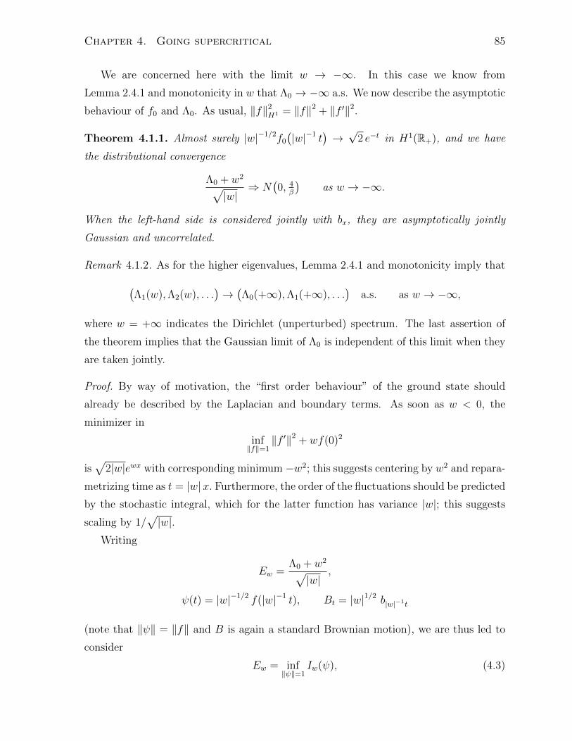
Chapter 4. Going supercritical 85
We are concerned here with the limit w → −∞. In this case we know from
Lemma 2.4.1 and monotonicity in w that Λ0 → −∞ a.s. We now describe the asymptotic
behaviour of f0 and Λ0. As usual, ‖f‖2H1 = ‖f‖2 + ‖f ′‖2.
Theorem 4.1.1. Almost surely |w|−1/2f0(|w|−1 t
)→√
2 e−t in H1(R+), and we have
the distributional convergence
Λ0 + w2√|w|
⇒ N(0, 4
β
)as w → −∞.
When the left-hand side is considered jointly with bx, they are asymptotically jointly
Gaussian and uncorrelated.
Remark 4.1.2. As for the higher eigenvalues, Lemma 2.4.1 and monotonicity imply that(Λ1(w),Λ2(w), . . .
)→(Λ0(+∞),Λ1(+∞), . . .
)a.s. as w → −∞,
where w = +∞ indicates the Dirichlet (unperturbed) spectrum. The last assertion of
the theorem implies that the Gaussian limit of Λ0 is independent of this limit when they
are taken jointly.
Proof. By way of motivation, the “first order behaviour” of the ground state should
already be described by the Laplacian and boundary terms. As soon as w < 0, the
minimizer in
inf‖f‖=1
‖f ′‖2 + wf(0)2
is√
2|w|ewx with corresponding minimum −w2; this suggests centering by w2 and repara-
metrizing time as t = |w|x. Furthermore, the order of the fluctuations should be predicted
by the stochastic integral, which for the latter function has variance |w|; this suggests
scaling by 1/√|w|.
Writing
Ew =Λ0 + w2√|w|
,
ψ(t) = |w|−1/2 f(|w|−1 t), Bt = |w|1/2 b|w|−1t
(note that ‖ψ‖ = ‖f‖ and B is again a standard Brownian motion), we are thus led to
consider
Ew = inf‖ψ‖=1
Iw(ψ), (4.3)
Chapter 4. Going supercritical 86
where the objective quadratic functional is
Iw(ψ) = |w|3/2 J(ψ) + 2√β
∫ ∞0
ψ2 dB + |w|−3/2∫ ∞0
ψ2 t dt (4.4)
in which we put
J(ψ) = ‖ψ′‖2 − ψ(0)2 + ‖ψ‖2 =∥∥ψ′ + ψ
∥∥2.The minimum is attained at
ψw(t) = |w|−1/2 f0(|w|−1 t).
The separation of scales mentioned in the introduction can already be seen in (4.4).
Now on the one hand,
Ew = Iw(ψw) ≥ 2√β
∫ψ2w dB. (4.5)
On the other hand, J(ψ) = 0 for ψ a multiple of e−t; writing
ψ∗(t) =√
2 e−t,
certainly
Ew ≤ Iw(ψ∗) = 2√β
∫ψ2∗ dB + 1
2|w|−3/2 . (4.6)
It is convenient to recouple the models over w so that now paths of B are fixed as w
varies. The proof is completed by Proposition 4.1.5 below, where we show that ψw → ψ∗
as w → −∞ in a sense sufficient to guarantee pathwise convergence of the stochastic
integral in (4.5) to the one in (4.6). Then
Ew → 2√β
∫ψ2∗ dB a.s. as w → −∞, (4.7)
which implies the distributional convergence in the theorem.
As for the joint behaviour with bx, it is enough to show that for s ∈ R and f a
compactly supported step function on R+ we have
E ei(sEw+∫f db) → e−(2/β)s
2−(1/2)‖f‖2 as w → −∞.
Now
E∣∣∣ei(sEw+∫
f db) − ei(s(2/√β)
∫ψ∗dB+
∫f db)
∣∣∣ = E∣∣∣eisEw − eis(2/√β) ∫ ψ∗dB∣∣∣→ 0
Chapter 4. Going supercritical 87
by (4.7) and the bounded convergence theorem. But
E ei(s(2/√β)
∫ψ∗dB+
∫f db) = E ei
∫∞0 (s(2/
√β)ψ∗(t)+|w|−1/2f(|w|−1t))dBt
= e−12
∫∞0 (s(2/
√β)ψ∗(t)+|w|−1/2f(|w|−1t))
2dt
which has the desired limit because the cross term∫∞0ψ∗(t) |w|−1/2f(|w|−1 t) dt → 0.
(The basic fact that L2 functions on distinct scales are asymptotically orthogonal may
be proved by breaking the integral into two pieces on an intermediate scale.)
Lemma 4.1.3. If ψ ∈ H1(R+) with ‖ψ‖L2 = 1 and 〈ψ, ψ∗〉 ≥ 0, then
‖ψ − ψ∗‖2H1 ≤ 8 J(ψ).
Proof. We first claim that for ϕ ∈ H1 with 〈ϕ, e−t〉 = 0 we have
J(ϕ) ≥ ‖ϕ‖2 + 12‖ϕ′‖2 .
Indeed, the orthogonality relation can be integrated by parts to give
ϕ(0) =⟨ϕ′, e−t
⟩;
an application of Cauchy-Schwarz then yields
12‖ϕ′‖2 ≥ ϕ(0)2,
which is equivalent to the claim.
Now put ϕ = ψ − 〈ψ, ψ∗〉ψ∗. By the previous estimate and the hypotheses on ψ,
‖ψ − ψ∗‖2 = 2(1− 〈ψ, ψ∗〉
)≤ 2
(1− 〈ψ, ψ∗〉2
)= 2 ‖ϕ‖2 ≤ 2J(ϕ) = 2J(ψ).
In other words,
‖ψ − ψ∗‖ ≤√
2J(ψ)1/2.
But
J(ψ)1/2 = J(ψ − ψ∗)1/2 = ‖(ψ′ − ψ′∗) + (ψ − ψ∗)‖ ≥ ‖ψ′ − ψ′∗‖ − ‖ψ − ψ∗‖ ,
so also
‖ψ′ − ψ′∗‖ ≤(1 +√
2)J(ψ)1/2.
Square and add to conclude.
Chapter 4. Going supercritical 88
Note that ψw satisfies the hypotheses of this lemma by facts about f0 from Chapter 2.
In particular, ψw > 0 by the oscillation theory (or by Perron-Frobenius theory), so
certainly 〈ψw, ψ∗〉 ≥ 0.
Lemma 4.1.4. There is a random, almost surely finite constant C0 such that∣∣∣∣ 2√β
∫ψ2 dB
∣∣∣∣ ≤ C0
(∥∥ψ′∥∥2 + log(1ε
)∥∥ψ∥∥2 + ε∥∥ψ√t∥∥2) (4.8)
for all ψ and all 0 < ε ≤ 12.
Proof. Decompose B as in RRV (Lemma 2.3 and Proposition 2.4 there); in the last step,
use log(2 + t) ≤ log(1ε
)+ εt. (The function εt + log
(1ε
)− log(2 + t) is minimized at
t = 1ε− 2 with minimum 1− 2ε, so the inequality holds for ε ≤ 1
2.)
It is standard (see e.g. Halmos 1957 §18, Theorem 3) that the above quadratic form
bound may be polarized to a bilinear form bound. Denoting the quantity in parentheses
on the right hand side of (4.8) by ‖ψ‖2L∗ε , we have∣∣∣∣∫ ϕψ dB
∣∣∣∣ ≤ C0
∥∥ϕ∥∥L∗ε
∥∥ψ∥∥L∗ε. (4.9)
Proposition 4.1.5. Almost surely, ψw → ψ∗ in H1(R+) and∫ψ2w dB →
∫ψ2∗ dB.
Proof. Throughout, C denotes a random, almost surely finite constant that is allowed to
change from line to line.
First, using 2 |〈ψ′, ψ〉| ≤ (1− δ) ‖ψ′‖2 + 11−δ ‖ψ‖
2 gives
J(ψ) ≥ δ ‖ψ′‖2 + (1− 11−δ ) ‖ψ‖
2 ≥ δ ‖ψ′‖2 − 2δ ‖ψ‖2
for 0 ≤ δ ≤ 12. Then by (4.6) together with Lemma 4.1.4 (any ε), one has
C ≥ Iw(ψ∗)
≥ Iw(ψw)
≥ |w|3/2(12J(ψw) + (δ/2) ‖ψ′w‖
2 − δ)
+ 2√β
∫ψ2w dB + |w|−3/2
∥∥ψw√t∥∥2.Applying Lemma 4.1.4 now with ε = |w|−3/2 /2C0, and taking δ = 2 |w|−3/2 (C0 + 1)
above, we find
|w|3/2 J(ψw) + ‖ψ′w‖2
+ |w|−3/2∥∥ψw√t∥∥2 ≤ C log |w| (4.10)
Chapter 4. Going supercritical 89
for w sufficiently negative. In particular∥∥ψw − ψ∗∥∥2H1 ≤ 8 J(ψw) ≤ C |w|−3/2 log |w| (4.11)
by Lemma 4.1.3, establishing the first assertion.
We conclude by using (4.9) with ε = |w|−3 as follows:∣∣∣∣∫ (ψ2w − ψ2
∗)dB
∣∣∣∣ ≤ C0
∥∥ψw + ψ∗∥∥L∗ε
∥∥ψw − ψ∗∥∥L∗ε≤ C
(∥∥ψ′w∥∥2 +∥∥ψ′∗∥∥2 + log |w|+ |w|−3
(∥∥ψw√t∥∥2 +∥∥ψ∗√t∥∥2))1/2
×(∥∥ψ′w − ψ′∗∥∥2 + log |w|
∥∥ψw − ψ∗∥∥2 + |w|−3(∥∥ψw√t∥∥2 +
∥∥ψ∗√t∥∥2))1/2≤ C |w|−3/4 log3/2 |w| ,
where the last inequality is a consequence of (4.10) and (4.11).
4.2 The limiting location
Here we focus on the rank one spiked Wishart ensemble and its general β analogue as
defined in Chapter 2. We find the limiting location of the largest eigenvalue using a
simple heuristic together with a little matrix perturbation theory.
Our heuristic is the following observation: A spiked unscaled discrete Laplacian has
a certain geometric sequence as its principal eigenvector, which is decaying in the super-
critical case. Specifically, for r > 0 the matrix
r − 2 1
1 −2 1
1 −2. . .
. . . . . . 1
1 −2 1
1 r−1 − 2
has an eigenvector vi = r−i with corresponding eigenvalue λ = (r− 1)2/r. We know λ is
the top eigenvalue because v has no sign-changes. (The observation also has an infinite
Jacobi matrix version.) The supercritical case is r > 1. In this case we argue that it is
good enough for the matrix to look roughly like this in the top-left corner, which gets us
the limiting location. In the next section we use first-order perturbation theory to give
a heuristic computation of the limiting fluctuations.

Chapter 4. Going supercritical 90
Recall the tridiagonal form Sn,p = W †n,pWn,p with Wn,p = W
β,`n,pn,p as in (2.2). We
recall the following approximations from the heuristics in Section 2.3. The diagonal and
off-diagonal processes of βSn,p are
`n,pχ2βn + χ2
β(p−1), χ2β(n−1) + χ2
β(p−2), χ2β(n−2) + χ2
β(p−3), . . .
χβ(n−1)χβ(p−1), χβ(n−2)χβ(p−2), . . .
respectively. The approximations
χk ≈√k +
√1/2 g, χ2
k ≈ k +√
2k g,
are valid for k large, where g is a suitably coupled standard Gaussian. To leading order,
the top-left corner of S has n+ p on the diagonal and√np on the off-diagonal (ignoring
the spike). So the top-left corner of
1√np
(S −
(√n+√p)2I)
is approximately an unscaled discrete Laplacian.
Theorem 4.2.1. Assuming the notation of Theorem 2.1.1, suppose that√n/p (`n,p − 1) → r > 1 as n ∧ p→∞.
Then in probability (in fact almost surely),
1√np
(λ1 −
(√n+√p)2) → (r − 1)2
ras n ∧ p→∞.
Remark 4.2.2. Of course for all other λk, k ≥ 2 the corresponding limit is zero in this
scaling, by Theorem 2.1.1 and Weyl interlacing.
To recover a statement in the form familiar from Baik and Silverstein (2006), assume
that p/n→ γ2 ∈ (0,∞) and let `n,p = ` = 1 + γr. Our theorem implies the following: If
r > 1, then a.s.1
nλ1 → (1 + γ)2 + γ
(r − 1)2
r= `+ γ2
`
`− 1.
Recall that (1 + γ)2 is the right endpoint of the support of Marcenko-Pastur; the term
γ(r − 1)2/r therefore quantifies the separation. Our formulation treats n and p sym-
metrically (apart from the inherent asymmetry of the spike) and has the advantage of
allowing n, p→∞ together arbitrarily.
Toward a proof, we recall a standard fact.
Chapter 4. Going supercritical 91
Lemma 4.2.3. Let A be a symmetric n×n matrix and endow Rn with the standard inner
product and norm. Suppose that λ ∈ R and v ∈ Rn satisfy ‖v‖ = 1 and∥∥(A− λ)v
∥∥ < ε
for some ε > 0. Then there is an eigenvalue λ of A with∣∣λ− λ∣∣ < ε.
Proof. Let v1, . . . , vn be an orthonormal basis of eigenvalues with corresponding eigen-
vectors λ1, . . . , λn. Write v =∑
i aivi and note that∑
i |ai|2 = 1. Then
ε2 >∥∥(A− λ)v
∥∥2 =∥∥∑
i ai(λi − λ)vi∥∥2 =
∑i
∣∣ai∣∣2∣∣λi − λ∣∣2,which implies that
∣∣λi − λ∣∣2 < ε2 for some i.
Proof of Theorem 4.2.1. Put
An,p =1√np
(Sn,p − (
√n+√p)2)
and rn,p =√n/p (`n,p − 1) .
By the remark and the lemma it suffices to show that∥∥(An,p− λn,p)vn,p
∥∥→ 0 a.s., where
λn,p = (rn,p − 1)2/rn,p and vn,p(i) = r−in,p.
In the following, C denotes a constant that is independent of n, p but may change from
line to line. Let r0 > 1 be such that rn,p ≥ r0 for n ∧ p sufficiently large. Using standard
facts about moments of chi random variables, independence, and that `n,p ≤ C√p/n, we
estimate
E∥∥(A− λ)v
∥∥2 ≤ C
npE
n∧p∑i=0
r−2i0
((pn
+ 1)(
1βχ2β(n−i) − n
)2+(
1βχ2β(p−i) − p
)2+(
1βχβ(n−i)χβ(p−i) −
√np)2)
≤ C
np
n∧p∑i=0
r−2i0
(n+ p+ i(n+ p) + i2(n+ p)
)≤ C
(1
n+
1
p
) ∞∑i=0
i2r−2i0
≤ C
n ∧ p.
(We omitted an additional error of r−(n∧p)0 from the last term.) While this is only good
enough for convergence in probability, similar calculations with higher moments give the
fourth moment bound E∥∥(A− λ)v
∥∥4 ≤ C/(n ∧ p)2.
Chapter 4. Going supercritical 92
4.3 Heuristic for the limiting fluctuations
In the previous section we also predicted the limiting eigenvector. One can therefore
predict the first-order eigenvalue correction, i.e. the fluctuations. First-order perturbation
theory states that if λ, v is an eigenvalue/eigenvector pair of A (with v normalized) and
P is small, then to first order A+ P has an eigenvalue λ+ v†Pv.
We take up the approximations of the previous section. To first order, we found that(Sn,p − (
√n+√p)2)/√np is a “spiked discrete Laplacian”. The next order terms are,
omitting a√
2/β prefactor and going down the diagonal and off-diagonal respectively:
1√p`gn + 1√
ngp−1,
1√pgn−1 + 1√
ngp−2,
1√pgn−2 + 1√
ngp−3, . . .
12√ngn−1 + 1
2√pgp−1,
12√ngn−2 + 1
2√pgp−2, . . .
where we have labeled the g’s to match the corresponding χ’s, the important thing
being that distinctly labeled g’s are independent. Again with rn,p =√n/p (`n,p − 1), the
limiting eigenvector is√
1− r−2[
1 r−1 r−2 . . .]†.
First order perturbation theory then predicts that(λ1 − (
√n+√p)2)/√np has Gaussian
fluctuations with variance
2β(1− r−2)2
(1p`2 + ( 1√
n+ 1√
pr−1)2 + ( 1√
nr−1 + 1√
pr−2)2 + · · ·
)= 2
β(1− r−2)
(1p`2(1− r−2) + ( 1√
n+ 1√
pr−1)2
)= 2
β(1− r−2)
(1p`2(1− p
n(`−1)2)
+ 1n
(``−1
)2)=
2
β
(`2
p− `2
n(`− 1)2
).
This prediction agrees with results of BBP, Paul (2007) for β = 1, 2 respectively.
Note once again that we state the scaling slightly differently, dividing λ1 by√np rather
than n; our formulation has the advantage of symmetry in n, p and allowing n, p → ∞arbitrarily.
Chapter 5
Connection with Painleve II
In this chapter we connect our PDE characterization of the deformed Tracy-Widom(β)
laws, Theorems 2.1.7(ii), 2.4.3 and 3.1.6, with known Painleve II representations for these
laws at β = 2 due to Baik (2006) (derived of course from the Fredholm determinant
representations of BBP). In the rank one case we obtain a rigorous alternative proof
of these representations. Furthermore, using results of Baik and Rains (2000, 2001) we
guess and prove a similar formula at β = 4. In particular, we recover a novel proof of
the Painleve II representations of the Tracy-Widom laws for β = 2, 4.
At β = 2 we indicate how the connection extends to the second largest and subsequent
eigenvalue laws. Put another way, the connection between the PDE and Painleve II
includes not only the Hastings-McLeod solution but also the Ablowitz-Segur solutions.
For the multi-spiked deformations, we describe a computer-assisted symbolic computation
providing strong evidence that the connection holds here as well.
A number of points remain somewhat mysterious. Most obviously, we lack a connec-
tion in the β = 1 case; while the literature previously did not even suggest a guess, it
would now be satisfying to reconcile (2.9), (2.10) with the formula obtained by Mo (2011).
We point out that in the work of Dieng (2005), the β = 1 case also involves additional
complications; perhaps they are related to ours, though this is idle speculation.
Even at β = 2, 4 it seems there should be a more direct way to derive or at least
understand the connection. From the point of view of the PDE, some kind of extra
structure appears to be present at certain special values of the parameter β; what about
other values? From the point of view of nonlinear special functions, we show directly—
independently of any limit theorems—how certain well-studied solutions of Painleve II
admit a new characterization in terms of a linear parabolic boundary value problem in
93
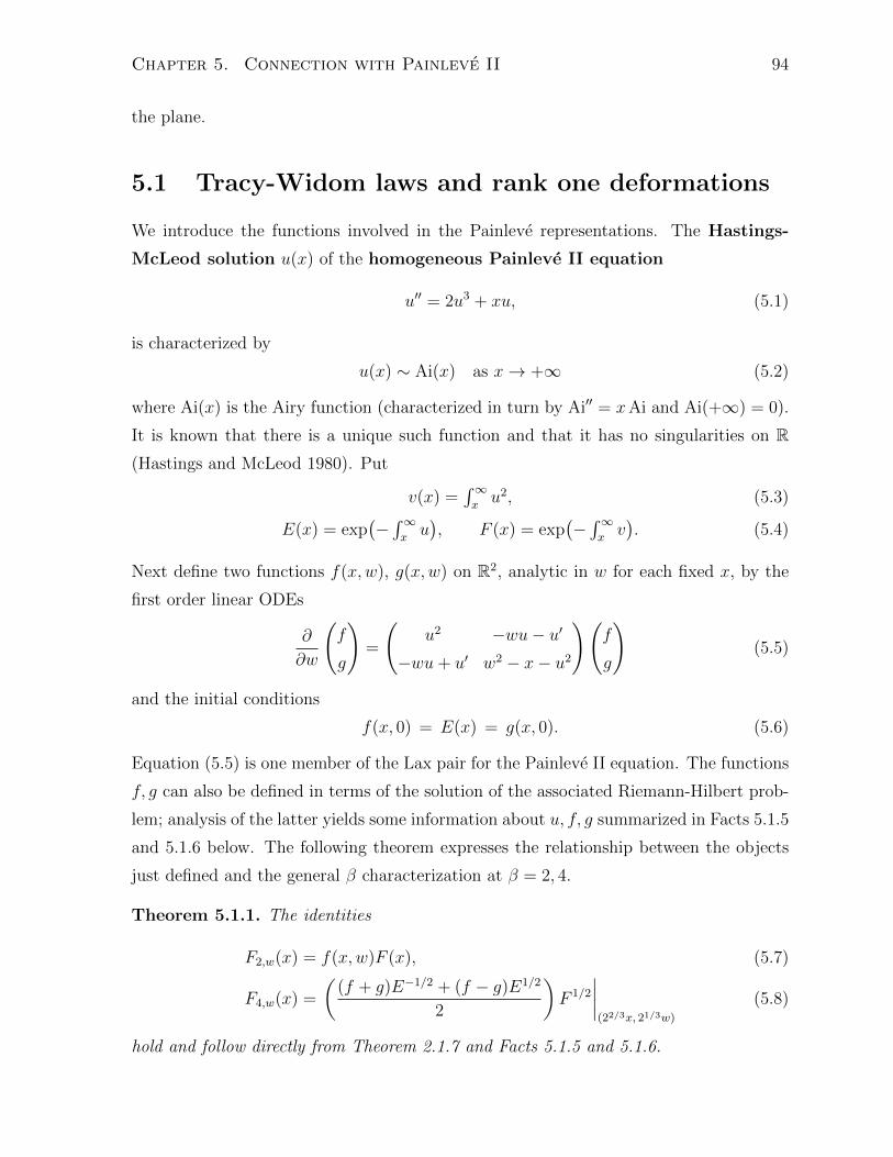
Chapter 5. Connection with Painleve II 94
the plane.
5.1 Tracy-Widom laws and rank one deformations
We introduce the functions involved in the Painleve representations. The Hastings-
McLeod solution u(x) of the homogeneous Painleve II equation
u′′ = 2u3 + xu, (5.1)
is characterized by
u(x) ∼ Ai(x) as x→ +∞ (5.2)
where Ai(x) is the Airy function (characterized in turn by Ai′′ = xAi and Ai(+∞) = 0).
It is known that there is a unique such function and that it has no singularities on R(Hastings and McLeod 1980). Put
v(x) =∫∞xu2, (5.3)
E(x) = exp(−∫∞xu), F (x) = exp
(−∫∞xv). (5.4)
Next define two functions f(x,w), g(x,w) on R2, analytic in w for each fixed x, by the
first order linear ODEs
∂
∂w
(f
g
)=
(u2 −wu− u′
−wu+ u′ w2 − x− u2
)(f
g
)(5.5)
and the initial conditions
f(x, 0) = E(x) = g(x, 0). (5.6)
Equation (5.5) is one member of the Lax pair for the Painleve II equation. The functions
f, g can also be defined in terms of the solution of the associated Riemann-Hilbert prob-
lem; analysis of the latter yields some information about u, f, g summarized in Facts 5.1.5
and 5.1.6 below. The following theorem expresses the relationship between the objects
just defined and the general β characterization at β = 2, 4.
Theorem 5.1.1. The identities
F2,w(x) = f(x,w)F (x), (5.7)
F4,w(x) =
((f + g)E−1/2 + (f − g)E1/2
2
)F 1/2
∣∣∣∣(22/3x, 21/3w)
(5.8)
hold and follow directly from Theorem 2.1.7 and Facts 5.1.5 and 5.1.6.
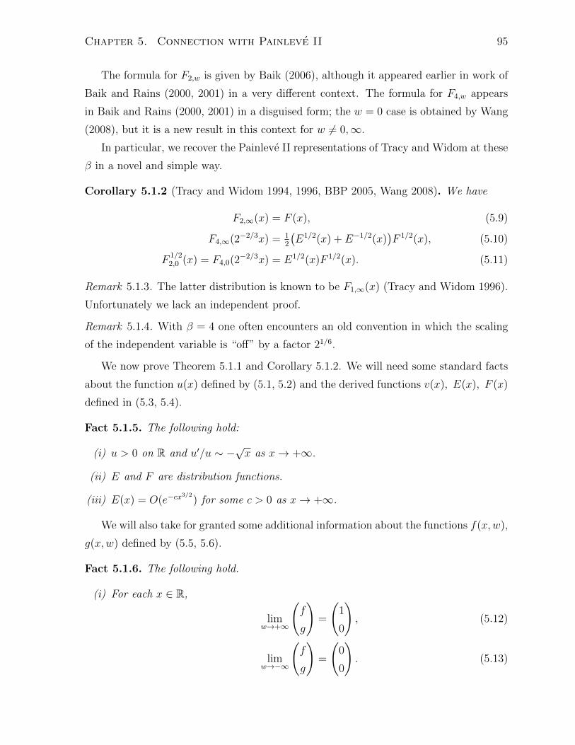
Chapter 5. Connection with Painleve II 95
The formula for F2,w is given by Baik (2006), although it appeared earlier in work of
Baik and Rains (2000, 2001) in a very different context. The formula for F4,w appears
in Baik and Rains (2000, 2001) in a disguised form; the w = 0 case is obtained by Wang
(2008), but it is a new result in this context for w 6= 0,∞.
In particular, we recover the Painleve II representations of Tracy and Widom at these
β in a novel and simple way.
Corollary 5.1.2 (Tracy and Widom 1994, 1996, BBP 2005, Wang 2008). We have
F2,∞(x) = F (x), (5.9)
F4,∞(2−2/3x) = 12
(E1/2(x) + E−1/2(x)
)F 1/2(x), (5.10)
F1/22,0 (x) = F4,0(2
−2/3x) = E1/2(x)F 1/2(x). (5.11)
Remark 5.1.3. The latter distribution is known to be F1,∞(x) (Tracy and Widom 1996).
Unfortunately we lack an independent proof.
Remark 5.1.4. With β = 4 one often encounters an old convention in which the scaling
of the independent variable is “off” by a factor 21/6.
We now prove Theorem 5.1.1 and Corollary 5.1.2. We will need some standard facts
about the function u(x) defined by (5.1, 5.2) and the derived functions v(x), E(x), F (x)
defined in (5.3, 5.4).
Fact 5.1.5. The following hold:
(i) u > 0 on R and u′/u ∼ −√x as x→ +∞.
(ii) E and F are distribution functions.
(iii) E(x) = O(e−cx3/2
) for some c > 0 as x→ +∞.
We will also take for granted some additional information about the functions f(x,w),
g(x,w) defined by (5.5, 5.6).
Fact 5.1.6. The following hold.
(i) For each x ∈ R,
limw→+∞
(f
g
)=
(1
0
), (5.12)
limw→−∞
(f
g
)=
(0
0
). (5.13)
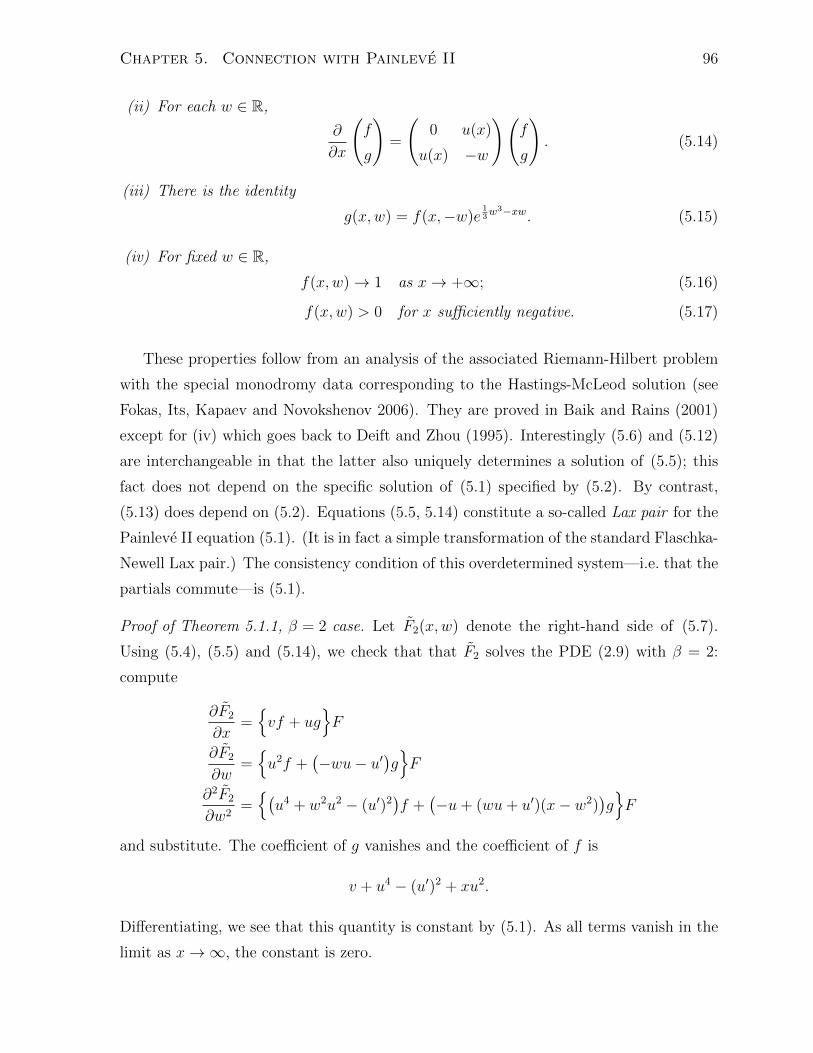
Chapter 5. Connection with Painleve II 96
(ii) For each w ∈ R,
∂
∂x
(f
g
)=
(0 u(x)
u(x) −w
)(f
g
). (5.14)
(iii) There is the identity
g(x,w) = f(x,−w)e13w3−xw. (5.15)
(iv) For fixed w ∈ R,
f(x,w)→ 1 as x→ +∞; (5.16)
f(x,w) > 0 for x sufficiently negative. (5.17)
These properties follow from an analysis of the associated Riemann-Hilbert problem
with the special monodromy data corresponding to the Hastings-McLeod solution (see
Fokas, Its, Kapaev and Novokshenov 2006). They are proved in Baik and Rains (2001)
except for (iv) which goes back to Deift and Zhou (1995). Interestingly (5.6) and (5.12)
are interchangeable in that the latter also uniquely determines a solution of (5.5); this
fact does not depend on the specific solution of (5.1) specified by (5.2). By contrast,
(5.13) does depend on (5.2). Equations (5.5, 5.14) constitute a so-called Lax pair for the
Painleve II equation (5.1). (It is in fact a simple transformation of the standard Flaschka-
Newell Lax pair.) The consistency condition of this overdetermined system—i.e. that the
partials commute—is (5.1).
Proof of Theorem 5.1.1, β = 2 case. Let F2(x,w) denote the right-hand side of (5.7).
Using (5.4), (5.5) and (5.14), we check that that F2 solves the PDE (2.9) with β = 2:
compute
∂F2
∂x={vf + ug
}F
∂F2
∂w={u2f +
(−wu− u′
)g}F
∂2F2
∂w2={(u4 + w2u2 − (u′)2
)f +
(−u+ (wu+ u′)(x− w2)
)g}F
and substitute. The coefficient of g vanishes and the coefficient of f is
v + u4 − (u′)2 + xu2.
Differentiating, we see that this quantity is constant by (5.1). As all terms vanish in the
limit as x→∞, the constant is zero.
Chapter 5. Connection with Painleve II 97
We must check that F2 is bounded and that it has the boundary behaviour (2.10).
To this end we claim f, g > 0 on R2. Fixing w, (5.17, 5.15) cover x sufficiently negative.
Now (5.14) shows f increases at least until x0 = min{x : g(x,w) = 0}. But if x0
exists then (5.14) shows ∂g∂x
(x0) > 0, a contradiction. This proves the claim. It now
follows from (5.14) that ∂f∂x
> 0. From (5.16) we deduce that f ≤ 1; in particular f is
bounded, and hence so is F2. Furthermore, for a given x ∈ R and ε > 0, (5.12) yields
w+ such that f > 1 − ε on [x,∞) × [w+,∞), and (5.13) yields w− such that f < ε on
(−∞, x]× (−∞, w−]. Using that F (x) is a distribution function, (2.10) follows.
Proof of Theorem 5.1.1, β = 4 case. That the right-hand side F4 of (5.8) satisfies the
PDE (2.9) with β = 4 may be verified just as in the β = 2 case; the computation is more
tedious but the result is very similar and the final step is the same.
It is a little more work to get boundedness and the boundary behaviour (2.10) this
time. Dropping the scale factors on x,w, consider
G = F−1/2F4 = 12
(E−1/2 + E1/2
)f + 1
2
(E−1/2 − E1/2
)g.
Clearly G > 0. For fixed w, G→ 1 as x→∞ by (5.16) and the fact that E−1/2−E1/2 =
O(e−cx3/2
) while g = O(ewx) from (5.15). Now by (5.14) we have
∂G
∂x= 1
2
(E−1/2 + E1/2
)(12ug)
+ 12
(E−1/2 − E1/2
)(12uf − wg
),
which is positive for w ≤ 0. Boundedness in the lower half-plane {w ≤ 0} follows, as
does the lower boundary behaviour using (5.13).
From (5.15) we immediately see g ≤ 1 on {x ≥ 0, 0 ≤ w ≤√
3x}. By Lemma 5.1.2,∂∂wFβ,w(x) ≥ 0. The β = 2 case of the present theorem then implies that ∂f
∂w≥ 0.
From (5.5) we conclude g ≤ u/(w + u′/u) provided the denominator is positive. But
u′/u ∼ −√x as x → +∞, so there is x1 such that u′/u ≥ −
√2x for x ≥ x1. The latter
bound for g therefore implies that g is bounded on {x ≥ x1, w ≥√
3x}. Moreover, for
any x0 < x1 we have that u and u′/u are bounded on the interval x0 ≤ x ≤ x1, so
g is bounded uniformly over these x for all w sufficiently large. Putting these bounds
together we conclude g is bounded on all right half-planes {x ≥ x0}, and the same then
follows for F4.
The upper boundary behaviour follows as well. Indeed, as x,w → ∞ together the
coefficient of g vanishes while the coefficient of f tends to 1; the g-term then vanishes
while the f -term tends to 1 as in the β = 2 case.
Chapter 5. Connection with Painleve II 98
It remains to show F4 is bounded on the whole plane; it suffices to bound F4 on the
upper-left quadrant Q = {x ≤ 0, w ≥ 0}. Here we can use the fact that F4 solves the
PDE. With notation as in Theorem 2.1.7 we have that F4(x, px) is a local martingale under
P(x0,w0). By boundedness on right half-planes, it is in fact a bounded martingale. Using
that paths explode only to −∞, optional stopping gives the representation F4(x0, w0) =
E(x0,w0) F4(T, pT ) where T = inf{x : (x, px) /∈ Q}. The bound thus extends to Q.
Proof of Corollary 5.1.2. These identities are straightforward consequences of the theo-
rem, (5.6) and (5.12).
5.2 Subsequent eigenvalue laws
In the previous section we demonstrated an explicit connection between our boundary
value problem for the top eigenvalue law at β = 2 and the Hastings-McLeod solution of
Painleve II. In this section, based on conversations with Alexander Its, we outline how
the connection extends to one between the boundary value problem for the subsequent
eigenvalue laws and the Ablowitz-Segur solutions.
Taking up the notation of Theorem 2.4.3, let F(k)(x;w) and F(k)(x) = F(k)(x; +∞) be
the limiting distributions for the w-deformed and un-deformed (k+1)st largest eigenvalue
with β = 2. Suppose 0 ≤ λ ≤ 1. Tracy and Widom (1994) proved that
∞∑k=0
(1− λ)kλF(k)(x) = exp
(−∫ ∞x
(s− x)u2(s, λ) ds
)(5.18)
where u(·, λ) solves (5.1) subject to
u(x, λ) ∼√λAi(x) as x→∞. (5.19)
Ablowitz and Segur (1977) show that the latter function is unique with no singularities
on R for 0 ≤ λ < 1; Hastings and McLeod (1980) showed this statement continues
to hold for λ = 1 (but fails for λ > 1). The subsequent eigenvalue laws are therefore
expressed, via the generating function on the left side of (5.18), in terms of the Ablowitz-
Segur solutions. Of course one could differentiate repeatedly at λ = 1 and solve for
F(1), F(2), . . . to obtain the formulas in Tracy and Widom (1994).
Remark 5.2.1. Tracy and Widom (1994) actually showed the two sides of (5.18) are
both equal to a certain Fredholm determinant. We briefly explain the situation by
Chapter 5. Connection with Painleve II 99
introducing the determinantal representation at β = 2; while not neeeded here, it is
somewhat illuminating. The β = 2 soft edge limit is a determinantal point process with
the so-called Airy kernel given by
A(x, y) =Ai(x) Ai′(y)− Ai′(x) Ai(y)
x− y
(Forrester 1993). See Hough, Krishnapur, Peres and Virag (2009) for definitions and facts
about determinantal processes. The gap probabilities can be represented by Fredholm
determinants: for example,
F(0)(x) = det(1−Ax)
where Ax represents the (trace class) integral operator with Airy kernel acting on
L2(x,∞). The subsequent eigenvalue laws are encoded as follows. For 0 ≤ λ ≤ 1,
the determinantal process with kernel λAx can be described probabilistically by sam-
pling from the original λ = 1 process and then independently deleting each point with
probability 1 − λ. For the gap probability of this “incomplete spectrum” we then have
the geometric mixture
∞∑k=0
(1− λ)kλF(k)(x) = det(1− λAx). (5.20)
Tracy and Widom (1994) prove the identity of the right hand sides of (5.18) and (5.20).
Turning to our PDE characterization Theorem 2.4.3, consider the geometric mixture
Fλ(x;w) =∞∑k=0
(1− λ)kλF(k)(x;w).
Recall that F(k) solves the usual PDE (2.9); by linearity, so does Fλ. Writing the boundary
conditions informally, F(k) also solves the usual F(k)(+∞,+∞) = 1 but now the recursive
condition
F(k)(x,−∞) = F(k−1)(x,+∞).
It follows that Fλ solves Fλ(+∞,+∞) = 1 but now the “periodic” condition
Fλ(x,−∞) = (1− λ)Fλ(x,+∞). (5.21)
One can show that there is a unique bounded solution of the PDE with these boundary
conditions; argue as in Section 2.4 but using a diffusion path that explodes and restarts
a random number of times with Geometric(λ) distribution.
Chapter 5. Connection with Painleve II 100
Now, one can also define λ-dependent “Ablowitz-Segur versions” of v(x), E(x), F (x),
f(x;w), g(x;w) by (5.3)–(5.6) but using u(x, λ) characterized by (5.1),(5.19). Once again
(5.14) also holds, and therefore Fλ(x;w) = F (x)f(x,w) satisfies the PDE (2.9) by the
same independent verification as in Section 5.1. Remarkably, it is also possible to verify
independently that this f and hence Fλ satisfy the same boundary conditions as those
satisfied by Fλ, especially the periodic boundary conditon (5.21)! We omit the details,
deferring to a personal communication (Its 2011).
5.3 Higher-rank deformations
Baik (2006) also gives a formula for the multi-parameter function F2(x;w1, . . . , wr) which
appeared originally in BBP and which we also characterize in Theorem 3.1.6. While we
do not have an independent proof of Baik’s formula at present, we used the computer
algebra system Maple to verify symbolically that it does indeed satisfy our PDE (3.6) at
β = 2 for r = 2, 3, 4, 5. Of course, a pencil-and-paper proof for all r would be much more
satisfying. (It would then remain to verify boundedness and the boundary conditions
(3.7),(3.8).)
Baik’s formula is
F2(x;w1, . . . , wr) = F (x)det((wi + ∂
∂x
)j−1f(x,wi)
)1≤i,j≤r∏
1≤i<j≤r(wj − wi). (5.22)
Our symbolic verification for small values of r consisted of the following steps. The
differential relations given by (5.1), (5.3), (5.4), (5.5) and (5.14) were encoded as formal
substitution rules. The determinant in (5.22) was expanded (this step becomes problem-
atic for larger r!) and the result plugged into our PDE (3.6). The substitution rules were
then applied repeatedly. Finally, the result was factored using Maple’s built-in command.
Each time, the output contained the factor
v + u4 − (u′)2 + xu2,
which vanishes identically. (Once again, differentiate and apply (5.1) to see it is constant
and then take x→∞ to see the constant is zero.)
Chapter 6
A note on numerics
Consider the problem of evaluating the Tracy-Widom distributions Fβ(x) numerically.
One use for such values (especially with β = 1) is in hypothesis testing on high-
dimensional data, e.g. with the so-called largest root test (Johnstone 2001, 2007, 2008,
2009). Another use has been in high-precision experimental verification of mathematical
predictions about growth interface fluctuations (Takeuchi and Sano 2010). A third use
is in “experimental mathematics”: good numerics allow one to test proposed relations
or identities before attempting a proof, and even sometimes to discover new identities
(Bornemann 2010a).
If there were no structure at all, the only recourse would be to Monte Carlo simu-
lation with large random matrices. Of course, the Fredholm determinant and Painleve
II representations suggest better alternatives. For a long time, the common point of
view was that the Painleve representations offered the most straightforward method. As
this method essentially only requires solving an ODE/initial value problem on the line,
one might reasonably expect this to be the case. Unfortunately, naıve solution of the
Painleve II equation (5.1) with Hastings-Mcleod asymptotic data (5.2) is well-known to
be unstable and inevitably leads to large errors. Deeper knowledge of this nonlinear
special function (the so-called “connection formulas” giving the left tail asymptotics)
allowed Tracy and Widom and especially Prahofer and Spohn (2004) to obtain good re-
sults. The latter authors obtained tables with 16-digit accuracy (Prahofer 2003) but used
variable precision software arithmetic with up to 1500 digits. More recently, Bornemann
(2010b) demonstrated that the Fredholm determinant representations actually offer the
better route to efficient and accurate numerical evaluation. See Bornemann (2010a) for
a review of these developments.
101
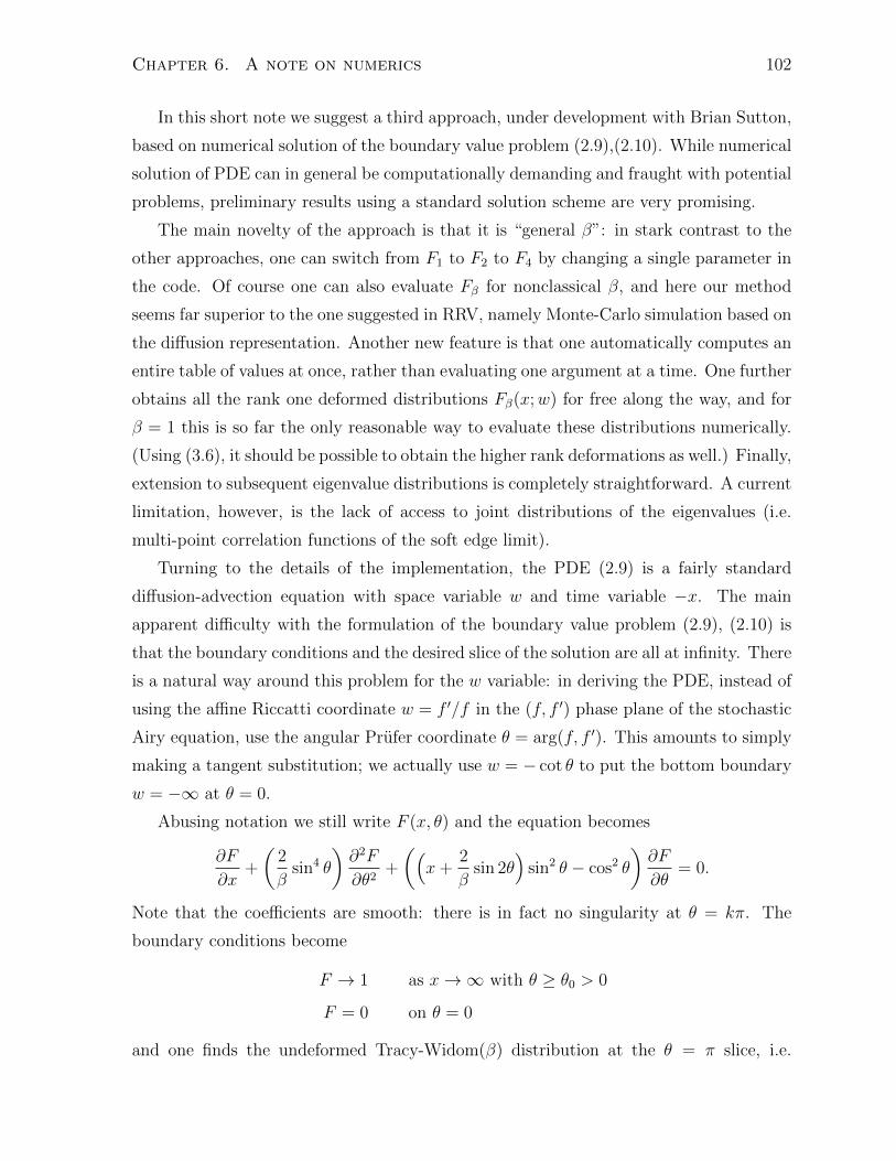
Chapter 6. A note on numerics 102
In this short note we suggest a third approach, under development with Brian Sutton,
based on numerical solution of the boundary value problem (2.9),(2.10). While numerical
solution of PDE can in general be computationally demanding and fraught with potential
problems, preliminary results using a standard solution scheme are very promising.
The main novelty of the approach is that it is “general β”: in stark contrast to the
other approaches, one can switch from F1 to F2 to F4 by changing a single parameter in
the code. Of course one can also evaluate Fβ for nonclassical β, and here our method
seems far superior to the one suggested in RRV, namely Monte-Carlo simulation based on
the diffusion representation. Another new feature is that one automatically computes an
entire table of values at once, rather than evaluating one argument at a time. One further
obtains all the rank one deformed distributions Fβ(x;w) for free along the way, and for
β = 1 this is so far the only reasonable way to evaluate these distributions numerically.
(Using (3.6), it should be possible to obtain the higher rank deformations as well.) Finally,
extension to subsequent eigenvalue distributions is completely straightforward. A current
limitation, however, is the lack of access to joint distributions of the eigenvalues (i.e.
multi-point correlation functions of the soft edge limit).
Turning to the details of the implementation, the PDE (2.9) is a fairly standard
diffusion-advection equation with space variable w and time variable −x. The main
apparent difficulty with the formulation of the boundary value problem (2.9), (2.10) is
that the boundary conditions and the desired slice of the solution are all at infinity. There
is a natural way around this problem for the w variable: in deriving the PDE, instead of
using the affine Riccatti coordinate w = f ′/f in the (f, f ′) phase plane of the stochastic
Airy equation, use the angular Prufer coordinate θ = arg(f, f ′). This amounts to simply
making a tangent substitution; we actually use w = − cot θ to put the bottom boundary
w = −∞ at θ = 0.
Abusing notation we still write F (x, θ) and the equation becomes
∂F
∂x+
(2
βsin4 θ
)∂2F
∂θ2+
((x+
2
βsin 2θ
)sin2 θ − cos2 θ
)∂F
∂θ= 0.
Note that the coefficients are smooth: there is in fact no singularity at θ = kπ. The
boundary conditions become
F → 1 as x→∞ with θ ≥ θ0 > 0
F = 0 on θ = 0
and one finds the undeformed Tracy-Widom(β) distribution at the θ = π slice, i.e.
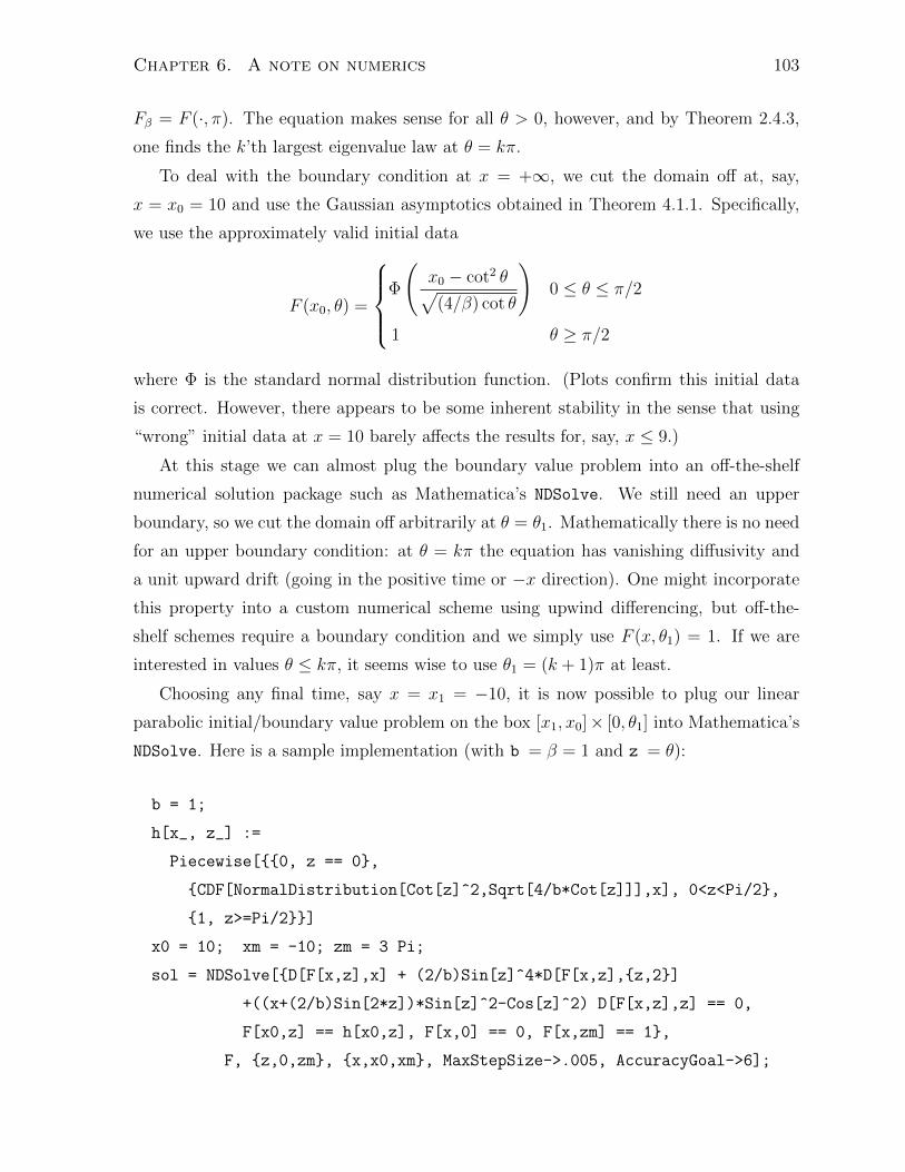
Chapter 6. A note on numerics 103
Fβ = F (·, π). The equation makes sense for all θ > 0, however, and by Theorem 2.4.3,
one finds the k’th largest eigenvalue law at θ = kπ.
To deal with the boundary condition at x = +∞, we cut the domain off at, say,
x = x0 = 10 and use the Gaussian asymptotics obtained in Theorem 4.1.1. Specifically,
we use the approximately valid initial data
F (x0, θ) =
Φ
(x0 − cot2 θ√(4/β) cot θ
)0 ≤ θ ≤ π/2
1 θ ≥ π/2
where Φ is the standard normal distribution function. (Plots confirm this initial data
is correct. However, there appears to be some inherent stability in the sense that using
“wrong” initial data at x = 10 barely affects the results for, say, x ≤ 9.)
At this stage we can almost plug the boundary value problem into an off-the-shelf
numerical solution package such as Mathematica’s NDSolve. We still need an upper
boundary, so we cut the domain off arbitrarily at θ = θ1. Mathematically there is no need
for an upper boundary condition: at θ = kπ the equation has vanishing diffusivity and
a unit upward drift (going in the positive time or −x direction). One might incorporate
this property into a custom numerical scheme using upwind differencing, but off-the-
shelf schemes require a boundary condition and we simply use F (x, θ1) = 1. If we are
interested in values θ ≤ kπ, it seems wise to use θ1 = (k + 1)π at least.
Choosing any final time, say x = x1 = −10, it is now possible to plug our linear
parabolic initial/boundary value problem on the box [x1, x0]× [0, θ1] into Mathematica’s
NDSolve. Here is a sample implementation (with b = β = 1 and z = θ):
b = 1;
h[x_, z_] :=
Piecewise[{{0, z == 0},
{CDF[NormalDistribution[Cot[z]^2,Sqrt[4/b*Cot[z]]],x], 0<z<Pi/2},
{1, z>=Pi/2}}]
x0 = 10; xm = -10; zm = 3 Pi;
sol = NDSolve[{D[F[x,z],x] + (2/b)Sin[z]^4*D[F[x,z],{z,2}]
+((x+(2/b)Sin[2*z])*Sin[z]^2-Cos[z]^2) D[F[x,z],z] == 0,
F[x0,z] == h[x0,z], F[x,0] == 0, F[x,zm] == 1},
F, {z,0,zm}, {x,x0,xm}, MaxStepSize->.005, AccuracyGoal->6];
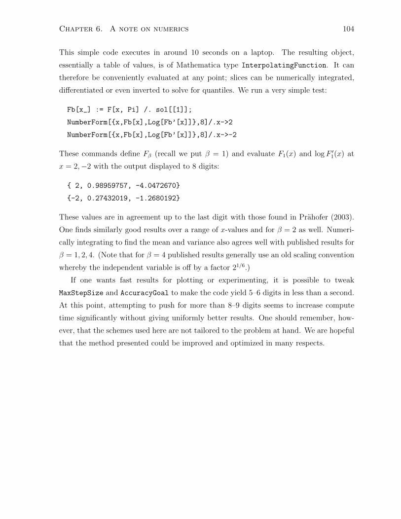
Chapter 6. A note on numerics 104
This simple code executes in around 10 seconds on a laptop. The resulting object,
essentially a table of values, is of Mathematica type InterpolatingFunction. It can
therefore be conveniently evaluated at any point; slices can be numerically integrated,
differentiated or even inverted to solve for quantiles. We run a very simple test:
Fb[x_] := F[x, Pi] /. sol[[1]];
NumberForm[{x,Fb[x],Log[Fb’[x]]},8]/.x->2
NumberForm[{x,Fb[x],Log[Fb’[x]]},8]/.x->-2
These commands define Fβ (recall we put β = 1) and evaluate F1(x) and logF ′1(x) at
x = 2,−2 with the output displayed to 8 digits:
{ 2, 0.98959757, -4.0472670}
{-2, 0.27432019, -1.2680192}
These values are in agreement up to the last digit with those found in Prahofer (2003).
One finds similarly good results over a range of x-values and for β = 2 as well. Numeri-
cally integrating to find the mean and variance also agrees well with published results for
β = 1, 2, 4. (Note that for β = 4 published results generally use an old scaling convention
whereby the independent variable is off by a factor 21/6.)
If one wants fast results for plotting or experimenting, it is possible to tweak
MaxStepSize and AccuracyGoal to make the code yield 5–6 digits in less than a second.
At this point, attempting to push for more than 8–9 digits seems to increase compute
time significantly without giving uniformly better results. One should remember, how-
ever, that the schemes used here are not tailored to the problem at hand. We are hopeful
that the method presented could be improved and optimized in many respects.
Appendix A
Stochastic Airy is a classical
Sturm-Liouville problem
The spectral theory of the Stochastic Airy operator and its Riccati diffusion representa-
tion are developed in Ramırez, Rider and Virag (2011) (RRV). It is possible to recast
this development to take advantage of classical Sturm-Liouville theory. The point is
that continuous integrated potentials actually fall well within the scope of the standard
theory. One rewrites the eigenvalue equation as a pair of first order linear ODEs with
continuous coefficients; this system is in fact equivalent to the integrated form of the
eigenvalue equation in the paper. A further change of variables reduces the equation to
standard Sturm-Liouville form with coefficients satisfying the most classical hypotheses.
The main advantage is that various standard results become available. For the prob-
lem on a finite interval, the classical Sturm oscillation and comparison theorems apply
directly. One also more easily gets a full picture of the spectral theory, including for
example the completeness of the eigenfunctions in L2(R+).
After the fact, one can apply the Riccati transformation to the linear system, obtain-
ing a nonlinear ODE with continuous coefficients whose solutions are already understood.
A final change of variables recovers the SDE from the ODE. This formulation has the
further advantage of avoiding infinity: “blowups and restarts” only appear once the work
is already done. Of course, they could be avoided altogether by working with the angular
Prufer coordinate instead of the affine Riccati coordinate in the phase plane; the resulting
ODE and SDE have trigonometric rather than quadratic nonlinearity, however, and are
somewhat more complicated (see Chapter 6).
105
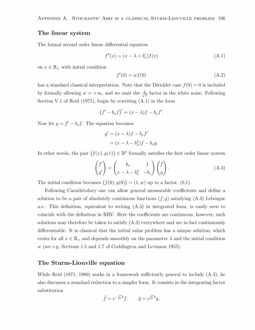
Appendix A. Stochastic Airy is a classical Sturm-Liouville problem 106
The linear system
The formal second order linear differential equation
f ′′(x) = (x− λ+ b′x)f(x) (A.1)
on x ∈ R+ with initial condition
f ′(0) = wf(0) (A.2)
has a standard classical interpretation. Note that the Dirichlet case f(0) = 0 is included
by formally allowing w = +∞, and we omit the 2√β
factor in the white noise. Following
Section V.1 of Reid (1971), begin by rewriting (A.1) in the form(f ′ − bxf
)′= (x− λ)f − bxf ′.
Now let g = f ′ − bxf . The equation becomes
g′ = (x− λ)f − bxf ′
= (x− λ− b2x)f − bxg.
In other words, the pair(f(x), g(x)
)∈ R2 formally satisfies the first order linear system(
f ′
g′
)=
(bx 1
x− λ− b2x −bx
)(f
g
). (A.3)
The initial condition becomes(f(0), g(0)
)= (1, w) up to a factor, (0,1).
Following Caratheodory one can allow general measurable coefficients and define a
solution to be a pair of absolutely continuous functions (f, g) satisfying (A.3) Lebesgue
a.e. This definition, equivalent to writing (A.3) in integrated form, is easily seen to
coincide with the definition in RRV. Here the coefficients are continuous, however; such
solutions may therefore be taken to satisfy (A.3) everywhere and are in fact continuously
differentiable. It is classical that the initial value problem has a unique solution, which
exists for all x ∈ R+ and depends smoothly on the parameter λ and the initial condition
w (see e.g. Sections 1.5 and 1.7 of Coddington and Levinson 1955).
The Sturm-Liouville equation
While Reid (1971, 1980) works in a framework sufficiently general to include (A.3), he
also discusses a standard reduction to a simpler form. It consists in the integrating factor
substitution
f = e−∫ x0 bf, g = e
∫ x0 bg,
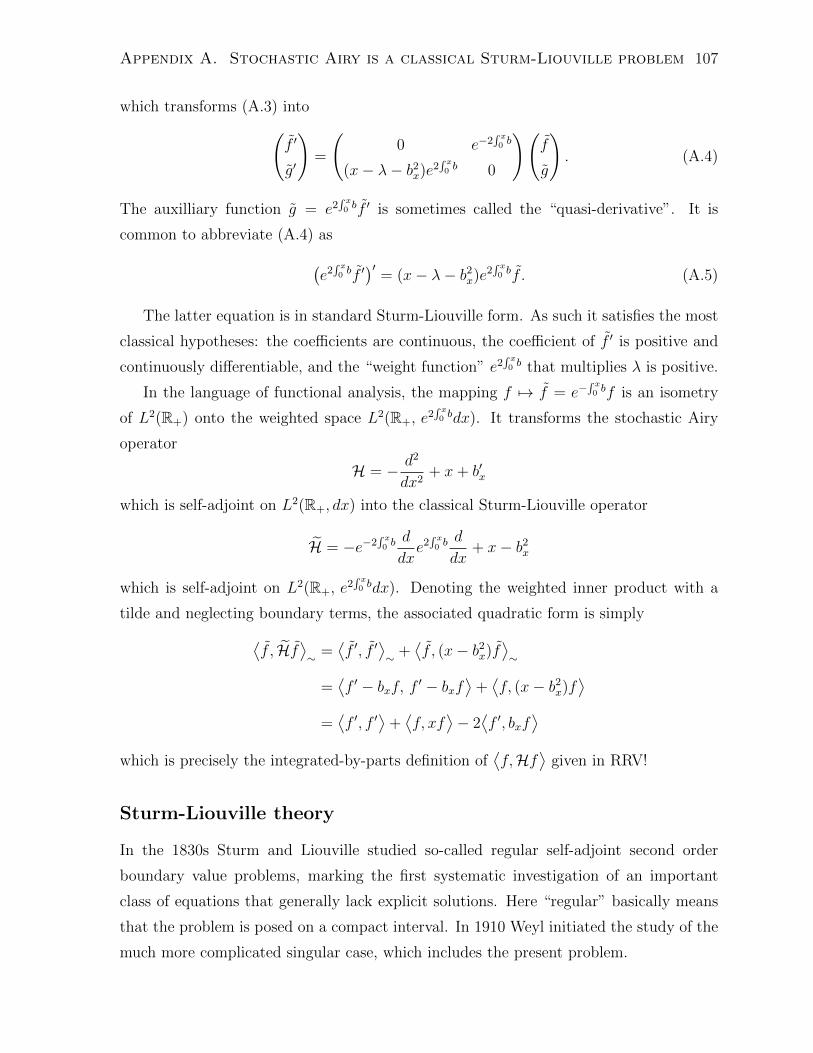
Appendix A. Stochastic Airy is a classical Sturm-Liouville problem 107
which transforms (A.3) into(f ′
g′
)=
(0 e−2
∫ x0 b
(x− λ− b2x)e2∫ x0 b 0
)(f
g
). (A.4)
The auxilliary function g = e2∫ x0 bf ′ is sometimes called the “quasi-derivative”. It is
common to abbreviate (A.4) as(e2
∫ x0 bf ′
)′= (x− λ− b2x)e2
∫ x0 bf . (A.5)
The latter equation is in standard Sturm-Liouville form. As such it satisfies the most
classical hypotheses: the coefficients are continuous, the coefficient of f ′ is positive and
continuously differentiable, and the “weight function” e2∫ x0 b that multiplies λ is positive.
In the language of functional analysis, the mapping f 7→ f = e−∫ x0 bf is an isometry
of L2(R+) onto the weighted space L2(R+, e2∫ x0 bdx). It transforms the stochastic Airy
operator
H = − d2
dx2+ x+ b′x
which is self-adjoint on L2(R+, dx) into the classical Sturm-Liouville operator
H = −e−2∫ x0 bd
dxe2
∫ x0 bd
dx+ x− b2x
which is self-adjoint on L2(R+, e2∫ x0 bdx). Denoting the weighted inner product with a
tilde and neglecting boundary terms, the associated quadratic form is simply⟨f , Hf
⟩∼ =
⟨f ′, f ′
⟩∼ +
⟨f , (x− b2x)f
⟩∼
=⟨f ′ − bxf, f ′ − bxf
⟩+⟨f, (x− b2x)f
⟩=⟨f ′, f ′
⟩+⟨f, xf
⟩− 2⟨f ′, bxf
⟩which is precisely the integrated-by-parts definition of
⟨f,Hf
⟩given in RRV!
Sturm-Liouville theory
In the 1830s Sturm and Liouville studied so-called regular self-adjoint second order
boundary value problems, marking the first systematic investigation of an important
class of equations that generally lack explicit solutions. Here “regular” basically means
that the problem is posed on a compact interval. In 1910 Weyl initiated the study of the
much more complicated singular case, which includes the present problem.
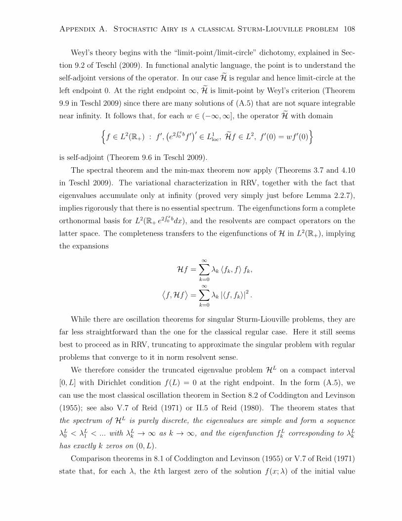
Appendix A. Stochastic Airy is a classical Sturm-Liouville problem 108
Weyl’s theory begins with the “limit-point/limit-circle” dichotomy, explained in Sec-
tion 9.2 of Teschl (2009). In functional analytic language, the point is to understand the
self-adjoint versions of the operator. In our case H is regular and hence limit-circle at the
left endpoint 0. At the right endpoint ∞, H is limit-point by Weyl’s criterion (Theorem
9.9 in Teschl 2009) since there are many solutions of (A.5) that are not square integrable
near infinity. It follows that, for each w ∈ (−∞,∞], the operator H with domain{f ∈ L2(R+) : f ′,
(e2
∫ x0 bf ′
)′ ∈ L1loc, Hf ∈ L2, f ′(0) = wf ′(0)
}is self-adjoint (Theorem 9.6 in Teschl 2009).
The spectral theorem and the min-max theorem now apply (Theorems 3.7 and 4.10
in Teschl 2009). The variational characterization in RRV, together with the fact that
eigenvalues accumulate only at infinity (proved very simply just before Lemma 2.2.7),
implies rigorously that there is no essential spectrum. The eigenfunctions form a complete
orthonormal basis for L2(R+ e2∫ x0 bdx), and the resolvents are compact operators on the
latter space. The completeness transfers to the eigenfunctions of H in L2(R+), implying
the expansions
Hf =∞∑k=0
λk 〈fk, f〉 fk,
⟨f,Hf
⟩=∞∑k=0
λk |〈f, fk〉|2 .
While there are oscillation theorems for singular Sturm-Liouville problems, they are
far less straightforward than the one for the classical regular case. Here it still seems
best to proceed as in RRV, truncating to approximate the singular problem with regular
problems that converge to it in norm resolvent sense.
We therefore consider the truncated eigenvalue problem HL on a compact interval
[0, L] with Dirichlet condition f(L) = 0 at the right endpoint. In the form (A.5), we
can use the most classical oscillation theorem in Section 8.2 of Coddington and Levinson
(1955); see also V.7 of Reid (1971) or II.5 of Reid (1980). The theorem states that
the spectrum of HL is purely discrete, the eigenvalues are simple and form a sequence
λL0 < λL1 < ... with λLk → ∞ as k → ∞, and the eigenfunction fLk corresponding to λLk
has exactly k zeros on (0, L).
Comparison theorems in 8.1 of Coddington and Levinson (1955) or V.7 of Reid (1971)
state that, for each λ, the kth largest zero of the solution f(x;λ) of the initial value
Appendix A. Stochastic Airy is a classical Sturm-Liouville problem 109
problem on R+ is a continuous decreasing function of λ as soon as it exists. We conclude
that for each λ, the number of zeros of f(·;λ) in (0, L) equals the number of eigenvalues
of HL strictly below λ.
Lemma 3.3 of RRV and its proof give that λLk → λk and fLk →L2 fk as L→∞, where
λk, fk are the eigenvalues and eigenfunctions of H on L2(R+). (The initial condition
at 0 can be general.) Equivalently, the spectral projections 1(−∞,λ)HL → 1(−∞,λ)H in
norm for all λ ∈ R \ {λ0, λ1, . . .}; the operators converge in norm resolvent sense. Taking
L→∞ in the claim of the previous paragraph, we see that for each λ ∈ R\{λ0, λ1, . . .},the number of zeros of f(·;λ) in (0,∞) equals the number of eigenvalues of H strictly
below λ. As λ↘ λk the last zero must tend to∞ by monotonicity and continuity, so the
claim actually holds for all λ ∈ R.
Riccati equation and diffusion
We return to (A.3). The right-hand side describes a two-dimensional vector field. Be-
cause it is linear, it factors through the projective quotient into a one-dimensional vector
field on the projective line; this is the essence of the Riccati transformation. (These
vector fields integrate respectively to flows of linear transformations and fractional linear
transformations.)
By uniqueness, a nontrivial solution (f, g) never passes through (0, 0). At a zero of
f we have f ′ = g, and it follows that the zeros of f are isolated. On an interval where
f does not vanish, the projective coordinate q = g/f is continuously differentiable and
satsifies the Riccati equation
q′ = x− λ− (q + b)2.
At a zero of f , q explodes to −∞ and restarts at +∞. To see the evolution through such
an explosion, switch to the other coordinate q = f/g = 1/q, which satisfies
q′ = (1 + qs)2 − (x− λ)q2.
Notice how q′ = 1 when q = 0.
Now let p = q + b = f ′/f . While p is not differentiable, it certainly satisfies the
integral equation
px − p0 = bx +
∫ x
0
(y − λ− p2y) dy.
In other words, px is a strong solution of the Ito equation
dpx = dbx + (x− λ− p2x)dx
Appendix A. Stochastic Airy is a classical Sturm-Liouville problem 110
To see the behavior through ∞, let p = 1/p = f/f ′. By Ito’s lemma, p = q/(1 + bq)
solves
dpx = −p2xdbx + (1− (x− λ)p2x + p3x)dx.
Inverse questions
It would be interesting to obtain a better understanding of how the spectrum of the
operator and its rank one perturbations are related to the Brownian path in the stochastic
Airy potential. It is possible that certain “inverse questions” could be answered, see e.g.
Poschel and Trubowitz (1987).
For a preliminary question, the stochastic Airy spectrum is (pathwise almost surely)
monotone in the rank one perturbation w; it would be nice to know that it is strictly
monotone and analytic. In particular, given λ ∈ R, is it true that there is exactly
one w ∈ (−∞,∞] such that λ is an eigenvalue? The analogous statement in the finite
dimensional setting is that, for a given matrix A, cyclic vector v and λ with A − λ 6> 0
there is exactly one t ∈ [0,∞) so that λ ∈ spec(A + tvv∗). This fact follows from
Lemma A.1 of Stolz (2011) and it seems that there should be a fully analogous picture
for stochastic Airy.
Bibliography
Ablowitz, M. J. and Segur, H. (1977). Exact linearization of a Painleve transcendent,
Phys. Rev. Lett. 38: 1103–1106.
Adler, M., Delepine, J. and van Moerbeke, P. (2009). Dyson’s nonintersecting Brownian
motions with a few outliers, Comm. Pure Appl. Math. 62: 334–395.
Aldous, D. and Steele, J. M. (2004). The objective method: probabilistic combinatorial
optimization and local weak convergence, Probability on discrete structures, Springer,
pp. 1–72.
Anderson, G., Guionnet, A. and Zeitouni, O. (2009). An Introduction to Random Matri-
ces, Cambridge University Press.
Anderson, T. W. (1963). Asymptotic theory for principal component analysis, Ann.
Math. Statist. 34: 122–148.
Anderson, T. W. (2003). An Introduction to Multivariate Statistical Analysis, third edn,
Wiley-Interscience.
Bai, Z. D. (1999). Methodologies in spectral analysis of large-dimensional random ma-
trices, a review, Statist. Sinica 9: 611–677.
Bai, Z. D. and Silverstein, J. W. (1998). No eigenvalues outside the support of the
limiting spectral distribution of large-dimensional sample covariance matrices, Ann.
Probab. 26: 316–345.
Bai, Z. D. and Silverstein, J. W. (1999). Exact separation of eigenvalues of large-
dimensional sample covariance matrices, Ann. Probab. 27: 1536–1555.
Bai, Z. and Yao, J.-f. (2008). Central limit theorems for eigenvalues in a spiked population
model, Ann. Inst. Henri Poincare Probab. Stat. 44: 447–474.
111
BIBLIOGRAPHY 112
Baik, J. (2006). Painleve formulas of the limiting distributions for nonnull complex
sample covariance matrices, Duke Math. J. 133: 205–235.
Baik, J., Ben Arous, G. and Peche, S. (2005). Phase transition of the largest eigenvalue
for nonnull complex sample covariance matrices, Ann. Probab. 33: 1643–1697.
Baik, J., Deift, P. and Johansson, K. (1999). On the distribution of the length of the
longest increasing subsequence of random permutations, J. Amer. Math. Soc. 12: 1119–
1178.
Baik, J. and Rains, E. M. (2000). Limiting distributions for a polynuclear growth model
with external sources, J. Statist. Phys. 100: 523–541.
Baik, J. and Rains, E. M. (2001). The asymptotics of monotone subsequences of involu-
tions, Duke Math. J. 109: 205–281.
Baik, J. and Silverstein, J. W. (2006). Eigenvalues of large sample covariance matrices
of spiked population models, J. Multivariate Anal. 97: 1382–1408.
Baik, J. and Wang, D. (2011). On the largest eigenvalue of a Hermitian random matrix
model with spiked external source II. Higher rank case, arXiv:1104.2915.
Bassler, K. E., Forrester, P. J. and Frankel, N. E. (2010). Edge effects in some perturba-
tions of the Gaussian unitary ensemble, J. Math. Phys. 51: 123305, 16.
Baur, G. and Kratz, W. (1989). A general oscillation theorem for selfadjoint differen-
tial systems with applications to Sturm-Liouville eigenvalue problems and quadratic
functionals, Rend. Circ. Mat. Palermo (2) 38: 329–370.
Ben Arous, G. and Corwin, I. (2011). Current fluctuations for TASEP: a proof of the
Prahofer-Spohn conjecture, Ann. Probab. 39: 104–138.
Benaych-Georges, F. and Nadakuditi, R. R. (2009). The eigenvalues and eigenvectors of
finite, low rank perturbations of large random matrices, arXiv:0910.2120v2.
Bloemendal, A. and Virag, B. (2010). Limits of spiked random matrices I,
arXiv:1011.1877v1.
Bornemann, F. (2010a). On the numerical evaluation of distributions in random matrix
theory: A Review, Markov Processes Relat. Fields 16: 803–866.
BIBLIOGRAPHY 113
Bornemann, F. (2010b). On the numerical evaluation of Fredholm determinants, Math.
Comp. 79: 871–915.
Bourgade, P., Erdos, L. and Yau, H.-T. (2011). Universality of general β-ensembles,
arXiv:1104.2272v2.
Coddington, E. A. and Levinson, N. (1955). Theory of Ordinary Differential Equations,
McGraw-Hill.
Deift, P. (2007). Universality for mathematical and physical systems, International
Congress of Mathematicians. Vol. I, Eur. Math. Soc., Zurich, pp. 125–152.
Deift, P. A. (1999). Orthogonal Polynomials and Random Matrices: A Riemann-Hilbert
Approach, Courant Lecture Notes in Mathematics, New York University.
Deift, P. A. and Zhou, X. (1995). Asymptotics for the Painleve II equation, Comm. Pure
Appl. Math. 48: 277–337.
Desrosiers, P. and Forrester, P. J. (2006). Asymptotic correlations for Gaussian and
Wishart matrices with external source, Int. Math. Res. Not. 2006: Art. ID 27395, 43
pp.
Dieng, M. (2005). Distribution functions for edge eigenvalues in orthogonal and symplec-
tic ensembles: Painleve representations, Int. Math. Res. Not. pp. 2263–2287.
Dumitriu, I. and Edelman, A. (2002). Matrix models for beta ensembles, J. Math. Phys.
43: 5830–5847.
Dyson, F. J. (1962). A Brownian-motion model for the eigenvalues of a random matrix,
J. Mathematical Phys. 3: 1191–1198.
Edelman, A. and Sutton, B. D. (2007). From random matrices to stochastic operators,
J. Stat. Phys. 127: 1121–1165.
El Karoui, N. (2003). On the largest eigenvalue of Wishart matrices with identity covari-
ance when n, p, and p/n→∞, arXiv:math/0309355v1.
El Karoui, N. (2007). Tracy-Widom limit for the largest eigenvalue of a large class of
complex sample covariance matrices, Ann. Probab. 35: 663–714.
BIBLIOGRAPHY 114
Erdos, L. and Yau, H.-T. (2011). Universality of local spectral statistics of random
matrices, arXiv:1106.4986.
Ethier, S. N. and Kurtz, T. G. (1986). Markov Processes: Characterization and Conver-
gence, John Wiley & Sons, Inc.
Feral, D. and Peche, S. (2007). The largest eigenvalue of rank one deformation of large
Wigner matrices, Comm. Math. Phys. 272: 185–228.
Feral, D. and Peche, S. (2009). The largest eigenvalues of sample covariance matrices for
a spiked population: diagonal case, J. Math. Phys. 50: 073302, 33 pp.
Fokas, A. S., Its, A. R., Kapaev, A. A. and Novokshenov, V. Y. (2006). Painleve Tran-
scendents: The Riemann-Hilbert Approach, American Mathematical Society.
Forrester, P. J. (1993). The spectrum edge of random matrix ensembles, Nuclear Phys.
B 402: 709–728.
Forrester, P. J. (2010). Log-gases and Random Matrices, Princeton University Press.
Forrester, P. J. (2011). Probability densities and distributions for spiked Wishart β-
ensembles, arXiv:1101.2261v1.
Geman, S. (1980). A limit theorem for the norm of random matrices, Ann. Probab.
8: 252–261.
Halmos, P. (1957). Introduction to Hilbert Space and the Theory of Spectral Multiplicity,
Chelsea Publishing Co.
Harding, M. (2008). Explaining the single factor bias of arbitrage pricing models in finite
samples, Economics Letters 99: 85–88.
Hastings, S. P. and McLeod, J. B. (1980). A boundary value problem associated with
the second Painleve transcendent and the Korteweg-de Vries equation, Arch. Rational
Mech. Anal. 73: 31–51.
Hough, J. B., Krishnapur, M., Peres, Y. and Virag, B. (2009). Zeros of Gaussian analytic
functions and determinantal point processes, American Mathematical Society.
Its, A. (2011). Personal communication.
BIBLIOGRAPHY 115
Johansson, K. (2000). Shape fluctuations and random matrices, Comm. Math. Phys.
209: 437–476.
Johnstone, I. M. (2001). On the distribution of the largest eigenvalue in principal com-
ponents analysis, Ann. Statist. 29: 295–327.
Johnstone, I. M. (2007). High dimensional statistical inference and random matrices,
International Congress of Mathematicians. Vol. I, Eur. Math. Soc., Zurich, pp. 307–
333.
Johnstone, I. M. (2008). Multivariate analysis and Jacobi ensembles: largest eigenvalue,
Tracy-Widom limits and rates of convergence, Ann. Statist. 36: 2638–2716.
Johnstone, I. M. (2009). Approximate null distribution of the largest root in multivariate
analysis, Ann. Appl. Stat. 3: 1616–1633.
Killip, R. and Stoiciu, M. (2009). Eigenvalue statistics for CMV matrices: from Poisson
to clock via random matrix ensembles, Duke Math. J. 146: 361–399.
Krishnapur, M., Rider, B. and Virag, B. (2011+). In preparation.
Marcenko, V. A. and Pastur, L. A. (1967). Distribution of eigenvalues in certain sets of
random matrices, Mat. Sb. (N.S.) 72 (114): 507–536.
Mehta, M. L. (2004). Random Matrices, third edn, Elsevier/Academic Press.
Mo, M. Y. (2011). The rank 1 real Wishart spiked model, arXiv:1101.5144v1.
Morse, M. (1932). The calculus of variations in the large, American Mathematical Society
Colloquium Publications, Vol. 18 (1996 reprint of the original).
Morse, M. (1973). Variational analysis: critical extremals and Sturmian extensions,
Interscience Publishers, John Wiley & Sons, Inc.
Muirhead, R. J. (1982). Aspects of Multivariate Statistical Theory, John Wiley & Sons
Inc.
Onatski, A. (2008). The Tracy-Widom limit for the largest eigenvalues of singular com-
plex Wishart matrices, Ann. Appl. Probab. 18: 470–490.
BIBLIOGRAPHY 116
Patterson, N., Price, A. L. and Reich, D. (2006). Population structure and eigenanalysis,
PLoS Genetics 2: e190.
Paul, D. (2007). Asymptotics of sample eigenstructure for a large dimensional spiked
covariance model, Statist. Sinica 17: 1617–1642.
Peche, S. (2006). The largest eigenvalue of small rank perturbations of Hermitian random
matrices, Probab. Theory Related Fields 134: 127–173.
Peche, S. (2009). Universality results for the largest eigenvalues of some sample covariance
matrix ensembles, Probab. Theory Related Fields 143: 481–516.
Poschel, J. and Trubowitz, E. (1987). Inverse Spectral Theory, Academic Press Inc.
Prahofer, M. (2003). Tables to: Exact scaling functions for one-dimensional stationary
KPZ growth, http://www-m5old.ma.tum.de/KPZ/.
Prahofer, M. and Spohn, H. (2004). Exact scaling functions for one-dimensional station-
ary KPZ growth, J. Statist. Phys. 115: 255–279. See numerical tables at http://www-
m5old.ma.tum.de/KPZ/.
Ramırez, J. A. and Rider, B. (2009). Diffusion at the random matrix hard edge, Comm.
Math. Phys. 288: 887–906.
Ramırez, J. A., Rider, B. and Virag, B. (2011). Beta ensembles, stochastic Airy spectrum,
and a diffusion, J. Amer. Math. Soc. 24: 919–944.
Reed, M. and Simon, B. (1978). Methods of Modern Mathematical Physics. IV. Analysis
of operators, Academic Press.
Reed, M. and Simon, B. (1980). Methods of Modern Mathematical Physics. I. Functional
analysis, Academic Press.
Reid, W. T. (1971). Ordinary Differential Equations, John Wiley & Sons Inc., New York.
Reid, W. T. (1972). Riccati Differential Equations, Academic Press.
Reid, W. T. (1980). Sturmian Theory for Ordinary Differential Equations, Springer-
Verlag.
BIBLIOGRAPHY 117
Savchuk, A. M. and Shkalikov, A. A. (1999). Sturm-Liouville operators with singular
potentials, Math. Notes 66: 897–912.
Silverstein, J. W. and Bai, Z. D. (1995). On the empirical distribution of eigenvalues of
a class of large-dimensional random matrices, J. Multivariate Anal. 54: 175–192.
Soshnikov, A. (2002). A note on universality of the distribution of the largest eigenvalues
in certain sample covariance matrices, J. Statist. Phys. 108: 1033–1056.
Stolz, G. (2011). An introduction to the mathematics of Anderson localization,
arXiv:1104.2317v1.
Sutton, B. D. (2005). The Stochastic Operator Approach to Random Matrix Theory, PhD
thesis, Massachusetts Institute of Technology.
Takeuchi, K. and Sano, M. (2010). Universal fluctuations of growing interfaces: Evidence
in turbulent liquid crystals, Phys. Rev. Lett. 104: 230601.
Takeuchi, K., Sano, M., Sasamoto, T. and Spohn, H. (2011). Growing interfaces uncover
universal fluctuations behind scale invariance, Sci Rep [Nature] 1.
Telatar, E. (1999). Capacity of multi-antenna Gaussian channels, Europ. Trans. Telecom.
10: 585–595.
Teschl, G. (2009). Mathematical Methods in Quantum Mechanics, Graduate Studies in
Mathematics, American Mathematical Society. Available on the author’s website.
Tracy, C. A. and Widom, H. (1993). Level-spacing distributions and the Airy kernel,
Phys. Lett. B 305: 115–118.
Tracy, C. A. and Widom, H. (1994). Level-spacing distributions and the Airy kernel,
Comm. Math. Phys. 159: 151–174.
Tracy, C. A. and Widom, H. (1996). On orthogonal and symplectic matrix ensembles,
Comm. Math. Phys. 177: 727–754.
Tracy, C. A. and Widom, H. (2002). Distribution functions for largest eigenvalues and
their applications, Proceedings of the International Congress of Mathematicians, Vol.
I (Beijing, 2002), Higher Ed. Press, pp. 587–596.
BIBLIOGRAPHY 118
Trotter, H. F. (1984). Eigenvalue distributions of large Hermitian matrices; Wigner’s
semicircle law and a theorem of Kac, Murdock, and Szego, Adv. in Math. 54: 67–82.
Valko, B. and Virag, B. (2009). Continuum limits of random matrices and the Brownian
carousel, Invent. Math. 177: 463–508.
Wang, D. (2008). Spiked Models in Wishart Ensemble, PhD thesis, Brandeis University.
arXiv:0804.0889v1.
Weidmann, J. (1997). Strong operator convergence and spectral theory of ordinary dif-
ferential operators, Univ. Iagel. Acta Math. 34: 153–163.
Yin, Y. Q., Bai, Z. D. and Krishnaiah, P. R. (1988). On the limit of the largest eigen-
value of the large-dimensional sample covariance matrix, Probab. Theory Related Fields
78: 509–521.


![SMASH: Structured Matrix Approximation by Separation and ...yxi26/PDF/smash.pdf · The resulting hierarchical rank structured matrices [3,4,5,6], culminated in H2 matrices[7,6], provide](https://img.pdfslide.net/doc/110x75/5ed837c50fa3e705ec0e0e15/smash-structured-matrix-approximation-by-separation-and-yxi26pdfsmashpdf.jpg)