A new model of a market maker

M.C. Cheung281786

Master’s thesis Economics and InformaticsSpecialisation in Computational Economics and Finance

Erasmus University Rotterdam, the Netherlands

January 6, 2012

Supervisor: Prof. Dr. Ir. Uzay Kaymak

Co-Supervisor: Dr. Yingqian Zhang

Abstract

Financial instruments are bought and sold at a financial market. Marketmakers at a financial market act as intermediaries between the buyer andthe seller of the financial instrument. Market makers have the power toquote the bid price and the ask price. This price-setting process is calledmarket-making. With market maker models this price-setting proces of themarket maker is studied. To create liquidity in the market the market makermust trade immediately if an order arrives. The market maker bears riskbecause he does not have optimal portfolios. To protect himself againstthe losses he quotes the ask price higher than the bid price. The differencebetween the bid price and the ask price is called the bid-ask spread. Themain causes of emergence of bid-ask spread are the fixed costs, the inventorycosts and the adverse selection costs. Fixed costs are costs arising fromorder execution. Inventory costs arise from holding securities in inventory.Adverse selection costs arise from trading with traders who have superiorinformation. In early financial literature the bid-ask spread is modelledwith a regression model. Later market makers models are used to studythe price setting mechanism of the market maker. There are two typesof market makers models: inventory-based models and information-basedmodels. In inventory-based models the behaviour of the market maker asinventory-holder and the inventory cost are studied. In information-basedmodels the adverse selection problem between the market maker and theinformed trader is studied. The informed trader has superior informationthan the market maker, which is why the market maker has adverse selectioncost if he trades with the informed trader. Two examples of informationbased models are the model of Glosten and Milgrom and the Das marketmaker’s model. The market maker of Glosten and Milgrom uses Baysianlearning to learn the fundamental value of the underlying security. Themarket maker of Das expands the Glosten and Milgrom model by keepinga probabilistic density distribution of the fundamental value. We studythe market maker’s behaviour with a linear pricing strategy and introducea market maker with bid-ask spread location detection and fundamentalvalue approximation capability. We compare the Das market maker withour market maker with the mean of bid-ask spreads method and the sum ofdifferences between the fundamental value and the bid and ask price method.

Keywords: Market maker’s model, market-making, bid-ask spread, or-der flow, fundamental value, trading probabilities

Contents

List of figures 4

List of tables 4

1 Introduction 51.1 Major contribution . . . . . . . . . . . . . . . . . . . . . . . . 61.2 Research questions . . . . . . . . . . . . . . . . . . . . . . . . 71.3 Methology . . . . . . . . . . . . . . . . . . . . . . . . . . . . . 71.4 Organisation of the thesis . . . . . . . . . . . . . . . . . . . . 8

2 Financial market microstructure literature 92.1 Market maker’s models . . . . . . . . . . . . . . . . . . . . . . 10

2.1.1 Inventory-based models . . . . . . . . . . . . . . . . . 102.1.2 Information-based models . . . . . . . . . . . . . . . . 12

3 The market maker model of Das 153.1 Model description . . . . . . . . . . . . . . . . . . . . . . . . . 153.2 The algorithm of the market maker . . . . . . . . . . . . . . . 16

3.2.1 Compute the ask quote . . . . . . . . . . . . . . . . . 163.2.2 Compute the bid quote . . . . . . . . . . . . . . . . . 173.2.3 Compute bid and ask quote with noisy informed traders 183.2.4 Updating the probabilistic density estimates . . . . . . 19

4 Market maker’s strategies and fundamental value approxi-mation 224.1 Introduction . . . . . . . . . . . . . . . . . . . . . . . . . . . . 224.2 Financial market microstructure of the model . . . . . . . . . 224.3 Market maker who uses a simple linear price setting strategy 234.4 Market maker who uses a bid-ask spread location detection

price setting strategy and fundamental value approximation . 244.4.1 Using the maximum value of trading probabilities to

update the price . . . . . . . . . . . . . . . . . . . . . 244.4.2 Using the distribution of trading probabilities to up-

date the prices . . . . . . . . . . . . . . . . . . . . . . 27

1

5 Experimental setups 295.1 Fundamental value serie . . . . . . . . . . . . . . . . . . . . . 295.2 Type of trader serie . . . . . . . . . . . . . . . . . . . . . . . 305.3 Market maker’s model parameters estimates . . . . . . . . . . 315.4 The pseudocode of detectMM . . . . . . . . . . . . . . . . . . 325.5 The pseudocode of spreadMM . . . . . . . . . . . . . . . . . . 325.6 Experimental setup . . . . . . . . . . . . . . . . . . . . . . . . 335.7 Model evaluation and Performance measure . . . . . . . . . . 34

5.7.1 Model evaluation of detectMM and spreadMM . . . . 345.7.2 Mean bid-ask spreads . . . . . . . . . . . . . . . . . . 34

6 Results 386.1 Simulation results of single experiments . . . . . . . . . . . . 38

6.1.1 Experiment with simpleMM . . . . . . . . . . . . . . . 386.1.2 Experiments with detectMM . . . . . . . . . . . . . . 39

6.2 Simulation results of 100 experiments . . . . . . . . . . . . . 406.2.1 Simulation with SpreadMM . . . . . . . . . . . . . . . 416.2.2 Simulation with the Das market maker . . . . . . . . . 47

6.3 Comparison between Das market maker and SpreadMM . . . 476.3.1 Using the mean of bid-ask spreads method . . . . . . 476.3.2 Using the sum of difference between the fundamental

value and the price method . . . . . . . . . . . . . . . 526.4 Conclusion . . . . . . . . . . . . . . . . . . . . . . . . . . . . 53

7 Conclusion and future research 547.1 Conclusion . . . . . . . . . . . . . . . . . . . . . . . . . . . . 547.2 Future research . . . . . . . . . . . . . . . . . . . . . . . . . . 55

A Figures 56

B Matlab codes 57

References 66

2

List of Figures

5.1 A fundamental value serie with 1000 time steps. . . . . . . . . 30

6.1 This is the result of the experiment with simpleMM(α = 0.25). 386.2 These are the results of the experiments of detectMM with

α’s of 0.25, 0.33, 0.5 and 0.75. . . . . . . . . . . . . . . . . . . 406.3 These are the results of the experiments of spreadMM with

signalling and α’s of 0.25, 0.33, 0.5 and 0.75. . . . . . . . . . 426.4 These are the results of the experiments of spreadMM with

signalling and α is 0.75 and ∆a and ∆b have values of 10, 30,50, 70, 90 and 200. . . . . . . . . . . . . . . . . . . . . . . . . 43

6.5 These are the results of the experiments of spreadMM withsignalling and α is 0.75 and ∆a and ∆b are 90 and k is 1, 2,4 or 6. . . . . . . . . . . . . . . . . . . . . . . . . . . . . . . . 44

6.6 These are the results of the experiments of spreadMM withsignalling and α’s of 0.25, 0.33, 0.5 and 0.75 , k is 1 unchanged. 45

6.7 These are the results of the experiments of spreadMM withsignalling and α is 0.75 and ∆a and ∆b are 90 and k is 1, 2,4 or 6. . . . . . . . . . . . . . . . . . . . . . . . . . . . . . . . 46

6.8 These are the results of the experiments that spreadMM doesnot get a signal when a change take place in the fundamentalvalue (without signalling). . . . . . . . . . . . . . . . . . . . . 48

6.9 This is the result of the experiment with the Das marketmaker (α = 0.75). . . . . . . . . . . . . . . . . . . . . . . . . 49

6.10 These are the results of the probabilistic density function ofthe mean of bid-ask spreads (with α is 0.75). . . . . . . . . . 50

6.11 These are the results of the probabilistic density function ofthe mean of bid-ask spreads done with the simulation withspreadMM when he does not get a signal when a change takesplace in the fundamental value. . . . . . . . . . . . . . . . . . 51

A.1 These are the results of the experiments with simpleMM. . . 56

3

List of Tables

6.1 Table sum of difference between fv and prices 1 . . . . . . . . 526.2 Table sum of difference between fv and prices 2 . . . . . . . . 52

4

Chapter 1

Introduction

Every day people hear news from the financial world. Prices of securitieslike stocks, bonds or other financial instruments can go up or can go down.Stocks are units of ownership of a company. Bonds are units of owner-ship of debts of a company. These financial instruments are traded in afinancial market. If you want to buy or sell stocks you go to a stockbrokerand the stockbroker goes to a dealer to buy or sell stocks for you. Dealersin over-the-counter market are called market makers and on the exchangesthey are called specialists. Exchanges are central places where the tradingtakes place. Exchanges have highly standardised organisational structuresand trading rules. Over-the-counter markets have less standardised organ-isational structures and are strictly traded between two parties. Marketmakers or specialists are persons or companies that maintain the bid andask prices for a given stock and process trading orders.

Financial market microstructure is the branch of finance that deals withthe organisational structure of financial markets and the rules of trading.Important issues of study are market structure and design, price formationand design, transaction cost and timing cost, information and disclosure,trading behaviour of market participants. There are three classifications ofmarkets: order-driven markets, quote-driven markets and hybrid markets.In order-driven markets the brokers match investor’s buy and sell orders,but takes no own position in the traded security. The prices are determinedwhen the orders are placed or thereafter. Market liquidity comes from thecontinuous flow of orders transmitted by investors. In quote-driven marketsdesignated market makers act as intermediaries and maintain the bid andask prices by standing ready at any moment to trade at publicly quotedprices. The ask price is higher than or equal to the bid price. This differ-ence between the quoted prices is called the bid-ask spread. The bid priceis the price that the market maker is willing to buy the stock. The ask priceis the price that the market maker is willing to sell the stock. The marketmakers provide market liquidity who trade for their own account by always

5

executing the investor’s buy and sell orders. The size of the bid-ask spreadis a measure of liquidity of the traded stock. More frequently traded stockshave smaller spreads than less frequently traded stocks. Each stock has itsown fundamental value which is unknown to the market participants. In hy-brid markets components of order-driven and quote-driven market systemsare combined. Good works written about financial market microstructureare [24], [25], [26] and [21].

1.1 Major contribution

Why is it important to conduct research to how the market makers do themarket making? Because it is important to research the trading behaviourand the pricing mechanism of the market maker. The market maker plays abig role in the financial market. It is also important to know if the tradingbehaviour of the investors has an effect on the trading behaviour and theprice strategies of the market maker. It is also relevant to study the orderflow related to the behaviour and price formation of the market maker,because the market maker does not know the real fundamental value. Thefundamental value is the value of a security contained in the security itself.This value is usually calculated as all the future income generated by thesecurity. We want to learn which methods the market maker can use toestimate the fundamental value in the market maker’s model. We learnhow to build a market maker model using an existing market maker’s modelenvironment studied by others [1][11][10]. We begin simple first and thengradually making the model more complex. We begin with a simple linearbid and ask pricing rule with the fundamental value in the formula. Thisindicates that in this model it is assumed that the market maker knows thefundamental value of the security. We model the market maker in such a waythat he learns the fundamental value. The market maker learns the placeof bid-ask spread with respect to the fundamental value. If the location isdetermined then the market maker can increase the price or decrease theprice to bring the price nearer to the fundamental value. To calculate thelocation we try first the method where the maximum of the probabilities ofthe order types of the traders determines the location and then we try themethod where we use the density probability distribution of the order flow ofthe traders to determine the location. We learn how to evaluate the model.We learn how to do simulations with the market maker’s models and howto compare the models. We learn how to set up the experiments to compareand analyse the performance between the market maker’s models. We usemean of bid-ask spreads and sum of differences between fundamental valueand the prices as our performance measure.

6

1.2 Research questions

These are the research question of our study:

• How well will the new market maker’s trading strategy per-form?

• How can the market maker use the order flow information?

• How can the bid and ask prices be updated if the location of the bid-ask spread with respect to the fundamental value is determined?

• How can the market maker know there is a jump in the fundamentalvalue?

• How to compare and measure the performance between the marketmakers with different market making strategies?

1.3 Methology

We want to know how a market maker does the market-making. Market-making is the business of quoting bid and ask prices to create a marketso that buyers and sellers can trade. We experiment with several marketmaking strategies. We use simulatation as our scientific research method.First we introduce a simple market maker who updates his prices accordingto the last order executed. If the order is a buy order the ask price is up-dated, if the order is a sell order the bid price is updated and if there is noorder placed then both the ask price and the bid price are updated. Secondwe introduce another market maker who initially calculates the location ofthe bid-ask spread with respect to the fundamental value and then updatesthe prices according to the last arrived order. To calculate the locationof bid-ask spread we use the probabilities of executed order types. Firstthe maximum value determines the location, then we use the value that isclosest to the probability density distribution of the executed order types.Because the real fundamental value is not known to the market maker, wedivide the whole simulation time in short same-sized periods to calculatethe probability density distribution. The two models will be compared withthe model of Das [11]. The market maker of Das maintains a probabilitydensity function of all possible fundamental values to update the bid andask prices. To control the experiments with the same inputs, we generateexogeneously the fundamental values and a sequence of type of traders andother independent variables we use are in all the three models the same. Wemeasure the performance of the market makers with the mean of bid-askspreads method and the sum of differences between the fundamental valueand the bid and ask prices method. All the market makers are modelled in

7

an environment like that of the Glosten and Milgrom model [1]. The modelsare discrete in time and the simulations will be modelled in Matlab. Mat-lab is a high-level language environment that allows performing computersimulations interactively.

1.4 Organisation of the thesis

The following is the outline of this thesis. In chapter 2 we write about fi-nancial microstructure and different market maker’s models in the financialliterature. In chapter 3 we discuss the market maker of the Das model indetail. In chapter 4 we introduce the market maker with a simple marketmaking strategy and the market maker who first calculates the location ofthe bid-ask spread with respect to the fundamental value and then updatesthe bid and ask prices. We will find methods to approximate the fundamen-tal value. In chapter 5 we discuss our implementation of the three modelsand the experimental setups. In chapter 6 we present the results of ourexperiments. In chapter 7 we draw conclusions and propose directions forfurther research.

8

Chapter 2

Financial marketmicrostructure literature

In early financial market microstructure literature the bid-ask spread is de-termined by a regression model. A regression model is used to explain therelationship of one variable to one or several other variables. An example ofsuch regression model to explain the bid-ask spread is as follows:

si = α+ β1 ln(Mi) + β2(1/pi) + β3σi + β4 ln(Vi) + ε (2.1)

with

• si : average (percentage) bid-ask spread for company i.

• Mi : market capitalization

• pi : security price level

• σi: volatility of the security price

• Vi : trading volume

Studies like [31] and [30] explain that the main causes of bid-ask spreadare the fixed costs, adverse selection costs and inventory costs. Fixed costsare costs arising from order execution like administrative cost and com-pensation for the time of the market maker. Adverse selection costs existdue to assymmetric information between the market maker and informedtraders. Uninformed traders have only publicly available information andinformed traders have publicly available and some private information. In-ventory costs originate from holding unwanted risky securities in inventoryby the market maker. The market maker wants to compensate the costby the bid-ask spread. The studies also show that bid-ask spread is nega-tively correlated with the security price level and the trading volume andthe market capitalization. That means that the bid-ask spread is becoming

9

higher if the security price level or the trading volume of the security orthe market capitalization is becoming lower. The market capitalization isthe total value of the outstanding shares hold by investors in the company.The reason that the bid-ask spread is negatively correlated with the secu-rity price level is that the fixed cost which is fixed for the most part andso per unit price the fixed cost is higher for lower priced securities than thefixed cost for higher priced securities. The reason that the bid-ask spread isnegatively correlated with the trading volume is that higher trading volumemeans that the market maker is less necessary to hold a inventory, so theinventory cost is lower and hence lower bid-ask spread. The reason that thebid-ask spread is negatively correlated with the market capitalization is thatlower market capitalization means lower liquidity, so the market maker hasto hold securities in inventory. That means higher inventory cost and resultis a higher bid-ask spread. And the studies show that the bid-ask spread ispositively correlated with the volatility of the security price. That meansthat the bid-ask spread is becoming lower if the volatility of the securityprice is becoming higher. The volatility of a security price is the rate thatindicates how rapidly the price is going to change over a certain period oftime. The reason that the bid-ask spread is positively correlated with thevolatility of the security price is that the adverse selection cost is higher formore volatile securities than for less volatile securities. There will be moreinformed traders willing to trade in volatile securities, because they havesuperior information. So the bid-ask spread is higher due to higher adverseselection cost, because the market maker has to trade with more informedtraders.

2.1 Market maker’s models

Two kinds of models have been developed in the literature: inventory-basedmodels which specifically deal with issues surrounding the inventory cost ofthe market maker for having securities in inventory and information-basedmodels which specifically deal with issues surrounding the adverse selectionproblem between the informed traders and the market maker. The adverseselection problem arises in a trade between two participants with differentlevels of information. Chapter 5 of [21] and chapter 2 of [26] discussed aboutinventory-based models. Chapter 3 and 4 of [21] and [26] discussed aboutinformation-based models.

2.1.1 Inventory-based models

In inventory-based models the focus is on a market maker as the provider ofmarket liquidity. The market maker has to trade immediately when an orderis placed. Because the buy volume and sell volume differ in each trade themarket maker has to hold inventory of securities. The inventory may deviate

10

from the inventory that the market maker wants. Such market maker doesn’twant to hold risky portfolios that does not have an optimal expected returngiven the risk he wants to take. Moreover the market maker has to barethe risk of price changes. The market maker is risk-averse. He prefers lowrisk securities above high risk securities. The market maker can control theinventory by trading with traders to get back to the portfolio he wants if hisportfolio deviates away from the portfolio he wants. That is why the marketmaker has inventory cost. A modelling approach by Garman [17] to thisinventory control problem is done by assuming that the market maker doesnot want to go bankrupt. The market maker can hold cash or securities ininventory. The market maker goes bankrupt if he has no money or securitiesin inventory. The goal of the market maker is to maximize the expectedprofit in each trade. The market maker sets the bid price and the ask pricein the beginning of the trading game or simulation. The buy and sell ordersare modelled as random Poisson distributions. A Poisson distribution is theprobability distribution of a Poisson random variable. A Poisson randomvariable is the number of times an event takes place during a fixed timeperiod. The event is in this case the placement of buy order or a sell orderby traders. The Poisson distribution probabilities can calculated with

P (order placed = x) =e−µµx

x!x = 0, 1, 2, ... (2.2)

where e is the natural base of logarithms, µ is the expected value of thePoisson distribution and x is the number of orders placed (buy or sell). Theinventories of the market maker are modelled as:

IC(t) = IC(0) + PaNa(t)− PbNb(t) (2.3)

IS(t) = IS(0) +Nb(t)−Na(t) (2.4)

where IC(y) is the cash inventory at time t, IS(t) is the security inventoryat time t, IC(0) and IS(0) are the begin values in the inventory, Pb is the bidprice, Pa is the ask price, Na(t) is the total executed buy volume at time tand Nb(t) is the total executed sell volume at time t. The goal of Garman’sstudy is to calculate the expected time to bankruptcy. This approach is notrealistic because the market maker quotes bid and ask prices only at thebeginning of the trading game, so the market maker’s price setting decisionbased not on his inventory.

A more realistic approach is done by Ho and Stoll [18]. The market makerin this model is also a risk-averse liquidity provider. The market maker isassumed that he cannot go banktrupt. The market maker allows temporarilyorder imbalances, this means that the buy orders and the sell orders do notmatch. He uses an inventory of securities to do this. The excess of securitiesis hold in inventory. The market maker maximizes expected utility of totalwealth at the end of the trading game. In economics the expected utility

11

is the measure of satisfaction for a person if he has to make choices in anuncertain environment. The buy and sell order flow are modelled as Poissondistributions. The market maker sets the bid and ask prices in reaction toinventory changes and wealth changes. Ho and Stoll solved this trading gameusing dynamic programming. Dynamic programming is an optimizationtechnique that works as follows: first the problem is divided into a number ofsubproblems. Each subproblems is then solved with the smallest subproblemsolved first. The solutions to the subproblems contribute further to thesolution of the whole problem.

Both the model of Garman and the model of Ho and Stoll show that theask price is higher than the bid price, because the market maker holds aninventory of securities. The market maker of Garman holds an inventorybecause of the bankruptcy risk and the market maker of Ho and Stoll holdsan inventory because of price risk.

2.1.2 Information-based models

Information-based models are used to explain that the bid-ask spread iscaused by the adverse selection cost of the market maker. The dynamics ofthe behaviour and the price setting of the market maker can be modelled.The market maker sets a higher ask price and a lower bid price to protecthimself against the adverse selection. The informed traders have superiorinformation than him. If he trades with informed traders he will loose. Thedifference between the bid and the ask price compensates the lost of themarket maker. There are two types of information-based models: strategictrader model and sequential trade model. In strategic trader model thestrategic behaviour of the informed trader is stressed. In sequential trademodel the information signals in each trade period are stressed.

Strategic trader models

The model of Kyle[22] is a batch and order-driven market. This meansthat the market maker collects a lot number of different security ordersand then executes them simulteneously. In the market there are strategicinformed traders and uninformed traders. The traders place only marketorders. Market orders are the simplest type of orders a trader can placein a financial market. Market orders are orders to be executed at once atcurrent market prices. The traders can place orders concurrently and areanonymous. The market maker sets the market price p at which the tradersbuy or sell the security. The uninformed traders place simply random ordersof size µ ∼ N(0, σ2µ). If µ > 0 then the uninformed trader places a buy order.If µ < 0 then the uninformed trader places a sell order. The informed traderknows the fundamental value v. He trades strategically and chooses the sizeof the order x such that his expected trading profit Π = E[x(v − p)] is

12

the highest. The market price of the security p and the total order flowD = x + µ are known to all the traders. The market maker collects thetotal order flow which is equal to x+ µ. The market maker has zero-profitexpectation. This means that market making is perfectly competitive, inother words the entry cost to become a market maker is very low. Themarket maker does not know which part of the total order flow is placedby informed traders and which part is placed by uninformed traders. Themarket maker does not know the true value of the fundamental value. Themarket maker adjusts his expectation of the price given the total order flow(p = E[v|D] = E[v|x+ µ]). An equilibrium in this model can be calculatedin which the market maker choses the price setting function such that heearns zero profit given the optimal action of the informed trader. And theinformed traders maximize their expected trading profit given the marketprice that the market maker sets. The equilibrium market price and theequilibrium profit for the informed traders can be calculated (See [22] forthe calculation details). Kyle shows that the linear pricing function of thetotal order flow is the optimal pricing strategy for the market maker. If themarket maker chooses a linear price function, then the trading function forthe informed trader is also linear. Kyle also shows that the bid-ask spreadarises from the adverse selection cost of the market maker. The informationof the order flow is also relevant for the market maker’s price setting decision.

Sequential trade models

The model of Glosten and Milgrom [1] captures the adverse selection prob-lem explicitly with a bid-ask spread in his model. The model is a quote-driven market with informed traders and uninformed traders. Informedtraders know the true value of the fundamental value and uninformed tradersdo not know the true fundamental value. In each trade a trader can onlyplace order of one unit of security. In each period only one trade takes placebetween a trader and the market maker. Trading is anonymous and thereare no transaction costs. In each period one type of trader (informed oruninformed) arrives at random. The market maker is uninformed about thefundamental value, is risk-neutral and has zero-profit expectation. Becauseof the asymmetric information between the market maker and informedtraders, the market maker will lose against the informed traders. Resultis that the market maker will quote higher prices for ask orders and willquote lower prices for bid orders. Main idea is that the type of order con-veys information about the true fundamental value. Informed traders willbuy if ask pice is lower than the fundamental value and will sell if the bidprice is higher than the fundamental value. The market maker uses theBayesian learning rule to set the bid and ask prices. Buy order will be in-terpreted by the market maker as a good signal and updates his expectationE[v|Buy] > E[v] with setting the ask price to E[v|Buy]. Likewise, after a

13

sell order the market maker updates his expectation E[v|Sell] < E[v] withsetting the bid price to E[v|Sell]. The traded security has only two values,high (VH) and low (VL), and the expected value of the security is

E[v] = P (v = vH)vH + P (v = vL)VL (2.5)

The market maker sets the ask price after a buy order:

ask = E[v|Buy] = P (v = vH |Buy)vH + P (v = vL|Buy)vL (2.6)

P (v = vH |Buy) and P (v = vL|Buy) can be calculated with the Bayesianlearning rule for discrete distribution:

P (v = vH |Buy) =P (Buy|v = vH)P (v = vH)

P (Buy)(2.7)

P (v = vL|Buy) =P (Buy|v = vL)P (v = vL)

P (Buy)(2.8)

The conditional probability of buy is

P (Buy) = P (Buy|v = vH)P (v = vH) + P (Buy|v = vL)P (v = vL) (2.9)

The market maker sets the bid price after a sell order:

bid = E[v|Sell] = P (v = vH |Sell)vH + P (v = vL|Sell)vL (2.10)

P (v = vH |Sell) and P (v = vL|Sell) can be calculated using the Bayesianlearning rule for discrete distribution again:

P (v = vH |Sell) =P (Sell|v = vH)P (v = vH)

P (Sell)(2.11)

P (v = vL|Sell) =P (Sell|v = vL)P (v = vL)

P (Sell)(2.12)

The conditional probability of sell is

P (Sell) = P (Sell|v = vH)P (v = vH) + P (Sell|v = vL)P (v = vL) (2.13)

Glosten en Milgrom show that the endogenous bid-ask spread will be-come visible S = E[v|Buy] − E[v|Sell] in the model. So they use theirmodel to explain that the bid-ask spread is due to the adverse cost of themarket maker. And they also show that the bid-ask spread will increasewith vH−vL (volatility of the security) and the fraction of informed traders.

An extention of this model is the model of Das. This model will be dis-cussed in chapter 3.

14

Chapter 3

The market maker model ofDas

3.1 Model description

The market maker model of Das [10] [11] is an extension of the model ofGlosten and Milgrom [1]. The model of Glosten and Milgrom is more the-oretical and mathematical while the model of Das has a more realistic set-ting and is a simple agent-based model. The model is a sequential tradingmodel. The environment wherein the agents operates is a discrete time mar-ket. There is only one market maker and traders can be informed, partiallyor noisy informed or uninformed.

In the market only one security is traded. The security has a real funda-mental value Vi at time period i. The market maker sets bid and ask prices(Pb and Pa) in each trading step at which he is willing to buy or sell one unitof the stock. The market maker maintains a probability density function ofthe fundamental value. After each trade the market maker updates its beliefabout the fundamental value. The traders have different information aboutthe true value of the stock, so the model is an adverse selection problem. Ateach time period only one trader is selected for trading. The market makerknows the probability structure of the arrival process. The market makerknows the probability of the traders placing buy or sell orders or decide notto trade. The traders can only place market orders. The informed trader,if selected, will place a buy order if the underlying true value is greaterthan the buy quote and will place a sell order if the underlying true valueis smaller than the sell quote and will place no order if the underlying truevalue lies between the bid and ask quotes. The uninformed trader, if se-lected, will place a buy and sell order with the same probability (η) and willplace no order with probability 1− 2η.

The model allows the presence of noisy informed traders, which are ab-sent in the model of Glosten and Milgrom. This is more realistic, because in

15

the real world it is more likely that the investors do not know the underlyingvalue perfectly. A noisy informed trader gets a noisy signal of the true value,but the trader thinks it is the true value. The noisy value for the informedtrader is denoted by Wi and is equal to Vi + η̃(0, σW ) where η̃(0, σW ) isdrawn from a normal distribution with mean 0 and variance σ2W . The noisyinformed trader, if selected, will place a buy order when Wi > Pi,a, will placea sell order when Wi < Pi,b and will place no order when Pi,b ≤Wi ≤ Pi,a.

During the simulation the true underlying value evolves with probabilis-tic jumps or changes. The jump process is as the following: at time i + 1,a jump in the true value will take place with probability ρ. Then the valueat time Vi+1 will become Vi + ω̃(0, σW ) where ω̃(0, σW ) is also drawn fromthe normal distribution with mean 0 and variance σ2W .

3.2 The algorithm of the market maker

We describe here the price setting algorithm of the market maker. Thealgorithm computes approximate solutions to the expected value equations.Glosten and Milgrom derive the bid quote to be the expectation of the truevalue given that a sell order is received (Pb = E[V |Sell]) and the ask quoteto be the expectation of the true value given that a buy order is received(Pa = E[V |Buy]). Because the true value may change and depends onchance, the value V is a random variable. Das adds a probability distributionfunction to the market maker to assign probabilities to this random variableV .

3.2.1 Compute the ask quote

The expected value of the discrete random value V given a specific orderis defined as the integral of all values of the random variable V , each valuemultiplied by its conditional probability. For instance for all value V = xgiven that a market buy order is received:

E[V |Buy] =

∫ ∞0

xP (V = x|Buy) dx (3.1)

Because the market is a discrete time market, the x-axis is discretizedinto intervals to compute the values of equation 3.1 approximately:

E[V |Buy] =

Vi=Vmax∑Vi=Vmin

ViP (V = Vi|Buy) (3.2)

After applying the rule of Bayes and simplifying the equation 3.2:

E[V |Buy] =

Vi=Vmax∑Vi=Vmin

ViP (Buy|V = Vi)P (V = Vi)

P (Buy)(3.3)

16

And the ask quote is set to the expected value given that a buy order isreceived:

Pa =1

PBuy

Vi=Vmax∑Vi=Vmin

ViP (Buy|V = Vi)P (V = Vi) (3.4)

Since the ask quote lies always between the minimum value and themaximum value, Vmin < Pa < Vmax , we divide Pa into two parts:

Pa =1

PBuy

Vi=Pa∑Vi=Vmin

ViP (Buy|V = Vi)P (V = Vi)

+1

PBuy

Vi=Vmax∑Vi=Pa+1

ViP (Buy|V = Vi)P (V = Vi)

(3.5)

The probability that a buy order is placed given that V = Vi is constantwithin each sum. The uninformed trader will always buy independent ofwhat the value is and the informed trader buys only if V > Pa. Therefore,P (Buy|V ≤ Pa) = (1 − α)η and P (Buy|V > Pa) = (1 − α)η + α. The askquote equation can be written as this way:

Pa =1

PBuy

(Vi=Pa∑Vi=Vmin

((1−α)η)ViP (V = Vi) +

Vi=Vmax∑Vi=Pa+1

((1−α)η+α)ViP (V = Vi)

)(3.6)

To solve equation 3.6 the a priori probability buy order (PBuy) must becomputed with this equation:

PBuy =

Vi=Vmax∑Vi=Vmin

P (V = Vi)

=

Vi=Pa∑Vi=Vmin

((1− α)η)P (V = Vi) +

Vi=Vmax∑Vi=Pa+1

((1− α)η + α)P (V = Vi)

(3.7)

3.2.2 Compute the bid quote

The bid quote equation can be derived in the same way as the ask quote:

Pb =1

PSell

(Vi=Pb−1∑Vi=Vmin

((1−α)η+α)ViP (V = Vi) +

Vi=Vmax∑Vi=Pb

((1−α)η)ViP (V = Vi)

)(3.8)

17

The probability that a sell order is placed given that V = Vi is constantwithin each sum. The uninformed trader will always sell independent ofwhat the value is and the informed trader sells only if Pb < V . Therefore,P (Buy|V ≤ Pa) = (1− α)η + α and P (Buy|V > Pa) = (1− α)η.

And the a priori probability of a sell order (PSell) is:

PSell =

Vi=Pb−1∑Vi=Vmin

((1−α)η+α)P (V = Vi) +

Vi=Vmax∑Vi=Pb

((1−α)η)P (V = Vi) (3.9)

With the equations 3.6 and 3.8 the market maker can set prices in eachtime interval.

3.2.3 Compute bid and ask quote with noisy informed traders

The buy quote equation (3.8) and the sell quote equation (3.6) and theprobability of buy order equation (3.9) and probability of sell order equation(3.7) for perfectly informed traders can be expanded for noisy informedtraders.

The noisy informed investor’s selling and buying are determined by aprobability, the conditional probabilities for buying and selling are:

P (Buy|V = Vi, Vi ≤ Pa) = (1− α)η + αP (η̃(0, σ2W )) > (Pa − Vi)) (3.10)

P (Buy|V = Vi, Vi > Pa) = (1− α)η + αP (η̃(0, σ2W )) < (Vi − Pa)) (3.11)

P (Sell|V = Vi, Vi ≤ Pb) = (1− α)η + αP (η̃(0, σ2W )) < (Pb − Vi)) (3.12)

P (Sell|V = Vi, Vi > Pb) = (1− α)η + αP (η̃(0, σ2W )) > (Vi − Pb)) (3.13)

The second term in the first two equations gives back the probabilitythat a noisy informed trader will buy if the fundamental value is less thanor equal to the ask price (equation 3.10) and if the fundamental value ishigher than the ask price (equation 3.11). The second term in the last twoequations gives back the probability that a noisy informed trader will sell ifthe fundamental value is less than or equal to the bid price(equation 3.12)and if the fundamental value is higher than the bid price (equation 3.13).The first term in the four equations is the probability that an uninformedtrader will buy or sell.

The new buy and sell priors with noisy informed traders are now

PBuy =

V=Pa∑V=Vmin

[αP (η̃(0, σ2W ) > (Pa − Vi)) + (1− α)η]P (V = Vi) +

Vi=Vmax∑Vi=Pa+1

P (η̃(0, σ2W ) < (Vi − Pa)) + (1− α)η]P (V = Vi)

(3.14)

18

PSell =

V=Pb−1∑V=Vmin

[αP (η̃(0, σ2W ) < (Pb − Vi)) + (1− α)η]P (V = Vi) +

Vi=Vmax∑Vi=Pb

P (η̃(0, σ2W ) > (Vi − Pb)) + (1− α)η]P (V = Vi)

(3.15)

Finally, the bid quote and the ask quote can be calculated as

Pb =1

PSell

Vi=Pb∑Vi=Vmin

[((1− α)η + αP (η̃(0, σ2W ) < (Pb − Vi)))ViP (V = Vi)] +

1

PSell

Vi=V max∑Vi=Pb+1

[((1− α)η + αP (η̃(0, σ2W ) > (Vi − Pb)))ViP (V = Vi)]

(3.16)

Pa =1

PBuy

Vi=Pa∑Vi=Vmin

[((1− α)η + αP (η̃(0, σ2W ) > (Pa − Vi)))ViP (V = Vi)] +

1

PBuy

Vi=V max∑Vi=Pa+1

[((1− α)η + αP (η̃(0, σ2W ) < (Vi − Pa)))ViP (V = Vi)]

(3.17)

3.2.4 Updating the probabilistic density estimates

Situation of buy or sell order received

Each time the market maker receives an order, he updates the posteriorprobability on the value of V , in case of the situation with noisy informedtraders

When Vi ≤ Pa and market buy order:

P (V = Vi|Buy, Vi ≤ Pa) =P (Buy|V = Vi, Vi ≤ Pa)P (V = Vi)

PBuy(3.18)

When Vi > Pa and market buy order:

P (V = Vi|Buy, Vi > Pa) =P (Buy|V = Vi, Vi > Pa)P (V = Vi)

PBuy(3.19)

When Vi ≤ Pb and market sell order:

P (V = Vi|Sell, Vi ≤ Pb) =P (Sell|V = Vi, Vi ≤ Pb)P (V = Vi)

PSell(3.20)

19

When Vi > Pb and market sell order:

P (V = Vi|Sell, Vi > Pb) =P (Sell|V = Vi, Vi > Pb)P (V = Vi)

PSell(3.21)

The prior probability P (V = Vi) is known from the probability dis-tribution function, the prior probability of a buy order or a sell order(PBuy andPSell) can be computed with equations 3.14 and 3.15 respectively,and the conditional probabilities of a buy order or a sell order can computedwith equations 3.10, 3.11, 3.12 and 3.13.

In case of the situation with perfectly informed traders the signal in-dicates the value is higher or lower than a certain price. In that case theupdate equations are

P (V = Vi|Buy, Vi > Pa) = ((1− α)η + α)P (V = Vi) (3.22)

P (V = Vi|Buy, Vi ≤ Pa) = (1− α− (1− α)η)P (V = Vi) (3.23)

P (V = Vi|Sell, Vi < Pb) = ((1− α)η + α)P (V = Vi) (3.24)

P (V = Vi|Sell, Vi ≥ Pa) = (1− α− (1− α)η)P (V = Vi) (3.25)

Situation of no orders received

When there is no order received the posterior probability can be calculatedas follows:

P (V = Vi|No order) =P (No order|V = Vi)P (V = Vi)

PNo order(3.26)

and P (No order|V = Vi) in case with noisy informed traders can becomputed as

P (No order|V = Vi, Vi < Pb) = (1− α)(1− 2η) + αP (η̃(0, σ2W ) > (Pb − Vi))(3.27)

P (No order|V = Vi, Pb ≤ Vi ≤ Pa) = (1− α)(1− 2η) +

α[P (Pb − Vi < η̃(0, σ2W )) + P (Vi − Pa < η̃(0, σ2W ))]

(3.28)

P (No order|V = Vi, Vi > Pa) = (1− α)(1− 2η) + αP (Vi − Pa < η̃(0, σ2W ))(3.29)

The second term of the equations 3.27, 3.28 and 3.29 gives back theprobability that a noisy informed trader does not place an order. The firstterm is the probability that an uninformed trader does not place an order.And P (Noorder|V = Vi) in the case with perfectly informed traders can becomputed as

20

P (No order|V = Vi, Vi < Pb) = 1− α− (1− α)(1− 2η) (3.30)

P (No order|V = Vi, Pb ≤ Vi ≤ Pa) = (1− α)(1− 2η) + α (3.31)

P (No order|V = Vi, Vi > Pa) = 1− α− (1− α)(1− 2η) (3.32)

If Vi < Pb and Vi > Pa then the uninformed traders place an orderwith a probability of 2η and all informed traders place an order. And ifPb ≤ Vi ≤ Pa then only the uninformed traders place an order with aprobability of 2η.

This model extends the Glosten-Milgrom model by introducing an algo-rithm for keeping a probability density function of the true underlying valueof the stock in a dynamic market with probabilistic jumps in the fundamen-tal value. Using the estimation prices are set in a rather realistic framework.The noise in the informed trading is explicitly incorporated into the modelwhich gives a more dynamic market behaviour. In chapter 4 we introducea market maker in the same environment as the Das model, but withoutthe maintaining of a probabilistic density function of the true fundamentalvalue. The market maker in the model is first assumed to know the truefundamental value and then we modify the market maker to approximatethe true fundamental value, because in the real world the true fundamentalvalue is also unknown to the market maker.

21

Chapter 4

Market maker’s strategiesand fundamental valueapproximation

4.1 Introduction

In this chapter we introduce a market maker with a simple market makerprice setting strategy and then expand this market maker with a new strat-egy who detects the fundamental value with respect to the location of thebid-ask spread and then adjusts the bid price and the ask price. Initially, weassume that the market maker knows the fundamental value and uses thefundamental value in the price rule to calculate the future prices. Next themarket maker approximates the fundamental value with detection of the lo-cation of the fundamental value with respect to the bid-ask spread and thenadjusts the bid and ask prices. We generate the fundamental values and asequence of types of traders exogeneously.

4.2 Financial market microstructure of the model

The financial market microstructure is the same as in the model of Das(See chapter 3). Here we describe it shortly. Only one stock is traded onthe market. The stock has a real fundamental value which is known to theinformed traders. The fundamental value can change if a jump takes placewith a size of σv. The change can be positive or negative. There is onlytrade between the market maker and traders. The traders are informed oruninformed. The portion of informed traders is given by α. The portion ofuninformed traders is then of course 1−α. The measure of informedness ofinformed traders is σw. The model is a sequence trade model. This meansthat at one point in time only the market maker and one trader can tradewith each other. After ’selection’ an uninformed trader places a market

22

buy order or a market sell order with the same probability (η) or withheldsan order with probability (1 − 2η). An informed trader if selected places amarket buy order or a market sell order depending on the fundamental value.The informed trader does not trade if the fundamental value lies betweenthe bid-ask spread. The market maker adjusts his expectation about thefundamental value and sets the bid and ask prices. The initial bid price andask price can be set to a chosen value. The trading game ends if the stopcondition of the number of time steps is satisfied.

4.3 Market maker who uses a simple linear pricesetting strategy

We describe here the market maker who uses a simple linear price settingstrategy. Hereafer we call this market maker simpleMM. This market makeris assumed to know the fundamental value. SimpleMM adjusts the bid priceif the order is a sell order and adjusts the ask price if the order is a buyorder. If in the timestep there is no trader to trade then the market makeradjusts both the bid price and the ask to make the bid-ask spread closer tothe fundamental value. The price schedule for the bid price of SimpleMM is

bt = bt−1 + β(fv − bt) (4.1)

and for the ask price is

at = at−1 + β(fv − bt) (4.2)

where bt and bt−1 are the bid price at time t and t− 1 respectively. at andat−1 are the ask price at time t and t− 1 respectively. β is the learning rateor the convergence rate. fv is the fundamental value.

Because in 4.1 bt and in 4.2 at is on both side of the equal sign, we usethe following estimated price setting rules

bt = bt−1 + γ(f̂v − bt−1) (4.3)

at = at−1 + γ(f̂v − at−1) (4.4)

where f̂v is the estimated fundamental value.Equations 4.3 and 4.4 can also be written as

bt = (1− γ)bt−1 + γf̂v (4.5)

at = (1− γ)at−1 + γf̂v (4.6)

bt is also equal to bt−1+βfv1+β and at is equal to at−1+βfv

1+β , so these also holds

1

1 + β= 1− γ

23

and

γ = 1− 1

1 + β=

1 + β − 1

1 + β=

β

1 + β(4.7)

According to equation 4.7 if γ is the same as β1+β then the estimation

equations from 4.3 and 4.4 are equal to the equations from 4.1 and 4.2.

4.4 Market maker who uses a bid-ask spread loca-tion detection price setting strategy and fun-damental value approximation

4.4.1 Using the maximum value of trading probabilities toupdate the price

Hereafter we call this market maker detectMM. DetectMM computes theexecuted buy, sell and hold probabilities. These probabilities are calculatedby taking the number of each type of order and divides it by the total numberof orders. Hold means that during the timestep there is no trader to contactthe market maker to place an order.

realpBuy =number of buys

total number of orders(4.8)

realpSell =number of sells

total number of orders(4.9)

realpHold =number of holds

total number of orders(4.10)

In each time the market maker calculates the probabilities realpBuy,realpSell and realpHold. RealpBuy is the probability of buy order placedfrom the timestep 0 to timestep t. RealpSell is the probability of sell orderplaced from timestep 0 to timestep t. RealpHold is the probability of noorder received from timestep 0 to timestep t. The location of the bid-askspread with respect to the fundamental value is determined by the maximumvalue of these probabilities. If realpBuy is the maximum value then thefundamental value lies above the bid-ask spread. So the market maker needsto increase the bid and ask price,

If a buy order is placed:

at = at−1 +∆a

k(4.11)

bt = bt−1 (4.12)

24

If a sell order is placed:

at = at−1 (4.13)

bt = bt−1 +∆b

k(4.14)

bt = at (if bt > at) (4.15)

No order received:

at = at−1 +∆a

k(4.16)

bt = bt−1 +∆b

k(4.17)

If realpSell is the maximum value then the fundamental value lies underthe bid-ask spread. Then the market maker needs to decrease the bid andask price,

If a buy order is placed:

at = at−1 −∆a

k(4.18)

bt = bt−1 (4.19)

at = bt (if at < bt) (4.20)

If a sell order is placed:

at = at−1 (4.21)

bt = bt−1 −∆b

k(4.22)

No order received:

at = at−1 −∆a

k(4.23)

bt = bt−1 −∆b

k(4.24)

If realpHold is the maximum value then the fundamental value lies be-tween the bid-ask spread. In this case the market maker needs to increasethe bid price and decrease the ask price,

If a buy order is placed:

at = at−1 −∆a

k(4.25)

bt = bt−1 (4.26)

at = bt (if at < bt) (4.27)

25

If a sell order is placed:

at = at−1 (4.28)

bt = bt−1 +∆b

k(4.29)

bt = at (if bt > at) (4.30)

No order received:

at = at−1 −∆a

k(4.31)

bt = bt−1 +∆b

k(4.32)

bt = at (if bt > at) (4.33)

∆a and ∆b is the amount of increase or decrease of the ask price andthe bid price respectively in each timestep. For simplicity reason we assumethat ∆a is equal to ∆b. k = {1, 2, . . . } and we divide ∆a and ∆b by k tolet the change in the price become smaller and smaller in the hope that itreaches the fundamental value approximately. If a bid order is placed thenonly the ask price is changed and the bid price is the same as the previousbid price. If a sell order is placed then the bid price is adjust and the askprice is the same as the previous ask price. If no order is received then boththe bid price and the ask price are updated. Because the ask price is alwaysgreater than or equal to the bid price, the bid price is set to the same valueas the ask price or the ask price is set to the same value as the bid price incases where it is needed.

In the instances where there are more than one maximum value thelocation of the fundamental value with respect to the bid-ask spread is de-termined by the most recent order. If the last order is a buy order thenbid ≤ ask ≤ fv. If the last order is a sell order then fv ≤ bid ≤ ask. If thereis no order received during that particular timestep then bid ≤ fv ≤ ask.

This model has two drawbacks: (1) the market maker does not know ifa change in the fundamental value has occurred. (2) the market maker usesthe order flow with noise to see if the price is overvalued or undervalued.The order flow is the aggregated orders placed by informed and uninformedtraders. The order flow contains noise because the orders placed by unin-formed traders are placed randomly. Those orders do not tell somethingabout the price in relationship with the fundamental value. DetectMM usesthe maximum of the probability of the order placed. If the market makerwith the available information updates the price too slowly and the price isattractive for informed traders to buy or to sell, they will continually onlybe placing buy orders or only placing sell orders. Then, the market makerwill forecast the location of the fundamental value wrong and will not trackthe true fundamental value right. That’s why we introduce another marketmaker that tries to nullify the two disadvanges of detectMM.

26

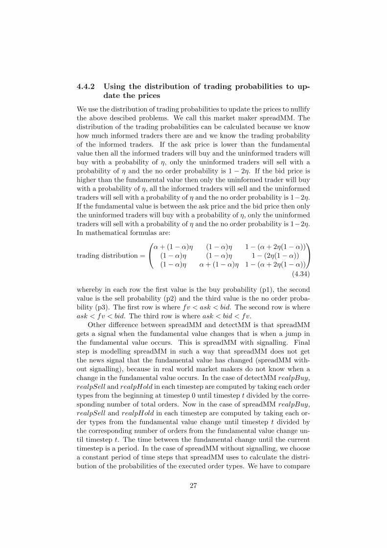
4.4.2 Using the distribution of trading probabilities to up-date the prices

We use the distribution of trading probabilities to update the prices to nullifythe above descibed problems. We call this market maker spreadMM. Thedistribution of the trading probabilities can be calculated because we knowhow much informed traders there are and we know the trading probabilityof the informed traders. If the ask price is lower than the fundamentalvalue then all the informed traders will buy and the uninformed traders willbuy with a probability of η, only the uninformed traders will sell with aprobability of η and the no order probability is 1 − 2η. If the bid price ishigher than the fundamental value then only the uninformed trader will buywith a probability of η, all the informed traders will sell and the uninformedtraders will sell with a probability of η and the no order probability is 1−2η.If the fundamental value is between the ask price and the bid price then onlythe uninformed traders will buy with a probability of η, only the uninformedtraders will sell with a probability of η and the no order probability is 1−2η.In mathematical formulas are:

trading distribution =

α+ (1− α)η (1− α)η 1− (α+ 2η(1− α))(1− α)η (1− α)η 1− (2η(1− α))(1− α)η α+ (1− α)η 1− (α+ 2η(1− α))

(4.34)

whereby in each row the first value is the buy probability (p1), the secondvalue is the sell probability (p2) and the third value is the no order proba-bility (p3). The first row is where fv < ask < bid. The second row is whereask < fv < bid. The third row is where ask < bid < fv.

Other difference between spreadMM and detectMM is that spreadMMgets a signal when the fundamental value changes that is when a jump inthe fundamental value occurs. This is spreadMM with signalling. Finalstep is modelling spreadMM in such a way that spreadMM does not getthe news signal that the fundamental value has changed (spreadMM with-out signalling), because in real world market makers do not know when achange in the fundamental value occurs. In the case of detectMM realpBuy,realpSell and realpHold in each timestep are computed by taking each ordertypes from the beginning at timestep 0 until timestep t divided by the corre-sponding number of total orders. Now in the case of spreadMM realpBuy,realpSell and realpHold in each timestep are computed by taking each or-der types from the fundamental value change until timestep t divided bythe corresponding number of orders from the fundamental value change un-til timestep t. The time between the fundamental change until the currenttimestep is a period. In the case of spreadMM without signalling, we choosea constant period of time steps that spreadMM uses to calculate the distri-bution of the probabilities of the executed order types. We have to compare

27

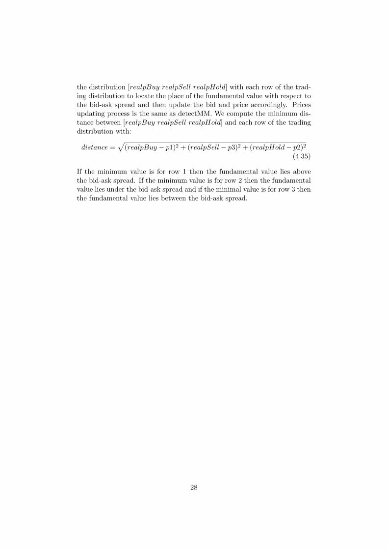
the distribution [realpBuy realpSell realpHold] with each row of the trad-ing distribution to locate the place of the fundamental value with respect tothe bid-ask spread and then update the bid and price accordingly. Pricesupdating process is the same as detectMM. We compute the minimum dis-tance between [realpBuy realpSell realpHold] and each row of the tradingdistribution with:

distance =√

(realpBuy − p1)2 + (realpSell − p3)2 + (realpHold− p2)2

(4.35)

If the minimum value is for row 1 then the fundamental value lies abovethe bid-ask spread. If the minimum value is for row 2 then the fundamentalvalue lies under the bid-ask spread and if the minimal value is for row 3 thenthe fundamental value lies between the bid-ask spread.

28

Chapter 5

Experimental setups

5.1 Fundamental value serie

We have to simulate the value of the fundamental value of the security ineach time during the simulation. We allow changes occur in the fundamen-tal value, because in the real world the fundamental value of the securitycan also change during its lifetime. We generate a sequence of values whichrepresents the fundamental values of the security in each time. We call thesequence the fundamental value serie. The fundamental value serie is gener-ated with the parameters pj, v0, nsteps and sv. Pj is the probability that ajump will occur in the fundamental value. V 0 is the start fundamental value.Nsteps is the number of trades in the simulation. Sv is the standard devia-tion of the jump of the fundamental value. The idea is that in each time t ifa jump takes place with probability pj then the fundamental value at t willbe the fundamental value at time t− 1 plus sv. And if a jump is not takenplace then the fundamental value at time t is the same as the fundamentalvalue at time t− 1. The pseudocode of the function to generate the funda-mental value serie is shown in function fv = GenerateFundamentalValues.jumps is a vector of size nsteps with 0s and 1s. 0 means there is no jumpin the fundamental value and 1 means there is a jump in the fundamen-tal value. Number of jumps is nsteps/pj. Rand is a function to generaterandom numbers between 0 and 1. If the random number is smaller thanpj then the value in the vector is 1 otherwise the value is 0. Jsize is thesize of the jump in de fundamental value and it is calculated by sv times arandom number drawn from a normal distribution. Each fundamental valuein the fundamental value serie is then calculated by v0 plus cumulative sumof (jumps * jsize). An example of such fundamental value serie is shown infigure 5.1. This fundamental value serie is randomly chosen, but we use itbecause the number of jumps in the fundamental value is not too big suchthat the market maker becomes instable and it is not too small such thatwe can see what the market maker does when there are more jumps taking

29

place in a short amount of time.

Function fv = GenerateFundamentalValues(nsteps,sv,pj,v0)

jumps ← [0,rand(nsteps-1) < pj]; jsize ← sv * randn(nsteps);fv ← v0 + cumsum(jumps * jsize);

0 200 400 600 800 10000.98

0.985

0.99

0.995

1

1.005

1.01

1.015

1.02

1.025x 10

4 Fundamental values

Time

Pric

e

Figure 5.1: A fundamental value serie with 1000 time steps.

5.2 Type of trader serie

We have to simulate the arrival of traders for contacting the market markerand trading with them. Our method is generate at random a sequence ofthe numbers 0 to 3 to represent the traders. This sequence of numbers wecall the type of trader serie. For the simulations we need four groups oftraders, which are the informed traders, the uninformed trader who buys,the uninformed trader who sells and the uninformed trader who decidesnot to trade. The total number of traders generated is determined by thenumber of time steps during the simulations. The type of trader serie isgenerated with the parameters α, η and nsteps. Nsteps gives the numberof time steps. α gives the percentage of informed traders. So the number ofinformed traders is calculated by nsteps ∗ α and the number of uninformedtraders is calculated by nsteps ∗ (1 − α). The uninformed traders will be

30

further classified with the parameter η. η is the buy probability or sellprobability of the uninformed trader. The uninformed trader buys or sellswith the same probability η. The uninformed trader holds a trade withprobability 1 − 2 ∗ η. The informed trader we represent with a 0. Theuninformed trader who buys we represent with a 1. The uninformed traderwho sells we represent with a 2. The uninformed trader who does not tradewe represent with a 3. To illustrate this idea we give here an example:nsteps = 12, α = 0.33, η = 0.25 then the type of trader sequence can be

0 1 3 2 1 0 3 3 2 0 0 3

There are 4 informed traders and 8 uninformed traders. 4 of the 8 unin-formed traders hold a trade, 2 buy and 2 sell.

5.3 Market maker’s model parameters estimates

All the three marker maker’s models have the following parameters:

α - this is the fraction of informed traders.

η - this is the probability that an uninformed trader buys or sells.

tt - this is the sequence of type of traders.

pj - this is the probability that a jump will occur.

fvp - this is the fundamental values serie.

buy 0 - this is the start buy price at the beginning of the simulation.

sell 0 - this is the start sell price at the beginning of the simulation.

The Das market maker has these additional parameters:

v0 - this is the initial fundamental value estimate.

sv - this is the standard deviation in the jump of the fundamental value.

SimpleMM has this additional parameter:

γ - this is the convergence rate.

DetectMM and spreadMM have these additional parameters:

∆a - this is the amount of increase or decrease of the ask price.

∆b - this is the amount of increase or decrease of the bid price.

31

In the simulations we let most of the parameters constant. We changeonly a few parameters to analyse the effect of the parameter to the dynamicsof the market maker. The parameters that we change in the simulations isexplained in detail in section 5.6. There are parameters that the marketmaker can control like ∆a and ∆b, because the value of these parameterscan be chosen by the market maker. There are parameters that the marketmaker can’t control for example α and η, because these parameters aredependent of the market situation and the traders in the market.

5.4 The pseudocode of detectMM

The pseudocode of detectMM’s fundamental value location detection isshown in algorithm 1 and the price quoting mechanism is shown in algo-rithm 2. In the code it can be seen that detectMM has to choose three casesaccording to the maximum probabilistic value of Ptrade. This is the portionof buys, sells and no orders from the beginning of the simulation until thetime i. The simulation stops if the stopcondition (number of time steps) ismet. In each case detectMM can choose 3 other decisions according to thetype of order received. In total there are 9 deterministic paths in each timestep for detectMM to choose for. The ask price is then updated with thefunction ask and the bid price is updated with the function bid.

Algorithm 1: Pseudocode of DetectMM’s fundamental value locationdetection algorithm

input : ttoutput: Ptrade, index

ptrade ← ComputePtrade(tt);index ← Max(ptrade);

5.5 The pseudocode of spreadMM

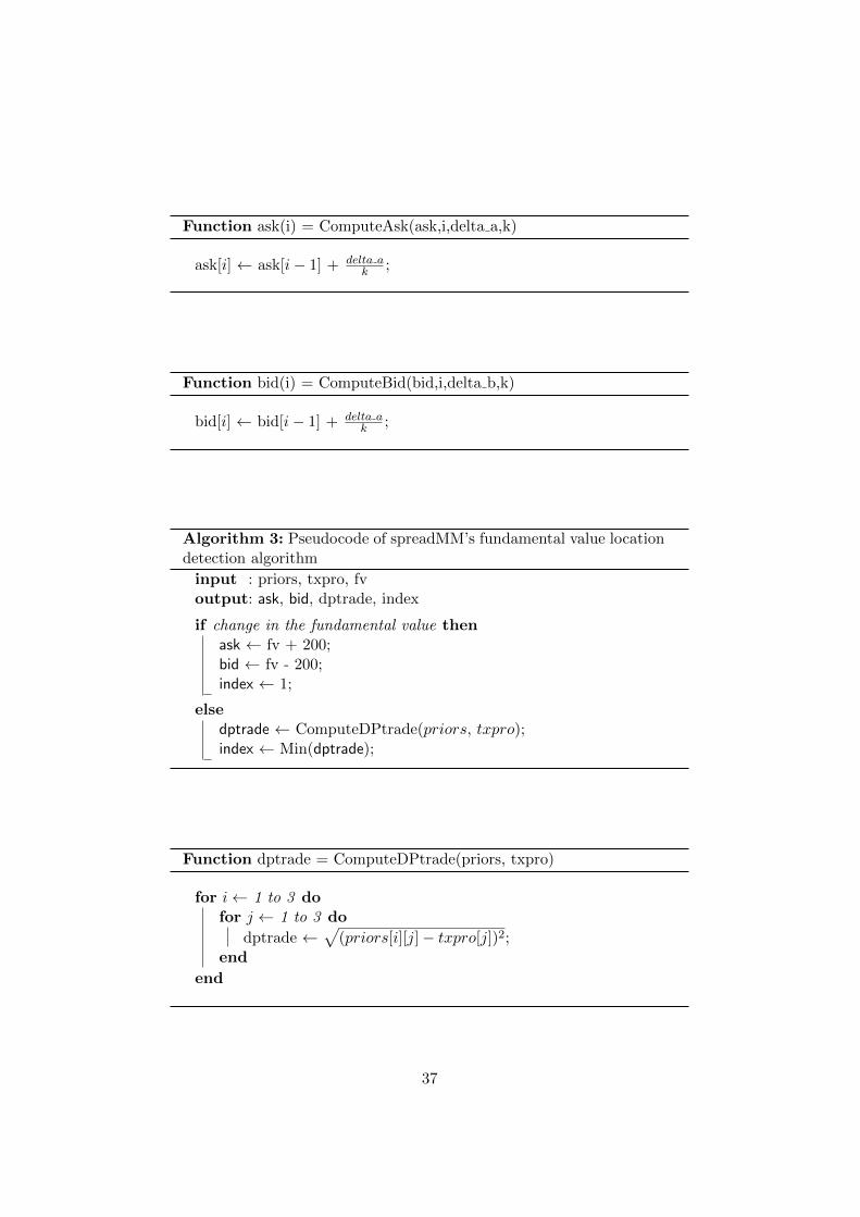
The pseudocode of spreadMM’s fundamental value location detection isshown in algorithm 3 and the price quoting mechanism is shown in algo-rithm 2. In the code it can be seen that spreadMM gets a signal of a changein the fundamental value and sets new ask price to fv + 200 and sets thenew bid price to fv − 200. This is because the market maker receives achange of the fundamental value and does not know what the new bid andask price are and sets a large bid-ask spread. If there is no change in thefundamental value then spreadMM has to choose three cases according tothe minimum value of DPtrade. This is the distance we described in sec-tion 4.4.2 and is computed with equation 4.35. The simulation stops if the

32

stopcondition (number of time steps) is met. In each case spreadMM canchoose 3 other decisions according to the type of order received. In totalthere are 9 deterministic paths in each time step for spreadMM to choosefor. The ask price is then updated with the function ask and the bid priceis updated with the function bid.

5.6 Experimental setup

We use Matlab as the programming environment for programming the code,debugging the code, evaluating the model, and doing simulations. Doingsimulation is the mainly method we use to see the behaviour of the marketmaker. The simulations can be categorized according to these criteria:

1. difference in market maker’s model: Das market maker, simpleMM,detectMM and spreadMM

2. difference in number of simulations: 1 simulation or 100 simulations

3. difference in the values we set for the parameters: α, γ, ∆a, ∆b, k,period

With simpleMM and detectMM we only do single simulations to see theprice dynamics of the market maker mechanism. With single simulation weonly run the simulation 1 time. We use the same fundamental value seriefor the single simulations. We use α’s of 0.25, 0.33, 0.5 and 0.75 to see whatkind of effect the number of informed traders has on the prices quoted bythe two market makers. We set an η of 0.4. For each α we generate thecorresponding trader type serie, because the trader type serie depends onthe α chosen. This parameter tells the probability of an uninformed traderto buy or sell. If η is 0.4 then the buy probability is 0.4 and also the sellprobability is 0.4 and the no order probability is of course 0.2.

To simulate spreadMM we do 100 simulations. And we calculate in eachtime step the mean bid price and ask price over the 100 simulations. Forexample at t = 1 the mean bid price over the 100 simulations is calculatedas follows: Adding the bid price in each simulation of t = 1. We do thiswith all the bid prices in time steps from t = 1 to t = 1000. After thiswe get 1000 mean bid prices. Likewise, we do the same with the ask price.We plot the mean bid price curve and the mean ask price curve with thefundamental value curve in the same figure. To see what spreadMM willdo in situation where the fundamental value is stable for a long time, wegenerate a fundamental value with only one jump during the simulation.The first 500 time steps the fundamental value is 10000 and last 500 timesteps the fundamental steps is 10020. We create this fundamental value withonly one change in the fundamental value in the middle of the simulationtime and change the parameters to get an insight of what kind of effect have

33

on the parameters to the bid and ask prices and if the market maker usingdistribution of orders from the order flow can track the fundamental value.We generate 100 type of trader series each with an α of 0.25 and then also thesame with an α of 0.33, 0.5, 0.75. The experiments can be categorized intothree groups. In the first group of experiments the change in the experimentis the parameter α. There are four experiments in this group. We set η to0.4, ∆a and ∆b to 40 and k = 1, 2, 3, ... and if the first derivative of theprice in time t = 0 we set k back to 0 or else we increase k with 1 in thenext time step. The goal of this group of experiments is to see what kind ofeffect the population of informed traders has on the price setting behaviourof the market maker. In the second group of experiments we set α to 0.75and η to 0.4 and we do with the parameter k the same as in the first groupof experiments, but we set ∆a and ∆b in the simulations to the values of10, 30, 50, 70, 90 or 200. In the third group of experiments we set α to 0.75and η to 0.4, ∆a and ∆b to 90 and we change k in the experiments to 1,2, 4, or 6, but now in each time step the value of k is fixed and does notchange during the simulation as the first group of experiments does. We dothe simulations of spreadMM with signalling and without signalling. In caseof spreadMM without signalling, we do simulations with constant periods of5, 10, 20, 25, 30 and 60.

We simulate the Das market maker with α’s of 0.25, 0.33, 0.5 and 0.75and an η of 0.4. We compare the result of the simulation of the Das marketmaker with the result of the simulation of spreadMM.

5.7 Model evaluation and Performance measure

5.7.1 Model evaluation of detectMM and spreadMM

For evaluation and benchmarking the market maker’s model we use twomethods. The first method is the mean of bid-ask spreads method. Thesecond method is sum of difference between the fundamental value and theprices as performance measure.

5.7.2 Mean bid-ask spreads

To average the 100 simulations we use for comparison the mean of bid-askspreads as performance measure. After the 100 simulations we computethe mean of bid-ask spreads of the 100 simulations. The mean of bid-askspreads is calculated by adding the bid-ask spread in each timestep togetherand divide by the number of timesteps in the simulation. In mathematicalformula this will be:

mean of bid-ask spreads =

∑at − bt

Number of timesteps(5.1)

34

Sum of diffence between the fundamental value and the prices

For benchmarking the performance of the Das market maker and spreadMMwe compute the sum of difference between the fundamental value and the bidprice (sumdifbid), the sum of the difference between the fundamental valueand the ask price (sumdifask) and the average of the two (avaragesumdif).In mathematical formulas:

sumdifbid =∑

(fvt − bidt) (5.2)

sumdifask =∑

(askt − fvt) (5.3)

averagesumdif =(sumdifbid+ sumdifask)

2(5.4)

35

Algorithm 2: Pseudocode of DetectMM and SpreadMM price quotingalgorithm

input : index, order, delta a, delta b,koutput: ask [i], bid [i]

for i← 1 to n doswitch index do

case index is 1if order is 1 then

ask [i] ← ComputeAsk(ask,i,delta a,k);bid [i] ← bid [i− 1];

else if order is -1 thenask [i] ← ask [i− 1];bid [i] ← ComputeBid(bid,i,delta b,k);

else order is 0ask [i] ← ComputeAsk(ask,i,delta a,k);bid [i] ← ComputeBid(ask,i,delta b,k);

case index is 2if order is 1 then

ask [i] ← ComputeAsk(ask,i,-delta a,k);bid [i] ← bid [i− 1];if ask [i] < bid [i] then ask [i] = bid [i];

else if order is -1 thenask [i] ← ask [i− 1];bid [i] ← ComputeBid(bid,i,-delta b,k);if bid [i] < ask [i] then bid [i] > ask [i];

else order is 0ask [i] ← ComputeAsk(ask,i,-delta a,k);bid [i] ← ComputeBid(ask,i,-delta b,k);

case index is 3if order is 1 then

ask [i] ← ComputeAsk(ask,i,-delta a,k);bid [i] ← bid [i− 1];if ask [i] < bid [i] then ask [i] = bid [i];

else if order is -1 thenask [i] ← ask [i− 1];bid [i] ← ComputeBid(bid,i,delta b,k);if bid [i] < ask [i] then bid [i] > ask [i];

else order is 0ask [i] ← ComputeAsk(ask,i,-delta a,k);bid [i] ← ComputeBid(ask,i,delta b,k);

36

Function ask(i) = ComputeAsk(ask,i,delta a,k)

ask[i] ← ask[i− 1] + delta ak ;

Function bid(i) = ComputeBid(bid,i,delta b,k)

bid[i] ← bid[i− 1] + delta ak ;

Algorithm 3: Pseudocode of spreadMM’s fundamental value locationdetection algorithm

input : priors, txpro, fvoutput: ask, bid, dptrade, index

if change in the fundamental value thenask ← fv + 200;bid ← fv - 200;index ← 1;

elsedptrade ← ComputeDPtrade(priors, txpro);index ← Min(dptrade);

Function dptrade = ComputeDPtrade(priors, txpro)

for i← 1 to 3 dofor j ← 1 to 3 do

dptrade ←√

(priors[i][j]− txpro[j])2;end

end

37

Chapter 6

Results

In this chapter we describe the results of the experiments we have simulatedwith the Das market maker (see chapter 3) and with the market makerssimpleMM (see chapter 4.3) , detectMM (see chapter 4.4.1) and spreadMM(see chapter 4.4.2).

6.1 Simulation results of single experiments

6.1.1 Experiment with simpleMM

0 200 400 600 800 10000.98

0.985

0.99

0.995

1

1.005

1.01

1.015

1.02

1.025x 10

4

Time

Pric

e

SimpleMM

bidaskfv

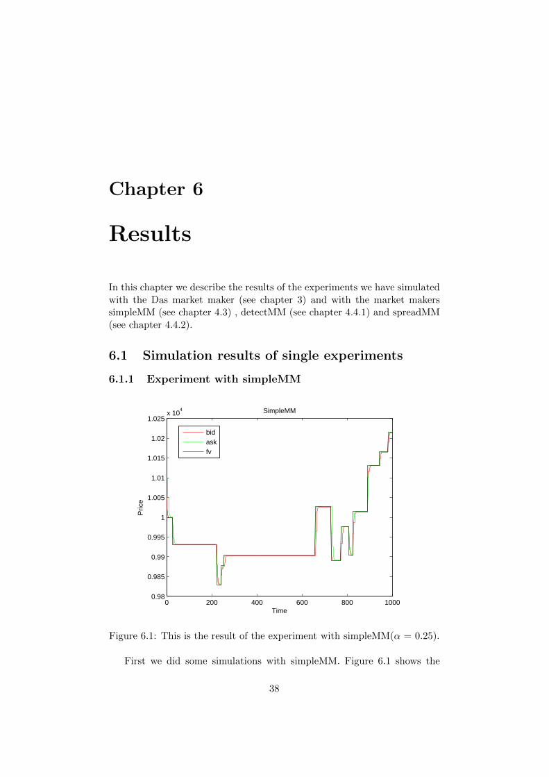
Figure 6.1: This is the result of the experiment with simpleMM(α = 0.25).

First we did some simulations with simpleMM. Figure 6.1 shows the

38

bid price, the ask price and the fundamental value of the simulations withsimpleMM. We only show the figure of the result of the experiment with anα of 0.25 here. The results of the simulations with α’s of 0.33, 0.5 and 0.75 isshown in appendix A, because the figures are mostly identical to each other.SimpleMM can track the fundamental value, because the market maker isassumed to know the fundamental value. After a jump in the fundamentalvalue it can be clearly seen that there occurs a little delay in time before themarket maker gets to the correct fundamental value. How fast the pricesconverge to the fundamental value is determined by the parameter γ. If γ isnearer to 0 then the prices will slower converge. If γ is nearer to 1 then theprices will converge faster. The bid price and the ask price in the same timestep in the simulations are not the same, due to different trader type serieswe have used and so the order flow in the four simulation is also different.

6.1.2 Experiments with detectMM

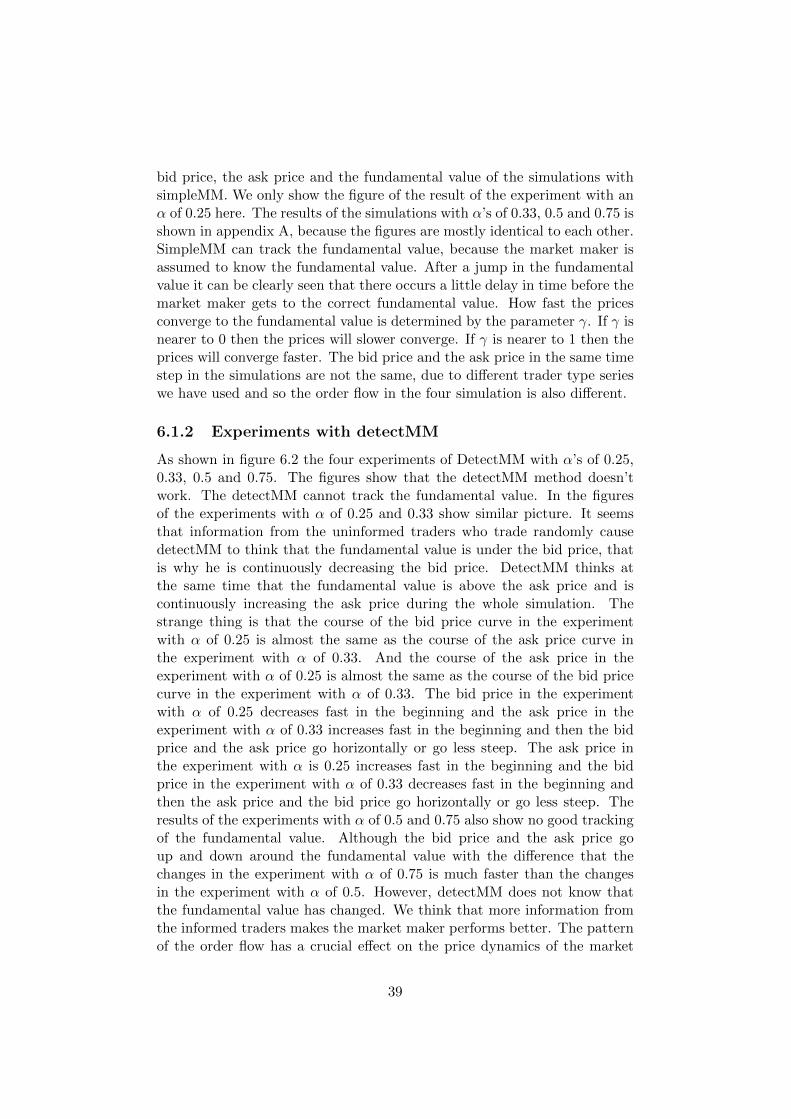
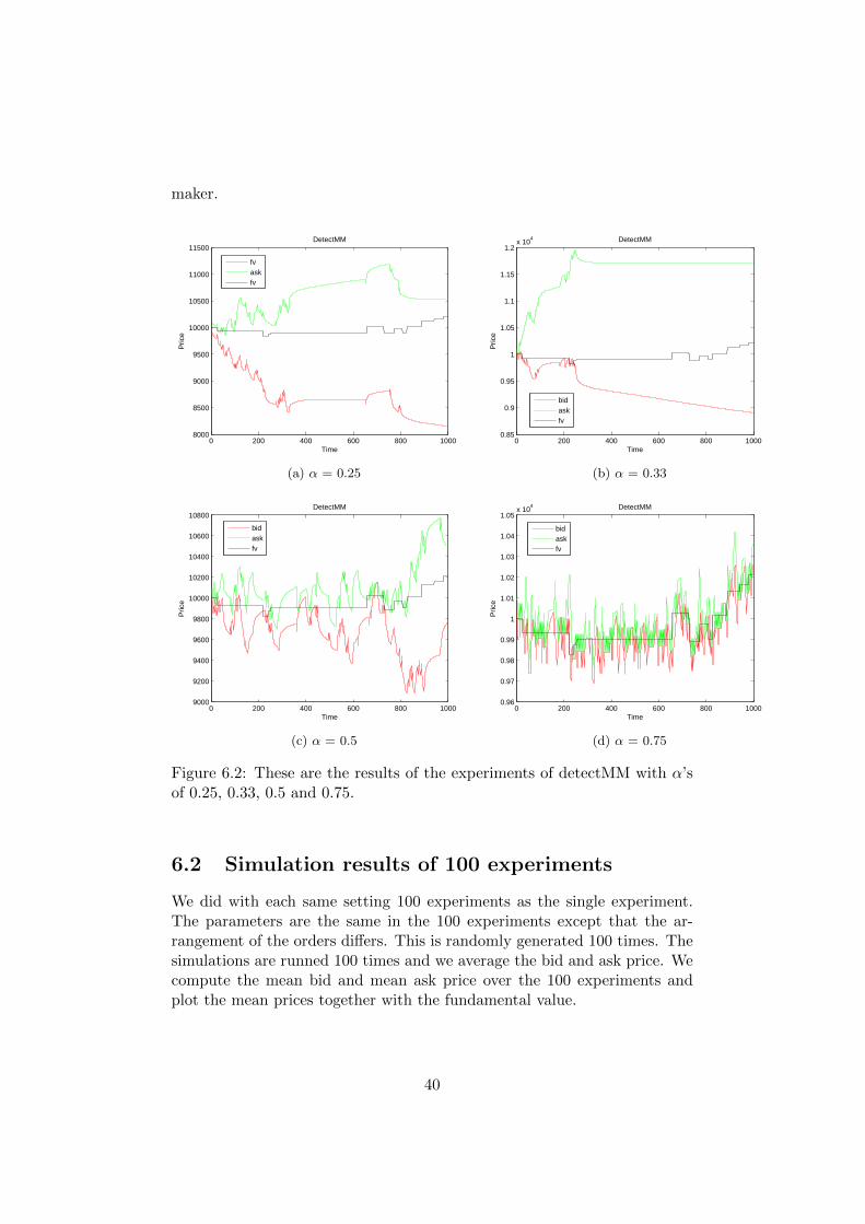
As shown in figure 6.2 the four experiments of DetectMM with α’s of 0.25,0.33, 0.5 and 0.75. The figures show that the detectMM method doesn’twork. The detectMM cannot track the fundamental value. In the figuresof the experiments with α of 0.25 and 0.33 show similar picture. It seemsthat information from the uninformed traders who trade randomly causedetectMM to think that the fundamental value is under the bid price, thatis why he is continuously decreasing the bid price. DetectMM thinks atthe same time that the fundamental value is above the ask price and iscontinuously increasing the ask price during the whole simulation. Thestrange thing is that the course of the bid price curve in the experimentwith α of 0.25 is almost the same as the course of the ask price curve inthe experiment with α of 0.33. And the course of the ask price in theexperiment with α of 0.25 is almost the same as the course of the bid pricecurve in the experiment with α of 0.33. The bid price in the experimentwith α of 0.25 decreases fast in the beginning and the ask price in theexperiment with α of 0.33 increases fast in the beginning and then the bidprice and the ask price go horizontally or go less steep. The ask price inthe experiment with α is 0.25 increases fast in the beginning and the bidprice in the experiment with α of 0.33 decreases fast in the beginning andthen the ask price and the bid price go horizontally or go less steep. Theresults of the experiments with α of 0.5 and 0.75 also show no good trackingof the fundamental value. Although the bid price and the ask price goup and down around the fundamental value with the difference that thechanges in the experiment with α of 0.75 is much faster than the changesin the experiment with α of 0.5. However, detectMM does not know thatthe fundamental value has changed. We think that more information fromthe informed traders makes the market maker performs better. The patternof the order flow has a crucial effect on the price dynamics of the market

39

maker.

0 200 400 600 800 10008000

8500

9000

9500

10000

10500

11000

11500

Time

Pric

e

DetectMM

fvaskfv

(a) α = 0.25

0 200 400 600 800 10000.85

0.9

0.95

1

1.05

1.1

1.15

1.2x 10

4

Time

Pric

e

DetectMM

bidaskfv

(b) α = 0.33

0 200 400 600 800 10009000

9200

9400

9600

9800

10000

10200

10400

10600

10800

Time

Pric

e

DetectMM

bidaskfv

(c) α = 0.5

0 200 400 600 800 10000.96

0.97

0.98

0.99

1

1.01

1.02

1.03

1.04

1.05x 10

4

Time

Pric

e

DetectMM

bidaskfv

(d) α = 0.75

Figure 6.2: These are the results of the experiments of detectMM with α’sof 0.25, 0.33, 0.5 and 0.75.

6.2 Simulation results of 100 experiments

We did with each same setting 100 experiments as the single experiment.The parameters are the same in the 100 experiments except that the ar-rangement of the orders differs. This is randomly generated 100 times. Thesimulations are runned 100 times and we average the bid and ask price. Wecompute the mean bid and mean ask price over the 100 experiments andplot the mean prices together with the fundamental value.

40

6.2.1 Simulation with SpreadMM

Fundamental value serie with 1 jump

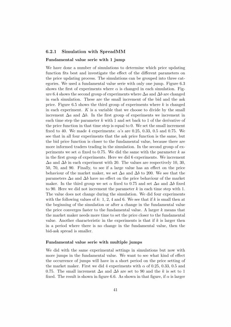
We have done a number of simulations to determine which price updatingfunction fits best and investigate the effect of the different parameters onthe price updating process. The simulations can be grouped into three cat-egories. We used a fundamental value serie with only one jump. Figure 6.3shows the first of experiments where α is changed in each simulation. Fig-ure 6.4 shows the second group of experiments where ∆a and ∆b are changedin each simulation. These are the small increment of the bid and the askprice. Figure 6.5 shows the third group of experiments where k is changedin each experiment. K is a variable that we choose to divide by the smallincrement ∆a and ∆b. In the first group of experiments we increment ineach time step the parameter k with 1 and set back to 1 of the derivative ofthe price function in that time step is equal to 0. We set the small incrementfixed to 40. We made 4 experiments: α’s are 0.25, 0.33, 0.5 and 0.75. Wesee that in all four experiments that the ask price function is the same, butthe bid price function is closer to the fundamental value, because there aremore informed traders trading in the simulation. In the second group of ex-periments we set α fixed to 0.75. We did the same with the parameter k asin the first group of experiments. Here we did 6 experiments. We increment∆a and ∆b in each experiment with 20. The values are respectively 10, 30,50, 70, and 90. Finally, to see if a large value has an effect on the pricebehaviour of the market maker, we set ∆a and ∆b to 200. We see that theparameters ∆a and ∆b have no effect on the price behaviour of the marketmaker. In the third group we set α fixed to 0.75 and set ∆a and ∆b fixedto 90. Here we did not increment the parameter k in each time step with 1.The value does not change during the simulation. We did four experimentswith the following values of k: 1, 2, 4 and 6. We see that if k is small then atthe beginning of the simulation or after a change in the fundamental valuethe price converges faster to the fundamental value. A larger k means thatthe market maker needs more time to set the price closer to the fundamentalvalue. Another characteristic in the experiments is that if k is larger thenin a period where there is no change in the fundamental value, then thebid-ask spread is smaller.

Fundamental value serie with multiple jumps

We did with the same experimental settings in simulations but now withmore jumps in the fundamental value. We want to see what kind of effectthe occurrence of jumps will have in a short period on the price setting ofthe market maker. First we did 4 experiments with α of 0.25, 0.33, 0.5 and0.75. The small increment ∆a and ∆b are set to 90 and the k is set to 1fixed. The result is shown in figure 6.6. As shown in that figure, if α is larger

41

0 200 400 600 800 10000.996

0.998

1

1.002

1.004

1.006

1.008

1.01

1.012x 10

4

Time

Pric

e

SpreadMM

bidaskfv

(a) α = 0.25

0 200 400 600 800 10000.998

1

1.002

1.004

1.006

1.008

1.01

1.012x 10

4

Time

Pric

e

SpreadMM

bidaskfv

(b) α = 0.33

0 200 400 600 800 10000.998

1

1.002

1.004

1.006

1.008

1.01

1.012x 10

4

Time

Pric

e

SpreadMM

bidaskfv

(c) α = 0.5

0 200 400 600 800 10000.998

1

1.002

1.004

1.006

1.008

1.01

1.012x 10

4

Time

Pric

e

SpreadMM

bidaskfv

(d) α = 0.75

Figure 6.3: These are the results of the experiments of spreadMM withsignalling and α’s of 0.25, 0.33, 0.5 and 0.75.

42

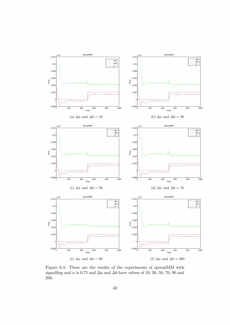
0 200 400 600 800 10000.998

1

1.002

1.004

1.006

1.008

1.01

1.012x 10

4

Time

Pric

e

SpreadMM

bidaskfv

(a) ∆a and ∆b = 10

0 200 400 600 800 10000.998

1

1.002

1.004

1.006

1.008

1.01

1.012x 10

4

Time

Pric

e

SpreadMM

bidaskfv

(b) ∆a and ∆b = 30

0 200 400 600 800 10000.998

1

1.002

1.004

1.006

1.008

1.01

1.012x 10

4

Time

Pric

e

SpreadMM

bidaskfv

(c) ∆a and ∆b = 50

0 200 400 600 800 10000.998

1

1.002

1.004

1.006

1.008

1.01

1.012x 10

4

Time

Pric

e

SpreadMM

bidaskfv

(d) ∆a and ∆b = 70

0 200 400 600 800 10000.998

1

1.002

1.004

1.006

1.008

1.01

1.012x 10

4

Time

Pric

e

SpreadMM

bidaskfv

(e) ∆a and ∆b = 90

0 200 400 600 800 10000.998

1

1.002

1.004

1.006

1.008

1.01

1.012x 10

4

Time

Pric

e

SpreadMM

bidaskfv

(f) ∆a and ∆b = 200

Figure 6.4: These are the results of the experiments of spreadMM withsignalling and α is 0.75 and ∆a and ∆b have values of 10, 30, 50, 70, 90 and200.

43

0 200 400 600 800 10000.996

0.998

1

1.002

1.004

1.006

1.008

1.01

1.012x 10

4

Time

Pric

e

SpreadMM

bidaskfv

(a) k = 1

0 200 400 600 800 10000.996

0.998

1

1.002

1.004

1.006

1.008

1.01

1.012x 10

4

Time

Pric

e

SpreadMM

bidaskfv

(b) k = 2

0 200 400 600 800 10000.994

0.996

0.998

1

1.002

1.004

1.006

1.008

1.01

1.012x 10

4

Time

Pric

e

SpreadMM

bidaskfv

(c) k = 4

0 200 400 600 800 10000.994

0.996

0.998

1

1.002

1.004

1.006

1.008

1.01

1.012x 10

4

Time

Pric

e

SpreadMM

bidaskfv

(d) k = 6

Figure 6.5: These are the results of the experiments of spreadMM withsignalling and α is 0.75 and ∆a and ∆b are 90 and k is 1, 2, 4 or 6.

44

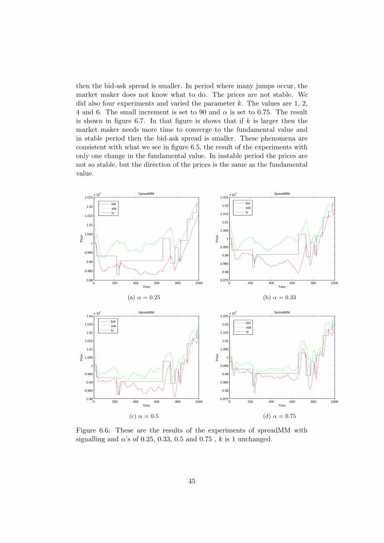
then the bid-ask spread is smaller. In period where many jumps occur, themarket maker does not know what to do. The prices are not stable. Wedid also four experiments and varied the parameter k. The values are 1, 2,4 and 6. The small increment is set to 90 and α is set to 0.75. The resultis shown in figure 6.7. In that figure is shows that if k is larger then themarket maker needs more time to converge to the fundamental value andin stable period then the bid-ask spread is smaller. These phenomena areconsistent with what we see in figure 6.5, the result of the experiments withonly one change in the fundamental value. In instable period the prices arenot so stable, but the direction of the prices is the same as the fundamentalvalue.

0 200 400 600 800 10000.98

0.985

0.99

0.995

1

1.005

1.01

1.015

1.02

1.025x 10

4

Time

Pric

e

SpreadMM

bidaskfv

(a) α = 0.25

0 200 400 600 800 10000.975

0.98

0.985

0.99

0.995

1

1.005

1.01

1.015

1.02

1.025x 10

4

Time

Pric

e

SpreadMM

bidaskfv

(b) α = 0.33

0 200 400 600 800 10000.98

0.985

0.99

0.995

1

1.005

1.01

1.015

1.02

1.025

1.03x 10

4

Time

Pric

e

SpreadMM

bidaskfv

(c) α = 0.5

0 200 400 600 800 10000.975

0.98

0.985

0.99

0.995

1

1.005

1.01

1.015

1.02

1.025x 10

4

Time

Pric

e

SpreadMM

bidaskfv

(d) α = 0.75

Figure 6.6: These are the results of the experiments of spreadMM withsignalling and α’s of 0.25, 0.33, 0.5 and 0.75 , k is 1 unchanged.

45

0 200 400 600 800 10000.975

0.98

0.985

0.99

0.995

1

1.005

1.01

1.015

1.02

1.025x 10

4

Time

Pric

e

SpreadMM

bidaskfv

(a) k = 1

0 200 400 600 800 10000.98

0.985

0.99

0.995

1

1.005

1.01

1.015

1.02

1.025x 10

4

Time

Pric

e

SpreadMM

bidaskfv

(b) k = 2

0 200 400 600 800 10000.98

0.985

0.99

0.995

1

1.005

1.01

1.015

1.02

1.025x 10

4

Time

Pric

e

SpreadMM

bidaskfv

(c) k = 4

0 200 400 600 800 10000.98

0.985

0.99

0.995

1

1.005

1.01

1.015

1.02

1.025x 10

4

Time

Pric

e

SpreadMM

askbidfv

(d) k = 6

Figure 6.7: These are the results of the experiments of spreadMM withsignalling and α is 0.75 and ∆a and ∆b are 90 and k is 1, 2, 4 or 6.

46

SpreadMM and fundamental value approximation

In the above experiments with spreadMM, the market maker gets the newssignal that the fundamental value is changed and from that time step on tothe current time step the distribution of the probability of buy, sell and noorder is calculated. These calculated probabilities are then compared withthe distribution of the prior probability of buy, sell and no order using thedistance method (see equation 4.35). However, we want to model in a waysuch that the market maker does not know whether a fundamental changehas taken place or not. The results of the experiments with fundamentalvalue approximation are shown in figure 6.8. We did 6 experiments. Eachsimulation we varied the size of the period wherein the market maker calcu-lates the probabilities. The total number of orders in equations 4.8, 4.9 and4.10 in each time step of this period is equal to current timestep minus thenumber of timesteps since the beginning of the chosen size of the period. Asit is seen in the results if the chosen period is large then the market makerwill become more uncertain and lead to a large bid-ask spread and unstableprices.

6.2.2 Simulation with the Das market maker

We did experiments with the Das market maker with α is 0.75 and η is0.4. The result is shown in figure 6.9. The figure shows that after eachjump in the fundamental value the market maker sets a very large bid-askspread. He gets a signal if a change in the fundamental value has takenplaced. After a jump the market maker needs time to converge to the newfundamental value. Unlike spreadMM, the Das market maker is in unstableperiod where there occur more than one jump also very stable and can trackthe fundamental value.

6.3 Comparison between Das market maker andSpreadMM

6.3.1 Using the mean of bid-ask spreads method

We use mean of bid-ask spreads method to compare the performance be-tween the Das market maker and spreadMM. We summarise the bid-askspreads of each time step and divide it by the number of time step. Smallbid-ask spreads are preferred by the market maker. So if the mean sum ofbid-ask spreads is small, then this means that the market maker is doing agood job. Figure 6.10 shows 4 experiments with the following market makersand settings (from above to below and from left to right):

• Das market maker

47

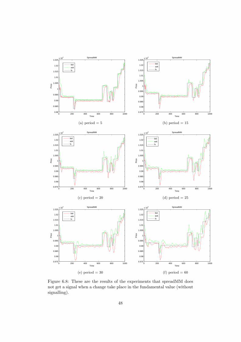
0 200 400 600 800 10000.98

0.985

0.99

0.995

1

1.005

1.01

1.015

1.02

1.025x 10

4

Time

Pric

e

SpreadMM

bidaskfv

(a) period = 5

0 200 400 600 800 10000.975

0.98

0.985

0.99

0.995

1

1.005

1.01

1.015

1.02

1.025x 10

4

Time

Pric

e

SpreadMM

bidaskfv

(b) period = 15

0 200 400 600 800 10000.975

0.98

0.985

0.99

0.995

1

1.005

1.01

1.015

1.02

1.025x 10

4

Time

Pric

e

SpreadMM

bidaskfv

(c) period = 20

0 200 400 600 800 10000.975

0.98

0.985

0.99

0.995

1

1.005

1.01

1.015

1.02

1.025x 10

4

Time

Pric

e

SpreadMM

bidaskfv

(d) period = 25

0 200 400 600 800 10000.975

0.98

0.985

0.99

0.995

1

1.005

1.01

1.015

1.02

1.025x 10

4

Time

Pric

e

SpreadMM

bidaskfv

(e) period = 30

0 200 400 600 800 10000.975

0.98

0.985

0.99

0.995

1

1.005

1.01

1.015

1.02

1.025x 10

4

Time

Pric

e

SpreadMM

bidaskfv

(f) period = 60

Figure 6.8: These are the results of the experiments that spreadMM doesnot get a signal when a change take place in the fundamental value (withoutsignalling).

48

0 200 400 600 800 10000.98

0.985

0.99

0.995

1

1.005

1.01

1.015

1.02

1.025

1.03x 10

4

Time

Pric

e

Das

bidaskfv

Figure 6.9: This is the result of the experiment with the Das market maker(α = 0.75).

• SpreadMM with fundamental value changing signalling (k is 6 and isfixed in each time step)

• SpreadMM with fundamental value changing signalling (k is incre-mented in time step)

• SpreadMM without fundamental value changing signalling (period is10)

Each figure plots the probabilistic density function of the mean of bid-askspreads over the 100 simulations generated by the market maker. The Dasmarket maker has generated mean of bid-ask spreads between 14 and 22.SpreadMM with fundamental value changing signalling and fixed k has gen-erated mean of bid-ask spreads between 68 and 90. SpreadMM with funda-mental value changing signalling and k is incremented has generated meanof bid-ask spreads between 20 and 110. The spreadMM without fundamen-tal value changing signalling has generated mean of bid-ask spreads between16 and 36. We also put the result of the experiments of spreadMM with-out signalling, but varied the size of the period wherein the market makercalculates the probabilities to adjust the prices in figure 6.11. As shown infigure 6.11 if the period is large, for example 30 and 60, then the mean ofbid-ask spreads is also increasing.

49

13 14 15 16 17 18 19 20 21 22 230

0.05

0.1

0.15

0.2

0.25

0.3

0.35Das

Mean of Bid−Ask Spreads

Pro

babi

litie

s

(a) Das market maker

65 70 75 80 85 90 950

0.02

0.04

0.06

0.08

0.1

0.12

0.14

0.16

0.18

Mean of Bid−Ask Spreads

Pro

babi

litie

s

(b) SpreadMM with signalling (k is fixed)

10 20 30 40 50 60 70 80 90 100 1100

0.005

0.01

0.015

0.02

0.025

0.03

Mean of Bid−Ask Spreads

Pro

babi

litie

s

(c) SpreadMM with signalling (k is incremented

16 18 20 22 24 26 28 30 32 34 360

0.02

0.04

0.06

0.08

0.1

0.12

0.14

0.16

Mean of Bid−Ask Spreads

SpreadMM

Pro

babi

litie

s

(d) SpreadMM without signalling

Figure 6.10: These are the results of the probabilistic density function ofthe mean of bid-ask spreads (with α is 0.75).

50

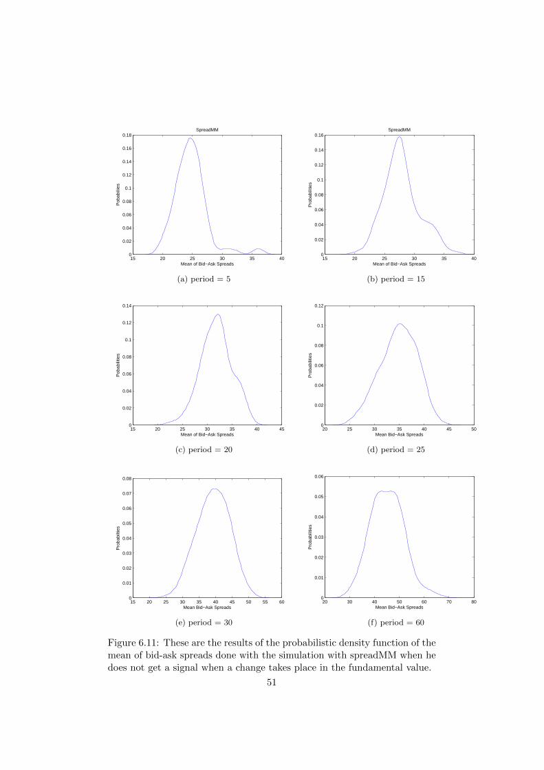
15 20 25 30 35 400

0.02

0.04

0.06

0.08

0.1

0.12

0.14

0.16

0.18

Mean of Bid−Ask Spreads

SpreadMM

Pob

abili

ies

(a) period = 5

15 20 25 30 35 400

0.02

0.04

0.06

0.08

0.1

0.12

0.14

0.16

Mean of Bid−Ask Spreads

Pro

babi

litie

s

SpreadMM

(b) period = 15

15 20 25 30 35 40 450

0.02

0.04

0.06

0.08

0.1

0.12

0.14

Mean of Bid−Ask Spreads

Pob

abili

ties

(c) period = 20

20 25 30 35 40 45 500

0.02

0.04

0.06

0.08

0.1

0.12

Mean Bid−Ask Spreads

Pro

babi

litie

s

(d) period = 25

15 20 25 30 35 40 45 50 55 600

0.01

0.02

0.03

0.04

0.05

0.06

0.07

0.08

Mean Bid−Ask Spreads

Pro

babi

lties

(e) period = 30

20 30 40 50 60 70 800

0.01

0.02

0.03

0.04

0.05

0.06

Mean Bid−Ask Spreads

Pro

babi

litie

s

(f) period = 60

Figure 6.11: These are the results of the probabilistic density function of themean of bid-ask spreads done with the simulation with spreadMM when hedoes not get a signal when a change takes place in the fundamental value.

51

6.3.2 Using the sum of difference between the fundamentalvalue and the price method

We use the sum of difference between the fundamental value and the pricesmethod to compare the performance of Das market maker and the diversesettings of spreadMM, because the mean of bid-ask spreads method saysnothing about how close the market maker is tracking the real fundamentalvalue. We use the same models described in 6.3.1 about the mean of bid-askspreads method for camparisons. Table 6.1 and table 6.2 list the sum ofdifference between fundamental value and bid price, the sum of differencebetween fundamental value and ask price and the mean of the models. Thetables show that the Das market maker tracks the fundamental value betterthan spreadMM. SpreadMM with signalling where k is incremented has alarger difference than spreadMM with signalling where k is fixed. As welook at the results of spreadMM without signalling then we can see thatthe larger the period that spreadMM uses to calculate the probabilities thelarger the difference is.

Table 6.1: Table sum of difference between fv and prices 1

Model diffbid diffask diffmean

Das market maker 9173.01 8772.91 8972.96SpreadMM with signalling (k is fixed) 32081.67 36807.07 34444.60

SpreadMM with signalling(k is incremented) 53611.97 47586.65 50599.31SpreadMM without signalling (period is 10) 20551.46 17329.24 18940.35

Table 6.2: Table sum of difference between fv and prices 2

Model diffbid diffask diffmean

SpreadMM without signalling (period is 5) 19345.90 16909.15 18127.53SpreadMM without signalling (period is 15) 21250.09 19432.14 20341.12SpreadMM without signalling (period is 20) 23063.50 20625.36 21844.43SpreadMM without signalling (period is 25) 26505.41 23727.31 25116.36SpreadMM without signalling (period is 30) 28929.41 26512.80 27721.10SpreadMM without signalling (period is 60) 32939.29 32425.62 32682.46

52

6.4 Conclusion

SimpleMM can quote prices which reflect the true fundamental value, be-cause it is assumed that he knows the fundamental value. DetectMM doesnot work, because of the shortcomings of the model. If we compare theDas market maker with spreadMM both with the mean of bid-ask spreadsmethod and the sum difference between the fundamental value and the bidand ask price then we see that the Das market maker performs better, be-cause the Das market maker keeps a probability distribution of all possiblefundamental values. Das market maker has more information to approx-imate the fundamental value than spreadMM. SpreadMM can track thefundamental value, but it is not perfect. Advantage of spreadMM over theDas market maker is that spreadMM uses a simpler fundamental value ap-proximation method so that spreadMM uses less computation time.

53

Chapter 7

Conclusion and futureresearch

7.1 Conclusion

Market makers play a very important role in today’s financial markets. Oneof the main task of the market maker is to execute investors’ orders at thebest possible price. How does the market maker know what is the bestprice to create liquidity and at the same time profits from the trade? Howdoes a market maker quote the bid and ask prices? Using a model we canstudy the pricing mechanism of the market maker. Market makers are usinginside knowledge, experience to set prices on a daily basis. The order flowis one of the information a market maker uses. The question is whether theorder flow contains information for the market maker to track the underlyingfundamental value. In this thesis we have conducted a research on marketmarker’s models. We introduced a simple linear market maker’s price settingfunction with the fundamental value in it. This is not consistent with the realworld. Then we introduced the method of using the order flow informationto locate the position of the fundamental value with respect to the bid-askspread. We first use the maximum value of probability order type in theorder flow to determine the position of the fundamental value. However,because of the drawbacks of this method we introduced another methodto use. Then we used the distribution of the probability of the order typein the order flow to determine the fundamental value. And the marketmaker gets a signal if the fundamental value changes. In the real worldthe market maker does not know in advance that the fundamental value isgoing to change. That’s why the market maker calculates the probabilitiesnot since a change occurs in the fundamental value, but from each smallperiods of time the market maker begins to compute the probabilities. Wecompared this market maker with the Das market maker using the mean ofbid-ask spreads method and the difference between the fundamental value

54

and the prices method. We conclude that the information in order flow doesindeed contain information that the market maker can use to update theprices, but this only works in certain situations. For example if the period isrelatively small then the information is more useful. Using the mean of bid-ask spreads method to compare the performance of the Das market makerand the in this paper introduced market maker spreadMM shows that theDas market maker is better, because he generates smaller bid-ask spreads.If we compare the mean of bid-ask spreads that is generated by spreadMMbut with varied size of periods that the market maker is using to calculatesthe probabilities to adjust the prices then the results show that the largerthe period the larger the bid-ask spread. If we compare the models withthe sum difference between the fundamental value and the prices we also seethat the Das market maker performs better than spreadMM.

7.2 Future research

These are the possible recommendations we suggest to conduct further re-search:

• We suggest to use probabilistic fuzzy system to model the probabilitydensity of the order types in the order flow. It is good to model theorder flow process as a probabilistic fuzzy system, because the proba-bilistic uncertainty of the orders placed by investors can be modelledand better understanding of the order flow process can be gained.

• The smallest increments ∆a and ∆b in the price updating functionare fixed in each time step. We suggest to change this amount ofincrementation in each time step, because the distance between theprices and the fundamental value differs in each time step, so theincrementation should also be different in each time step to updatethe prices.

55

Appendix A

Figures

0 200 400 600 800 10000.98

0.985

0.99

0.995

1

1.005

1.01

1.015

1.02

1.025x 10

4

Time

Pric

e

SimpleMM

bidaskfv

(a) α = 0.33

0 200 400 600 800 10000.98

0.985

0.99

0.995

1

1.005

1.01

1.015

1.02

1.025x 10

4

Time

Pric

e

SimpleMM

bidaskfv

(b) α = 0.5

0 200 400 600 800 10000.98

0.985

0.99

0.995

1

1.005

1.01

1.015

1.02

1.025x 10

4

Time

Pric

e

SimpleMM

bidaskfv

(c) α = 0.75

Figure A.1: These are the results of the experiments with simpleMM.

56

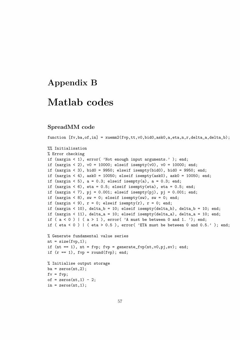
Appendix B

Matlab codes

SpreadMM code

function [fv,ba,of,in] = xuemm2(fvp,tt,v0,bid0,ask0,a,eta,n,r,delta_a,delta_b);

%% Initialisation

% Error checking

if (nargin < 1), error( ’Not enough input arguments.’ ); end;

if (nargin < 2), v0 = 10000; elseif isempty(v0), v0 = 10000; end;

if (nargin < 3), bid0 = 9950; elseif isempty(bid0), bid0 = 9950; end;

if (nargin < 4), ask0 = 10050; elseif isempty(ask0), ask0 = 10050; end;

if (nargin < 5), a = 0.3; elseif isempty(a), a = 0.3; end;

if (nargin < 6), eta = 0.5; elseif isempty(eta), eta = 0.5; end;

if (nargin < 7), pj = 0.001; elseif isempty(pj), pj = 0.001; end;

if (nargin < 8), sw = 0; elseif isempty(sw), sw = 0; end;

if (nargin < 9), r = 0; elseif isempty(r), r = 0; end;

if (nargin < 10), delta_b = 10; elseif isempty(delta_b), delta_b = 10; end;

if (nargin < 11), delta_a = 10; elseif isempty(delta_a), delta_a = 10; end;

if ( a < 0 ) | ( a > 1 ), error( ’A must be between 0 and 1. ’); end;

if ( eta < 0 ) | ( eta > 0.5 ), error( ’ETA must be between 0 and 0.5.’ ); end;

% Generate fundamental value series

nt = size(fvp,1);

if (nt == 1), nt = fvp; fvp = generate_fvp(nt,v0,pj,sv); end;

if (r == 1), fvp = round(fvp); end;

% Initialise output storage

ba = zeros(nt,2);

fv = fvp;

of = zeros(nt,1) - 2;

in = zeros(nt,1);

57

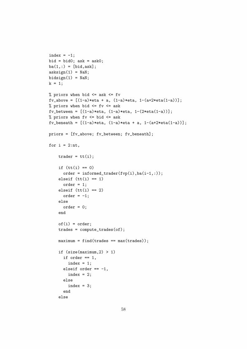
index = -1;

bid = bid0; ask = ask0;

ba(1,:) = [bid,ask];

asksign(1) = NaN;

bidsign(1) = NaN;

k = 1;

% priors when bid <= ask <= fv

fv_above = [(1-a)*eta + a, (1-a)*eta, 1-(a+2*eta(1-a))];

% priors when bid <= fv <= ask

fv_between = [(1-a)*eta, (1-a)*eta, 1-(2*eta(1-a))];

% priors when fv <= bid <= ask

fv_beneath = [(1-a)*eta, (1-a)*eta + a, 1-(a+2*eta(1-a))];

priors = [fv_above; fv_between; fv_beneath];

for i = 2:nt,

trader = tt(i);

if (tt(i) == 0)

order = informed_trader(fvp(i),ba(i-1,:));

elseif (tt(i) == 1)

order = 1;

elseif (tt(i) == 2)

order = -1;

else

order = 0;

end

of(i) = order;

trades = compute_trades(of);

maximum = find(trades == max(trades));

if (size(maximum,2) > 1)

if order == 1,

index = 1;

elseif order == -1,

index = 2;

else

index = 3;

end

else

58

index = maximum;

end

in(i) = index;

switch index,

case 1

if order == 1,

if (asksign(i-1) == 1)

k = 1;

end

ask = compute_ask(ba,i,delta_a,k);

bid = ba(i-1,1);

asksign(i) = 0;

bidsign(i) = bidsign(i-1);

else if order == -1,

if (bidsign(i-1) == 1)

k = 1;

end

bid = compute_bid(ba,i,delta_b,k);

ask = ba(i-1,2);

if (bid > ask)

bid = ask;

end

bidsign(i) = 0;

asksign(i) = asksign(i-1);

else

if (bidsign(i-1) == 1)

k = 1;

end

bid = compute_bid(ba,i,delta_b,k);

bidsign(i) = 0;

if (asksign(i-1) == 1)

k = 1;

end

ask = compute_ask(ba,i,delta_a,k);

asksign(i) = 0;

end

end

case 2

if order == 1,

59

if (asksign(i-1) == 0)

k = 1;

end

ask = compute_ask(ba,i,-delta_a,k);

bid = ba(i-1,1);

asksign(i) = 1;

bidsign(i) = bidsign(i-1);

if (ask < bid)

ask = bid;

end

else if order == -1,

if (bidsign(i-1) == 0)

k = 1;

end

bid = compute_bid(ba,i,-delta_b,k);

ask = ba(i-1,2);

bidsign(i) = 1;

asksign(i) = asksign(i-1);

else

if (bidsign(i-1) == 0)

k = 1;

end

bid = compute_bid(ba,i,-delta_b,k);

bidsign(i) = 1;

if (asksign(i-1) == 0)

k = 1;

end

ask = compute_ask(ba,i,-delta_a,k);

asksign(i) = 1;

end

end

case 3

if order == 1,

if (asksign(i-1) == 0)

k = 1;

end

ask = compute_ask(ba,i,-delta_a,k);

bid = ba(i-1,1);

asksign(i) = 1;

bidsign(i) = bidsign(i-1);

if (ask < bid)

ask = bid;

end

60

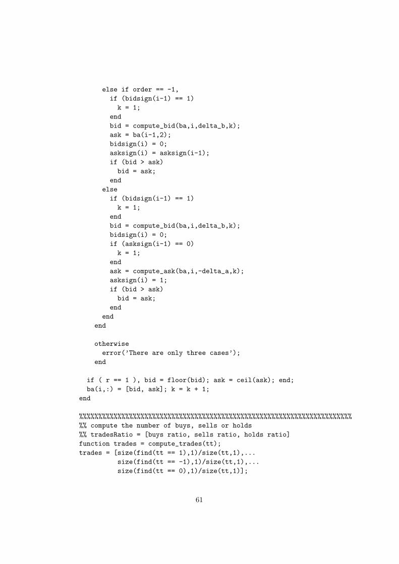
else if order == -1,

if (bidsign(i-1) == 1)

k = 1;

end

bid = compute_bid(ba,i,delta_b,k);

ask = ba(i-1,2);

bidsign(i) = 0;

asksign(i) = asksign(i-1);

if (bid > ask)

bid = ask;

end

else

if (bidsign(i-1) == 1)

k = 1;

end

bid = compute_bid(ba,i,delta_b,k);

bidsign(i) = 0;

if (asksign(i-1) == 0)

k = 1;

end

ask = compute_ask(ba,i,-delta_a,k);

asksign(i) = 1;

if (bid > ask)

bid = ask;

end

end

end

otherwise

error(’There are only three cases’);

end

if ( r == 1 ), bid = floor(bid); ask = ceil(ask); end;

ba(i,:) = [bid, ask]; k = k + 1;

end

%%%%%%%%%%%%%%%%%%%%%%%%%%%%%%%%%%%%%%%%%%%%%%%%%%%%%%%%%%%%%%%%%%%%%%%

%% compute the number of buys, sells or holds

%% tradesRatio = [buys ratio, sells ratio, holds ratio]

function trades = compute_trades(tt);

trades = [size(find(tt == 1),1)/size(tt,1),...

size(find(tt == -1),1)/size(tt,1),...

size(find(tt == 0),1)/size(tt,1)];

61

%%%%%%%%%%%%%%%%%%%%%%%%%%%%%%%%%%%%%%%%%%%%%%%%%%%%%%%%%%%%%%%%%%%%%%%%

%% Function to generate fundamental values to be used in the

% simulation

function fvp = generate_fvp(nsteps,v0,pj,sv);

jumps = [0;rand(nsteps-1,1) < pj]; jsize = sv*randn(nsteps,1);

fvp = v0 + cumsum(jumps .* jsize);

%%%%%%%%%%%%%%%%%%%%%%%%%%%%%%%%%%%%%%%%%%%%%%%%%%%%%%%%%%%%%%%%%%%%%%

%% Function to determine the order type for the informed trader

function order = informed_trader(fv,ba);

if ( fv > ba(2)),

order = 1; % buy

elseif ( fv < ba(1) ),

order = -1; % sell

else

order = 0; % hold

end

%% %%%%%%%%%%%%%%%%%%%%%%%%%%%%%%%%%%%%%%%%%%%%%%%%%%%%%%%%%%%%%%%%%%%%%%%%%%

function ask = compute_ask(ba,i,delta_a,k);

ask = ba(i-1,2) + (delta_a/k);

%% %%%%%%%%%%%%%%%%%%%%%%%%%%%%%%%%%%%%%%%%%%%%%%%%%%%%%%%%%%%%%%%%%%%%%%%%%%

function bid = compute_bid(ba,i,delta_b,k);

bid = ba(i-1,1) + (delta_b/k);

SimpleMM Code

for i = 2:nt,

trader = tt(i);

if (tt(i) == 0)

order = informed_trader(fv(i),ba(i-1,:));

elseif (tt(i) == 1)

order = 1;

elseif (tt(i) == 2)

order = -1;

else

order = 0;

end

of(i) = order;

62

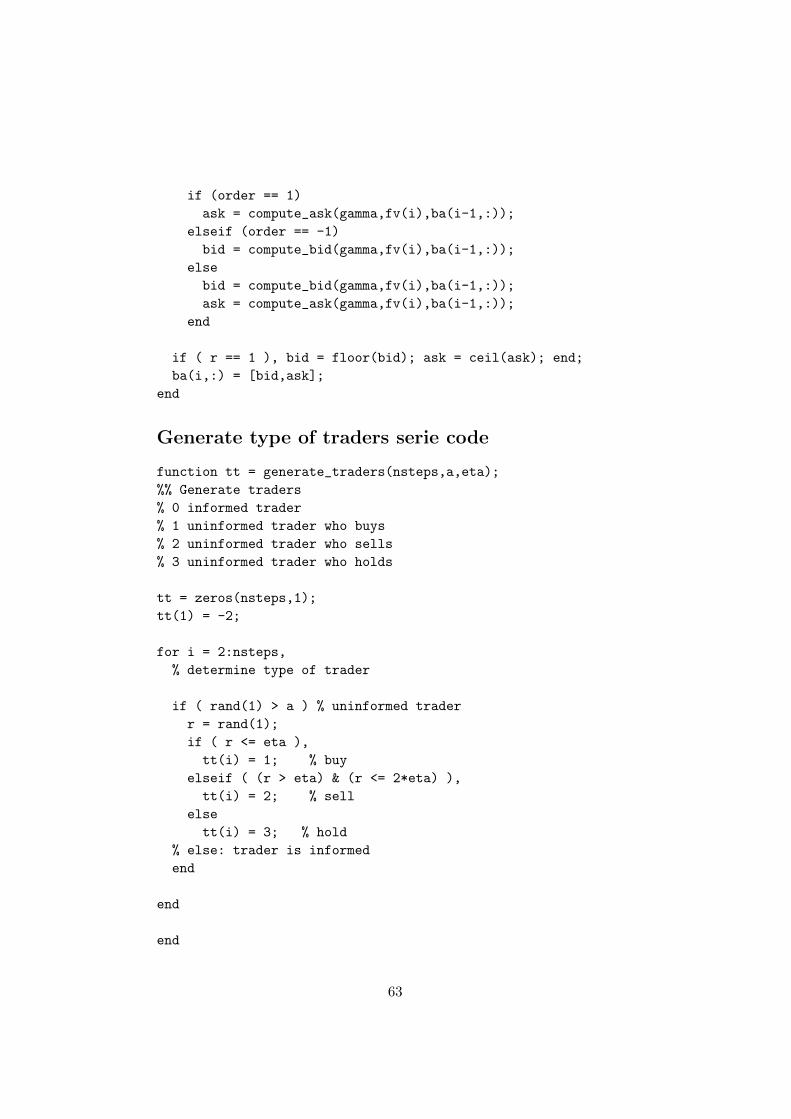
if (order == 1)

ask = compute_ask(gamma,fv(i),ba(i-1,:));

elseif (order == -1)

bid = compute_bid(gamma,fv(i),ba(i-1,:));

else

bid = compute_bid(gamma,fv(i),ba(i-1,:));

ask = compute_ask(gamma,fv(i),ba(i-1,:));

end

if ( r == 1 ), bid = floor(bid); ask = ceil(ask); end;

ba(i,:) = [bid,ask];

end

Generate type of traders serie code

function tt = generate_traders(nsteps,a,eta);

%% Generate traders

% 0 informed trader

% 1 uninformed trader who buys

% 2 uninformed trader who sells

% 3 uninformed trader who holds

tt = zeros(nsteps,1);

tt(1) = -2;

for i = 2:nsteps,

% determine type of trader

if ( rand(1) > a ) % uninformed trader

r = rand(1);

if ( r <= eta ),

tt(i) = 1; % buy

elseif ( (r > eta) & (r <= 2*eta) ),

tt(i) = 2; % sell

else

tt(i) = 3; % hold

% else: trader is informed

end

end

end

63

Different fundamental value with bid or ask pricecode

clear;

clc;

map = uigetdir;

dirListing = dir(map);

sumbid = 0;

sumask = 0;

meanba = ones(1000,2);

nsteps = 1000;

for i = 1:nsteps,

for d = 3:length(dirListing),

filename = dirListing(d).name;

load(filename);

sumbid = sumbid + ba(i,1);

sumask = sumask + ba(i,2);

end

meanba(i,1) = sumbid / 100;

meanba(i,2) = sumask / 100;

sumbid = 0;

sumask = 0;

end

diffbid = sum(abs(fv - meanba(:,1)));

diffask = sum(abs(meanba(:,2) - fv));

diffmean = (diffbid + diffask) / 2;

Calculate mean 100 simulations to plot

clear;

clc;

map = uigetdir;

dirListing = dir(map);

sumbid = 0;

sumask = 0;

64

meanba = ones(1000,2);

nsteps = 1000;

for i = 1:nsteps,

for d = 3:length(dirListing),

filename = dirListing(d).name;

load(filename);

sumbid = sumbid + ba(i,1);

sumask = sumask + ba(i,2);

end

meanba(i,1) = sumbid / 100;

meanba(i,2) = sumask / 100;

sumbid = 0;

sumask = 0;

end

Calculate the mean sum of bid-ask spreads

clear;

clc;

map = uigetdir;

dirListing = dir(map);

for d = 3:length(dirListing),

filename = dirListing(d).name;

load(filename);

meanba(d) = sum((ba(:,2) - ba(:,1))) / size(ba,1);

end

65

Bibliography

[1] L. Glosten abd P. Milgrom. Bid, ask and transaction orices in a special-ist market with heterogeneously informed traders. Journal of FinancialEconomics, 14(1):70–100, 1985.

[2] A.R. Admati and P. Pfleiderer. A theory of intraday patterns: volumeand price variability. The Review of Financial Studies, 1(1):2–40, 1988.

[3] Y. Amihud and H. Mendelson. Dealership market: market making withinventory. Journal of Financial Economics, 8(1):31–53, 1980.

[4] L. Glosten B. Biais and C. Spatt. Market microstructure: A survey ofmicrofoundations, empirical results, and policy implications. Journalof Financial Markets, 8:217–264, 2005.

[5] W. Bagehot. The only game in town. Financial Analysts Journal,27(2):12–14,22, 1971.

[6] M. Brunnermeier. Asset pricing under asymmetric information: bub-bles, crashes, technical analysis, and herding. Oxford University Press,2001.

[7] Nicholas T. Chan and Christian R. Shelton. An electronic market-maker. In Seventh International Conference of the Society for Compu-tational Economics, 2001.

[8] N.T. Chan. Artificial markets and intelligent agents. PhD thesis, Mas-sachusetts Institute of Technology, 2001.

[9] M. Chhabra and S. Das. Learning the demand curve in posted-price dig-ital to market auctions. In Proceedings of the Tenth International JointConference on Autonomous Agents and Multi-Agent System, pages 63–70, 2011.

[10] S. Das. Intelligent market-making in artificial financial markets. Mas-ter’s thesis, Department of Electical Engineering and Computer Sci-ence, Massachusetts Institute of Technology, 2003.

66

[11] S. Das. A learning market maker in the glosten-milgrom model. Quan-titative Finance, 5(2):169–180, 2005.

[12] S. Das. Learning to trade with insider information. In Proceedings ofthe Ninth International Conference on E-Commerc, 2007.

[13] S. Das. The effects of market-making on price dynamics. In Proceedingsof the Seventh International Joint Conference on Autonomous Agentsand Multi-Agent System, pages 997–894, 2008.

[14] S. Das and M. Magdon-Ismail. Adapting to a market shock: Optimalsequential market-making. In Advances in Neural Information Process-ing Systems 21, pages 361–368, 2009.

[15] S. Das and M. Magdon-Ismail. Comparing prediction market structures,with an application to market making. Quantitative Finance PapersarXiv.org, 2010.

[16] F.D. Foster and S. iswanathan. Strategic trading when agents forecastthe forecasts of others. Journal of Finance, 51(4):1437–1478, 1996.

[17] M. Garman. Market microstructure. Journal of Financial Economics,3(3):257–275, 1976.

[18] T. Ho and H. Stoll. Optimal dealer pricing under transactions andreturn uncertainty. Journal of Financial Economics, 9(1):47–73, 1981.

[19] T. Ho and H. Stoll. The dynamics of dealer markets under competition.Journal of Finance, 38(4):1053–1074, 1983.

[20] C.W. Holden and A. Subrahmanyam. Long-lived private informationand imperfect competition. Journal of Finance, 47(1):247–270, 1992.

[21] F. De Jong and B. Rindi. The Microstructure of Financial Markets.Cambridge University Press, 2009.

[22] A. Kyle. Continuous auctions and insider trading. Econometrica,53(6):1315–1336, 1985.

[23] A. Kyle. Informed speculation with imperfect competition. Review ofEconomic Studies, 56:317–355, 1989.

[24] A. Madhaven. Market microstructur: a survey. Journal of financialmarkets, 3(3):205–258, 2000.

[25] A. Madhaven. Market microstructur: a practioner’s guide. FinancialAnalysts Journal, 58(2):1–28, 2002.

[26] M. O’Hara. Market Microstructure Theory. Blackwell Publishers, 2000.

67

[27] C. Parlour and D. Seppi. Limit order markets: A survey. Handbook ofFinancial Intermediation and Banking, 2008.

[28] R.A. Schwartz. Reshaping the equity markets: a guide for the 1990s.HarperBusiness, 1991.

[29] S. Smidt. The road to an efficient stock market. Financial AnalystsJournal, 27:18–20, 64–69, 1971.

[30] H.R. Stoll. The supply of dealer services in securities markets. Journalof Finance, 33(4):1133–1151, 1978.

[31] S. Tinic and R. West. Competition and the pricing of dealer servicesin the over-the-counter market. Journal of Financial and QuantitativeAnalysis, 8:1707–1727, 1972.

68