Ecology of Freshwater Fish 2002: 11: 2–10 Copyright C Blackwell Munksgaard 2002Printed in Denmark ¡ All rights reserved

ISSN 0906-6691

A new optimal foraging model predictshabitat use by drift-feeding stream minnows

Grossman GD, Rincon PA, Farr MD, Ratajczak, RE, Jr. A new optimal G. D. Grossman1, P. A. Rincon2,foraging model predicts habitat use by drift-feeding stream minnows. M. D. Farr*, R. E. Ratajczak Jr1

Ecology of Freshwater Fish 2002: 11: 2–10.C Blackwell Munksgaard, 2002 1D. B. Warnell School of Forest Resources,University of Georgia, Athens, Georgia, USA, and

Abstract – There is substantial need for models that accurately predict 2Departamento de Ecologia Evolutiva, Museohabitat selection by fishes for purposes ranging from the elaboration of Nacional de Ciencias Naturales, C.S.I.C, C/. Joseecological theory to the preservation of biodiversity. We have developed a Gutierrez Abascal 2, Madrid, Spainnew and highly tractable optimal foraging model for drift-feeding fishes *Current address: US Army Corps of Engineers,

St Paul, Minnesota, USAthat is based on the profitability of occupying varying focal-pointvelocities in a stream. The basic model can be written as: Ix Ω (Ex * Px) Ω(D * A * V) * [1/(1 π e(b π cV))] ª Sx, where: (1) Ix is the net energy intakeat velocity x; (2) E is prey encounter rate; (3) P is prey capture successrate which can be modelled as 1/(1 π e(b π cV)) where b and c are fittingconstants from the prey capture success curve; (4) D is the energy contentof prey (J/m3) in the drift; (5) A is the visual reactive area of the fish; (6)V is velocity (cm/s); and (7) S is the cost of maintaining position (J/s).Given that D, A and S can be considered constant over the range ofvelocities occupied by these fishes, the model reduces to e(b π cV) Ω 1/(cV ª1) which we solved iteratively to yield an optimal focal-point velocity forspecies in each sample. We tested the model by comparing its predictionsto the mean focal-point velocities (i.e. microhabitats) occupied by fourspecies of drift-feeding minnows in two sites in a stream in NorthCarolina, USA. The model successfully predicted focal-point velocitiesoccupied by these species (11 out of 14 cases) in three seasonal samplescollected over 2 years at two sites. The unsuccessful predictions still werewithin 2 cm/s of the 95% confidence intervals of mean velocities occupiedby fishes, whereas the overall mean deviation between optimal velocitiesand mean fish velocities was small (range Ω 0.9 and 3.3 cm/s for thewarpaint shiner and the Tennessee shiner, respectively). Available focal-point velocities ranged from 0–76 to 0–128 cm/s depending on site andseason. Our findings represent one of the more rigorous field tests of anoptimal foraging/habitat selection model for aquatic organisms becausethey encompass multiple species and years, and for one species, multiple Key words: cost-benefit; focal-point velocity;sites. Because of the ease of parameterization of our model, it should be foraging success; IFIM; interspecific

competition; microhabitat; optimization; streamreadily testable in a range of lotic habitats. If validated in other systems,fishes; TMDLthe model should provide critical habitat information that will aid in the

management of riverine systems and improve the performance of a Gary D. Grossman, D. B. Warnell School ofForest Resources, University of Georgia,variety of currently used management models (e.g. instream flowAthens, Georgia, USAincremental methodology (IFIM) and total maximum daily load

calculations (TMDL)). Accepted for publication October 22, 2001

Un resumen en espanol se incluye detras del texto principal de este artıculo.

Introduction

The question of why animals prefer certain habi-tats and avoid others has intrigued ecologists andnatural historians for millennia. In fact, over the

2

past 50years, the construction and testing of syn-thetic models of habitat selection have been crucialto theoretical advancement in ecology, ethology,and fisheries science (Stephens & Krebs 1986; Pul-liam 1989; Wootton 1999). Although the study of

Optimal foraging in stream fishes

habitat selection has its roots in basic ecology andethology, there also are strong societal needs formodels that elucidate the mechanisms determininghabitat selection in aquatic organisms. For ex-ample, such models are essential for the preser-vation of aquatic biodiversity, which has beenstrongly affected by the continued alteration anddegradation of aquatic habitats (Moyle & Cech2000). Such degradation will probably increase asanthropogenic disturbances such as (1) im-poundments (Hill 1996), (2) non-point source pol-lution [e.g. total maximum daily load (TMDL);http://www.epa.gov/owow/tmdl/proprule.html] and(3) global climate change (Meyer et al. 1999) con-tinue to increase.

Despite these compelling scientific and societalneeds, the majority of models currently used to as-sess habitat requirements for fishes are based oncorrelative analyses of fish abundance data andphysical habitat variables, rather than on identifi-cation of the specific mechanisms underlying habi-tat selection by fishes (Grossman et al. 1995;Baker & Coon 1997). For example, many streamfishes preferentially occupy high-velocity micro-habitats and reaches (Grossman & Ratajczak1998; Matthews 1998; Thompson et al. 2001), butfew correlational studies enable us to deduce thereason behind this pattern (e.g. Do these reacheshave higher prey availability? Do they offer greaterprotection from predators? Do they provide essen-tial spawning habitat?). This shortcoming limitsboth our basic understanding of the process ofhabitat selection in fishes as well as our ability toscientifically manage these species.

In contrast to correlational techniques, optimalforaging theory is a mechanistic approach that canbe used to predict habitat selection by animals viathe assumption that natural selection will produceindividuals that behave in a manner that maxim-izes individual fitness (Stephens & Krebs 1986; Ro-senzweig & Abramsky 1997). Although fitness isthe currency of optimal foraging theory, it gener-ally is not measured directly because of the logis-tical difficulties inherent in measuring reproductivesuccess (number of offspring surviving) especiallyfor fishes. Consequently, many investigators testhabitat selection predictions of optimal foragingtheory using parameters that are generally con-sidered to be strongly correlated with fitness; forexample, net energy intake (Werner & Hall 1979;Hill & Grossman 1993; Wootton 1999). A re-searcher can then determine whether specimens arebehaving in concordance with the predictions ofoptimal foraging theory by examining whetherthey occupy microhabitats that maximize their netrate of energy intake, although constraints such aspredator avoidance and nutrient limitation may

3

need to be included in analyses (Stephens & Krebs1986; Gilliam & Fraser 1987; Pulliam 1989). Suchapproaches have been successfully used to predictmicrohabitat selection for several fish species(Fausch 1984; Dill 1987; Hughes & Dill 1990;Hill & Grossman 1993; Hughes 1998). Thesestudies, which have focused on drift-feedingstream salmonids, all have shown that focal-pointvelocity (i.e. velocity at the position of the fish; seeGrossman & Freeman 1987) is a crucial compo-nent of optimal habitat selection.

In this report, we present a new and highly trac-table optimal foraging model that successfully pre-dicts the microhabitats (i.e. focal-point velocities)occupied by four species of drift-feeding minnows(family cyprinidae) in a stream in North Carolina,USA. Our study species were rosyside dace, Clinos-tomus funduloides Girard; warpaint shiner, Luxiluscoccogenis (Cope); Tennessee shiner, Notropis leu-ciodus (Cope); and yellowfin shiner, Notropis lutip-innis (Jordan & Brayton). One of these species,rosyside dace, is a species of special concern(NCWRC Year?). Minnows are the most abundantfreshwater fish taxon world-wide, with the excep-tion of South America and Australia (Moyle &Cech 2000), and drift-feeding minnows are fre-quently the most diverse and abundant fish taxonin lotic systems (Matthews 1998). Consequently,our model may be applicable to a large number ofspecies found over a broad geographical range. Inaddition, our findings represent a relatively rigor-ous field test of an optimal foraging/habitat selec-tion model because they encompass multiple spe-cies and years, and for one species, multiple siteswithin a stream.

Materials and methodsModel

As discussed previously, a habitat selection modelbased on optimal foraging theory should predictthat drift-feeding fishes will occupy focal-pointvelocities (all further references to fish velocities re-fer to focal-point velocity) that maximize the fish’snet rate of energy intake (Fausch 1984; Hughes &Dill 1990; Hill & Grossman 1993; Hughes 1998).For drift-feeding fishes, the rate of energy intake isa function of: (1) V, velocity (cm/s); (2) A, the vis-ual reactive area of the fish (as per Hughes & Dill1990; Hughes 1998), where A is the area of a trans-verse section (cm2) through the reactive volume ofthe fish (ideally, a sphere whose radius is the maxi-mum distance at which the fish can visually detectprey) taken at its head; and (3) D, the energy con-tent of prey (J/m3) in the drift. Given that D is notdependent on V within a given pool or riffle (Al-lan & Russek 1985; Matthaei et al. 1998), then E,

Grossman et al.

the prey encounter rate [i.e. the rate at which Dcrosses A (J/s)] is linearly related to V as EΩD*A*V (Hughes 1998). Energy intake is also a functionof the prey capture success of the fish (P, the pro-portion of prey crossing A that are captured) andthe cost of maintaining position [S (J/s)] at a givenvelocity. The relationship between P and velocity(see Hill & Grossman 1993) can best be describedby:

P Ω 1/(1 π e(b π cV)) (1)

where b and c are fitting constants. We have pre-viously shown that swimming costs are small andrelatively constant within the range of velocities forwhich P.0 (Facey & Grossman 1990); conse-quently, net energy intake (I) at velocity x can beexpressed as:

Ix Ω (Ex *Px)Ω (D*A*V) * [1/(1 π e(b π cV))] ª Sx (2)

and fishes should occupy the velocity that maxim-izes I. We derived a value for this velocity by solv-ing dI/dVΩ0 for V. Given that D, A and S canbe considered constant over the range of velocitiesoccupied by these fishes (Facey & Grossman 1990;Hughes & Dill 1990; q4'Hill & Grossman 1993), weobtain:

e(b π cV) Ω 1/(cV ª 1) (3)

which we solved iteratively to yield an optimal fishvelocity. The significance of this finding is that de-termination of optimal velocity depends only uponthe readily obtained parameters b and c of the preycapture success curve (i.e. P versus V), rather thanon A or S, which are quite difficult to measure(Hill & Grossman 1993).

Experimental procedures

We constructed prey capture success curves (i.e.obtained values for parameters b and c for ourmodel) using field and experimental methods simi-lar to those of Hill & Grossman (1993). In brief,we captured fishes during 1998 in Coweeta Creek,Macon County, NC, USA, (general site descrip-tion in Hill & Grossman 1993) at water tempera-tures of 18–20 æC. Fishes were returned to the lab-oratory and held in tanks at 18 æC and water velo-cities of approximately 5cm/s for 2–3days beforebeing used in prey capture success trials (con-ducted at 18 æC). Prior to experiments, we fed thefishes trout chow pellets (,1.5mm in diameter)and live Hyalella azteca (Amphipoda, 4–7mm inlength) at levels which approximated a mainten-ance ration (Hill & Grossman 1993).

We conducted prey capture success trials in afibreglass artificial stream equipped with a Plexigl-

4

as viewing window. The stream was 183cm long by91.5cm wide by 35.5cm deep, and was partitionedwith mesh screen and Plexiglas into a test chamber90cm long by 35cm wide by 35.5cm deep. Wemarked both the sides and bottom of the testchamber with grids to facilitate identification ofthe exact position of a specimen during trials. Toreduce disturbance, we made observations frombehind a black plastic blind. We maintained waterflow in the test chamber with a continuously vari-able speed 12-V motor (thrustΩ16.8kg) whichdrove a propeller positioned at the front of thestream. A honeycomb collimator placed betweenthe motor and the test chamber produced laminarflow (i.e. Re Ω400) throughout the chamber. Al-though drift-feeding fishes live in environmentsthat contain turbulence, the introduction of small-scale turbulence into prey capture experimentswould have made accurate velocity measurementsintractable.

We began a trial by presenting live H.azteca (4–7mm long) to test specimens via a piece of flexibleplastic tubing (3mm inside diameter) attached toa screen bounding the upstream portion of the testchamber (delivery depth 5cm from the water’s sur-face). Individual prey were placed in the water-filled tube and delivered by opening a clamp, whichreleased the amphipod into the current. A series ofpilot experiments enabled us to track the typicaltrajectory of prey in the test chamber and we ad-justed the motor to produce treatment velocities(at the fishes focal position) ranging from 5 to 40cm/s (5-cm/s intervals). We used live H.azteca inprey capture success trials because: (1) fishes fedon H.azteca using foraging behaviours similar tothose displayed when foraging on native prey(Freeman & Grossman 1992; G. Grossman, per-sonal observation); (2) at all test velocities, H.azte-ca remained in the water column throughout thelength of the test chamber; and (3) in contrast toprey found in Coweeta Creek, H.azteca were read-ily cultured. This species is not found in driftsamples from Coweeta Creek; however, amphipodsare important components of drift in manystreams (Brittain & Eikeland 1988).

We ascertained that a test subject would feed byfirst placing it in the test chamber and giving it 10min to acclimate at 10cm/s, and then deliveringprey until it made one capture. (The few specimensthat refused to feed were not used in trials.) Theapparatus was then gradually adjusted until treat-ment velocity was reached (treatment velocitieswere calculated at the position of the fishes to per-mit tests using field fish velocity measurements).We then began releasing individual prey at ap-proximately 20-s intervals until 10 prey were de-livered while an observer tabulated the total num-

Optimal foraging in stream fishes

ber of prey captured. During trials, we recordedboth the focal position occupied by a fish prior toa strike as well as the location of each prey strike.After completion of a trial, we measured velocities(∫0.1cm/s) at these locations using an electromag-netic flow meter (Hill & Grossman 1993). We con-ducted trials using solitary fish between 0900 and1930h and each subject was tested at two or threevelocities in a given day in an order that minimizedthe effects of satiation and fatigue. Trials were con-ducted during daylight hours because these speciesforage throughout the day and generally becomequiescent at night (Freeman & Grossman 1992;Hill & Grossman 1993; G. Grossman et al., per-sonal observation).

We derived species-specific prey capture successcurves from: (1) 28 rosyside dace (35–68mm, alllengths represent standard length), 29 warpaintshiners (31–100mm), 26 Tennessee shiners (33–58mm) and 23 yellowfin shiners (44–69mm). Becausefish size affects both the prey capture success(Hill & Grossman 1993) and velocity use of fishesin streams (Grossman & Ratajczak 1998), we de-veloped separate prey capture success curves forup to three size classes for each species. We fitcurves using equation 1 and the Statistica non-lin-ear least squares regression computer program(StatSoft, Inc., Tulsa, OK, USA).

Field test

We tested predictions of our model through com-parison with mean fish velocities utilized by thefour species in Coweeta Creek (site 4) during July1996, and June and August 1997. In addition, wetested model predictions for rosyside dace at a sec-ond site (same months, site 1) where it was the onlydrift-feeding cyprinid present. These sites weretypical of fifth-order streams within the region andhad mixed substrata dominated by boulder, cobbleand gravel (site 4Ω71%; site 1Ω86%). Nonethe-less, depositional substrata (e.g. sand, silt anddebris) also were present within both sites. Themean depths of the sites were 22cm (site 1) and 25cm (site 4), and the mean velocities for the sam-pling periods are presented in the ‘Results’ below.Geographically, site 1 was slightly upstream fromthe study reach of Grossman et al. (1998) and thesite 4 was approximately 1.2km downstream.

We tested our model using each species bysample by site combination (nΩ14). We measuredboth fish velocities and mean water column velo-cities (100 random measurements) available ineach site during each sample period using standardmethods Grossman & Freeman 1987; Grossman &Ratajczak 1998; Grossman et al. 1998). We ob-tained predicted optimal velocities from our model

5

using equation 3 and the prey capture successcurve parameters (i.e. b and c) for each fish sizeclass. We solved equation 3 for each size class iter-atively using the Solver (quasi-Newton) algorithmof the Excel 97 computer program (Microsoft Inc.,Redmond, WA, USA). Then we sorted field fishvelocity measurements into size classes andweighted predicted optimal velocities by size-speci-fic model values (i.e. if a field sample contained 10velocity observations for fish between 50 and 60mm, and eight observations for fish . 60mm, wecalculated an optimal velocity by multiplying theprediction for 50–60mm fish by 10 and the predic-tion for.60mm fish by eight, summed the total,and then divided by 18). Field observations of fishvelocities included individuals in the following sizeclasses: (1) rosyside dace (50–70mm); (2) warpaintshiner ($80mm); (3) yellowfin shiner (50–60mm);and (4) Tennessee shiner (50–60mm). Because wecould not obtain exact size duplicates for both fishvelocity measurements and prey capture successcurves, we excluded some specimens/curves fromanalyses. Our model produced a single value foroptimal velocity, and consequently, we evaluatedeach prediction statistically by determiningwhether or not it fell within the 95% confidenceinterval (CI) for a particular field fish velocitysample mean (Johnson 1999). If a prediction fellwithin the 95% CI, then the model successfully fitthe data, whereas predictions that fell outside the95% CI were considered unsuccessful (Johnson1999).

We have previously shown that the velocity atwhich the third derivative of the prey capture suc-cess curve reached zero (i.e. the point of maximumdeceleration of the curve; see Hill & Grossman1993) was a good predictor of velocities occupiedby rainbow trout, Oncorhynchus mykiss (Wal-baum), and rosyside dace in Coweeta Creek.

Fig.1. A prey capture success curve for rosyside dace (56–68mm SL, nΩ13) which is representative of the curves describedin Table I. All curves had very high R2 values (meanΩ90%,rangeΩ81–96%); hence, we did not plot the individual points.

Grossman et al.

Consequently, we also compared predictions basedon the third derivative of prey capture successcurves to field fish velocities. We then comparedthe number of successful predictions of the thirdderivative to those of our new model to ascertainwhich model yielded the greatest number of suc-cessful predictions for field data.

Results

The prey capture success curves were non-linearfor all species (Fig.1) and best fit by equation 3(Hill & Grossman 1993). These curves explained avery high amount of variance in the data, with amean R2 value of 0.90 (rangeΩ0.81–0.96, ‘all size-class’ regressions omitted, see Table I). The rangeof velocities present in the Coweeta Creek sitesduring field tests was substantial and varied from0–76cm/s to 0–128cm/s (Figs2–5). None of thesample means for velocity availability data fellwithin the 95% CI of mean fish velocities, demon-strating that fishes did not occupy velocities at ran-dom (Figs2–5). Despite the wide range of velo-

Fig.2. Optimal velocities (*) predicted by the model, mean observed fish velocities (O) and 95% confidence interval (CI), and meanwater column velocities available within site 4 during July 1996. The mean of mean water column velocity measurements is shownby l. All model predictions were successful (i.e. they fell within the 95% CI of mean fish velocities). We made fish measurementson 3, 6 and 8 July, and habitat availability measurements within two weeks of fish measurements. Predictions for the alternativemodel of Hill & Grossman (1993), i.e. the third derivative of the prey capture success curve, were as follows: rosyside dace, 13.9cm/s; warpaint shiner, 13.4cm/s; yellowfin shiner, 11.8cm/s; and Tennessee shiner, 11.0cm/s. Predictions of the alternative model failedfor both rosyside dace and Tennessee shiner.

6

Table 1. Model parameters for prey capture success curves. Curves were fitwith the following equation: P Ω 1/(1 π e (b π cV)), where P is prey capturesuccess, V is velocity, and b and c are fitting constants. All regressions weresignificant at P # 0.01.

Species Size class n b c R 2

(SL, mm)

Rosyside dace All 28 ª3.956 0.215 0.8335–41 5 ª3.302 0.249 0.8144–52 10 ª4.299 0.237 0.9356–68 13 ª4.393 0.214 0.87

Warpaint shiner All 29 ª4.027 0.258 0.8631–42 7 ª4.112 0.366 0.9349–65 13 ª4.576 0.288 0.9170–100 9 ª4.682 0.251 0.96

Tennessee shiner All 26 ª3.730 0.282 0.8233–47 15 ª4.548 0.407 0.8750–58 11 ª4.154 0.257 0.87

Yellowfin shiner All 23 ª4.091 0.234 0.9244–52 7 ª4.006 0.224 0.9055–69 16 ª4.137 0.239 0.93

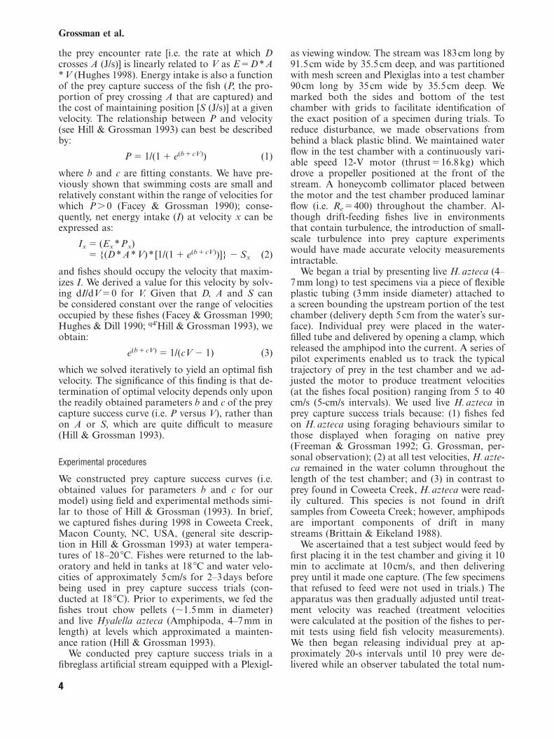
cities available, our model successfully predictedfish velocities in Coweeta Creek in 11 out of 14cases (79%; Figs2–5). In addition, even the three

Optimal foraging in stream fishes

unsuccessful predictions lay within 2cm/s of the95% CI (Figs2–5). Finally, our new model was abetter predictor of fish velocities in Coweeta Creekthan the third derivative (11 out of 14 successfulpredictions versus nine out of 14; Figs2–5).

Discussion

Our results indicate that an optimal foragingmodel can be used to predict the focal-point velo-cities occupied by several species of stream min-now, and it is likely that optimization theory willcontinue to be an efficacious tool for understand-ing habitat selection in fishes (Werner & Hall 1979;Persson 1990; Grand & Grant 1994; Tyler & Gilli-am 1995; Grand 1997). In addition, this model hasseveral advantages over previous models including:(1) its mechanistic basis (i.e. it is likely thatmeasuring prey capture success at different focal-point velocities actually quantifies a factor crucialto microhabitat selection); (2) it is based on a cur-rency (i.e. maximization of energy intake) which isprobably strongly correlated with individual fit-ness; and (3) it is highly tractable and easily par-ameterized (i.e. there is no need to estimate D, Sand A). The tractability and ease with which model

Fig.3. Optimal velocities (*) predicted by the model, mean observed fish velocities (O) and 95% confidence interval (CI), and meanwater column velocities available within site 4 during June 1997. The mean of mean water column velocity measurements is depictedby l. Only the model prediction for yellowfin shiner fell outside of the 95% CI of mean fish velocities (i.e. model failure). We madefish measurements on 25 and 26 June, and habitat availability measurements on 31 May. Predictions for the alternative model ofHill & Grossman (1993) were as follows: rosyside dace, 13.9cm/s; warpaint shiner, 13.4cm/s; and yellowfin shiner, 11.8cm/s. Theprediction of the alternative model fell outside the 95% CI of mean fish velocities for rosyside dace (i.e. the alternative model failed).

7

parameters can be obtained through relativelysimple experiments provide a stark contrast to theextensive laboratory work required for the con-struction of energy-based cost–benefit models (Fa-cey & Grossman 1990; Hill & Grossman 1993).

Although the model success rate was not 100%(i.e. 79%), sample sizes for some analyses were low(i.e. ,15 individuals), and experimental tempera-tures were higher (18 æC) than many field fish velo-city measurements (i.e. made between 15.9 and 18.3æC). However, the agreement between most modelpredictions and 95% CIs of velocities occupied byfishes in Coweeta Creek is particularly noteworthybecause the 95% CIs were relatively small (meanΩ5.9cm/s), especially when compared to the range ofvelocities available in the creek (i.e. between 78 and128cm/s, depending on season). In addition, devi-ations between the optimal velocity predicted by themodel and mean velocities occupied by fishes in Co-weeta Creek were also small, ranging from 0.9cm/s(warpaint shiner) to 3.3cm/s (Tennessee shiner). Infact, even unsuccessful predictions were very closeto the boundaries of successful predictions (i.e.within 2cm/s of 95% CIs). These results suggest thatour model was a robust predictor of fish microhabi-tat selection in Coweeta Creek.

Grossman et al.

Fig.4. Optimal velocities (*) predicted by the model, mean observed fish velocities (O) and 95% confidence interval (CI), and meanwater column velocities available within site 4 during August 1997. The mean of mean water column velocity measurements isdepicted by l. Model predictions for rosyside dace and Tennessee shiner fell outside of the 95% CI of mean fish velocities (i.e.model failure). We made fish measurements on 12 and 16 August, and habitat availability measurements within two weeks of thesedates. Predictions for the alternative model of Hill & Grossman (1993) were as follows: rosyside dace, 13.9cm/s; warpaint shiner,13.4cm/s; yellowfin shiner, 11.8cm/s; and Tennessee shiner, 11.0cm/s. Predictions of the alternative model fell outside of the 95%CI of mean fish velocities for both warpaint shiner and Tennessee shiner (i.e. the alternative model failed).

The finding that Coweeta Creek fishes typicallyoccupied ‘optimal velocities’ also supports previousconclusions that habitat selection by fishes in thissystem is not strongly affected by either interspecificcompetition or predation (Grossman et al. 1998).Such results may not pertain to other lotic systems(Power et al. 1985; Gilliam & Fraser 1987; Schlosser1987), although it is clear that fish assemblages withcharacteristics similar to those of Coweeta Creekare not uncommon (Harvey & Stewart 1991; Mat-thews 1998). If our model is validated on a broaderscale it is possible that it will be useful as a heuristictool (via unsuccessful predictions) to identify sys-tems in which habitat selection is dominated by pro-cesses other than energy maximization (e.g. pre-dation or interspecific competition).

The simplicity and tractability of our model willprobably facilitate its use for a variety of purposes.For example, it may prove useful in identifying es-sential habitat characteristics (i.e. focal-point velo-city) for threatened/endangered species or for trop-ical species for which ecological information gen-erally is lacking. Data from our model also can bedirectly inserted into hydrologically based manage-

8

ment models (e.g. PHABSIM; Bovee 1982) that arecurrently utilized to estimate the potential biologi-cal and physical impacts of impoundments andwater diversions on lotic systems.

In conclusion, our model proved highly success-ful in predicting habitat selection over multipleyears by four species of stream cyprinids: membersof perhaps the most widespread and speciose fam-ily of freshwater fishes. Nonetheless, the generalityand robustness of the model now need to be as-sessed in a diversity of habitats. For example, itmay be necessary to modify several simplifying as-sumptions (e.g. the independence of D and V, andthe independence of D and habitat type) to achievesuccessful predictions for non-cyprinid drift feed-ers or for species in other systems. In addition, al-though our model predictions were empirically de-rived, they happened to fall within a relativelysmall range of velocities (see Figs2–5), whichlimited the strength of our conclusions. Neverthe-less, if the model is validated in other systems, itshould become a highly efficacious tool for boththe study of habitat selection and the managementof aquatic organisms across a range of habitats.

Optimal foraging in stream fishes

Fig.5. Optimal velocities (*) predictedby the model, mean observed fish veloci-ties (O) and 95% confidence interval (CI)for rosyside dace, and mean water co-lumn velocities available within site 1during July 1996, June 1997 and August1997. The mean of mean water columnvelocity measurements is depicted by l.All model predictions fell within the 95%CI of mean fish velocities. We made fishmeasurements on 2 and 4 July 1996, 23June 1997, and 13 and 15 August 1997,and habitat availability measurements inJuly 1996, June 1997 and August 1997(See Figs 2–4). The prediction of the al-ternative model of Hill & Grossman(1993), i.e. the third derivative of theprey capture success curve, was 14.4cm/s for all three samples and all fell withinthe 95% CI of mean fish velocities.

Resumen

1. Existe una grave necesidad de modelos que predigan conprecision la seleccion de habitat por parte de los peces con finesque van del desarrollo de la teorıa ecologica a la conservacionde la biodiversidad. Nosotros hemos desarrollado un modelonuevo y de facil manejo de alimentacion optima para peces quese alimentan de la deriva que se fundamenta en los diferentesbeneficios energeticos derivados de ocupar velocidades focalesdistintas en un rıo.2. El modelo basico puede formularse como: Ix Ω (Ex *Px)Ω(D*A*V) * [1/(1πe(b π cV))]ªSx, donde: (1) Ix es el energıaneta obtenida a la velocidad, x; (2) V es la velocidad (cm/s); (3)A es el area visual de reaccion del pez; (4) D es la energıa conte-nida en las presas (J/m3) en la deriva; (5) E es la tasa de encuen-tro de presas; (6) P es la probabilidad de captura de la presa,que puede representarse como 1/(1πe(b π cV)) donde b y c sonconstantes; y (7) S es el coste de nadar para mantener la posi-

9

cion en la corriente (J/s). Puesto que D, A y S pueden conside-rarse constantes en el rango de velocidades que ocupan estospeces, el modelo se reduce a e(b π cV) Ω1/(cVª1) que resolvimositerativamente para obtener una velocidad focal optima paracada especie en cada muestreo.3. Probamos el modelo comparando su predicciones con la ve-locidades focales medias (i.e. microhabitats) ocupadas por cua-tro especies de ciprınidos que se alimentan de la deriva en unrıo de Carolina del Norte. El modelo predijo con exito las velo-cidades focales ocupadas por estas especies (11/14 casos) en tresmuestreos estacionales llevados a cabo a lo largo de dos anosen dos estaciones. Incluso las predicciones fallidas se diferencia-ron en menos de 2cm/s del lımite de confianza al 95% CIs delas velocidades medias ocupadas, y la diferencia media entrepredicciones y observaciones fue pequena (rango Ω 0.9cm/swarpaint shiner, a 3.3-cm/s Tennessee shiner). El rango de lasvelocidades focales medias disponibles fue de 0–76cm/s a 0–128cm/s dependiendo de la localidad y estacion del ano.4. Nuestros resultados son una de las pruebas de campo mas

Grossman et al.

rigurosas de un modelo de alimentacion optima/seleccion dehabitat para organismos acuaticos puesto que incluyen diversasespecies, anos y, para una de las especies, localidades. La facili-dad de la estima de los parametros del modelo hace que seafacil probarlo en diversos habitats loticos. Si es validado enellos, el modelo deberıa proporcionar informacion valiosa queayudara a la gestion de los sistemas fluviales y mejorara losresultados obtenidos a traves de varios modelos usados actual-mente para la gestion (p.e. IFIM y calculos TMDL).

Acknowledgements

This research was funded by USDA McIntire-Stennis grantGEO-0086-MS, National Science Foundation grant BSR-9011661 and the Warnell School of Forest Resources. We aregrateful for the comments of R. Cooper, R Jackson, N. Lamou-roux, S. McCutcheon, J. Peterson, D. Promislow, R. Pulliamand J. Tyler.

References

Allan, J.D. & Russek, E. 1985. The quantification of streamdrift. Canadian Journal of Fisheries and Aquatic Sciences42: 210–215.

Baker, E.A. & Coon, T.G. 1997. Development and evaluationof alternative habitat suitability criteria for brook trout.Transactions of the American Fisheries Society 126: 65–76.

Bovee, K. 1982. A guide to stream habitat analysis using theinstream flow incremental methodology. Ft. Collins, CO:United States Fish and Wildlife Service Biological ServicesProgram 82/26. 288 pp.

Brittain, J.E. & Eikeland, T.J. 1988. Invertebrate drift – a re-view. Hydrobiologia 166: 77–93.

Dill, L.M. 1987. Animal decision-making and its ecologicalconsequences – the future of aquatic ecology and behavior.Canadian Journal of Zoology 65: 803–811.

Facey, D.E. & Grossman, G.D. 1990. A comparative study ofoxygen consumption by four stream fishes: the effects of sea-son and velocity. Physiological Zoology 63: 757–776.

Fausch, K.D. 1984. Profitable stream positions for salmonids:relating specific growth rate to net energy gain. CanadianJournal of Zoology 62: 441–451.

Freeman, M.C. & Grossman, G.D. 1992. Group foraging by astream minnow: shoals or aggregations? Animal Behavior 44:393–403.

Gilliam, J.F. & Fraser, D.F. 1987. Habitat selection under pre-dation hazard: test of a model with foraging minnows. Eco-logy 68: 1856.

Grand, T.C. 1997. Foraging site selection by juvenile coho sal-mon (Oncorhynchus kisutch): ideal free distributions of une-qual competitors. Animal Behavior 53: 185–196.

Grand, T.C. & Grant, J.W.A. 1994. Spatial predictability of re-sources and the ideal free distribution in convict cichlids, Ci-chlasoma nigrofasciatum. Animal Behavior 48: 909–919.

Grossman, G.D. & Freeman, M.C. 1987. Microhabitat use in astream fish assemblage. Journal Zoology (London) 212: 151–176.

Grossman, G.D., Hill, J. & Petty, J.T. 1995. Observations onhabitat structure, population regulation, and habitat use withrespect to evolutionarily significant units: a landscape ap-proach for lotic systems. American Fisheries Society Sympo-sium 17: 381–391.

Grossman, G.D. & Ratajczak, R.E. 1998. Long-term patternsof microhabitat use by fishes in a southern Appalachian

10

stream (1983–1992): effects of hydrologic period, season, andfish length. Ecology of Freshwater Fish 7: 108–131.

Grossman, G.D., Ratajczak, R.E., Crawford, M.K. & Free-man, M.C. 1998. Assemblage organization in stream fishes:effects of environmental variation and interspecific interac-tions. Ecological Monographs 68: 395–420.

Harvey, B.C. & Stewart, A.J. 1991. Fish size and habitat depthrelationships in headwater streams. Oecologia 87: 336–342.

Hill, J. 1996. Environmental considerations in licensing hydro-power projects: policies and practices at the Federal EnergyRegulatory Commission. American Fisheries Society Sympo-sium 16: 190–199.

Hill, J. & Grossman, G.D. 1993. An energetic model of micro-habitat use for rainbow trout and rosyside dace. Ecology 74:685–698.

Hughes, N.F. 1998. A model of habitat selection by drift-fee-ding stream salmonids at different scales. Ecology 79: 281–294.

Hughes, N.F. & Dill, L.M. 1990. Position choice by drift-fee-ding salmonids: model and test for Arctic grayling (Thyma-llus arcticus) in subarctic mountain streams, interior Alaska.Canadian Journal of Fisheries and Aquatic Sciences 47:2039–2048.

Johnson, D.H. 1999. The insignificance of statistical significan-ce testing. Journal of Wildlife Management 63: 763–772.

Matthaei, C.D., Werthmuller, D. & Frutiger, A. 1998. An upda-te on the quantification of stream drift. Archiv für Hydrobio-logie 143: 1–19.

Matthews, W.J. 1998. Ecology of freshwater fish communities.New York, NY: Chapman & Hall. 756 pp.

Meyer, J.L., Sale, M.J., Mulholland, P.J. & Poff, N.L. 1999.Impacts of climate change on aquatic ecosystem functioningand health. Journal of the American Water Resources Asso-ciation 35: 1373–1386.

Moyle, P.B. & Cech, J.J. 2000. Fishes: an introduction to icht-hyology. New York, NY: Prentice Hall. 612 pp.

North Carolina Wildlife Resources Commission (NCWRC).2001. List of threatened and endangered species. Raleigh,NC: North Carolina Wildlife Resources Commission.

Persson, L. 1990. Predicting ontogenetic niche shifts in the field:what can be gained by foraging theory. In: Hughes, R.N., ed.Behavioral mechanisms of food selection. Berlin: Springer-Verlag, pp. 303–321.

Power, M.E., Matthews, W.J. & Stewart, A.J. 1985. Grazingminnows, piscivorous bass, and stream algae: dynamics of astrong interaction. Ecology 66: 1448.

Pulliam, H.R. 1989. Individual behavior and the procurementof essential resources. In: Roughgarden, J., May, R.M. & Le-vin, S.A., eds. Perspectives in ecological theory. Princeton,NJ: Princeton University Press, pp. 25–38.

Rosenzweig, M.L. & Abramsky, Z. 1997. Two gerbils of theNegev: a long-term investigation of optimal habitat selectionand its consequences. Evolutionary Ecology 11: 733–756.

Schlosser, I.J. 1987. The role of predation in age- and size-rela-ted habitat use by stream fishes. Ecology 68: 651–659.

Stephens, D.W. & Krebs, J.R. 1986. Foraging theory. Princeton,NJ: Princeton University Press. 247 pp.

Thompson, A.R., Petty, J.T. & Grossman, G.D. 2001. Multi-scale effects of resource patchiness on foraging behaviourand habitat use by longnose dace, Rhinichthys cataractae.Freshwater Biology 46: 145–160.

Tyler, J.A. & Gilliam, J.F. 1995. Ideal free distributions ofstream fish: a model and test with minnows, Rhinichthys atra-tulus. Ecology 76: 580–592.

Werner, E.E. & Hall, D.J. 1979. Foraging efficiency and habitatswitching in competing sunfishes. Ecology 60: 256–264.

Wootton, R.J. 1999. Ecology of teleost fishes. Dordrecht: Klu-wer Academic. 386 pp.