Embed Size (px)
Citation preview

A NEW RELIABILITY ASSESSMENT MODEL FOR POWER ELECTRONIC MODULES
CONSIDERING FAILURE MECHANISM INTERACTION
A Thesis
Submitted to the Graduate Faculty
of the
North Dakota State University
of Agriculture and Applied Science
By
Xing Zhuang
In Partial Fulfillment of the Requirements
for the Degree of
MASTER OF SCIENCE
Major Program:
Industrial Engineering and Management
November 2015
Fargo, North Dakota

North Dakota State University
Graduate School
Title A NEW RELIABILITY ASSESSMENT MODEL FOR POWER
ELECTRONIC MODULES CONSIDERING FAILURE MECHANISM
INTERACTION
By
XING ZHUANG
The Supervisory Committee certifies that this disquisition complies with North Dakota State
University’s regulations and meets the accepted standards for the degree of
MASTER OF SCIENCE
SUPERVISORY COMMITTEE:
Om Prakash Yadav
Chair
Akm Bashir Khoda
Benjamin Braaten
Brij Singh
Approved:
11/16/2015 Om Prakash Yadav
Date Department Chair

iii
ABSTRACT
A reliability prediction method is proposed to determine the lifetime of IGBTs (Insulated
Gate Bipolar Transistors) under power cycling test based on the performance of solder joint and
wire bond. The failure characteristics of solder joint and wire bond are captured via selected PoF
model respectively. To provide precise reliability prediction, PoF models are converted into
probabilistic models. In addition, the failure interaction between wire bond and solder joint is
studied. Wire bond lift-off is treated as the predominant failure mode based upon experiments
from literature and solder joint degradation process is triggered by wire bond degradation
process. Increased junction temperature is captured as it is affected by the degradation process of
both components. In the end, the system reliability is computed in a series system configuration.
iv
ACKNOWLEDGEMENTS
I am very thankful to my advisor and committee chair, Dr. Om Yadav, for offering his
time, guidance, support and help throughout my study. His valuable suggestions and persistent
help make this research work a possibility.
I would like to thank my family, especially my parents, for their enlightenment, support
and encouragement.
I also want to acknowledge my colleague, Shah Limon, who provided me with a lot of
help and knowledge for this study.
Last but not least, I would like to thank Dr. Brij Singh, Dr. Bashir Khoda and Dr.
Benjamin Braaten for their diligent guide and support for my research.

v
TABLE OF CONTENTS
ABSTRACT ................................................................................................................................... iii
ACKNOWLEDGEMENTS ........................................................................................................... iv
LIST OF TABLES ........................................................................................................................ vii
LIST OF FIGURES ..................................................................................................................... viii
1. INTRODUCTION ...................................................................................................................... 1
1.1. Importance of the Research Studies ..................................................................................... 1
1.2. Research Motivation ............................................................................................................ 2
1.3. Research Approach/Methodology ........................................................................................ 5
1.3.1. Literature Review .......................................................................................................... 5
1.3.2. Proposed Reliability Model ........................................................................................... 6
1.3.3. Data Collecting Method ................................................................................................ 6
1.3.4. Data Analysis and Interpretation Strategies .................................................................. 7
1.3.5. Reliability Analysis and Discussion .............................................................................. 7
1.4. Organization of the Thesis ................................................................................................... 7
2. LITERATURE REVIEW ........................................................................................................... 9
2.1. Introduction .......................................................................................................................... 9
2.2. Part-count Reliability Model ................................................................................................ 9
2.3. System-level Reliability Model .......................................................................................... 11
2.3.1. Reliability Block Diagram ........................................................................................... 11
2.3.2. Degradation Modeling ................................................................................................. 12
2.3.3. Competing Failure Mode and Related Derivatives ..................................................... 14
2.4. Bayesian Model Averaging ................................................................................................ 16
2.5. Physics of Failure Modeling .............................................................................................. 18
2.5.1. Wire Bond Lift-off ...................................................................................................... 18
vi
2.5.2. Solder Joint Delamination ........................................................................................... 25
3. PROPOSED RELIABILITY MODEL ..................................................................................... 29
3.1. Initial PoF Models Selection .............................................................................................. 29
3.1.1. Solder Joint PoF Model ............................................................................................... 29
3.1.2. Wire Bond PoF Model................................................................................................. 30
3.2. Probabilistic Modeling ....................................................................................................... 31
3.3. Modeling Component Failure Mechanism Interaction ...................................................... 33
3.4. System Reliability Modeling .............................................................................................. 40
4. EXAMPLE ................................................................................................................................ 43
4.1. Background ........................................................................................................................ 43
4.2. Data Collection ................................................................................................................... 44
4.3. Data Development .............................................................................................................. 44
4.3.1. Component Material Parameters ................................................................................. 44
4.3.2. VCE and VGE Measurement .......................................................................................... 45
4.4. Data Processing and Reliability Analysis .......................................................................... 47
5. CONCLUSION ......................................................................................................................... 54
REFERENCES ............................................................................................................................. 57

vii
LIST OF TABLES
Table Page
1. General Degradation Data Form. ...................................................................................... 13
2. CTEs of Wires and Chips at Various Temperatures. ........................................................ 22
3. Elastic-plastic Change of Aluminum at Various Temperatures. ...................................... 22
4. Component Parameters Summary..................................................................................... 45

viii
LIST OF FIGURES
Figure Page
1. A reliability block diagram. .............................................................................................. 12
2. Degradation distribution pattern. ...................................................................................... 13
3. The thermal model of the Al-Si interface heating up. ...................................................... 19
4. Crack propagates above the interface of Al-Si film.......................................................... 20
5. Wire bond interface after fatigue. ..................................................................................... 20
6. Geometry change of model of wire bond. ........................................................................ 21
7. Shear force v.s. sheared area. ............................................................................................ 23
8. Number of cycles to failure v.s. ∆T and Tm. ..................................................................... 25
9. Accumulative fatigue phenomenon of solder joint. .......................................................... 25
10. Crack lengths of different solder heights after 450 thermal cycles. ................................. 27
11. Probabilistic interpretation between ΔT and Nf. ................................................................ 32
12. Junction temperature values versus the number of cycles. ............................................... 34
13. VCE increases versus the number of cycles. ...................................................................... 35
14. Relative change of VGE versus the number of cycles. ....................................................... 36
15. Change of ΔVGE in solder joint. ........................................................................................ 37
16. Behavior of thermal resistance.......................................................................................... 39
17. VCE value versus number of cycles. .................................................................................. 46
18. Increasing pattern of junction temperature during power cycling. ................................... 48
19. Component reliability and system reliability. ................................................................... 51

1
1. INTRODUCTION
1.1. Importance of the Research Studies
Reliability assessment can provide an in-depth basis for evaluating component/system
reliability during the early stages of product development. An effective reliability assessment
assists in determining product reliability requirements and provides supports for reliability
allocation before the design has been moved for building prototype phase.
Nowadays, components/systems are designed to function in variable stress environments.
The failure of a component/system can be caused by either component self-degradation or
component failure mechanism interaction. To determine the cause of failure and the behavior of
system failure mechanism become difficult due to the complexity of modern system and the
interrelationship among components. Reliability assessment allows companies and engineers to
populate the system failure behavior with component material science and component failure
mechanism interaction. This requires thorough study of system failure behavior and effective
reliability and failure analysis of the system under consideration.
Recently, power electronic modules (PEMs) are widely used in energy, automotive, and
aerospace industries. The PEM plays a key role in converting and controlling electrical power
which leads to the need for these power electronic systems to be performing in various harsh
environments and conditions. The stable performance of these applications strongly relies on the
reliability of PEM. Thus, it is important to have robust failure analysis and effective reliability
prediction approaches in place.
The performance of PEM-based application, such as hybrid electrical vehicles and wind
turbines, is affected if the reliability assessment is not precise. This will cause chance-effect to
the incorrect maintenance scheduling which leads to high warranty cost and the loss of
2
potentially customers and market share. For a sense of designing a system, it is important to find
out a way to predict the system reliability with the performance of the critical components be
estimated at any given time.
Hence, the interest of creating a method of reliability prediction on IGBT is further
enhanced. A practical reliability assessment model is required to predict more accurate reliability
of PEMs. Therefore, PEMs are studied insightfully as the critical component of the system and
failure behavior is investigated. The further improvements on system design and quality can be
practiced with quality engineering tools.
1.2. Research Motivation
Power electronic modules are operated for the purpose of controlling and converting the
electrical power such as the conversion of AC to DC voltage. Also, the development of the
renewable energy area is highly depending upon the functionality of the PEM, making reliability
and durability of the PEM as critical requirements. Therefore, the objective of this work is to
predict the PEMs system reliability in a way of encompassing the component degradation and
considering interaction between existing failure mechanisms.
Several challenges have been encountered that limit the accuracy and practicality of
reliability prediction for PEMs [1]. Among those challenges, the biggest challenge for PEMs-
based application is to capture the failure rate of the system at any given time.
Early in the design stage, standard handbook-based models, such as military handbook
MIL-HDBK-217F [2], are heavily used for reliability prediction. These handbook-based models
provide a database for predicting component failure rates. However, the result is often inaccurate
and misleading because these models assume component failure rates are constant. Moreover,
3
the failure mode and its corresponding root causes remain unidentified. Further, the variation of
temperature amplitude and material properties are not considered in these models.
Later, when field failure data became available, the statistical methods are often applied
to capture the component failure behavior. The traditional statistical methods fit the acquired
data into a statistical model considering the failure data follow a probabilistic distribution.
According to the component failure characteristic behaviors, the reliability in accordance with
time is calculated and a probabilistic decreasing trend is observed [3]. Later Coit et al. [4]
suggested an approach with competing failure modes to provide system reliability. The failure
mechanisms are treated as independent and reliability is computed as the product of the
reliability of the corresponding components. The degradation modeling seems promising at
prediction system reliability. However, it relies on the availability and the representative of
massive field data. Furthermore, the transformation from data to statistical modeling might lead
to complexity.
Therefore, to accurately predict the reliability of PEMs, a new approach is needed for
overcoming the disadvantages of the overreliance on standard handbook-based models and
requirement of massive data for degradation modeling.
Additionally, the change in component material property was observed and studied for
PEM-based applications. Thermo-mechanical stress induced by the mismatch of coefficient of
thermal expansion (CTE) during the operation period is the major cause for PEMs’ failure. Using
insulated gate bipolar transistors (IGBTs) as an example in this work, it was found that wire
bond and solder joint are repetitively exposed to thermo-mechanical stress [5][6], which
accelerates components’ fatigue failure behavior due to the change in grain size of wire bond and
the slower heat dissipation of solder joint. It is evident that the wire bond lift-off process during

4
power cycling and the solder joint delamination accelerated by the slower heat dissipation are the
main causes of system degradation and hence affect the system reliability. As a result, wire bond
lift-off and solder joint delamination are the main failure mechanisms on IGBT degradation
process studied in this work.
Numerous methods with different perspective of views for PEM degradation process
have been used to analyze the component lifetime, such as finite elements technique [7].
Ultimately, physics-of-failure (PoF) models have been developed to provide the insightful
relationship between numbers of cycle to fail and factors associated with component lifetime
based on the module design. Consequently, the expected lifetime cycle for each component is
estimated. Most of PoF models are developed based on Coffin-Manson and modified Coffin-
Manson models to explain the component fatigue failure phenomenon. However, the lack of
ability to provide proper probabilistic prediction on the reliability of wire bond and solder joint
limits the applicability of PoF models. There needs to be a probabilistic approach to convert the
fatigue damage into probabilistic modeling.
Lately, Advani and Yadav [8] provided a model that captures the failure of solder joint
via dividing the failure process into crack initiation and propagation phases. This approach
details the failure process of solder joint delamination as the power cycling preceded, but fails to
combine with other components’ failure behavior to provide reliability prediction on a system
level. In order to provide realistic system reliability estimate, the potential failure interaction
needs to be considered as one component’s failure mechanism might trigger or accelerate the
other’s failure degradation. Work done by [9] pointed out that the failure mechanism of wire
bond and solder joint were identified as the main failure mechanism for different temperature
amplitude repetitively. However, these two failure mechanisms could occur simultaneously

5
under certain temperature amplitude. Work done by [10] stated that the predominance of wire
bond lift-off was observed in the temperature amplitude ranged under 120K and the
predominance of solder joint delamination beyond. In this case, the interaction of these two
failure mechanisms needs to be clearly interpreted and considered to provide accurate reliability
prediction for PEMs.
Therefore, in the proposed work, the failure interaction between wire bond and solder
joint is identified and considered in system reliability prediction. Furthermore, the operating
condition and the material properties of wire bond and solder joint are taken into account for
accurate reliability prediction. This work also considers the probabilistic failure phenomena of
wire bond and solder joint especially the order of the failure occurrence to provides better
reliability analysis tool to predict the IGBT degradation behavior.
1.3. Research Approach/Methodology
A detailed research plan is developed in this section. Each step of the plan is structured
and listed as follow.
1.3.1. Literature Review
A comprehensive summary of literature review is carried out for the foundation of this
work. The reliability prediction method is entailed as the lifetime models on IGBTs component
as well as system levels. The literature covers the empirical-based methods which provide
reliability references at early design stage. Then, the publications that provide reliability estimate
based on experiment data are included. In addition, the PoF models, which considers main
factors affecting component lifetime, reviewed that provide the foundational basis for the
understanding of failure mechanism on IGBTs.

6
The purpose of this Literature review section is to establish the basic understanding of
reliability prediction approaches, study the component/system failure mechanism and determine
the interrelationship between wire bond and solder joint. Upon this point, a clear sequence of
thoughts on modeling the system reliability with respect to time and critical parameters are
developed.
1.3.2. Proposed Reliability Model
After identifying research problem, the new reliability prediction model is proposed. The
main failure mechanisms are studied and considered in the proposal reliability model. The
temperature variation that IGBT undergoes is found to be the root cause of the degradation
process. According to PoF models, the component lifetime is determined if the temperature
amplitude and the physical dimension of the wire bond and solder joint are set. Therefore, the
PoF models are selected for each of the components based upon the coverage of physical
attributes and the working conditions.
The increased pattern of voltage for collector-emitter (VCE) and gate-emitter (VGE) are the
indicators for fatigue degrees for wire bond and solder joint respectively. The failure behavior of
wire bond and solder joint is interpreted via monitoring VCE and VGE with regression technique.
In addition, the failure interaction between solder joint and wire bond has been studied
with literature pointing out that wire bond lift-off is dominant failure mechanism. The solder
joint degradation process is triggered by wire bond lift-off phenomenon that represents the case
of failure mechanism interaction and hence modeled in the proposed work.
1.3.3. Data Collecting Method
After defining the model in previous step, the data needed for the proposed reliability
model were collected from the several literature [6] [22] [34], where proper experiments were set

7
up to achieve designated conditions to monitor IGBT degradation process. A simplified version
of A IGBT specimen is used for the experiment. It often consists of wires connected to a silicon
chip, which is glued adhesive to a substrate with solder joints. The whole specimen is then
mounted on a water cooler [34]. From the literature where the data were cited, an IGBT module
is running for a power cycling testing in a pre-defined temperature amplitude. Typically, specific
current is constantly loaded and applied to the IGBT module to obtain the pre-set temperature
amplitude [6] [22]. Temperature sensors are even used in [6] to monitor the change of
temperature amplitude to ensure the accuracy. During the power cycling testing, the value of
component failure characteristics, VCE and VGE, were obtained at each specific cycle from the
relative literature and plotted. With all the data found and cited from literature, the data analysis
is advanced.
1.3.4. Data Analysis and Interpretation Strategies
All the data collected from literature are used in the model equations to interpret the
component lifetime and the failure interaction. The order of failure mechanism occurrence is
demonstrated by estimating the failure behavior of wire bond and solder joint.
1.3.5. Reliability Analysis and Discussion
The model discussed above predicts the probability of PEM fails at the given cycle. In
order to evaluate the effectiveness of the proposed reliability model, the result is compared to the
approach without considering the failure interaction among components. Further discussion is
drawn as well.
1.4. Organization of the Thesis
The remainder of the thesis is organized as follows. In Chapter 2, a literature review of
the existing studies is provided. In Chapter 3, a new reliability prediction method is proposed. An
8
example is included in Chapter 4, in order to show the set-up of data collection and demonstrate
the performance and effectiveness of the proposed reliability prediction model. Reliability
analysis based on the proposed reliability prediction model is developed in Chapter 5. At last, the
conclusion is drawn in Chapter 6.

9
2. LITERATURE REVIEW
2.1. Introduction
This chapter focuses on the contributions from existing literature to develop the concepts
upon modeling the reliability of the IGBT module and its related components. These methods
and models are built considering either the failure mechanism, the corresponding material
properties, the major factors causing the degradation phenomenon, or the possible correlation
among components. An important take-away from this Literature Review section is that while
the vast literature reviewed the most possible ways to model the module reliability, the models
do not successfully combine those aspects together to lead an accurate and practical reliability
prediction. The subsequent sections address the related work conducted on these methods/models
2.2. Part-count Reliability Model
The part count-reliability model is an empirical-based model due to the relative
unavailability of the component performance characteristics and the system complexity at the
early design stage. In this situation, a database containing field-rate data is needed as reliability
references for component reliability analyses. MIL-HDBK-217 [2] is the main source as a
database to demonstration component reliability. The MIL-HDBK-217 includes empirical failure
rate data developed using historical information of part failure data for a large component types.
The parts stress technique and the parts count technique are the main techniques in [2]. The parts
stress technique requires knowledge of the stress levels on each part to determine its failure rate,
while the parts count technique assumes average stress levels as a means for providing an
estimate of the failure rate at early design stage. Covering 14 separate operational environments,
such as ground fixed, airborne inhabited, typical factors used in determining a part's failure rate
including a temperature factor (πT), power factor (πP), power stress factor (πS), quality factor (πQ)

10
and environmental factor (πE) in addition to the base failure rate (λb). For example, the model for
a resistor is as follows:
λ𝑅𝑒𝑠𝑖𝑠𝑡𝑜𝑟 = λ𝑏 × π𝑇 × 𝜋𝑆 × 𝜋𝑃 × 𝜋𝑄 × 𝜋𝐸 (1)
Bellcore's [11] approach was a primary approach on telecommunications data. Similarly
to MIL-HDBK-217 [2], it covers separate use environments with a prediction of an exponential
failure distribution. But the reliability indices is presented as failures per billion part operating
hours (FIT). Three categories are classified into: parts count approach, modification with lab test
data, and field failure tracking. With these three categories, the infant mortality and the level of
previous burn-in the part or unit are considered. Depending on how the system behaves in the
use environment, a Bayesian weighting procedure is performed to collect data.
Another reliability data handbook, RDF 2000 [12], was developed by the French
telecommunications industry. The component failure rate is computed by multiply factors
according to the current mission profile. This approach is similar to MIL-HDBK-217 [2] and
Bellcore's [11]. Critical factors, such as operational cycling conditions and temperature
variations are included in the mission profile. The key assumption that RDF 2000 holds is that an
electronic components does never reach its wear-out stage of product life due to the fact that old
products will be replaced by new ones. However, the product failure rate is determined if the
component’s infant mortality stage of product lifetime is in the near future. Performing the burn-
in stage production process, emphasizing on the material property and the manufacturing process,
provides accurate data to determine product failure rate during infant mortality stage.
These reliability data handbooks are easy to use since the reliability references for a lot of
components already exist. However, the Military handbook and other standards database
references assume the component failure rate is a constant over time, which results in

11
overlooking the thermal effects that power electronic modules undergo [13]. Additionally, the
root cause of component failure is not specified and any changes in design might make the
reliability reference inapplicable.
2.3. System-level Reliability Model
2.3.1. Reliability Block Diagram
System-level reliability model is a simple extension from component-level reliability
model using the constant failure rate assumption from Military-Handbook. A reliability block
diagram (RBD) is a main graphic application of the system-level reliability model. The RBD
decomposes the system visually and clarifies the reliability interrelationship between sub-
systems and components. The system reliability depends on component reliability and system
configuration from reliability point of view. Depending on the system functionality dependency
on component performance, the system configuration can be of series or parallel type. Series
refers to a system configuration in which one component failure results into whole system
failure. Meanwhile, a parallel configuration considers the design of system redundancy, which
means the system is operable as long as one component is functional.
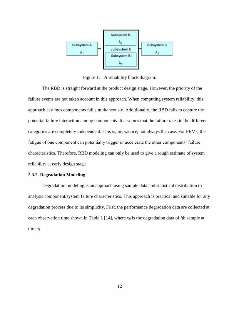
Figure 2 provides an example of a combinatorial block diagram of series and parallel
configurations. The system has Subsystem A, B and C connected in a series configuration.
Subsystem B is formed by Component B1 and Component B2 with being linked in a parallel
configuration. The failure rate of Component B1 and B2 is λ2; Subsystem A and Subsystem C
have failure rates λ1 and λ3 respectively. In this case, the functionality of the system is
demonstrated as Subsystem A and C function with either of B1 or B2 functions. Therefore, the
reliability of the system R is given as:
𝑅 = (1 − 𝜆1)[1 − 𝜆22](1 − 𝜆3) (2)
12
Figure 1. A reliability block diagram.
The RBD is straight forward at the product design stage. However, the priority of the
failure events are not taken account in this approach. When computing system reliability, this
approach assumes components fail simultaneously. Additionally, the RBD fails to capture the
potential failure interaction among components. It assumes that the failure rates in the different
categories are completely independent. This is, in practice, not always the case. For PEMs, the
fatigue of one component can potentially trigger or accelerate the other components’ failure
characteristics. Therefore, RBD modeling can only be used to give a rough estimate of system
reliability at early design stage.
2.3.2. Degradation Modeling
Degradation modeling is an approach using sample data and statistical distribution to
analysis component/system failure characteristics. This approach is practical and suitable for any
degradation process due to its simplicity. Frist, the performance degradation data are collected at
each observation time shown in Table 1 [14], where xij is the degradation data of ith sample at
time tj.

13
Table 1. General Degradation Data Form.
Sample(i) Time(j)
t1 t2 t3 … tm
1 x1,1 x1,2 x1,3 … x1,m
2 x2,1 x2,2 x2,3 … x2,m
3 x3,1 x3,2 x3,3 … x3,m
…
…
…
…
…
…
n xn,1 xn,2 xn,3 xn ,m
Then a distribution is selected to adequately represent the degradation behavior of the
collected data as in Figure 2 [4]. In this example, normal distribution is selected. With the data at
each observation time, the corresponding mean, 𝜇𝑥, and standard deviation, σ𝑥, are estimated at
each observation time. Later, the estimate value of 𝜇𝑥 and σ𝑥 are fitted as a function of time as
𝜇𝑥(𝑡) and σ𝑥(𝑡). This, in general, is done using regression and least square technique.
Figure 2. Degradation distribution pattern.
In the end, the component/system reliability is evaluated. In this example, the calculation
is based on the assumption of normal distribution. Represented as the shaded area in Figure 2,
the probability of failure,𝐹𝐻(𝑥), which is the probability of the failure characteristics falls below
the threshold value, is computed as:
𝐹𝐻(𝑥) = ∫ 𝑓(𝑥, 𝜇𝑥(𝑡), σ𝑥(𝑡))𝑑𝑥𝐻
0 (3)
𝑅𝐻(𝑥) = 1 − 𝐹𝐻(𝑥) (4)
14
where 𝑓(𝑥) is the PDF of normal distribution for degradation process; H is the pre-defined
threshold value; 𝐹𝐻(𝑥) and 𝑅𝐻(𝑥) are the cumulative probability function and the reliability
function respectively.
Systems with high reliability level, like power electronic systems, the failure
characteristic often are positive and gradually ascending over time. In other word, the model
selected must be able to represent the dependency among the components and the positive
increment in the degradation process. According to this attribute, Pan and Balakrishnan [15]
propose to use gamma distribution to capture the increment of failure characteristics data based
on the statistical modeling method. The correlations between these two performance
characteristics is calculated with Birnbaum-Saunders distribution. With the correlation and
marginal reliability distribution, the system level reliability is calculated and the component level
reliability influence the system reliability is determined.
The system level modeling method seems promising in predicting system reliability. The
correlation and the failure characteristics are capture at each measuring time with the degradation
trend monitored. However, this method has the same problem as the RBD approach. It fails in
demonstrating the main elements affecting component lifetime and the failure interaction among
components. Additionally, it requires a huge sample size to obtain sufficient amount of data. If a
sample fails before a measuring time, there may not be enough data available to accurately
estimate the distribution parameters. Furthermore, during the estimating process, the
computation errors may cause the predicted reliability to be inaccurate.
2.3.3. Competing Failure Mode and Related Derivatives
Competing failure modes methodology has been widely accepted in predicting the
reliability of microelectronic devices. It classifies the failure mechanisms into hard (system

15
mechanical) failures and soft (system performance) failures. A hard failure is referring to the
failure makes a system non-functional such as catastrophic failures. A soft failure comes from
the performance degradation of the system, which is slowly losing its ability to accomplish
designated functionalities to a pre-defined unaccepted level. Using a series system configuration,
whichever of the failures comes first, the system fails before other failure modes appear.
Modeling these two types of failures is different as well. A hard failure is normally modeled by a
distribution with time-to-fail data. Meanwhile, the performance data collected over multiple time
point determines the degradation distribution to modeling of a soft failure. Hard failures and soft
failures can be modeled via degradation modeling approach. The system reliability is
demonstrated by the combination of the hard failure distribution and the soft failure distribution.
When the hard failure and the soft failure are independent, the system reliability is the
product of the hard failure relationship and the soft failure relationship. Assuming a system has p
hard failure modes and q soft failure modes. For hard failure, denote the reliability of each hard
failure mode as Rhi(t), for i= 1,2,..., p. Similarly, the reliability of each soft failure mode is
denoted as Rsj(t), for j= 1,2,..., q. Together, the system reliability is calculated as:
𝑅(𝑡) = (∏ 𝑅ℎ𝑖𝑝𝑖=1 (𝑡))(∏ 𝑅𝑞𝑗
𝑞𝑗=1 (𝑡)) (5)
Rafiee et al. [16] propose four models for dependent competing failure processes with
changing degradation rate. A device is undergoing a soft failure process from degradation and
shocks arriving randomly. Additionally, arriving shocks bring a hard failure process. Depending
on how the degradation rate changes after shock arriving, the device reliability is defined as the
product of the soft failure and the hard failure.
The competing failure mode is often used with degradation modeling. Yang and Xue [17]
assume the degradation level follows a standard normal distribution when degradation process is

16
modeled. As the means of standard deviations of the degradation data are estimated at each time
point, the functions of the mean and standard deviation are built. In this case, the reliability of
product can be evaluated by the standard distribution according to the values of the mean and the
standard deviation. Huang and Askin [18] propose the similar method to capture the soft and
hard failures of an electronic device. Assuming degradation process follows Weibull distribution,
the shape parameter, β, and the characteristic life, α, are estimated as functions of time. Thus, the
reliability of the electronic device can be evaluated based on the values of β and α.
The competing failure mode classified the failure modes existing in the system into
different categories and capture the failure characteristic according to their statistical behaviors.
However, as an extension of RDB, competing failure mode assumes the independence
relationship among failure modes or components, which fails to demonstrate the potential failure
interaction among components. Therefore, competing failure mode can only be used as a
complementary approach to RBD at early design stage.
2.4. Bayesian Model Averaging
When using degradation modeling to compute system reliability, there are uncertainties
related to models and parameters values. The principle of Bayesian statistics uses the pre-
determined prior distribution to compute posterior distribution and likelihood function of data.
Based on Bayesian statistics, Bayesian model averaging is a more comprehensive approach to
assess model uncertainty. For a system in which two or more competing failure mechanisms
causing the system break-down, Bayesian model averaging is helpful for addressing the
significant uncertainties among factors which affects the accuracy of posterior distribution for
reliability analysis.

17
Dependent to the data set G, the posterior distribution for the quantity of interest, q, is
given as [19]:
𝑝𝑟(𝑞|𝐺) = ∑ 𝑝𝑟(𝑞|𝑀𝑘 , 𝐺)𝑝𝑟(𝑀𝑘|𝐷)𝐾𝑘=1 (6)
where 𝑀1,…, 𝑀𝑘 are the possible posterior models considered. The posterior probability of
model 𝑀𝑘is
𝑝𝑟(𝑀𝑘|𝐺) =𝑝𝑟(𝑞|𝑀𝑗)𝑝𝑟(𝑀𝑗)
∑ 𝑝𝑟(𝑞|𝑀𝑗)𝑝𝑟(𝑀𝑗)𝐾𝑗=1
(7)
where
𝑝𝑟(𝐺|𝑀𝑘) = ∫ 𝑝𝑟(𝐺|𝜃𝑘 , 𝑀𝑘)𝑝𝑟(𝜃𝑘|𝑀𝑘) 𝑑𝜃𝑘 (8)
is the integrated likelihood of model Mk and 𝜃𝑘 is the vector of parameters of model 𝑀𝑘.
Wang and Gao [20] propose analyzing the system reliability with both insights of failure
mechanisms and understandings of observed data. They use Bayesian model averaging approach
to demonstrate the effect of performance degradation failures, sudden failures and the competing
failure based on the interaction of these two failure modes on the total system reliability level of
complex aircraft engine systems. The performance degradation is assumed follow the Gamma
process. More, to capture the correlation between performance degradation failures and sudden
failures in aspect of the failure mechanism, sudden failures are defined follow the Weibull
distribution where the shape parameter is characterized the performance degradation. The
competing failure is defined as the joint distribution of the performance degradation and sudden
failure. Applying Bayesian forecast probability density function, the total system reliability of
complex aircraft engine systems, which is given the reliability of performance degradation
failures, sudden failures and the competing failure, is calculated with consideration of data
correlation and failure mechanism.

18
The Bayesian average modeling provides an effective way of combining prior
information with data and inferences that conditional on the data to evaluate system reliability.
However, it is difficult to select a prior distribution for the assumption of unknown parameters.
In practice, due to the limited knowledge, a prior distribution cannot be specified. Further,
Bayesian average modeling has a high computational cost, especially when the model has a large
number of parameters. In many cases, the integrals are not feasible to compute. Therefore,
Bayesian average modeling does not have a wide application.
2.5. Physics of Failure Modeling
Physics-of-Failure (PoF) model is an approach that assesses component lifetime and
predicts component reliability through utilizing the knowledge of product’s failure mechanisms
at different life-cycle loading conditions [21]. Understanding the PoF model of power electronic
modules helps researchers capture the failure characteristics and performance behaviors of power
electronic modules over time. Over the past decades, two major failure mechanisms of power
electronic modules: wire bond lift-off and solder joint delamination, have been observed and
identified. Therefore, the corresponding PoF models have been modeled and developed.
2.5.1. Wire Bond Lift-off
The IGBT break-down occurs most of the time due to wire bond lift-off. Aluminum wire
bonds are soldered onto silicon chips to connect the emitter and gate pads. The sandwich
structure of power electronic module consists of different types of materials. In this case,
aluminum wire and silicon chips are heterogeneous materials and soldered together. When
IGBTs are loaded and functioning, they undergo temperature amplitude. Due to the large
coefficient of thermal expansion (CTE) difference, aluminum out expanse silicon and cracks

19
start to form and propagate in the wire bonds. The thermal model of the Al-Si interface heating
up is shown in Figure 3 [22].
Figure 3. The thermal model of the Al-Si interface heating up.
Onuki and Koizumi [23] use transmission electron microscope (TEM) and scanning
electron microscope (SEM) to investigate the microstructures of the bonding interface.
Theoretically, the crack should have formed and propagated along the weakest area, which is the
interconnected area of the Al-Si interface. But they found out that the crack travels along the
grain boundary between the interface of Al-Si interface and Aluminum wire coincidently. Due to
the small grain size the interface has, it becomes the boundaries for cracks later. This explains
the reason crack doesn’t propagate along the Al-Si interface.
Geohre et al. [22] monitor the crack propagation process in the Aluminum and Silicon
interface. They found out that the crack is propagating 10-20 μm above the interface as shown in
Figure 4. Ramminger et al.[24] study the SEM photograph of the bonding area after wire bond
lifts off. The residual material of Aluminum wire is found on the pattern perimeter instead of the
middle of the bonding area. It can be concluded that cracks initiate from the both end of the wire
bond to the center. The mismatch of the coefficients of thermal expansion of the materials at the
bonding interface leads to large plastic strains. These plastic strains drive the propagation of
micro cracks leading to the fatigue failure of wire bond.

20
Figure 4. Crack propagates above the interface of Al-Si film.
Schafft [5] claims that smaller grains are formed, compared to Aluminum wires, in the
Al-Si film by metal’s re-crystallization effect during the soldering process. Therefore, grain
boundaries are formed between the interface and Aluminum wires due to different grain size.
According to material properties, metals with smaller grain size have greater material strength
and toughness. As shown in Figure 5 [23], the bonding interface and Al-Si film have a smaller
grain size compared to the wire, which indicates higher material strength in the bonding interface
and Al-Si film. When thermal stress is induced, these two sections can stand the shear and tensile
force better than the wire. Hence, cracks start initiating and propagating along the grain boundary.
Figure 5. Wire bond interface after fatigue.
From the findings about wire bond fatigue phenomena, it can be concluded that
Aluminum wire is vulnerable under the wire bond fatigue process. Therefore, PoF models have
been developed to seize and describe the physical dimensional change of wire. Schafft [5]

21
measures the geometry change of the height of the wire loop to study the thermal fatigue induced
by flexing. The model is sketched in Figure 6. The change of the height of the wire loop is given
as:
ℎ = ℎ𝑜 [1 +1
8(7 +
3
2
𝑑02
ℎ𝑜2 ) × 𝐶𝑇𝐸𝑤 × ∆𝑇] (9)
where h0 is the original height of the wire loop; CTEw is the CTE of Aluminum wire; n
represents the ratio of the wire length at the original temperature to the time that the bond is
separate; d0 is defined as the length of the wire bond span; ∆𝑇is the amplitude of temperature
swing.
Figure 6. Geometry change of model of wire bond.
Schafft[2] also study the change of the angle of wire loop. Depending on the type of wire
connections, two models have been proposed. For Angular shaped loop,
cos 𝜑 = cos 𝜑𝑜 (1 − ∆𝐶𝑇𝐸 × ∆𝑇) (10)
For a circular arc shaped loop
sin 𝜑
𝜑=
sin 𝜑𝑜
𝜑𝑜(1 − ∆𝐶𝑇𝐸 × ∆𝑇) (11)
where𝜑𝑜is the original angle of the wire loop; ∆𝐶𝑇𝐸is the difference of CTEs between
Aluminum and Silicon; ∆𝑇 is the amplitude of temperature swing.
During the thermal fatigue process, the material properties of Aluminum wire and Silicon
chip change depend on the temperature amplitude. Schafft [5] monitors the main material

22
properties, including CTEs of Aluminum and Silicon and the elastic-plastic material law of
Aluminum. Table 1 and Table 2 [5] show that the material properties of wires and silicon chip at
various temperatures.
Table 2. CTEs of Wires and Chips at Various Temperatures.
Al Cu Mo Si
200K 2.15E-05 1.59E-05 4.80E-06 1.90E-06
300K 2.32E-05 1.68E-05 5.00E-06 2.50E-06
400K 2.49E-05 1.77E-05 5.20E-06 3.10E-06
500K 2.64E-05 1.83E-05 5.30E-06 3.50E-06
Table 3. Elastic-plastic Change of Aluminum at Various Temperatures.
20°C 60°C 100°C
σy [MPa] 26.9597 20.6194 19.1296
ϵy [%] 0.29 0.37 0.38
A [MPa] 53.4067 45.1201 40.9685
B [1] 0.125738 0.126055 0.125146
ϵo [%] 0.4354 .20046 0.22758
Geohre et al.[22]estimate the plastic strains per cycle in the Al by assuming Al and Si
undergo the equal strain with Si only having elastic material behavior and Al only having ideal
plastic material behavior. According to Figure 3, Geohre et al. [22] model the plastic strength of
Aluminum wire given as:
∆𝜀𝑝𝑙𝐴𝑙 = ∆𝐶𝑇𝐸∆𝑇 − 2 (
𝜎𝑦𝐴𝑙
𝐸𝑆𝑖 +𝜎𝑦
𝐴𝑙
𝐸𝐴𝑙) (12)
where ∆𝜀𝑝𝑙𝐴𝑙is the plastic strain on Aluminum wire; ∆𝐶𝑇𝐸is the different of material CTE; ∆𝑇is
temperature amplitude; 𝜎𝑦𝐴𝑙is the tensile force induced on the Aluminum wire by thermal fatigue
process; 𝐸𝑆𝑖and 𝐸𝐴𝑙 are the elastic indices for Silicon and Aluminum respectively. From the
Table 2, the value of 𝜎𝑦𝐴𝑙 decreases as temperature amplitude increases. Therefore, the value of
∆𝜀𝑝𝑙𝐴𝑙 becomes larger as temperature amplitude increases in the equation above, which
demonstrating faster fatigue failure of wire bond when temperature amplitude is high.

23
Another approach to test the wire bond lift-off is shear force test [5]. A horizontal force is
applied by a probe to test the adhesive force of the wire bond. The degree of the bond adhesive is
measured corresponding to the force which breaches the wire bond [5]. The problem of the
approach is the difficulty of designing a probe that is small enough to stand the applied force and
breach the wire bond. Moreover, the operator's reproducibility is also another major concern [5].
Through experiment data and measurement, Geohre et al. [22] reveal, illustrated in
Figure 7, the shear force of the bonding area (sheared area) between Si chip and Al wire
decreases as the bonding area (sheared area) shrinks as the degradation process deteriorates.
Figure 7. Shear force v.s. sheared area.
Thus, the bond degradation process can be quantified with shear force as a parameter.
From Figure 7, it is clear that the shear force decreases as sheared area decreases due to crack
growth and reduction of the wire bonding area [25]. The shear force at different crack length is
given as:
𝐹𝑠 = (𝐿−𝑙
𝐿) 𝐹0 (13)
where l is the crack length in the bonding area; L is the initial bond length; F0 is the initial shear
force existing in the wire bonding area; Fs is the remaining shear force after n cycles.

24
In order to capture the wire bond fatigue failure process, the component lifetime is linked
to the variables contributing to component fatigue failure. Geohre et al. [22] measure the
relationship between average shear force and number of cycles to failure in different temperature
amplitude. It reveals that larger temperature amplitude results in lower number of cycles to
failure. The same phenomenon is observed with average sheared area and number of cycles. It
can be concluded that when crack propagates, the bonding force of Aluminum wire and Silicon
chip decreases as the wire bonding area is detaching. Based on the observation, Geohre et al.
[22] propose to use Coffin-Mason relationship to capture number of cycles to failure with the
parameter of the calculated plastic strains. The equation is given as:
𝑁𝑓 = 0.309(∆𝜀𝑝𝑙𝐴𝑙)−1.764 (14)
where 𝑁𝑓 is the number of cycles to fail and ∆𝜀𝑝𝑙𝐴𝑙 is the plastic strains on wire bond.
Held et al.[6] report that the temperature amplitude and the median temperature are the
significant factors affecting IGBT's lifetime. Taking plastic deformation and material properties
into account, the model they proposed, which integrates Arrhenius approach and indicates a
linear relationship.
𝑁𝑓 = 𝐴∆𝑇𝛼𝑒𝑥𝑝 (𝑄
𝑅𝑇𝑚) (15)
where ∆T is the temperature amplitude in Kelvin, A= 640, α= -5, Q= 7.8×10⁴ J/mol, R is the gas
constant, which is 8.314 J/(mol∙K), and Tm is the median temperature in Kelvin. Taking double
logarithm of the equation, this model provides a straight line relationship, shown in Figure 8, to
determine the number of cycles to failure with the temperature amplitude and the median
temperature as parameters.

25
Figure 8. Number of cycles to failure v.s. ∆T and Tm.
2.5.2. Solder Joint Delamination
Solder joint is another critical component affecting IGBT system reliability. A solder
joint is a component joint soldering silicon chips to the substrate and provides electrical, thermal
and mechanical continuity to IGBT module. A solder joint consists with different materials
depending the choices of materials, such as lead-based (SnPb) or lead-free (SnAgCu) solders.
Made of different alloys, solder joint has an inhomogeneous structure [26]. Due to the thermo-
mechanical stress, the grain size of solder layer grows over the elevated temperature leading to
the reduction of internal energy of solder structure and the weakening of the grain boundaries
[26]. Thus, voids are resulted inducing cracks propagate in solder joint. This accumulative
fatigue phenomenon is illustrated in Figure 9.
Figure 9. Accumulative fatigue phenomenon of solder joint.

26
To quantify the relationship between number of cycles to failure and the material damage
caused by the thermal fatigue, lifetime prediction models have been developed. The most
classical model is Coffin-Manson model taking into account the material damage caused by
plastic strain range given the component lifetime as [27]:
𝑁𝑓 =1
2(
∆𝛾𝑝
2𝜀𝑓)
1/𝑐
(16)
where 𝜀𝑓 is the fatigue ductility coefficient and c is the fatigue ductility exponent depending
material property; ∆𝛾𝑝 is the plastic strain range.
On the basis of Coffin-Manson model, Solomon model [28] considers the shear plastic
strain as the main cause of solder joint fatigue. The solder joint lifetime is given as:
∆𝛾𝑝𝑁𝑓𝛼 = 𝜃 (17)
where 𝜃 is the reciprocal of fatigue ductility coefficient while α is the material constant.
The root cause of thermal-mechanical stress is temperature amplitude applied to IGBT
module. Higher temperature amplitude results in strong stress in solder joint and, therefore,
shorter component lifetime. Choi et al [29] use Coffin-Manson model to explain this fatigue
failure process and the solder joint lifetime is given as:
𝑁𝑓 = (𝑝
∆𝑇)
𝑘
(18)
where p and k are the material constants dependent to selected solder materials; ΔT is the
temperature amplitude.
Yin et al [30] propose a strain based lifetime prediction model given as:
𝑁𝑙 =𝑙
𝑞(∆𝜀𝑝)𝑔 (19)
where l is the crack length solder joint; ∆𝜀𝑝 is the plastic strain while Nl is the corresponding
number of cycles until crack reaches the length l.

27
Mitic et al. [31] test the adhesion force between AlN ceramic substrates and their solder
joints with a peel test. The largest decrease in the adhesion force happens after 80 thermal cycles.
Hung et al. [32] investigate the impact of solder height on fatigue life of IGBT. The scanning
acoustic microscope results indicate the solder crack length propagates from the corners of
substrate towards the center as shown in Figure 10. However, the solders in high solder height
show slower crack growth rate. Some thick solders show no crack found in the module after
thermal cycling. Figure 7 shows the crack lengths of different solder height after 450 thermal
cycles. When the solder height gets beyond 300 um, no significant crack is found. This is
because increasing the thickness of solder joint restrains solder joint structure deformation [32].
Figure 10. Crack lengths of different solder heights after 450 thermal cycles.
To quantify the impact that the physical dimension of solder joint has on component
lifetime prediction, Ciappa [33] proposes an equation to capture the relationship between solder
joint’s number of cycles to failure and temperature swing.
𝑁𝑓 = 0.5(𝐿∆𝐶𝑇𝐸∆𝑇
𝛾𝑥)1/𝑐 (20)

28
where ΔCTE represents the CTE mismatch, 𝛾 and 𝑥 are the ductility factor and the thickness of
the solder, and L is the lateral size of the solder joint. 𝛾 and c are conservative engineering
estimates dependent to materials chosen.
Recently, Advani and Yadav [8] studies the crack propagation process in solder joint. He
classifies the process into two phases: crack initiation and crack propagation. Unlike the
traditional approach, which monitors the change of grain size in solder alloy to determine the
crack initiation, Gurmukh proposes to use the resistance of solder alloy as an indicator. Once a
threshold value is reached, the solder joint is in its crack propagation phase. With Cubic
Coarsening model and Coffin-Mason model proposed for each phase respectively, the all over
system reliability model of solder joint is the combination of these two phases. With proper
statistical assumptions for different phases, Advani and Yadav [20] evaluates the reliability
model according to either the failure distribution over time or the damage accumulation on the
quality characteristics.
The physics of failure model approach links the physics properties and component
lifetime in depth. However, it only concentrates on one particular component's failure
mechanism. Also, the correlation between components, in this case, the failure interaction
between wire bond and solder joint is ignored. Additionally, the lack of probabilistic modeling
makes PoF modeling fail in demonstrating the system reliability. In addition, the failure
interaction between solder joint and wire bond has been studied with literature pointing out that
wire bond lift-off is dominant failure mechanism. Therefore, the solder joint degradation process
is triggered by wire bond lift-off phenomenon in this work.
29
3. PROPOSED RELIABILITY MODEL
In this section, a new system reliability model is proposed overcoming the disadvantages
or research gap mentioned in literature review section. First, the proposed model uses selected
PoF models to present the failure mechanism of critical components. Second, probabilistic
interpretation is provided based on the PoF models. Third, system reliability is calculated in a
series configuration and the failure mechanism interaction is considered. The cumulative effect
of the degradation of wire bond and solder joint is updated to take account for system reliability
at each cycle. Additionally, the system reliability model is classified into two phases considering
the predominant of wire bond degradation process over solder joint.
3.1. Initial PoF Models Selection
The PoF models for wire bond lift-off and solder joint delamination are reviewed in the
previous section. In this subsection, certain PoF models are selected to present and model the
failure mechanism of wire bond or solder joint. Critical factors affecting component lifetime,
such as temperature amplitude and physical dimensions, are demonstrated comprehensively in
these models to provide accurate estimates on component lifetime. The selected models for wire
bond and solder joint are discussed in the following sections.
3.1.1. Solder Joint PoF Model
Solder joint delamination is caused by the thermo-mechanical strain induced by the
temperature amplitude. As discussed in the literature review section, the thermo-mechanical
strain becomes larger when the temperature amplitude increases. Moreover, as Micol et al [7]
pointed out, the initiation of solder joint failure characteristics is closely related to the geometric
shape of the solder joint. Cracks propagates slower in a smaller growth rate in thick solder joint
due to the deformation process is restricted [33] and the lateral size of the solder layer has a

30
direct impact on the magnitude of shear strain generated in solder layer. Additionally,
manufactured with different alloy materials, the solder joints lifetime varies. The main categories
are Pb-based solders and Pb-free solders. [34] have proven that Pb-free solders have better
reliability due to high yield strength and cracks are not dependent to plastic deformation in the
solder microstructure. Therefore, the model from [33] is selected to estimate the solder joint
lifetime:
𝑁𝑓𝑠 = 0.5(𝐿∆𝐶𝑇𝐸∆𝑇
𝛾𝑥)1/𝑐 (21)
where ΔT is the temperature amplitude of power cycling, ΔCTE is the difference of the CTEs
among Solder layer materials, x is the thickness of the solder, and L is the lateral size of the
solder joint; γ, which is the ductility factor, and c are conservative engineering estimates
depending on materials chosen.
The reason that Equation (21) is selected is because the solder joint lifetime is predicted
based on the design and operational conditions as discussed earlier. Critical physical dimensions
such as thickness and lateral size of different solder materials are considered, such as x, L, c and
γ in the equation. Thermo-mechanical strain is also captured dependent on the operational
conditions, mainly temperature amplitude, ∆𝑇. Therefore, from Equation (21), solder joint
lifetime is demonstrated comprehensively.
3.1.2. Wire Bond PoF Model
The wire bond has the same cause for failure mechanism as the solder joint. The
mismatch of material CTEs induces thermo-mechanical stress in wire bond when temperature
amplitude is enforced. The magnitude of thermo-mechanical stress is determined by the
temperature amplitude applied to the module. This relationship is often demonstrated by power
law [10][22] and, therefore, temperature amplitude is the important factor account for wire bond

31
degradation process. Additionally, Held et al [6] test the wire bond lifetime in the same
temperature amplitude but with different mean temperatures. A parallel shift is observed for
different mean temperatures when the degradation data is plotted in Arrhenius model [6].
Therefore, based on these findings, the wire bond lifetime model is given as:
𝑁𝑓𝑤 = 𝐴∆𝑇𝛼𝑒𝑥𝑝𝑄
𝑅𝑇𝑚 (22)
where ∆T is the temperature amplitude in Kelvin, A= 640, α= -5, Q= 7.8×10⁴ J/mol, R is the gas
constant, which is 8.314 J/(mol∙K), and Tm is the median temperature in Kelvin.
Compared to most of the PoF models in other literatures [22][35][36], which mainly
focus on the relationship between shear strain and numbers of cycles, Equation (22) details the
wire bond lifetime not only with the effect from temperature amplitude, but also the parallel shift
of wire bond lifetime trend from different mean temperatures due to various operational
conditions as found in [6]. Therefore, the solder joint lifetime is represented comprehensively via
Equation (22).
3.2. Probabilistic Modeling
From Equation (21) and (22), the number of cycles to failure for solder joint and wire
bond can be easily estimated. However, in practice, the fatigue damage is of stochastic nature
due to the randomness in material fatigue behavior and loading conditions [37]. In order to
provide more realistic estimate of system reliability, it is, therefore, necessary to convert
deterministic modeling into probabilistic modeling. The following sections provide detailed
discussion on probabilistic modeling.
First, component lifetime is closely related to temperature amplitude applied to PEM
modules. Higher temperature amplitude results in shorter component lifetime. Treating
temperature amplitude as the stress, it is reasonable to use the S-N curve to demonstrate the
32
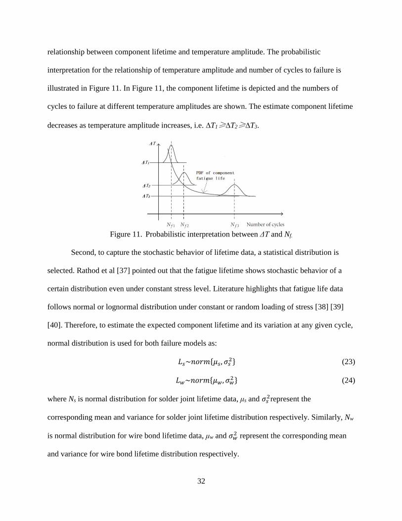
relationship between component lifetime and temperature amplitude. The probabilistic
interpretation for the relationship of temperature amplitude and number of cycles to failure is
illustrated in Figure 11. In Figure 11, the component lifetime is depicted and the numbers of
cycles to failure at different temperature amplitudes are shown. The estimate component lifetime
decreases as temperature amplitude increases, i.e. ∆T1≥∆T2≥∆T3.
Figure 11. Probabilistic interpretation between ΔT and Nf.
Second, to capture the stochastic behavior of lifetime data, a statistical distribution is
selected. Rathod et al [37] pointed out that the fatigue lifetime shows stochastic behavior of a
certain distribution even under constant stress level. Literature highlights that fatigue life data
follows normal or lognormal distribution under constant or random loading of stress [38] [39]
[40]. Therefore, to estimate the expected component lifetime and its variation at any given cycle,
normal distribution is used for both failure models as:
𝐿𝑠~𝑛𝑜𝑟𝑚{𝜇𝑠, 𝜎𝑠2} (23)
𝐿𝑤~𝑛𝑜𝑟𝑚{𝜇𝑤, 𝜎𝑤2 } (24)
where Ns is normal distribution for solder joint lifetime data, μs and 𝜎𝑠2represent the
corresponding mean and variance for solder joint lifetime distribution respectively. Similarly, Nw
is normal distribution for wire bond lifetime data, μw and 𝜎𝑤2 represent the corresponding mean
and variance for wire bond lifetime distribution respectively.
33
Additionally, components tend to fail in a short time span if the applied stress level, ΔT,
is high. The phenomena is observed as the spread of the distribution increases as component
lifetime increases and temperature amplitude decreases. Therefore, it is reasonable to assume the
variance is proportion to the estimate lifetime. From the above rationale, the probability density
function of component lifetime for both models at any specific cycle, N, are given as:
𝑓𝑤(𝑁) =1
𝜎𝑁𝑓𝑤√2𝜋
𝑒𝑥𝑝 (−1
2(
𝑁−𝑁𝑓𝑤
𝜎𝑁𝑓𝑤
)
2
) =1
𝜎𝑁𝑓𝑤√2𝜋
𝑒𝑥𝑝 (−1
2(
𝑁−𝑁𝑓𝑤
𝑚𝑤×𝑁𝑓𝑤)
2
) (25)
𝑓𝑠(𝑁) =1
𝜎𝑁𝑓𝑠√2𝜋
𝑒𝑥𝑝 (−1
2(
𝑁−𝑁𝑓𝑠
𝜎𝑁𝑓𝑠
)
2
) =1
𝜎𝑁𝑓𝑠√2𝜋
𝑒𝑥𝑝 (−1
2(
𝑁−𝑁𝑓𝑠
𝑚𝑠×𝑁𝑓𝑠)
2
) (26)
where mw and ms the proportion coefficients for wire bond and solder joints.
3.3. Modeling Component Failure Mechanism Interaction
In the previous section, PDF of fatigue life for each component is defined and
established. However, to provide more realistic estimate to model system reliability, the lifetime
model needs to take account for the failure mechanism interaction between wire bond and solder
joint degradation process. In this particular work, the increase in junction temperature caused by
initiation of one failure or degradation process and its impact of other degradation processes have
been investigated.
For wire bond lifting off phenomenon, one wire lifting off the bonding area will cause
increases in the current load on the remaining wires. This phenomenon worsens the self-heating
in the remaining wires and causes higher junction temperature in bonding area. The changes in
junction temperature induced by the degradation process of wire bond with different bonding
techniques is shown in Figure 12 [41].

34
Figure 12. Junction temperature values versus the number of cycles.
The wire bond lift-off is accelerated due to the increased junction temperature. Cracks
propagate towards the center of the bond foot until the wire completely lifts off from the bonding
area causing the termination of the mechanical and electrical contact of the metallization.
Moreover, increase in junction temperature results in increase in collector-emitter voltage
(VCE) [42] and, therefore, VCE is used as an indicator for wire lifting. Gradual increase in VCE has
been detected, shown in Figure 13, regardless to wire bonding techniques during power cycling
process [41]. Additionally, the literature shows majority of the tested modules failed due to wire
bond lift-off phenomenon [47]. From the above observation, it is concluded that wire bond lift-
off is the predominant failure mechanism for IGBT modules when temperature amplitude is
under 130 K [34] [42] [44].
35
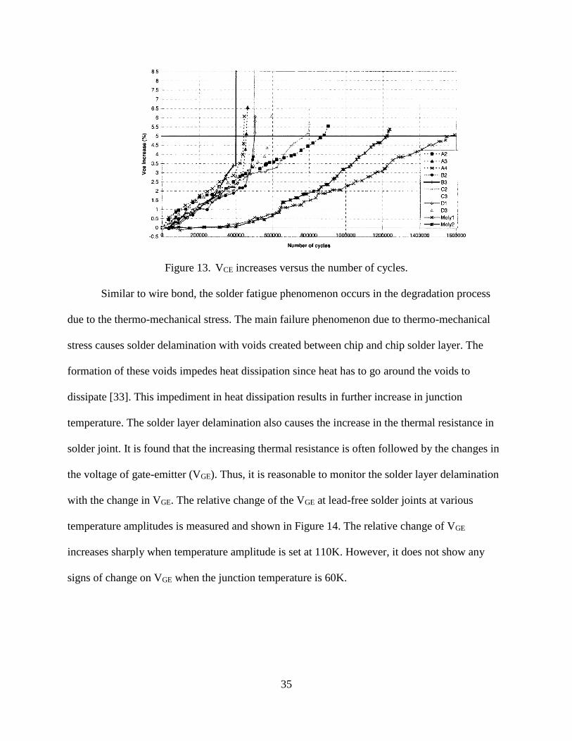
Figure 13. VCE increases versus the number of cycles.
Similar to wire bond, the solder fatigue phenomenon occurs in the degradation process
due to the thermo-mechanical stress. The main failure phenomenon due to thermo-mechanical
stress causes solder delamination with voids created between chip and chip solder layer. The
formation of these voids impedes heat dissipation since heat has to go around the voids to
dissipate [33]. This impediment in heat dissipation results in further increase in junction
temperature. The solder layer delamination also causes the increase in the thermal resistance in
solder joint. It is found that the increasing thermal resistance is often followed by the changes in
the voltage of gate-emitter (VGE). Thus, it is reasonable to monitor the solder layer delamination
with the change in VGE. The relative change of the VGE at lead-free solder joints at various
temperature amplitudes is measured and shown in Figure 14. The relative change of VGE
increases sharply when temperature amplitude is set at 110K. However, it does not show any
signs of change on VGE when the junction temperature is 60K.

36
Figure 14. Relative change of VGE versus the number of cycles.
Based on the observation above and combined with the wire bond failure process, the
behavior of solder joint degradation is further detailed according to the change of VGE depicted
in Figure 15. The relative change of VGE remains constant at the beginning of the power cycling
test since no sign of solder degradation shown. However, as wire bond lift-off is the predominant
failure mechanism, junction temperature rises slowly due to the self-heating phenomenon of
wires as the wire bond fatigue continues. When junction temperature increases to a certain
magnitude, cracks are initiated in solder joint causing changes in VGE. As illustrated in Figure 15,
the crack initiation phase ends at NSI cycles and crack propagation phase starts. Therefore, the
change in VGE value can be used as a measure to decide when solder joint degradation is
triggered. The subsequent increase in junction temperature can be attributed to the cumulative
effect of the degradation process of wire bond and solder joint.

37
Figure 15. Change of ΔVGE in solder joint.
From the reasoning above, the junction temperature increases at faster rate once the
degradation of solder joint starts. Simultaneously, the degradation process of solder joint and
wire bond is accelerated by the increasing junction temperature. Therefore, the failure interaction
between wire bond and solder joint occurs through the increasing junction temperature.
Therefore, capturing the increasing junction temperature becomes the focal point of this work to
model failure interaction and provide realistic system reliability prediction. This process is
detailed as follows.
Considering only wire bond and solder joint IGBT subjected to degradation process and
the predominance of wire bond degradation process over solder joint, it is reasonable to consider
that failure mechanism of wire bond starts first in most of cases. Therefore, the initial increase in
junction temperature is resulted from the wire bond failure process. The junction temperature is
given as:
∆𝑇′ = ∆𝑇 + ∆𝑇𝑗𝑤 (27)
where ∆𝑇 is original temperature amplitude and ∆𝑇𝑗𝑤 is the amount of increase in junction
temperature caused by wire bond.

38
Once the cracks start at NSIth cycle, crack propagation leads to solder joint fatigue and
junction temperature is raised resulting from the cumulative effect of both wire bond and solder
joint fatigue. Therefore, the increase in junction temperature after NSIth cycle is given as:
∆𝑇′ = ∆𝑇 + ∆𝑇𝑗𝑠 + ∆𝑇𝑗𝑤 (28)
where ∆𝑇 is original temperature amplitude; ∆𝑇𝑗𝑤 is the amount of increase in junction
temperature caused by wire bond while ∆𝑇𝑗𝑠 is the amount of increase in junction temperature
caused by solder joint.
The heat generated by the rising junction temperature due to component degradation can
be determined via Joule’s Law with component failure indicators. For the purpose of simplicity,
we assume that there is no heat loss. According to First Law of Thermodynamics, the heat
generated by the rising junction temperature by wire bond or solder joint can be given as:
∆𝑄𝑠 =∆𝑉𝐺𝐸
2𝑁
𝐼= 𝐶𝑠𝑚𝑠∆𝑇𝑗𝑠 (29)
∆𝑄𝑤 =∆𝑉𝐶𝐸
2𝑁
𝐼= 𝐶𝑤𝑚𝑤∆𝑇𝑗𝑤 (30)
where N is the number of cycles; I is the current applied on the module; Cs and Cw are the
specific heat capacity of component solder joint and wire bond; ms and mw are the mass of solder
joint and wire bond; ∆𝑇𝑗𝑠 and ∆𝑇𝑗𝑤 are the amount of the temperature raised by solder joint and
wire bond respectively.
Thus, the rising junction temperature induced by the degradation process of solder joint
and wire bond at any given cycle are given as:
∆𝑇𝑗𝑠 =∆𝑉𝐺𝐸
2𝑁
𝐼𝐶𝑠𝑚𝑠 (31)

39
∆𝑇𝑗𝑤 =∆𝑉𝐶𝐸
2 𝑁
𝐼𝐶𝑤𝑚𝑤 (32)
To obtain the value of VGE and VCE at the corresponding cycle, the statistical behavior of
VGE and VCE is studied. From Figure 14 and Figure 15, VGE and VCE monotonically increase as
the power cycling continues. Through the result of empirical degradation model, the failure
characteristics of degradation process grows exponentially as a function of time and therefore,
exponential distribution provides a good fit to capture the behavior of the increased thermal
resistance as shown in Figure 16 [45]. Therefore, it is reasonable to model the behavior of VGE
and VCE with exponential fit.
Figure 16. Behavior of thermal resistance.
With the increased junction temperature being calculated through Equation (31) and (32)
at any given cycle, the effect of failure mechanism interaction is incorporated with the expected
lifetime of wire bond and solder joint modified. The modified equations for the expected lifetime
of solder joint and wire bond are given as:
𝑁𝑓𝑠′ = 0.5(
𝐿∆𝐶𝑇𝐸∆𝑇′
𝛾𝑥)1/𝑐 (32)
𝑁𝑓𝑤′ = 𝐴∆𝑇′𝛼𝑒𝑥𝑝 (
𝑄
𝑅𝑇𝑚) (33)
40
where 𝑁𝑓𝑠′ and 𝑁𝑓𝑤
′ are the number of cycles to failure for solder joint and wire bond respectively
with the updated junction temperature; the rest of the remaining terms are the same as defined in
Equation (21)(22).
The probabilistic model is updated with the increase junction temperature is given as:
𝐿′𝑠(𝑁)~𝑛{𝜇′𝑠(𝑁), 𝜎′𝑠2(𝑁)} (35)
𝐿′𝑤(𝑁)~𝑛{𝜇′𝑤(𝑁), 𝜎′𝑤2 (𝑁)} (36)
3.4. System Reliability Modeling
The system reliability is computed based on a series configuration since either of wire
bond or solder joint fails will results in the break-down of IGBT module. In general, the system
reliability for series configuration is calculated as the product of the reliability of each individual
component as given below:
𝑅(𝑁) = 𝑅1(𝑁) × 𝑅2(𝑁) × ⋯ × 𝑅𝑘(𝑁) (37)
where k is the total number of components in system.
In this work, only wire bond and solder joint are considered as critical failure
mechanisms causing the degradation process of IGBT module. Therefore, Equation (37) is
modified as:
𝑅(𝑁) = 𝑅′𝑠(𝑁) × 𝑅′𝑤(𝑁) (38)
where 𝑅𝑠(𝑁) is the reliability of solder joint at Nth cycle and 𝑅𝑤(𝑁) is the reliability of wire
bond.
However, reliability prediction for IGBT module based on Equation (38) is not realistic
because it assumes independence relationship between solder joint and wire bond and ignore the
interaction among failure mechanisms. The failure mechanism interaction is demonstrated as one
component’s fatigue failure can trigger or accelerate other component’s failure mechanism

41
through increased junction temperature. Therefore, to demonstrate the effect of failure
mechanism interaction, system reliability is computed in two phases according to Section 3.3.
In the first phase, before NSIth cycle, wire bond lift-off is the predominant failure
mechanism in IGBT module because solder joint does not show any sign of degradation. Thus,
the product lifetime is solely depending on the performance of wire bond. The increases in
junction temperature is attributed to the fatigue failure of wire bond lift-off and the failure
characteristics is affected by the updated junction temperature at any given cycle.
At each cycle N, the increases in junction temperature attributed by degradation process
of wire bond can be computed through Equation (29) and the overall junction temperature is
given by Equation (27). With the overall junction temperature, the estimate component lifetime
is computed via Equation (34) and the probabilistic distribution of wire bond lifetime is updated.
Therefore, the system reliability is the probability that the IGBT module can survives beyond the
expected lifetime cycle of wire bond at the current cycle:
𝑅𝑠𝑦𝑠𝑡𝑒𝑚 = 𝑅′𝑤(𝑁 > 𝑁𝑤′ ) (39)
Second phase, starting from NSIth cycle, due to the increased junction temperature
induced by wire bond degradation, solder joint degradation process is triggered and accelerated.
Meanwhile, solder joint degradation process affects junction temperature and accelerates the
propagation of crack in wire bond failure process. Thus, the degradation process of both
components are accelerated and system reliability is reduced tremendously.
Similarly to the first phase, the increase junction temperature caused by degradation
process of wire and solder joint is captured by Equation (29) and (30). Thereafter, overall
junction temperature can be computed via Equation (28). The probabilistic distribution for wire
bond and solder joint is updated once the overall junction temperature is obtained. Therefore, the

42
system reliability is the product of the probability that the IGBT module can survives beyond the
expected lifetime cycle of each component at the current cycle:
𝑅𝑠𝑦𝑠𝑡𝑒𝑚 = 𝑅′𝑤(𝑁 > 𝑁𝑤′ ) × 𝑅′𝑠(𝑁 > 𝑁𝑠
′) (40)
Therefore, dependent to the above reasoning, the system reliability is computed in two
situations and the NSIth cycle is the critical value for the prediction process. The combine model
is provided as follows.
SIssww
SIwW
NNforNNRNNR
NNforNNRT
)()(
)({'
''''
''
(41)

43
4. EXAMPLE
In this section, a numerical example is provided to demonstrate the applicability and
effectiveness of the proposed reliability approach.
4.1. Background
An IGBT module has an inhomogeneous structure consisting of different components
with various CTEs. The free expansion of component materials is restricted as they are bonded
together. The temperature amplitude IGBT module undergoes while functioning leads to the
degradation of the module. Due to the larger mismatch of CTEs, thermo-mechanical stress is
generated and occurs in the solder joint and wire bonding area when the temperature amplitude
induces. Since interconnected, the restriction or limitations on the thermal expansion of material
leads to initiation of cracks causing degradation in solder joint and wire bonding area. The
mechanical and electrical connections among components are terminated once cracks slowly
propagate to a critical length separating the component from the module in wire bonding area
and solder joint layer and marking the failure of the module.
As evident from Equation (21) and (22), the expected lifetime of component wire bond
and solder joint can be estimated once the temperature range of power cycling and the physical
dimensions of components are decided. However, due to the interaction among failure
mechanisms during the degradation process, the component expected lifetime gets reduced. The
example is based on the failure behavior of IGBT module during power cycling. Solder joint and
wire bond go through a thermal fatigue process accompanied with cracks initiated and propagate
in these components. As mentioned in previous section, the inspection for the failure behaviors
of solder joint and wire bonding area can be executed by monitoring the increase pattern of VGE
and VCE due to the proportional relationship between the pattern and the failure behavior. Once
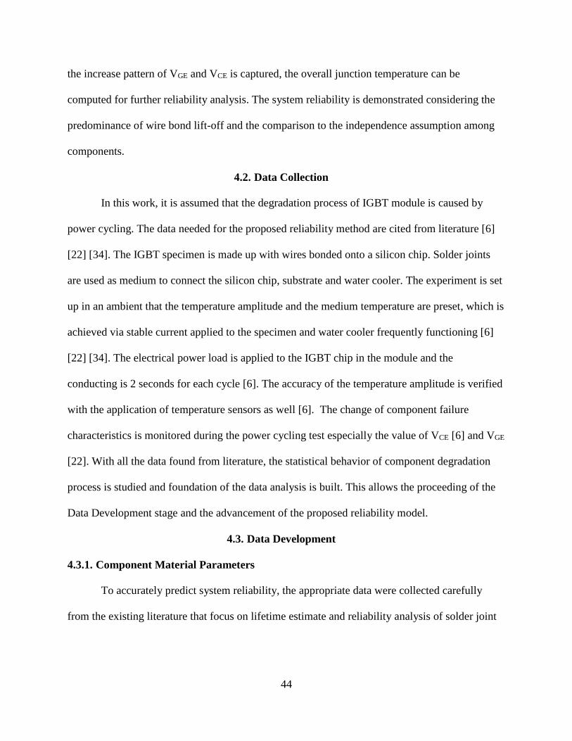
44
the increase pattern of VGE and VCE is captured, the overall junction temperature can be
computed for further reliability analysis. The system reliability is demonstrated considering the
predominance of wire bond lift-off and the comparison to the independence assumption among
components.
4.2. Data Collection
In this work, it is assumed that the degradation process of IGBT module is caused by
power cycling. The data needed for the proposed reliability method are cited from literature [6]
[22] [34]. The IGBT specimen is made up with wires bonded onto a silicon chip. Solder joints
are used as medium to connect the silicon chip, substrate and water cooler. The experiment is set
up in an ambient that the temperature amplitude and the medium temperature are preset, which is
achieved via stable current applied to the specimen and water cooler frequently functioning [6]
[22] [34]. The electrical power load is applied to the IGBT chip in the module and the
conducting is 2 seconds for each cycle [6]. The accuracy of the temperature amplitude is verified
with the application of temperature sensors as well [6]. The change of component failure
characteristics is monitored during the power cycling test especially the value of VCE [6] and VGE
[22]. With all the data found from literature, the statistical behavior of component degradation
process is studied and foundation of the data analysis is built. This allows the proceeding of the
Data Development stage and the advancement of the proposed reliability model.
4.3. Data Development
4.3.1. Component Material Parameters
To accurately predict system reliability, the appropriate data were collected carefully
from the existing literature that focus on lifetime estimate and reliability analysis of solder joint

45
and wire bond. To ensure required data type for our proposed model, the data development plan
is discussed in the following sections.
In order to estimate the expected component lifetime, temperature amplitude and the temperature
range need to be predefined according to the selected PoF models for wire bond and solder joint.
A pre-set temperature amplitude is produced as ΔT= 80K ranged from 20°C to 100°C. For solder
joint lifetime, the information of physical dimension and composited materials is further needed.
For wire bonding area, the chip is connected with aluminum wire with a content of 99% or more.
The diameter of the wires is 400 μm [22]. Tin-silver-based alloy containing no lead is used as the
solder joint material [34] to solder the silicon chip and substrate.
With the component materials selected for wire bond and solder joint, the corresponding
parameters for material property are listed below in Table 4.
Table 4. Component Parameters Summary.
Parameters Values Sources
Al density(Kg/m3) 2689 [46]
Solder density(kg/m3) 7370 [46]
Al specify (JKg-1C-1) 951 [46]
Solder specify (JKg-1C-1) 150 [46]
Al CTE(ppm/°C) 24 [46]
Silicon CTE(ppm/°C) 3.2 [46]
Solder joint CTE(ppm/°C) 23 [46]
Wire bond pad size(m) 0.004 [6]
Wire thickness(m) 0.004 [22]
Wire bond length (m) 0.004×2.5 [47]
Chip solder pad size(mm) 6.95×6.45 [48]
Chip solder height(mm) 0.1 [6]
Current(A) 300 [6]
4.3.2. VCE and VGE Measurement
Using degradation data available from literature [6] [22], the regression models of VCE
and VGE are developed in the next two subsections.

46
1) The change in the value of VCE is used as an indicator of wire bond fatigue failure. This is
due to the fact that VCE changes in accordance with the change of junction temperature,
which resulted from the fatigue failure of wire [6].
VCE is normally measured via either online or static measurement method. For online
measurement, the change of VCE is measured when power cycling is running; while static
measurement interrupts power cycling periodically for VCE measurement. Static
measurement is preferred in most cases due to the convenience of comparing test results
under various conditions [6]. Figure 17 displays the measurement of VCE and the
increasing pattern is captured with regression techniques with number of cycles, N, as the
parameter. The model is fitted as:
𝑉𝐶𝐸 = 3129.7 × 𝑒4×10⁻⁵𝑁 (42)
Figure 17. VCE value versus number of cycles.
2) As pointed out earlier, the solder joint fatigue failure affects the change of VGE. Similar to
VCE, static measurement is used to record the value of VCE at specific cycles. The data of
VGE is obtain via Figure 15 from [42]. Based on the data in Figure 15, regression model
is fitted and the regression models for VGE is:
𝑉𝐺𝐸 = 3975.4 × 𝑒0.0026×10⁻⁵𝑁 (43)
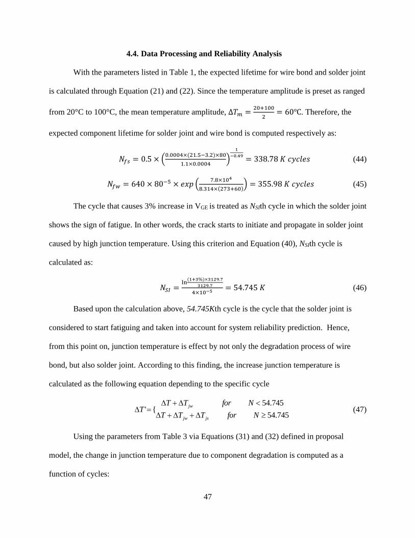
47
4.4. Data Processing and Reliability Analysis
With the parameters listed in Table 1, the expected lifetime for wire bond and solder joint
is calculated through Equation (21) and (22). Since the temperature amplitude is preset as ranged
from 20°C to 100°C, the mean temperature amplitude, ∆𝑇𝑚 =20+100
2= 60℃. Therefore, the
expected component lifetime for solder joint and wire bond is computed respectively as:
𝑁𝑓𝑠 = 0.5 × (0.0004×(21.5−3.2)×80
1.1×0.0004)
1
−0.49= 338.78 𝐾 𝑐𝑦𝑐𝑙𝑒𝑠 (44)
𝑁𝑓𝑤 = 640 × 80−5 × 𝑒𝑥𝑝 (7.8×10⁴
8.314×(273+60)) = 355.98 𝐾 𝑐𝑦𝑐𝑙𝑒𝑠 (45)
The cycle that causes 3% increase in VGE is treated as NSIth cycle in which the solder joint
shows the sign of fatigue. In other words, the crack starts to initiate and propagate in solder joint
caused by high junction temperature. Using this criterion and Equation (40), NSIth cycle is
calculated as:
𝑁𝑆𝐼 =ln
(1+3%)×3129.7
3129.7
4×10−5 = 54.745 𝐾 (46)
Based upon the calculation above, 54.745Kth cycle is the cycle that the solder joint is
considered to start fatiguing and taken into account for system reliability prediction. Hence,
from this point on, junction temperature is effect by not only the degradation process of wire
bond, but also solder joint. According to this finding, the increase junction temperature is
calculated as the following equation depending to the specific cycle
745.54
745.54{'
NforTTT
NforTTT
jsjw
jw (47)
Using the parameters from Table 3 via Equations (31) and (32) defined in proposal
model, the change in junction temperature due to component degradation is computed as a
function of cycles:

48
∆𝑇𝑗𝑤 =∆𝑉𝐶𝐸
2 𝑁
𝐼𝐶𝑤𝜌𝑤𝑣𝑤=
3129.7×𝑒4×10⁻⁵𝑁×𝑁
300×951×2869×0.004×2.5×0.004= 0.956 × 𝑒4×10⁻⁵𝑁 × 𝑁 (48)
∆𝑇𝑗𝑠 =∆𝑉𝐺𝐸
2𝑁
𝐼𝐶𝑠𝜌𝑠𝑣𝑠=
3975.4×𝑒0.0026×10⁻⁵𝑁×𝑁
300×7370×150×0.00695∗0.00645×0.001= 267.37 × 𝑒0.0026×10⁻⁵𝑁 × 𝑁 (49)
Therefore, the overall updated junction temperature is calculated using Equation (16) as
shown in Figure 18.
Figure 18. Increasing pattern of junction temperature during power cycling.
Based on observation from Figure 18, the junction temperature increase reveals the
impact of component degradation process on junction temperature as demonstrated by the slope
of the curve increase over the number of cycles. Clear increase on the curve is observed as power
cycling continues, which indicates the further component degradation process due to increase in
the junction temperature.
With the overall junction temperature updated at each cycle, the expected component
lifetime is calculated as:
𝑁𝑓𝑠′ = 0.5(
𝐿∆𝐶𝑇𝐸∆𝑇′
𝛾𝑥)1/𝑐 (50)
𝑁𝑓𝑤′ = 𝐴∆𝑇′𝛼𝑒𝑥𝑝 (
𝑄
𝑅𝑇𝑚) (51)

49
The lifetime data for both components are assumed to follow normal distribution since
normal distribution provides good fit to estimate the number of cycle to fail on component that
under constant or random amplitude loading conditions [37]-[40]. It is testified by plotting
fatigue life distributions in different probability papers and examining the goodness-of-fits of
these distributions with chi-square techniques [46]. For the purpose of simplicity, a fix
proportion 30% of the expected life is considered for the variance for both components. Hence,
the probabilistic model is updated with the increase junction temperature is given as:
𝑅′𝑠(𝑁)~𝑛𝑜𝑟𝑚{𝜇′𝑠(𝑁), 30%𝜇′𝑠2(𝑁)} (52)
𝑅′𝑤(𝑁)~𝑛𝑜𝑟𝑚{𝜇′𝑤(𝑁), 30%𝜇′𝑤2 (𝑁)} (53)
Based on Equations (39) and (40), the component reliability and system reliability are
calculated at every specific cycle. For example, in pth cycle, if p is less than NSI, the system
reliability is only dependent to the wire bond degradation process. Hence, the increase junction
temperature due to it is calculated as:
𝑇𝑗𝑤𝑝 = 0.956 × 𝑒4×10⁻⁵𝑁𝑝 × 𝑁𝑝 (54)
The overall junction temperature is computed as:
∆𝑇𝑝′ = ∆𝑇𝑗 + ∆𝑇𝑗𝑤𝑝 = ∆𝑇 + 0.956 × 𝑒4×10⁻⁵𝑁𝑝 × 𝑁𝑝 (55)
With the updated component lifetime on wire bond computed with Equation (10) as:
𝑁𝑓𝑤𝑝′ = 𝐴∆𝑇𝑝
′𝛼𝑒𝑥𝑝 (𝑄
𝑅𝑇𝑚) (56)
the system reliability of IGBT module, according to Equation (13), is computed as:
𝑅𝑠𝑦𝑠𝑡𝑒𝑚 = 𝑅′𝑤(𝑁 > 𝑁𝑤′ ) = 𝑛𝑜𝑟𝑚(𝑁𝑝 > 𝑁𝑓𝑤𝑝
′ ) (57)
However, if p is greater than NSI, the system reliability is not only dependent to the wire
bond degradation process, but also relies on the solder joint lifetime. Hence, the increase junction
temperature due to both components is calculated respectively as:

50
𝑇𝑗𝑤𝑝 = 0.956 × 𝑒4×10⁻⁵𝑁𝑝 × 𝑁𝑝 (58)
∆𝑇𝑗𝑠 = 267.37 × 𝑒0.0026×10⁻⁵𝑁𝑝 × 𝑁𝑝 (59)
The overall junction temperature is computed as:
∆𝑇𝑝′ = ∆𝑇𝑗 + ∆𝑇𝑗𝑤𝑝 + ∆𝑇𝑗𝑠
= ∆𝑇 + 0.956 × 𝑒4×10⁻⁵𝑁𝑝 × 𝑁𝑝 + 267.37 × 𝑒0.0026×10⁻⁵𝑁𝑝 × 𝑁𝑝 (60)
With the updated component lifetime on wire bond and solder joint computed with
Equation (33) (34) as:
𝑁𝑓𝑤𝑝′ = 𝐴∆𝑇𝑝
′𝛼𝑒𝑥𝑝 (𝑄
𝑅𝑇𝑚) (61)
𝑁𝑓𝑠𝑝′ = 0.5(
𝐿∆𝐶𝑇𝐸∆𝑇𝑝′
𝛾𝑥)1/𝑐 (62)
the system reliability of IGBT module, according to Equation (38), is computed as:
𝑅𝑠𝑦𝑠𝑡𝑒𝑚 = 𝑅′𝑤(𝑁 > 𝑁𝑤
′ ) × 𝑅′𝑠(𝑁 > 𝑁𝑠
′)
= 𝑛𝑜𝑟𝑚(𝑁𝑝 > 𝑁𝑓𝑤𝑝′ ) × 𝑛𝑜𝑟𝑚(𝑁𝑠 > 𝑁𝑓𝑠𝑝
′ ) (63)
With this computing algorithm, the system reliability and the component reliability are
computed at each cycle. The result is plotted in Figure 19. For the purpose of comparison, the
system reliability with independent assumption, which does not consider failure mechanism
interaction between crticial components, is also plotted in Figure 19.

51
Figure 19. Component reliability and system reliability.
In Figure 19, the system reliability with independent assumption and the system
reliability are represented in the red curve and the green curve respectively. Meanwhile, the
component reliability curves of wire bond and solder joint are marked in blue and brown
accordingly. All curves have a decreasing pattern as the numbers of cycles continue. Early
junction temperature increases is negligible and do not effect product lifetime since no sign of
obvious fatigue is observed from Figure 19. As power cycling continues, the wire bond starts to
fatigue as the blue curve declines after 150K cycles. Due to the increase junction temperature
and the failure mechanism interaction, the solder joint degradation process follows at 200K
cycles and both components’ degradation rates gradually rise especially after 250K cycles. The
wire bond reliability curve is under the solder joint reliability curve during this power cycling
test, meaning that the wire bond maintains its predominant failure mechanism and influences the
system reliability the most since it fails faster. This confirms the observation of the
predominance of wire bond failure mechanism when temperature amplitude is under 130K in
[34] [42] [44]. In such a case, reliability improvement on wire bonding area is critical and can
result in late initiation of wire bond degradation process, which potentially alleviate the mutual

52
effect of failure interaction and postpones the solder joint degradation. Therefore, the system
lifetime is enhanced and reliability is improved.
The system reliability with dependence and independence assumption are computed and
plotted in Figure 19 as well. At the beginning of power cycling, the green curve and the red
curve overlap with each other meaning there is no reliability prediction difference given only the
wire bond degradation process is involved. However, as power cycling continues, huge
discrepancy emerges. This phenomenon is noted when the solder joint degradation process
pitches in. From 190K cycles, at which solder joint starts to show recognizable drop on its
reliability curves, the distinct gap between the red curve and the green curve is observed
indicating the system is failing faster than it is predicted with the dependent assumption. With
the consideration of failure interaction, the green curve clearly shows that system degrades faster
than the red curve, meaning the proposed reliability method is able capture the interaction
between these two components’ failure mechanisms which the independent assumption fails to.
The effectiveness and accuracy of the proposed reliability method is amplified after 250K cycle,
at which the system is functioning in its most vulnerable state and the mutual effect of
component failure mechanisms interaction is magnified due to the rapid increase in junction
temperature. In Figure 18, junction temperature increases at faster rate after 250K cycles.
Meanwhile, in accordance, a sharp drop on system reliability after 250K cycles on the green
curve can be observed in Figure 19. Based upon this phenomenon, the significant influences of
the failure mechanism interaction and junction temperature on system reliability is demonstrated.
However, a smoother decreasing trend is shown on the red curve. Due to the assumption of
independence relationship between components, the potential component failure mechanism
interaction is not considered, which leads to invalid interpretation on system reliability especially

53
in the late stage of product life. Furthermore, the independence assumption computes the system
reliability as the product of the component reliabilities as a series configuration, the computing
result tends to emphasizes on the importance of the component that contributes a higher portion
in the calculation. In our case, it is the wire bond due to its predominant failure mechanism.
Reflected in Figure 19, the red curve is almost parallel to the blue curve after 290K cycles. The
reasoning above demonstrates the effectiveness and validity of the proposed reliability model
and the rationale of considering failure interaction to provide more realistic estimates of system
reliability. At the same time, reliability computation with the independence assumption might
overestimate the system reliability and lead to errors.
.

54
5. CONCLUSION
In this work, a reliability prediction model is proposed to compute the system reliability
of power electronic model capturing the failure mechanism interaction between critical
components: wire bond and solder joint. Wire bond and solder joint are important components
for thermal, mechanical and electrical connection in IGBT module. The component degradation
process is resulted from the stress strength caused by inhomogeneous component structure and
temperature amplitude during power cycling. Additionally, failure interaction between
component failure modes affects component failure characteristics and is never precisely
interpreted. However, most of the existing literatures fail to propose a comprehensive way to
deal with IGBT system reliability with the consideration of failure interaction between
components. Therefore, the interest of this work is inspired and further proceeded to provide a
realistic reliability assessment on PEM.
First, the degradation process of solder joint and wire bond is trigger due to the influence
of thermo-mechanical stress. The failure characteristics of solder joint and wire bond are
captured via selected PoF model respectively. Dependent to the impact that the effect of thermal
strains or temperature amplitude has on critical components many PoF models have been
established. To completely capture all the factors contributing to component degradation,
component physical dimensions and material properties are taken account. Second, PoF models
only estimate the average component lifetime. It does not provide any probabilistic interpretation
for reliability assessment. Component lifetime often has variation and follows a certain
distribution, which is more of the case in reality. In order to provide realistic reliability analysis,
the selected PoF models are converted into probabilistic models. Normal distribution is selected
to describe the failure characteristics of component degradation process because fatigue data can

55
be approximated as normal distribution under random or constant loading condition [37]. Third,
the failure interaction between wire bond and solder joint is studied. Wire bond lift-off is treated
as the predominant failure mode based upon observed experiments [10] [32] and solder joint
delamination is triggered by wire bond degradation process. Increased junction temperature is
captured as it is affected by the degradation process of both components. Additionally, both wire
bond and solder joint suffered increased thermo-mechanical stress as junction temperature rises.
Therefore, with updated junction temperature at each time, the expected component lifetime is
estimated. In the end, the system reliability is computed in a series system configuration.
Dataset abstracted from [6] [34] and [42] are mainly used to study the failure
characteristics of wire bond and solder joint for the contribution of the increase junction
temperature. In addition, 3% change has been used as threshold criteria for initiation phase for
solder joint. Nonlinear regression techniques via MINITAB have been used to develop the
individual models for wire bond and solder joint respectively. Through Joule’s law, the increased
junction temperature is computed based upon the regression models.
Reliability analysis was performed treating the system as a series configuration. System
reliability is divided and computed into two phases. In the first phase, only the failure
mechanism of wire bond is take account due to its predominance and solder joint not showing
any sign of fatigue. The system reliability is only dependent to the failure fatigue of wire bond.
The second phase begins when cracks initiated in solder joint. The system reliability is the
product of reliability of solder joint and wire bond. Compared to the system reliability with
independent assumption, the proposed model indicates earlier failure of the system. This
demonstrates the necessity of capturing failure interaction and the acceleration of failure
characteristics due the impact of failure interaction. From Figure 18, junction temperature

56
increases at a faster after 250K cycles. Accordingly, the system reliability has a faster drop after
250K cycles shown in Figure 19. This validates the choice of normal distribution for
probabilistic interpretation and the proposal model considering failure interaction between wire
bond and solder joint.
In future research, the proposal model needs to be enhanced for various operating
conditions incorporating various parameters. This allows more precise prediction on component
lifetime for a wider range of applicable situations. Design of experiment can be under taken to
find out the effective parameters if dataset is affluent. Comprehensive ANOVA approach can be
adopted to accurately model the statistical behavior of VCE and VGE for regression model. Use of
Bayesian model could be explored for a better insight into reliability behavior when fatigue data
is available.

57
REFERENCES
[1] H. Wang, "Toward Reliable Power Electronics: Challenges, Design Tools, and
Opportunities," Industrial Electronics Magazine, IEEE vol. 7.2, pp. 17-26, 2013.
[2] MIL-HDBK-217F, Reliability Prediction of Electronic Equipment, 1991. Notice 1 (1992) and
Notice 2 (1995).
[3] W. Nelson, Accelerated testing: statistical models, test plans, and data analysis. vol. 344.
John Wiley & Sons, 2009.
[4] H. Peng, et al., "Reliability and Maintenance Modeling for Systems Subject to Multiple
Dependent Competing Failure Processes," IIE transactions, vol. 43.1, pp. 12-22, 2010.
[5] H. A. Schafft, Testing and Fabrication of Wire-Bond Electrical Connections-A
Comprehensive Survey, No. NBS-TN-726. NATIONAL BUREAU OF STANDARDS
WASHINGTON DC ELECTRONIC TECHNOLOGY DIV, 1972.
[6] M. Held, et al,. "Fast Power Cycling Test for Insulated Gate Bipolar Transistor Modules in
Traction Application," International journal of electronics, vol. 86.10, pp. 1193-1204,
1999.
[7] A. Micol, et al., "An Investigation Into The Reliability of Power Modules Considering
Baseplate Solders Thermal Fatigue in Aeronautical Applications," Microelectronics
Reliability, vol. 49.9, pp. 1370-1374, 2009.
[8] A. Gurmukh and OP. Yadav, "A Unified Model Approach for Solder Joint Life Prediction,"
in Reliability and Maintainability Symposium (RAMS), Annual. IEEE, 2015, pp. 1-7.
[9] R. Amro, et al., "Power Cycling With High Temperature Swing of Discrete Components
Based On Different Technologies," in Power Electronics Specialists Conference, IEEE
35th Annual. Vol. 4. IEEE, 2004, pp. 2593-2598.

58
[10] L. Yang, et al., "Physics-of-Failure Lifetime Prediction Models for Wire Bond
Interconnects in Power Electronic Modules," Device and Materials Reliability, IEEE
Transactions on, vol. 13.1, pp. 9-17, 2013.
[11] SR-332, Reliability Prediction Procedure for Electronic Equipment, Telcordia, Issue 2,
September 2006.
[12] ITEM Software and ReliaSoft Corporation, RS 490 Course Notes: Introduction to
Standards Based Reliability Prediction and Lambda Predict, 2006.
[13] Y. Song, and B. Wang, "Survey on reliability of power electronic systems," Power
Electronics, IEEE Transactions on, vol. 28.1, pp. 591-604, 2013.
[14] W. Huang, "Reliability Analysis Considering Product Performance Degradation," Ph.D.
dissertation, Dept. Systems and Industrial Engineering, The University of Arizona, AZ,
2002.
[15] Z. Pan and N. Balakrishnan, "Reliability Modeling Of Degradation of Products With
Multiple Performance Characteristics Based on Gamma Processes," Reliability
Engineering & System Safety, vol. 96.8, pp. 949-957, 2011.
[16] K. Rafiee, et al., "Reliability Modeling for Dependent Competing Failure Processes With
Changing Degradation Rate." IIE Transactions, vol. 46.5, pp. 483-496, 2014.
[17] K. Yang and J. Xue, "Continuous State Reliability Analysis," Reliability and
Maintainability Symposium, 1996 Proceedings. International Symposium on Product
Quality and Integrity., Annual. IEEE, 1996, pp. 251-257.
[18] W. Huang and R.G. Askin, "Reliability Analysis of Electronic Devices With Multiple
Competing Failure Modes Involving Performance Aging Degradation," Quality and
Reliability Engineering International, vol. 19.3, pp. 241-254, 2003.

59
[19] J.A. Hoeting, et al., "Bayesian Model Averaging: A Tutorial," Statistical science, vol. 44.4,
pp. 382-401, 1999.
[20] H. Wang and J. Gao, "A Reliability Evaluation Study Based On Competing Failures for
Aircraft Engines," Eksploatacja i Niezawodność, vol. 16, 2014.
[21] Microelectronics Reliability: Physics-of-Failure Based Modeling and Lifetime Evaluation,
Jet Propulsion Laboratory, National Aeronautics and Space Administration, Pasadena,
CA, 2008.
[22] J. Goehre, et al., "Interface Degradation of Al Heavy Wire Bonds on Power Semiconductors
During Active Power Cycling Measured By The Shear Test," Integrated Power
Electronics Systems (CIPS), 2010 6th International Conference on. IEEE, 2010, pp. 1-6.
[23] J. Onuki, et al., "Reliability of Thick Al Wire Bonds in IGBT Modules for Traction Motor
Drives," Advanced Packaging, IEEE Transactions on, vol. 23.1, pp. 108-112, 2000.
[24] S. Ramminger, et al., "Crack Mechanism in Wire Bonding Joints," Microelectronics
Reliability, vol. 38.6, pp. 1301-1305, 1998.
[25] J.M. Göhre, “Development And Implementation of An Improved Load Change Test Method
for Experimental Determination of The Reliability of Thick Wire Bonds in Power
Modules,” Ph.D. dissertation, Dept. Electrical Engineering and computer science,
Technical University of Berlin, Berlin, Germany, 2013.
[26] W. Engelmaier, "Solder Joints in Electronics: Design For Reliability," Design and
Reliability of Solders and Solder Interconnections, RK Mahidhara, et. al., ed. The
Minerals, Metals & Materials Society, Warrendale, PA, pp: 9-19, Feb. 1997.
[27] W.W. Lee, et al., "Solder Joint Fatigue Models: Review and Applicability to Chip Scale
Packages," Microelectronics reliability, vol. 40.2, pp. 231-244, 2000.

60
[28] H.D. Solomon, "Fatigue of 60/40 solder," Components, Hybrids, and Manufacturing
Technology, IEEE Transactions on, vol. 9.4, pp. 423-432, 1986.
[29] H.S. Choi, et al., "Prediction of Reliability on Thermoelectric Module Through Accelerated
Life Test and Physics-of-Failure." Electronic Materials Letters, vol. 7.3, pp. 271-275,
2011.
[30] C.Y. Yin, et al., "A Physics-of-Failure Based Prognostic Method for Power Modules,"
Electronics Packaging Technology Conference, EPTC 10th. IEEE, 2008, pp. 1190-1195.
[31] G. Mitic, et al., "Reliability of AlN substrates and Their Solder Joints in IGBT Power
Modules," Microelectronics reliability, vol. 39.6, pp. 1159-1164, 1999.
[32] T.Y. Hung, et al., "Investigation of Solder Crack Behavior and Fatigue Life of the Power
Module on Different Thermal Cycling Period." Microelectronic Engineering, vol. 107,
pp. 125-129, 2013.
[33] Ciappa, M. "Selected failure mechanisms of modern power modules,” Microelectronics
reliability, vol. 42.4, pp. 653-667, 2002.
[34] A. Morozumi, et al., "Reliability of Power Cycling for IGBT Power Semiconductor
Modules," Industry Applications, IEEE Transactions on, vol. 39.3, pp. 665-671, 2003.
[35] L.F. Coffin, "A Study of The Effect of Cyclic Thermal Stresses on A Ductile
Metal." American Society of Mechanical Engineers, vol. 76, pp. 931-950, 1954.
[36] S.S. Manson, Behavior of Materials Under Conditions of Thermal Stress, TN 2933: NACA,
1953.
[37] V. Rathod, et al., "Probabilistic Modeling of Fatigue Damage Accumulation for Reliability
Prediction," International Journal of Quality, Statistics, and Reliability, 2011.

61
[38] P.H Wirsching and Y.N. Chen, "Considerations of Probability-Based Fatigue Design for
Marine Structures," Marine Structures, vol. 1.1, pp. 23-45, 1988.
[39] J.M. Bloom and J.C. Ekvall, Probabilistic Fracture Mechanics and Fatigue Methods:
Applications for Structural Design and Maintenance: A Symposium. No. 798. ASTM
International, 1983.
[40] W.F. Wu, et al., "Estimation of Fatigue Damage and Fatigue Life of Components Under
Random Loading," International Journal of Pressure Vessels and Piping, vol. 72.3, pp.
243-249, 1998.
[41] A. Hamidi, et al., "Reliability and Lifetime Evaluation of Different Wire Bonding
Technologies for High Power IGBT Modules," Microelectronics Reliability, vol. 39.6,
pp. 1153-1158, 1999.
[42] R. Amro, et al., "Power Cycling With High Temperature Swing of Discrete Components
Based on Different Technologies," in PESC 04. 2004 IEEE 35th Annual. Vol. 4, pp.
2593-2598, 2004.
[43] W. Wu, et al., "Investigation on the Long Term Reliability of Power IGBT Modules," in
Proceedings of the 7th International Symposium on. IEEE, 1995.
[44] U. Scheuermann, U. "Power Cycling Lifetime of Advanced Power Modules for Different
Temperature Swings,” in Proc. PCIM PE4. 5, Nürnberg 2002, pp. 59-64.
[45] J. R. Celaya, et al., "Prognostics Approach for Power MOSFET Under Thermal-Stress
Aging," in Proceedings Reliability and Maintainability Symposium 2012 Annual. IEEE,
2012.

62
[46] Y. Wang, et al., "A simulation of Intelligent Power Module under power cycling
condition," Electronic Packaging Technology (ICEPT), 2014 15th International
Conference on. IEEE, 2014.
[47] Gaiser Precision Bonding Tools, ”Fine-Pitch Capillary,” www.coorstek.com. Web. 09 Sep.
2015.
[48] J. Pang, et al., "Thermal cycling analysis of flip-chip solder joint reliability." Components
and Packaging Technologies, IEEE Transactions on, vol. 24.4, pp. 705-712, 2001.