A new semi-analytical solution for inertial waves in a rectangular parallelepipedS. Nurijanyan, O. Bokhove, and L. R. M. Maas Citation: Physics of Fluids (1994-present) 25, 126601 (2013); doi: 10.1063/1.4837576 View online: http://dx.doi.org/10.1063/1.4837576 View Table of Contents: http://scitation.aip.org/content/aip/journal/pof2/25/12?ver=pdfcov Published by the AIP Publishing

This article is copyrighted as indicated in the article. Reuse of AIP content is subject to the terms at: http://scitation.aip.org/termsconditions. Downloaded to IP:

130.89.13.208 On: Wed, 12 Feb 2014 14:09:18

PHYSICS OF FLUIDS 25, 126601 (2013)

A new semi-analytical solution for inertial waves in arectangular parallelepiped

S. Nurijanyan,1,a) O. Bokhove,1,2,b) and L. R. M. Maas3,c)

1Department of Applied Mathematics, University of Twente, P.O. Box 217, 7500 AE,Enschede, The Netherlands2School of Mathematics, University of Leeds, LS2 9JT Leeds, United Kingdom3NIOZ Royal Netherlands Institute for Sea Research, P.O. Box 59, 1790 AB, Den Burg,The Netherlands

(Received 13 November 2012; accepted 27 October 2013;published online 13 December 2013)

A study of inertial gyroscopic waves in a rotating homogeneous fluid is undertakenboth theoretically and numerically. A novel approach is presented to construct a semi-analytical solution of a linear three-dimensional fluid flow in a rotating rectangularparallelepiped bounded by solid walls. The three-dimensional solution is expandedin vertical modes to reduce the dynamics to the horizontal plane. On this horizontalplane, the two dimensional solution is constructed via superposition of “inertial”analogs of surface Poincare and Kelvin waves reflecting from the walls. The infinitesum of inertial Poincare waves has to cancel the normal flow of two inertial Kelvinwaves near the boundaries. The wave system corresponding to every vertical moderesults in an eigenvalue problem. Corresponding computations for rotationally modi-fied surface gravity waves are in agreement with numerical values obtained by Taylor[“Tidal oscillations in gulfs and basins,” Proc. London Math. Soc., Ser. 2 XX, 148–181 (1921)], Rao [“Free gravitational oscillations in rotating rectangular basins,” J.Fluid Mech. 25, 523–555 (1966)] and also, for inertial waves, by Maas [“On theamphidromic structure of inertial waves in a rectangular parallelepiped,” Fluid Dyn.Res. 33, 373–401 (2003)] upon truncation of an infinite matrix. The present approachenhances the currently available, structurally concise modal solution introduced byMaas. In contrast to Maas’ approach, our solution does not have any convergenceissues in the interior and does not suffer from Gibbs phenomenon at the bound-aries. Additionally, an alternative finite element method is used to contrast thesetwo semi-analytical solutions with a purely numerical one. The main differences arediscussed for a particular example and one eigenfrequency. C© 2013 AIP PublishingLLC. [http://dx.doi.org/10.1063/1.4837576]

I. INTRODUCTION

Fluid phenomena on Earth involve rotation to a greater or lesser extent. There are flows inwhich rotation is an absolutely essential factor. Waves that are appearing in a closed rotating con-tainer filled with a homogeneous fluid became a subject of interest to the scientific communityat the end of the 19th century and beginning of the 20th century. Taylor1 derived and presentedthe first complete linear solutions (valid for any angular frequency) for free surface oscillations ina rotating rectangular parallelepiped. Before Taylor, Rayleigh2 discussed the problem of the freetidal oscillations of a rectangular sea of uniform depth, when the vertical component of the Earth’srotation period is large compared with the periods of the oscillations. Later, the subject was studiedby Proudman,3, 4 who also corrected some inaccuracies and errors in Rayleigh’s works. A large

a)Electronic mail: s.nurijanyan@utwente.nlb)Electronic mail: o.bokhove@leeds.ac.ukc)Electronic mail: maas@nioz.nl

1070-6631/2013/25(12)/126601/21/$30.00 C©2013 AIP Publishing LLC25, 126601-1

This article is copyrighted as indicated in the article. Reuse of AIP content is subject to the terms at: http://scitation.aip.org/termsconditions. Downloaded to IP:

130.89.13.208 On: Wed, 12 Feb 2014 14:09:18

126601-2 Nurijanyan, Bokhove, and Maas Phys. Fluids 25, 126601 (2013)

amount of research has been focused on rotationally modified surface gravity waves as a majorrepresentative of the low-frequency waves in a homogeneous rotating fluid. In oceanography theseare referred to as Poincare and Kelvin waves, depending on whether the waves display a strictlysinusoidal or partially exponential spatial dependence (e.g., LeBlond and Mysak5). However, thereis a class of inertial (gyroscopic) waves that are possible within the interior of homogeneous rotatingfluids. Unlike the surface gravity waves, they have their maximum displacement in the interior ofthe domain, vanish at the free or solid surface, and are not affected by gravity. The frequenciesof these waves are below the inertial frequency, f = 2�, of the rotating domain, and they existsolely due to restoring Coriolis forces. No gravity effects are present in contrast to the case forsurface gravity waves. Pure inertial waves were initially discovered theoretically by Kelvin6 in acylindrical domain. The axial spheroid was the next geometry where the hyperbolic equation gov-erning the flow was solved by exactly satisfying the no-normal flow boundary conditions (Bryan7).Later, Maas8 presented a semi-analytical structural solution in a rectangular parallelepiped withstraight walls. Due to their symmetrical shape all three containers do not have any net focussingwhich inertial waves are otherwise prone to develop (Maas9). The axial spheroid has a symmet-ric structure, and thus compensates every reflected focussing wave with a reflected defocussingwave. In the case of an axial cylinder or a rectangular parallelepiped, the walls are either parallelor perpendicular to the rotation axis, therefore such walls possess a local reflectional symmetry.A simple tilt of one of the walls immediately results in symmetry breaking and hence in wavefocussing and defocussing, such that due to dominance of the former, wave attractors may appear(e.g., Maas9).

All the above mentioned theoretical solutions have also been observed experimentally. Inertialwaves were identified in a rotating axial cylinder by Fultz,10 McEwan,11 Manasseh,12, 13 Kobine,14

in a slightly tilted free surface cylinder by Thompson,15 in a sphere by Aldridge and Toomre,16 in atilted spheroid (tilt of its axis of rotation with respect to the axis of the cavity) by Malkus,17 Vanyoet al.,18 in a (truncated) cone by Beardsley,19 in a rectangular parallelepiped by Bewley et al.,20

Lamriben et al.,21 Boisson et al.,22 and in a trapezoid by Maas,9 Manders and Maas.23

From the theoretical point of view, the solutions for the inertial waves presented by Maas8 havea precise structure (revealed by use of the so-called Proudman-Rao method). The no-normal flowboundary conditions are satisfied exactly, by construction. Nevertheless, the solution is practicallyunusable, due to its poor convergence and Gibbs phenomenon at the boundaries, as shown inSec. II. We substitute the solution back into the linear Euler equations governing the flow andcalculate the residues. It appears that the residues of the momentum equations are not exactly zero,and moreover, their convergence to zero is very slow: with more than 200 Fourier modes, the residuestill is only of order 10−1 of the maximum flow. The convergence of the residue is faster in theinterior, in comparison to the boundaries, which is caused by the extra Gibbs phenomenon at theboundaries.

In this work, we present an enhanced solution for the free inertial waves of a rotating planar-rectangular parallelepiped, whose walls are parallel or perpendicular to the rotation axis. In Sec. II,we are presenting a detailed description of a new algorithm for the construction of this solution.As in Maas,8 the three-dimensional solution is reduced to a two-dimensional one, by assuming astanding mode structure in the vertical direction. Thus, for every vertical mode, the problem reducesto the horizontal plane, where the techniques introduced by Taylor1 for rotationally modified surfacegravity waves are used. The solution is sought as a superposition of inertial Poincare (IP) and inertialKelvin (IK) waves in the rectangular parallelepiped, the strictly rotational internal counterparts ofthe rotationally modified external gravity waves (Maas8). Two IK waves are chosen as a “base”or particular solutions for the flow in the horizontal plane. The IK waves are assumed to have nomotion in the x-direction (u = 0, v = v(x, y)), and thus they satisfy the no-normal flow boundaryconditions at x-walls, x = constant, automatically. IK waves grow exponentially in the along-wall,y-direction and are thus useful only when two opposite walls exist, excluding the unbounded growththat appears on infinite planes. Near the y-walls, the normal flow of these IK waves is compensatedby addition of an infinite sum of IP waves. In other words, we are searching a superposition of IK andIP waves such that the flow governed by them will not be disturbed by the presence of the solid wallsof the domain. The described algorithm (further called Taylor’s method) results in an eigenvalue

This article is copyrighted as indicated in the article. Reuse of AIP content is subject to the terms at: http://scitation.aip.org/termsconditions. Downloaded to IP:

130.89.13.208 On: Wed, 12 Feb 2014 14:09:18

126601-3 Nurijanyan, Bokhove, and Maas Phys. Fluids 25, 126601 (2013)

problem for an infinite matrix, the finite truncation of which identifies the eigenfrequencies. Thepresent algorithm has better convergence behaviour in the interior than the Proudman-Rao approachgiven by Maas:8 the residues of the momentum equations are exactly zero (up to machine precision).Results are discussed by comparing solutions of one particular eigenfrequency.

Nonetheless, the convergence of the solution is slow near the boundaries. Therefore, inSec. III, the problem is tackled purely from a numerical perspective by implementing a FiniteElement (FEM) discretisation of the governing linear Euler equations on the horizontal plane. Thecalculated numerical eigenfrequencies exactly coincide with the results of the above discussedsemi-analytical models. The differences between the numerical and the semi-analytical solutionsare analysed for one particular eigenfrequency. The numerical results verify the new semi-analyticaland FEM based methods. Conclusions are drawn in Sec. IV.

II. SEMI-ANALYTICAL INERTIAL WAVES IN A RECTANGULAR PARALLELEPIPED

A. 3D-to-2D reduction of governing equations

We consider a wave-tank (rectangular parallelepiped) with solid body rotation. The wave-tankhas fixed solid walls, is filled with an incompressible, homogenous fluid, and is rotating about avertical axis z∗ with a constant angular velocity �∗, perpendicular to two of its side walls. Below,asterisks denote dimensional quantities. We closely follow the notation of Maas.8 Small-amplitudemonochromatic waves appearing in the homogenous fluid on a rotating f∗-plane (f∗ = 2�∗) aregoverned by the linearised, inviscid equations of motion

∂u∗∂t∗

− f∗v∗ = − 1

ρ∗

∂ p∗∂x∗

, (1a)

∂v∗∂t∗

+ f∗u∗ = − 1

ρ∗

∂ p∗∂ y∗

, (1b)

∂w∗∂t∗

= − 1

ρ∗

∂ p∗∂z∗

, (1c)

∂u∗∂x∗

+ ∂v∗∂ y∗

+ ∂w∗∂z∗

= 0, (1d)

where (u∗, v∗, w∗) are the three-dimensional velocity components in the corresponding Cartesiandirections (x∗, y∗, z∗), p∗ is the linearised reduced pressure and ρ∗ is the density.

As in Maas,8 we consider standing modes in the vertical direction to make w∗ vanish at therigid bottom z∗ = −H∗ and top surface z∗ = 0, i.e.,

w∗ =∞∑

n=1

∂ζn∗∂t∗

sinnπ z∗

H∗, (2a)

(u∗, v∗, p∗) =∞∑

n=1

(un∗, vn∗, pn∗) cosnπ z∗

H∗, (2b)

where subscript n refers to the nth vertical mode, and where we discarded the degenerate(geostrophic) mode with n = 0, and hence w∗ = 0. The amplitude of the nth internal verticalelevation mode is denoted by ζ n∗. The presence of a solid wall at the top effectively eliminates thegravitational restoring forces and external gravity waves. Substitution of (2) into (1) modifies thegoverning equations in the following way:

∂un∗∂t∗

− f∗vn∗ = −Hn∗∂3ζn∗∂x∗∂t2∗

, (3a)

This article is copyrighted as indicated in the article. Reuse of AIP content is subject to the terms at: http://scitation.aip.org/termsconditions. Downloaded to IP:

130.89.13.208 On: Wed, 12 Feb 2014 14:09:18

126601-4 Nurijanyan, Bokhove, and Maas Phys. Fluids 25, 126601 (2013)

∂vn∗∂t∗

+ f∗un∗ = −Hn∗∂3ζn∗∂ y∗∂t2∗

, (3b)

∂ζn∗∂t∗

+ Hn∗

(∂u∗∂x∗

+ ∂v∗∂ y∗

)= 0, (3c)

with Hn∗ ≡ H∗/(nπ ) and pn∗ = ρ∗ Hn∗(∂2ζn∗/∂t2∗ ). For a specific nth vertical mode, (3) can be non-

dimensionalised with Hn∗ and f −1∗ as length and time scales as follows (u, v) = (un∗, vn∗)/(Hn∗ f∗):

ζ = ζ n∗/Hn∗, t = t∗f∗ and (x, y) = (x∗, y∗)/Hn∗. The dimensionless version of system (3) is

∂u

∂t− v = − ∂3ζ

∂x∂t2, (4a)

∂v

∂t+ u = − ∂3ζ

∂y∂t2, (4b)

∂ζ

∂t+ ∂u

∂x+ ∂v

∂y= 0. (4c)

After substitution of (u, v, ζ ) ∝ exp(−iσ t), system (4) becomes

(� + κ2)(u, v, ζ ) = 0, (5)

where σ is the frequency of monochromatic waves, κ is defined by κ2 = 1/σ 2 − 1, and the Laplacianis the following � = ∂xx + ∂yy. Thus, the horizontal spatial structure of monochromatic waves isdetermined by the Helmholtz equation (5).

After choosing the ansatz (2), the three-dimensional problem for resolving the flow (u, v, w, p)transforms into a two-dimensional (u, v, ζ ) problem in the two-dimensional container, defined inthe region 0 ≤ x ≤ L, −Y ≤ y ≤ Y. Therefore, we are looking for a solution which will satisfy (5)with no-normal flow boundary conditions at the four walls: u = 0 at x = 0 and x = L, and v = 0 aty = −Y and y = Y. Recall that, because of the mode (n) dependent scaling, the boundary sizes, L =nπL∗/H∗ and Y = nπY∗/H∗ also depend on this mode number.

As was already mentioned before, the solution provided via the Proudman-Rao method in Maas8

satisfies the boundary conditions by construction, but suffers from poor convergence in the interiorand Gibbs phenomenon at the boundaries. While some of the eigenfrequencies have indeed beenobtained experimentally (Bewley et al.20 and Lamriben et al.21) validating the precise shape of thecorresponding eigenmodes has been more cumbersome (Boisson et al.22). This may of course bepartially due to viscous boundary layers modifying the flow field near the boundaries, but may alsopartly be due to this convergence problem. The latter suggests that the development of a more precisemethod is desirable.

B. Taylor’s method

We will present an alternative solution for determining the horizontal flow of the nth verticalmode in a rectangular parallelepiped. The method of Taylor is using a combination of resultsdiscussed in Maas8 concerning inertial Poincare waves and inertial Kelvin waves. Thus, the algorithmis applicable to semi-infinite as well as finite rectangular regions. The idea is as follows: wesearch for analytic solutions of the Helmholtz equations (5), which do not or only partially satisfyimpermeability conditions at the boundary, but the superposition of which will meet the requirementsat the boundaries. To construct the final solution, we use a combination of two IK and numerous IPwaves defined in a finite meridional channel, available from Maas.8 The IK wave solution of (4) for

This article is copyrighted as indicated in the article. Reuse of AIP content is subject to the terms at: http://scitation.aip.org/termsconditions. Downloaded to IP:

130.89.13.208 On: Wed, 12 Feb 2014 14:09:18

126601-5 Nurijanyan, Bokhove, and Maas Phys. Fluids 25, 126601 (2013)

a finite meridional channel is given by

u = 0, (6a)

v = V exp

[−y + i

x − L/2

σ− iσ t

], (6b)

ζ = iv

σ. (6c)

Obviously, the latter wave satisfies no-normal flow boundary condition only in the x-direction.Meanwhile, IP waves with quantised wave-numbers {km = mπ /L}, m ∈ {1, 2, 3, ...} are given by

u = vmikmσ 3

1 − σ 2

[1 +

(lm

σkm

)2]

sin km x exp i(lm y − σ t), (7a)

v = vm

(−lmσ cos km x + 1

kmsin km x

)exp i(lm y − σ t), (7b)

ζ = vm(cos km x + lm

σkmsin km x) exp i(lm y − σ t), (7c)

where km = (km, lm) is the two-dimensional wave number vector and lm = ±(σ−2 − σ−2m )1/2

≡ −ism is determined by frequency σ , wave number km and σm = (1 + k2m)−1/2. These waves,

however, do not satisfy the boundary conditions v = 0 at y = ±Y, but by contrast do satisfy u = 0at x = 0, L.

After dropping the common factor exp(−iσ t), a solution of the Helmholtz equation (5), ex-pressed in terms of the meridional velocity v, is now supposed to consist of two IK waves that aretrapped at the walls y = ±Y, and of an infinite sum of channel IP waves, a finite number of whichare free to propagate in the y-direction:

2v = v+exp(i(x − L/2)/σ − y) + v−exp(−i(x − L/2)/σ + y) ++∞∑

m=−∞,m �=0

vm(ismσ cos km x + 1

kmsin km x)exp(sm y). (8)

In view of the definition of σ m, we find: 1 > σ 1 > σ 2 > . . . . Now, if our frequency σ lies in betweentwo of these eigenfrequencies: σ M > σ > σ M + 1, then the sm are imaginary for all m ≤ M, while theyare real for m > M. This implies that the first M modes have real lm. Since lm represent wave numbers,this implies M propagating modes, while all modes having m > M are trapped (real sm). For negativem, we define s−m = −sm and k−m = km. Positive m refers either to energy propagation in positivey-direction, or trapping to y = Y (depending on whether σ is larger or smaller than σ m). Negative mrefers to energy propagation in negative y-direction, or trapping to y = −Y. When we look for wavesthat are symmetric under reflection in the centre, (x, y) → (L − x, −y), the expression for v has to beinvariant under this transformation. This requires v− = v+ ≡ v0, v2m = −v−2m , v2m+1 = v−(2m+1).When we look for antisymmetric velocity fields v, these relations should reverse parity (v− = −v+,etc.). Consider now v-symmetric solutions and adopt a Cartesian coordinate frame ξ , y, whose originis at the centre of the rectangle, where

ξ = πx

L− π

2. (9)

The container is now restricted to ξ ∈ [−π /2, π /2]. Then, with

α ≡ L

πσ, (10)

This article is copyrighted as indicated in the article. Reuse of AIP content is subject to the terms at: http://scitation.aip.org/termsconditions. Downloaded to IP:

130.89.13.208 On: Wed, 12 Feb 2014 14:09:18

126601-6 Nurijanyan, Bokhove, and Maas Phys. Fluids 25, 126601 (2013)

the v-velocity can be expressed

v = cosh y cos αξ − i sinh y sin αξ +L

π

∞∑m odd

(−1)m−1

2 vm(−ism

αsin mξ sinh sm y + 1

mcos mξ cosh sm y) +

L

π

∞∑m even

(−1)m2 vm(i

sm

αcos mξ cosh sm y + 1

msin mξ sinh sm y), (11)

where the amplitude v0 has been arbitrarily set equal to one. Here and in the following all integersoccurring in summations are strictly positive. Notice the point symmetry of (11) as it is invariantunder the transformation (ξ , y) → (−ξ , −y). The IK waves (the first two terms in (11)) providea coupling between the IP waves, but numbers α should be non-integer, as the IK-waves wouldotherwise be exactly annihilated by one of the IP-waves (having sm = 1). Eigenfrequencies andamplitudes of each of the terms in (11) follow by rewriting this expression and by application of theboundary condition at y = ±Y.

The IK waves, possessing non-integer α, yield only the cosine of even and the sine of oddmultiples of ξ in their Fourier representations, as in the case of reflecting Kelvin waves (Taylor1):

cos αξ = 4α

πsin

(απ

2

) [1

2α2+

∑m even

(−1)m2

α2 − m2cos mξ

], (12a)

sin αξ = −4α

πcos

(απ

2

) ∑m odd

(−1)m−1

2

α2 − m2sin mξ . (12b)

These are, therefore, unable to match the cosine of odd and sine of even multiples of ξ , also oc-curring in (11). Now, we directly expand the terms cos αξ and sin αξ in (11) using (12) in cosineof even and sine of odd multiples of ξ , respectively, and require the coefficients of each of thetrigonometric terms to vanish separately at y = Y. The same conditions are obtained by applica-tion of the boundary condition at the opposing boundary y = −Y. However, this direct approachyields an unwieldy matrix equation. Probably for this reason, Taylor extended (12a) with odd and(12b) with even multiplies ξ . The cosine expansion in (12a), for instance, is extended with cos sξ(s odd), while each such term is counterbalanced by subtracting its even Fourier expansion (inanother application of (12a) to odd integers such that in effects zeroes are added). Each such oddmultiple and its counterbalancing Fourier expansion has an undetermined magnitude βs (s odd).For the sine expansion similar terms are added yielding undetermined magnitude γ s (s even). Theseundetermined magnitudes βs and γ s can be obtained from the requirement that the total velocityfield v vanishes at y = ±Y. The total velocity at y = Y reads

v(ξ, Y ) = 4α

πcosh Y sin

(απ

2

)[1

2α2+

∞∑m even

(−1)m2

α2 − m2cos mξ

+∞∑

s odd

βs

((−1)

s−12

π

4scos sξ −

( 1

2s2+

∞∑j even

(−1)j2

s2 − j2cos jξ

))]

+ i4α

πsinh Y cos

(απ

2

)[ ∞∑

m odd

(−1)m−1

2

α2 − m2sin mξ +

∞∑s even

γs

((−1)

s2π

4ssin sξ +

∞∑j odd

(−1)j−12

s2 − j2sin jξ

)]

This article is copyrighted as indicated in the article. Reuse of AIP content is subject to the terms at: http://scitation.aip.org/termsconditions. Downloaded to IP:

130.89.13.208 On: Wed, 12 Feb 2014 14:09:18

126601-7 Nurijanyan, Bokhove, and Maas Phys. Fluids 25, 126601 (2013)

+ L

π

∞∑m odd

(−1)m−1

2 vm(−ism

αsin mξ sinh smY + 1

mcos mξ cosh smY )

+ L

π

∞∑m even

(−1)m2 vm(i

sm

αcos mξ cosh smY + 1

msin mξ sinh smY ). (13)

Vanishing of this expression requires the separate vanishing of the coefficients of cos mξ or sin mξ .For m odd, vanishing of the coefficient of cos mξ requires

vm = −απ

L

cosh Y

cosh smYsin

(απ

2

)βm . (14)

On the other hand, vanishing of the coefficient of sin mξ requires

vm = 4α2

sm L

sinh Y

sinh smYcos

(απ

2

) [1

α2 − m2−

∞∑s even

γs

m2 − s2

]. (15)

The equality of these two expressions for vm determines βm in terms of γ s,

1

m2 − α2+

∞∑s even

γs

m2 − s2+ βmλm = 0, (16)

where

λm = − smπ

4αcoth Y tan

(απ

2

)tanh(smY ). (17)

For m even, we similarly find that vanishing of the coefficient of sin mξ requires

vm = −iαπ

L

sinh Y

sinh smYcos

(απ

2

)γm . (18)

Dividing this by the expression for vm obtained from vanishing of the coefficient of cos mξ one finds

− 1

m2 − α2+

∞∑s odd

βs

m2 − s2+ γmμm = 0, (19)

where

μm = smπ

4αtanh Y cot

(απ

2

)coth(smY ). (20)

If we define μ0 = 0, (19) also includes, for m = 0, the extra requirement that the constant term in(13) vanishes. Note that in the expressions for λm and μm, sm occurs in product with either tanh smyor coth sm y. The replacement sm = ilm when σ < σ m, and the property tanh iz = itanh z (for realz), therefore leaves these expressions real, regardless of whether sm is real or imaginary, making acumbersome sign-distinction (as in Taylor1) unnecessary. It also guarantees λm and μm (and thereforethe eigenfrequencies) to be real. Interpreting each first term of (16) and (19) as multiplying a quantityγ 0(= 1), the set of equations forms a system of infinite matrix equations Ac = 0, where A is as follows

A =

⎛⎜⎜⎜⎜⎜⎜⎜⎜⎜⎜⎜⎝

1α2

−112 0 −1

32 0 ...

112−α2 λ1

112−22 0 1

12−42 ...

−122−α2

122−12 μ2

122−32 0 ...

132−α2 0 1

32−22 λ31

32−42 ...

.

.

.

⎞⎟⎟⎟⎟⎟⎟⎟⎟⎟⎟⎟⎠

(21)

and column vector c = (γ 0, β1, γ 2, β3, ...)T, where superscript T means transpose. Matrix A istwice as big as the matrix obtained when directly expanding the terms in (11), alluded to above, but

This article is copyrighted as indicated in the article. Reuse of AIP content is subject to the terms at: http://scitation.aip.org/termsconditions. Downloaded to IP:

130.89.13.208 On: Wed, 12 Feb 2014 14:09:18

126601-8 Nurijanyan, Bokhove, and Maas Phys. Fluids 25, 126601 (2013)

is much simpler to handle. Apart from differences in the definitions of the diagonal terms λm andμm, together with the fact that our α is a function of frequency, (10), the matrix equation exactlyconforms with Taylor’s. Nontrivial solutions result only when its determinant vanishes, detA = 0,which (through α) can be regarded as an equation establishing eigenfrequencies σ . Amplitudes βm

(m is odd) and γ m (m is even), for any particular σ j, j = 1, 2... can be determined by the inversionof the reduced matrix that can be obtained from (16) and (19), where we now exclude the first row,corresponding to m = 0, and bring the first column to the right of the equation, which can nowbe regarded as known. With these amplitudes, from (15) and (18), also the amplitudes vm in theexpansion of v, Eq. (11), are determined, and the solution is in essence complete. We also note thatsimilar expressions can be obtained for antisymmetric solutions, where

λm = − smπ

4αtanh Y tan

(απ

2

)coth(smY ), (22a)

μm = smπ

4αcoth Y cot

(απ

2

)tanh(smY ) (22b)

and making similar replacements, sinh Y ⇐⇒−cosh Y and sinh smY ⇐⇒ cosh smY, in coefficientsvm and again, but with regards to the y-dependence, in fields u, v, and ζ .

For each eigenvalue and corresponding set of amplitudes vm , the velocity and elevation fieldsare now determined. Hence, the u velocity component of infinite sum of IP waves (7), with theircorresponding eigenvalue and set of amplitudes vm , reads

u =∞∑

m odd

i(−1)m−1

2 vm

( α

m− m

α

)cos mξ cosh sm y

+∞∑

m even

i(−1)m2 vm

( α

m− m

α

)sin mξ sinh sm y. (23)

The vertical elevation field then follows from the continuity equation

ζ = −σ−1

(∂u

∂x+ ∂v

∂y

)= −iσ−1(π L−1uξ + vy) = −σ−1(i sinh y cos αξ + cosh y sin αξ )

−∞∑

m odd

i(−1)m−1

2 vm

(sin mξ cosh sm y + iαsm

mcos mξ sinh sm y

)

+∞∑

m even

i(−1)m2 vm

(cos mξ sinh sm y − iαsm

msin mξ cosh sm y

). (24)

The eigenfrequencies are determined by truncating the infinite matrix to include just N rows andcolumns. Finding the roots of the resulting determinant numerically, and observing convergenceof these roots upon increase of the number of rows, the set of eigenfrequencies σ j, j = 1, 2... isdetermined (approximately).

C. Comparison of two methods: Taylor’s method vs. Proudman-Rao method

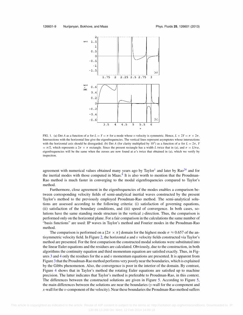
Next, this novel Taylor’s method for a construction of semi-analytical solutions for the lin-earised Euler equations in a rectangular parallelepiped is tested and verified from a numericalperspective. First a few eigenfrequencies are determined in a given [π × 2π ] rectangle, seeFigure 1. Also, an independent verification is performed by comparing the latter eigenfrequenciesto the frequencies for a [2π × π ] rectangle in Figure 1. The eigenfrequency of the first symmetricmode is σ ∗

1 = L/πα1 ≈ 0.657, which corresponds to the first root in Figure 1(a), at α1 ≈ 1.522.The next two eigenfrequencies of symmetric velocity modes are σ ∗

2 = L/πα1 ≈ 0.477, α2 ≈ 2.095and σ ∗

3 = L/πα1 ≈ 0.398, α3 ≈ 2.513. Numerical computations for the frequencies and modalstructures are assessed for several antisymmetric and symmetric modes. The eigenfrequencies andeigenmodes computed in this manner for the rotationally modified surface gravity modes are in

This article is copyrighted as indicated in the article. Reuse of AIP content is subject to the terms at: http://scitation.aip.org/termsconditions. Downloaded to IP:

130.89.13.208 On: Wed, 12 Feb 2014 14:09:18

126601-9 Nurijanyan, Bokhove, and Maas Phys. Fluids 25, 126601 (2013)

FIG. 1. (a) Det A as a function of α for L = Y = π for a mode whose v-velocity is symmetric. Hence, L × 2Y = π × 2π .Intersections with the horizontal line give the eigenfrequencies. The vertical lines represent asymptotes whose intersectionswith the horizontal axis should be disregarded. (b) Det A (for clarity multiplied by 103) as a function of α for L = 2π , Y= π /2, which represents a 2π × π rectangle. Since the present rectangle has a width L twice that in (a), and σ = L/πα,eigenfrequencies will be the same when the zeroes are now found at α’s twice that obtained in (a), which we verify byinspection.

agreement with numerical values obtained many years ago by Taylor1 and later by Rao24 and forthe inertial modes with those computed in Maas.8 It is also worth to mention that the Proudman-Rao method is much faster in converging to the modal eigenfrequencies compared to Taylor’smethod.

Furthermore, close agreement in the eigenfrequencies of the modes enables a comparison be-tween corresponding velocity fields of semi-analytical inertial waves constructed by the presentTaylor’s method to the previously employed Proudman-Rao method. The semi-analytical solu-tions are assessed according to the following criteria: (i) satisfaction of governing equations,(ii) satisfaction of the boundary conditions, and (iii) speed of convergence. In both cases, so-lutions have the same standing mode structure in the vertical z-direction. Thus, the comparison isperformed only on the horizontal plane. For a fair comparison in the calculations the same number of“basis functions” are used: IP waves in Taylor’s method and Fourier modes in the Proudman-Raomethod.

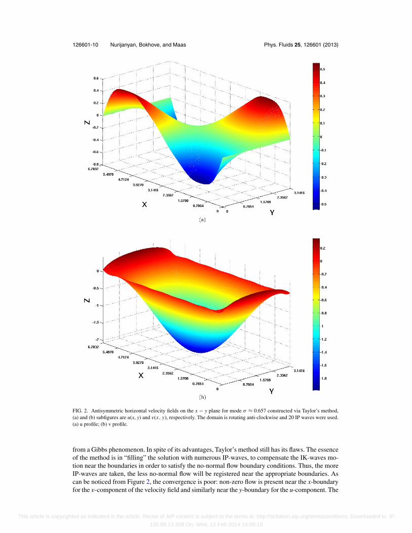
The comparison is performed on a [2π × π ] domain for the highest mode σ ≈ 0.657 of the an-tisymmetric velocity field. In Figure 2, the horizontal u and v velocity fields constructed via Taylor’smethod are presented. For the first comparison the constructed modal solutions were substituted intothe linear Euler equations and the residues are calculated. Obviously, due to the construction, in bothalgorithms the continuity equation and third momentum equation are satisfied exactly. Thus, in Fig-ures 3 and 4 only the residues for the u and v momentum equations are presented. It is apparent fromFigure 3 that the Proudman-Rao method performs very poorly near the boundaries, which is explainedby the Gibbs phenomenon. Also, the convergence is poor in the interior of the domain. By contrast,Figure 4 shows that in Taylor’s method the rotating Euler equations are satisfied up to machineprecision. The latter indicates that Taylor’s method is preferable to Proudman-Rao, in this context.The differences between the constructed solutions are given in Figure 5. According to Figure 5,the main differences between the solutions are near the boundaries (y-wall for the u-component andx-wall for the v-component of the velocity). Near these boundaries the Proudman-Rao method suffers

This article is copyrighted as indicated in the article. Reuse of AIP content is subject to the terms at: http://scitation.aip.org/termsconditions. Downloaded to IP:

130.89.13.208 On: Wed, 12 Feb 2014 14:09:18

126601-10 Nurijanyan, Bokhove, and Maas Phys. Fluids 25, 126601 (2013)

FIG. 2. Antisymmetric horizontal velocity fields on the x − y plane for mode σ ≈ 0.657 constructed via Taylor’s method,(a) and (b) subfigures are u(x, y) and v(x, y), respectively. The domain is rotating anti-clockwise and 20 IP waves were used.(a) u profile; (b) v profile.

from a Gibbs phenomenon. In spite of its advantages, Taylor’s method still has its flaws. The essenceof the method is in “filling” the solution with numerous IP-waves, to compensate the IK-waves mo-tion near the boundaries in order to satisfy the no-normal flow boundary conditions. Thus, the moreIP-waves are taken, the less no-normal flow will be registered near the appropriate boundaries. Ascan be noticed from Figure 2, the convergence is poor: non-zero flow is present near the x-boundaryfor the v-component of the velocity field and similarly near the y-boundary for the u-component. The

This article is copyrighted as indicated in the article. Reuse of AIP content is subject to the terms at: http://scitation.aip.org/termsconditions. Downloaded to IP:

130.89.13.208 On: Wed, 12 Feb 2014 14:09:18

126601-11 Nurijanyan, Bokhove, and Maas Phys. Fluids 25, 126601 (2013)

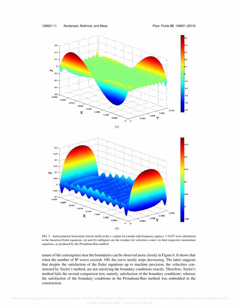
FIG. 3. Antisymmetric horizontal velocity fields in the x–y plane for a mode with frequency sigma σ ≈ 0.657 were substitutedin the linearised Euler equations. (a) and (b) subfigures are the residues for velocities u and v in their respective momentumequations, as produced by the Proudman-Rao method.

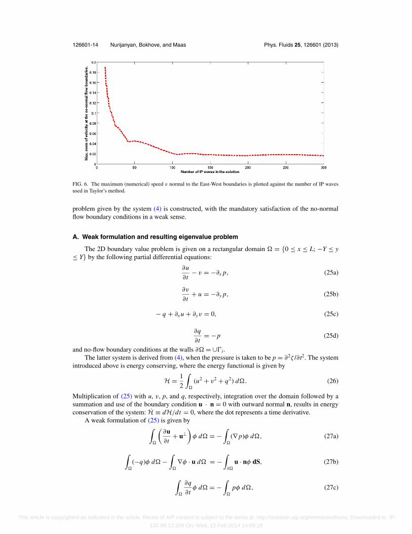
nature of the convergence near the boundaries can be observed more closely in Figure 6. It shows thatwhen the number of IP waves exceeds 100, the curve nearly stops decreasing. The latter suggeststhat despite the satisfaction of the Euler equations up to machine precision, the velocities con-structed by Taylor’s method, are not satisfying the boundary conditions exactly. Therefore, Taylor’smethod fails the second comparison test, namely, satisfaction of the boundary conditions; whereasthe satisfaction of the boundary conditions in the Proudman-Rao method was embedded in theconstruction.

This article is copyrighted as indicated in the article. Reuse of AIP content is subject to the terms at: http://scitation.aip.org/termsconditions. Downloaded to IP:

130.89.13.208 On: Wed, 12 Feb 2014 14:09:18

126601-12 Nurijanyan, Bokhove, and Maas Phys. Fluids 25, 126601 (2013)

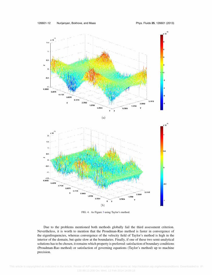
FIG. 4. As Figure 3 using Taylor’s method.

Due to the problems mentioned both methods globally fail the third assessment criterion.Nevertheless, it is worth to mention that the Proudman-Rao method is faster in convergence ofthe eigenfrequencies, whereas convergence of the velocity field of Taylor’s method is high in theinterior of the domain, but quite slow at the boundaries. Finally, if one of these two semi-analyticalsolutions has to be chosen, it remains which property is preferred: satisfaction of boundary conditions(Proudman-Rao method) or satisfaction of governing equations (Taylor’s method) up to machineprecision.

This article is copyrighted as indicated in the article. Reuse of AIP content is subject to the terms at: http://scitation.aip.org/termsconditions. Downloaded to IP:

130.89.13.208 On: Wed, 12 Feb 2014 14:09:18

126601-13 Nurijanyan, Bokhove, and Maas Phys. Fluids 25, 126601 (2013)

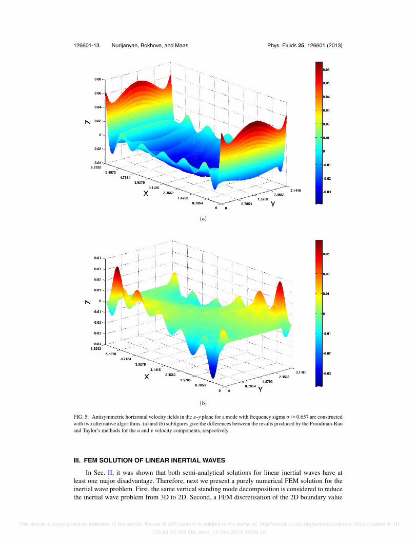
FIG. 5. Antisymmetric horizontal velocity fields in the x–y plane for a mode with frequency sigma σ ≈ 0.657 are constructedwith two alternative algorithms. (a) and (b) subfigures give the differences between the results produced by the Proudman-Raoand Taylor’s methods for the u and v velocity components, respectively.

III. FEM SOLUTION OF LINEAR INERTIAL WAVES

In Sec. II, it was shown that both semi-analytical solutions for linear inertial waves have atleast one major disadvantage. Therefore, next we present a purely numerical FEM solution for theinertial wave problem. First, the same vertical standing mode decomposition is considered to reducethe inertial wave problem from 3D to 2D. Second, a FEM discretisation of the 2D boundary value

This article is copyrighted as indicated in the article. Reuse of AIP content is subject to the terms at: http://scitation.aip.org/termsconditions. Downloaded to IP:

130.89.13.208 On: Wed, 12 Feb 2014 14:09:18

126601-14 Nurijanyan, Bokhove, and Maas Phys. Fluids 25, 126601 (2013)

FIG. 6. The maximum (numerical) speed v normal to the East-West boundaries is plotted against the number of IP wavesused in Taylor’s method.

problem given by the system (4) is constructed, with the mandatory satisfaction of the no-normalflow boundary conditions in a weak sense.

A. Weak formulation and resulting eigenvalue problem

The 2D boundary value problem is given on a rectangular domain � = {0 ≤ x ≤ L; −Y ≤ y≤ Y} by the following partial differential equations:

∂u

∂t− v = −∂x p, (25a)

∂v

∂t+ u = −∂y p, (25b)

− q + ∂x u + ∂yv = 0, (25c)

∂q

∂t= −p (25d)

and no-flow boundary conditions at the walls ∂� = ∪�i.The latter system is derived from (4), when the pressure is taken to be p = ∂2ζ /∂t2. The system

introduced above is energy conserving, where the energy functional is given by

H = 1

2

∫�

(u2 + v2 + q2) d�. (26)

Multiplication of (25) with u, v, p, and q, respectively, integration over the domain followed by asummation and use of the boundary condition u · n = 0 with outward normal n, results in energyconservation of the system: H ≡ dH/dt = 0, where the dot represents a time derivative.

A weak formulation of (25) is given by∫�

(∂u∂t

+ u⊥)

φ d� = −∫

�

(∇ p)φ d�, (27a)

∫�

(−q)φ d� −∫

�

∇φ · u d� = −∫

∂�

u · nφ dS, (27b)

∫�

∂q

∂tφ d� = −

∫�

pφ d�, (27c)

This article is copyrighted as indicated in the article. Reuse of AIP content is subject to the terms at: http://scitation.aip.org/termsconditions. Downloaded to IP:

130.89.13.208 On: Wed, 12 Feb 2014 14:09:18

126601-15 Nurijanyan, Bokhove, and Maas Phys. Fluids 25, 126601 (2013)

where the velocity field is given in terms of the two-dimensional vector u = (u, v)T , the perpendicularvelocity vector is u⊥ = (−v, u)T , the two-dimensional differential operator is ∇ = (∂/∂x, ∂/∂y)T

and φ is a test function taken from H 10 (�). Hence, the function spaces are chosen to be

H 10 (�) = {v ∈ H 1(�) : v = 0 on ∂�}, with (28a)

H 1(�) = {v ∈ L2(�) :∂v

∂x,∂v

∂y∈ L2(�)}, (28b)

where L2 is a space of square integrable functions.Note that after multiplication with a test function φ, we only do integration by parts in the

continuity equation, and skip the integration by parts in the momentum equation, which is a slightmodification of a classical FEM weak formulation. This way we ensure the conservation of theenergy on the discrete level, as shown later. The latter is crucial for an accurate and robust numericalscheme.

After taking into an account no flow boundary conditions u · n = 0 at ∂�, (27) becomes∫�

(∂u∂t

+ u⊥)

φ d� = −∫

�

(∇ p)φ d�, (29a)

∫�

(−q)φ d� −∫

�

∇φ · u d� = 0, (29b)

∫�

∂q

∂tφ d� = −

∫�

pφ d�. (29c)

Given a tessellation Ih of the domain �, we search for a weak solution of system (29) in

Vh = {v : v is continuous on �, v|K ∈ Pd (K ) ∀K ∈ Ih} ⊂ H 1(�), (30)

with Pd (K ) the space of polynomials of at most degree d on K ∈ Ih , where d ≥ 0. Variables u, v, p,q are represented via their expansions in terms of basis functions

u = uiφi , p = piφi , q = qiφi , (31)

where φi ∈ Vh and ui , pi, qi are expansion coefficients. We note that, here and hereafter, we use theEinstein convention implying summation over repeated indices. Incorporation of (31) into the weakformulation (29) results in

Mi j u j + Mi j u⊥j = −Si j p j , (32a)

Mi j q j + S j i · u j = 0, (32b)

Mi j q j = −Mi j p j , (32c)

where Mi j = ∫Ih

φiφ j dx, Si j = (Sxi j , Sy

i j )T = ∫

Ihφi∇φ j dx. If we multiply the discrete momentum

equation with ui , the continuity equation with pi, (32c) with qi and sum over all nodes, we willobtain the following equation

d

dt

(1

2

(Mi j ui · u j + Mi j qi q j

) )= 0, (33)

which ensures the conservation of a discrete energy functional in time, in addition to the conservationat the continuous level.

The unknowns pj and qj can be eliminated from (32): when a time derivative of (32b) is takenand the results are substituted into (32a) while using (32c), we obtain

Mi j u j + Sxil M−1

lk Sxjk u j + Sx

il M−1lk Sy

jk v j = Mi jv j , (34a)

Mi j v j + Syil M−1

lk Sxjk u j + Sy

il M−1lk Sy

jk v j = −Mi j u j . (34b)

This article is copyrighted as indicated in the article. Reuse of AIP content is subject to the terms at: http://scitation.aip.org/termsconditions. Downloaded to IP:

130.89.13.208 On: Wed, 12 Feb 2014 14:09:18

126601-16 Nurijanyan, Bokhove, and Maas Phys. Fluids 25, 126601 (2013)

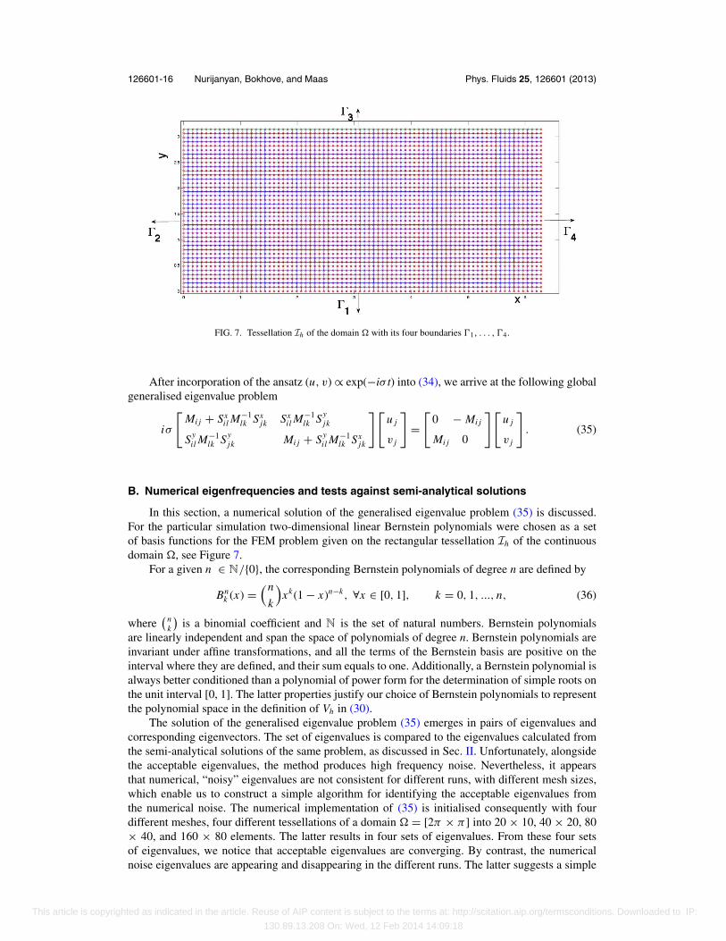
FIG. 7. Tessellation Ih of the domain � with its four boundaries �1, . . . , �4.

After incorporation of the ansatz (u, v) ∝ exp(−iσ t) into (34), we arrive at the following globalgeneralised eigenvalue problem

iσ

[Mi j + Sx

il M−1lk Sx

jk Sxil M−1

lk Syjk

Syil M−1

lk Syjk Mi j + Sy

il M−1lk Sx

jk

] [u j

v j

]=

[0 − Mi j

Mi j 0

][u j

v j

]. (35)

B. Numerical eigenfrequencies and tests against semi-analytical solutions

In this section, a numerical solution of the generalised eigenvalue problem (35) is discussed.For the particular simulation two-dimensional linear Bernstein polynomials were chosen as a setof basis functions for the FEM problem given on the rectangular tessellation Ih of the continuousdomain �, see Figure 7.

For a given n ∈ N/{0}, the corresponding Bernstein polynomials of degree n are defined by

Bnk (x) =

(n

k

)xk(1 − x)n−k, ∀x ∈ [0, 1], k = 0, 1, ..., n, (36)

where( n

k

)is a binomial coefficient and N is the set of natural numbers. Bernstein polynomials

are linearly independent and span the space of polynomials of degree n. Bernstein polynomials areinvariant under affine transformations, and all the terms of the Bernstein basis are positive on theinterval where they are defined, and their sum equals to one. Additionally, a Bernstein polynomial isalways better conditioned than a polynomial of power form for the determination of simple roots onthe unit interval [0, 1]. The latter properties justify our choice of Bernstein polynomials to representthe polynomial space in the definition of Vh in (30).

The solution of the generalised eigenvalue problem (35) emerges in pairs of eigenvalues andcorresponding eigenvectors. The set of eigenvalues is compared to the eigenvalues calculated fromthe semi-analytical solutions of the same problem, as discussed in Sec. II. Unfortunately, alongsidethe acceptable eigenvalues, the method produces high frequency noise. Nevertheless, it appearsthat numerical, “noisy” eigenvalues are not consistent for different runs, with different mesh sizes,which enable us to construct a simple algorithm for identifying the acceptable eigenvalues fromthe numerical noise. The numerical implementation of (35) is initialised consequently with fourdifferent meshes, four different tessellations of a domain � = [2π × π ] into 20 × 10, 40 × 20, 80× 40, and 160 × 80 elements. The latter results in four sets of eigenvalues. From these four setsof eigenvalues, we notice that acceptable eigenvalues are converging. By contrast, the numericalnoise eigenvalues are appearing and disappearing in the different runs. The latter suggests a simple

This article is copyrighted as indicated in the article. Reuse of AIP content is subject to the terms at: http://scitation.aip.org/termsconditions. Downloaded to IP:

130.89.13.208 On: Wed, 12 Feb 2014 14:09:18

126601-17 Nurijanyan, Bokhove, and Maas Phys. Fluids 25, 126601 (2013)

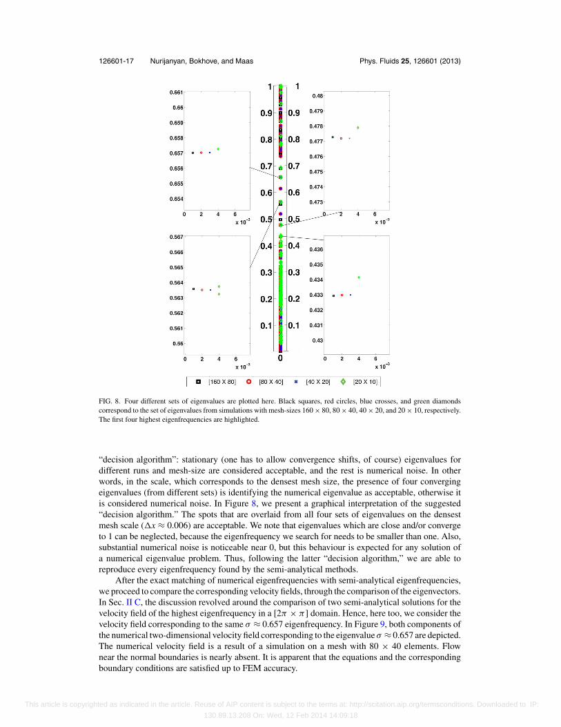
FIG. 8. Four different sets of eigenvalues are plotted here. Black squares, red circles, blue crosses, and green diamondscorrespond to the set of eigenvalues from simulations with mesh-sizes 160 × 80, 80 × 40, 40 × 20, and 20 × 10, respectively.The first four highest eigenfrequencies are highlighted.

“decision algorithm”: stationary (one has to allow convergence shifts, of course) eigenvalues fordifferent runs and mesh-size are considered acceptable, and the rest is numerical noise. In otherwords, in the scale, which corresponds to the densest mesh size, the presence of four convergingeigenvalues (from different sets) is identifying the numerical eigenvalue as acceptable, otherwise itis considered numerical noise. In Figure 8, we present a graphical interpretation of the suggested“decision algorithm.” The spots that are overlaid from all four sets of eigenvalues on the densestmesh scale (�x ≈ 0.006) are acceptable. We note that eigenvalues which are close and/or convergeto 1 can be neglected, because the eigenfrequency we search for needs to be smaller than one. Also,substantial numerical noise is noticeable near 0, but this behaviour is expected for any solution ofa numerical eigenvalue problem. Thus, following the latter “decision algorithm,” we are able toreproduce every eigenfrequency found by the semi-analytical methods.

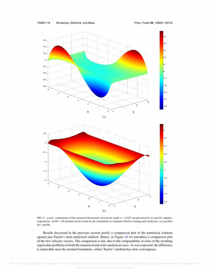
After the exact matching of numerical eigenfrequencies with semi-analytical eigenfrequencies,we proceed to compare the corresponding velocity fields, through the comparison of the eigenvectors.In Sec. II C, the discussion revolved around the comparison of two semi-analytical solutions for thevelocity field of the highest eigenfrequency in a [2π × π ] domain. Hence, here too, we consider thevelocity field corresponding to the same σ ≈ 0.657 eigenfrequency. In Figure 9, both components ofthe numerical two-dimensional velocity field corresponding to the eigenvalue σ ≈ 0.657 are depicted.The numerical velocity field is a result of a simulation on a mesh with 80 × 40 elements. Flownear the normal boundaries is nearly absent. It is apparent that the equations and the correspondingboundary conditions are satisfied up to FEM accuracy.

This article is copyrighted as indicated in the article. Reuse of AIP content is subject to the terms at: http://scitation.aip.org/termsconditions. Downloaded to IP:

130.89.13.208 On: Wed, 12 Feb 2014 14:09:18

126601-18 Nurijanyan, Bokhove, and Maas Phys. Fluids 25, 126601 (2013)

FIG. 9. u and v components of the numerical horizontal velocity for mode σ ≈ 0.657 are presented in (a) and (b) subplots,respectively. An 80 × 40-element mesh is used for the simulations in a domain which is rotating anti-clockwise. (a) u profile;(b) v profile.

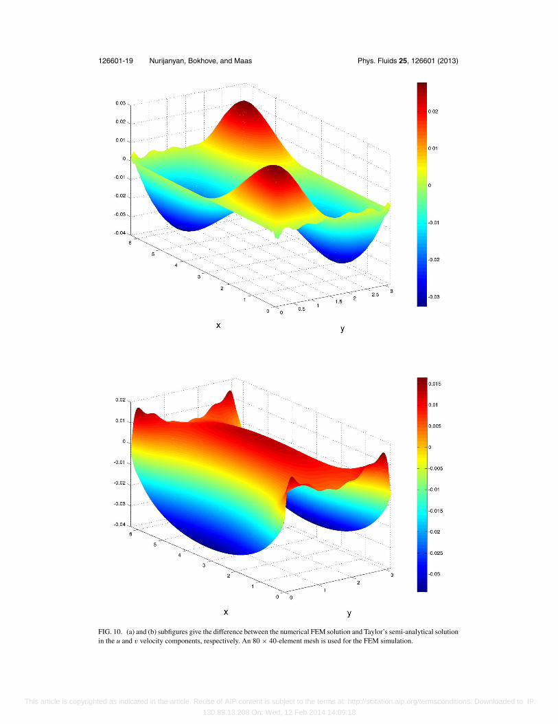
Results discussed in the previous section justify a comparison plot of the numerical solutionagainst just Taylor’s semi-analytical solution. Hence, in Figure 10 we introduce a comparison plotof the two velocity vectors. The comparison is fair, due to the comparability in sizes of the resultingeigenvalue problems in both the numerical and semi-analytical cases. As was expected, the differenceis noticeable near the normal boundaries, where Taylor’s method has slow convergence.

This article is copyrighted as indicated in the article. Reuse of AIP content is subject to the terms at: http://scitation.aip.org/termsconditions. Downloaded to IP:

130.89.13.208 On: Wed, 12 Feb 2014 14:09:18

126601-19 Nurijanyan, Bokhove, and Maas Phys. Fluids 25, 126601 (2013)

FIG. 10. (a) and (b) subfigures give the difference between the numerical FEM solution and Taylor’s semi-analytical solutionin the u and v velocity components, respectively. An 80 × 40-element mesh is used for the FEM simulation.

This article is copyrighted as indicated in the article. Reuse of AIP content is subject to the terms at: http://scitation.aip.org/termsconditions. Downloaded to IP:

130.89.13.208 On: Wed, 12 Feb 2014 14:09:18

126601-20 Nurijanyan, Bokhove, and Maas Phys. Fluids 25, 126601 (2013)

IV. SUMMARY AND CONCLUSIONS

We have shown numerically that the Proudman-Rao method for deriving modal solutions ofthe linear, rotating incompressible Euler equations in a (planar) rectangular parallelepiped boundedwith solid walls suffers from poor convergence in the interior of the fluid domain as well as a Gibbsphenomenon at the boundaries. Despite the concise structural construction, the solution is practicallyunusable. Therefore, an alternative mode decomposition solution (Taylor’s method) was presented.The three-dimensional problem was reduced to a two-dimensional problem by using the ansatz ofvertical modes in the z-direction, exactly repeating the arguments from Maas.8 By scaling the depthof the tank with H∗/nπ for the vertical mode n, we remove all references to the vertical and theproblem can be solved for each vertical mode strictly in the horizontal plane (whose size is fixedexcept for an n-dependent rescaling of the basin’s size). The resulting two-dimensional problem inthe horizontal plane was solved by employing ideas and results that Taylor1 used to determine therotational effects on long surface gravity waves. As in the Proudman-Rao method, Taylor’s methodalso leads to an infinite matrix eigenvalue problem, whose solution upon truncation gives similarresults. The novel mode solutions satisfy the linear Euler equations exactly, thus they are consideredto be an improvement over those obtained with the Proudman-Rao method. Nevertheless, the novelsemi-analytical solution has its own flaws. The mode solutions are, by construction, a superpositionof inertial analogs of surface Kelvin and Poincare wave solutions, which converge to solutions thatsatisfy the solid-wall boundary conditions. Unfortunately, the latter convergence is also slow. Bycontrast, the Proudman-Rao solution satisfies the no-normal flow boundary conditions exactly.

The latter motivated us to apply a continuous FEM discretisation to the reduced two-dimensionalproblem (based on using a standing wave in the vertical of the original three-dimensional problem) inorder to obtain numerical mode solutions that (weakly) satisfy no-normal flow boundary conditionsby construction. A modified FEM discretisation is proven to be symmetric and energy conserving on adiscrete level, which plays an essential role in the stability and accuracy of this scheme (e.g., Bokhoveand Johnson25). The resulting discrete system is solved via a generalised eigenvalue solver, whichunfortunately produces a substantial amount of numerical noise. Nevertheless, a simple “decisionalgorithm” is suggested to separate acceptable numerical eigenfrequencies from numerical noise.Finally, this numerical solution is tested against the semi-analytical solution.

Extensive comparison between the two semi-analytical and numerical solutions enables oneto adopt the most appropriate method for resolving the inertial waves. The Proudman-Rao methodfacilitates fast convergence of eigenfrequencies and the determination of semi-analytical solutionsthat satisfy the boundary conditions exactly because this is embedded in the construction algorithm.However, this method displays a Gibbs phenomenon at the boundaries. Unlike the Proudman-Rao method, Taylor’s method enables a semi-analytical solution exactly satisfying the governingequations in the interior, but with slow convergence near the boundaries. The numerical solution,based on a modified FEM discretisation, implements a very accurate but relatively slow method,which requires an extra step to separate the acceptable eigenfrequencies from numerical noise.Depending on one’s needs one might choose one of the suggested methods.

The solutions we have presented have been used to verify the novel numerical techniquedeveloped in Nurijanyan et al.26 for the initial-value problem of three-dimensional inertial waves inarbitrarily shaped domains. This method is geared to investigate whether wave attractors (Maas,9

Manders and Maas,23 and Rieutord et al.27) and complex eigenmodes (such as in Bokhove andAmbati28) emerge in domain shapes of sufficient geometric complexity.

Additionally, we note that solutions of the Euler equations, by default inviscid, presented aboveare also relevant in the viscous case (Navier-Stokes equations), which is not intuitive at first glance.In experiments like those in Fultz,10 McEwan,11 Manasseh,12, 13 Kobine,14 Thompson,15 Aldridgeand Toomre,16 Malkus,17 Vanyo et al.,18 Beardsley,19 Bewley et al.,20 Lamriben et al.,21 Boissonet al.,22 and Manders and Maas,23 a variety of forcing mechanisms and geometries have been applied.In some cases forcing occurs by pumping through viscous boundary layers, e.g., either on convex(outer) or concave (inner) parts of spherical shells; in other studies by means of the Euler force(using libration). Experiments performed in square domains (Bewley et al.,20 Lamriben et al.,21 andBoisson et al.22) seem to show that inviscid eigenmodes derived above are relevant in the sense that

This article is copyrighted as indicated in the article. Reuse of AIP content is subject to the terms at: http://scitation.aip.org/termsconditions. Downloaded to IP:

130.89.13.208 On: Wed, 12 Feb 2014 14:09:18

126601-21 Nurijanyan, Bokhove, and Maas Phys. Fluids 25, 126601 (2013)

energy spectra display peaks at inviscid eigenfrequencies of some of the larger scale eigenmodes.In two experiments (Bewley et al.20 and Lamriben et al.21) forcing arises by pulling a grid throughthe fluid, leaving a set of waves behind. In another experiment with a libration (Boisson et al.22),forcing occurs through Ekman-layer convergence, lending the spatial structure of the response muchmore of a beam-like character. Note, however, that due to the degeneracy discussed in Maas8 (near-degeneracy for numerical results) internal (gravity) and inertial waves have a much more flexible(“chameleonic”) spatial structure than that of the eigenmodes of elliptic problems (like surfacewaves). Indeed, in general one observes that the inviscid response (in combination with any spatialstructure in the forcing) is determining the field’s spatial structure, slaving the viscous (boundarylayer) response, and not the other way around.

ACKNOWLEDGMENTS

We would like to acknowledge the financial support of the Netherlands Foundation for TechnicalResearch (STW) for the project “A numerical wave tank for complex wave and current interactions.”

1 G. I. Taylor, “Tidal oscillations in gulfs and rectangular basins,” Proc. London Math. Soc. 20, 148–181 (1922).2 Lord Rayleigh, “Notes concerning tidal oscillations upon a rotating globe,” Proc. R. Soc. London 82(556), 448–464 (1909),

http://www.jstor.org/stable/92854.3 J. Proudman, “On the dynamic equation of the tides. Parts 1–3,” Proc. London Math. Soc., Ser. 2 18, 1–68 (1917).4 J. Proudman, “Note on the free tidal oscillations of a sea with slow rotation,” Proc. London Math. Soc. s2-35, 75–82 (1933).5 P. H. LeBlond and L. A. Mysak, Waves in the Ocean (Elsevier, Amsterdam, 1978).6 L. Kelvin, “Vibrations of a columnar vortex,” Philos. Mag. 10, 155–168 (1880).7 G. H. Bryan, “The waves on a rotating liquid spheroid of finite ellipticity,” Philos. Trans. R. Soc. London, Ser. A 180,

187–219 (1889).8 L. R. M. Maas, “On the amphidromic structure of inertial waves in a rectangular parallelepiped,” Fluid Dyn. Res. 33,

373–401 (2003).9 L. R. M. Maas, “Wave focussing and ensuing mean flow due to symmetry breaking in rotating fluids,” J. Fluid Mech. 437,

13–28 (2001).10 D. Fultz, “A note on overstability and the elastoid-inertia oscillations of Kelvin, Solberg and Bjerknes,” J. Meteorol. 16,

199–208 (1959).11 A. D. McEwan, “Inertial oscillations in a rotating fluid cylinder,” J. Fluid Mech. 40, 603–640 (1970).12 R. Manasseh, “Breakdown regimes of inertia waves in a precessing cylinder,” J. Fluid Mech. 243, 261–296 (1992).13 R. Manasseh, “Distortions of inertia waves in a rotating fluid cylinder forced near its fundamental mode resonance,” J.

Fluid Mech. 265, 345–370 (1994).14 J. J. Kobine, “Inertial wave dynamics in a rotating and precessing cylinder,” J. Fluid Mech. 303, 233–252 (1995).15 R. O. R. Y. Thompson, “A mechanism for angular momentum mixing,” Geophys. Astrophys. Fluid Dyn. 12, 221–234

(1979).16 K. D. Aldridge and A. Toomre, “Axisymmetric oscillations of a fluid in a rotating spherical container,” J. Fluid Mech. 37,

307–323 (1969).17 W. V. R. Malkus, “Precession of the earth as the cause of geomagnetism,” Science 160, 259–264 (1968).18 J. Vanyo, P. Wilde, P. Cardin, and P. Olson, “Experiments on precessing flows in the earth’s liquid core,” Geophys. J. Int.

121, 136–142 (1995).19 R. C. Beardsley, “An experimental study of inertial waves in a closed cone,” Stud. Appl. Math. 49, 187–196 (1970).20 G. P. Bewley, D. P. Lathrop, L. R. M. Maas, and K. R. Sreenivasan, “Inertial waves in rotating grid turbulence,” Phys.

Fluids 19, 071701 (2007).21 C. Lamriben, P. P. Cortet, F. Moisy, and L. R. M. Maas, “Excitation of inertial modes in a closed grid turbulence experiment

under rotation,” Phys. Fluids 23, 015102 (2011).22 J. Boisson, C. Lamriben, L. R. M. Maas, P. Cortet, and F. Moisy, “Inertial waves in rotating grid turbulence,” Phys. Fluids

24, 076602 (2012).23 A. M. M. Manders and L. R. M. Maas, “Observations of inertial waves in a rectangular basin with one sloping boundary,”

J. Fluid Mech. 493, 59–88 (2003).24 D. Rao, “Free gravitational oscillations in rotating rectangular basins,” J. Fluid Mech. 25, 523–555 (1966).25 O. Bokhove and E. Johnson, “Hybrid coastal and interior modes for two-dimensional flow in a cylindrical ocean,” J. Phys.

Oceanogr. 29, 93–118 (1999).26 S. Nurijanyan, J. van der Vegt, and O. Bokhove, “Hamiltonian discontinuous Galerkin FEM for linear, rotating incom-

pressible Euler equations: Inertial waves,” J. Comput. Phys. 241, 502–525 (2013).27 M. Rieutord, B. Georgeot, and L. Valdettaro, “Inertial waves in a rotating spherical shell: attractors and asymptotic

spectrum,” J. Fluid Mech. 435, 103–144 (2001).28 O. Bokhove and V. R. Ambati, “Hybrid Rossby-shelf modes in a laboratory ocean,” J. Phys. Oceanogr. 39(10), 2523–2542

(2009).

This article is copyrighted as indicated in the article. Reuse of AIP content is subject to the terms at: http://scitation.aip.org/termsconditions. Downloaded to IP:

130.89.13.208 On: Wed, 12 Feb 2014 14:09:18