A Novel Approach for Deterioration and Damage

Accepted in Journal of Structural Integrity and Maintenance

1

A Novel Approach for Deterioration and Damage Identification in Building

Structures Based on Stockwell-Transform and Deep Convolutional Neural

Network

Vahid Reza Gharehbaghia, Hashem Kalbkhanib, Ehsan Noroozinejad Farsangic*, T.Y. Yangd, Andy Nguyene,

Seyedali Mirjalilif,g & C. Málaga-Chuquitaypeh

a Research Scholar, Kharazmi University, Faculty of Civil Engineering, Tehran, Iran

([email protected]) b A/Professor, Department of Electrical Engineering, Urmia University of Technology, Urmia, Iran

(h.kalbkhaniuut.ac.ir) c A/Professor, Faculty of Civil and Surveying Engineering, Graduate University of Advanced Technology,

Kerman, Iran (*Corresponding Author: [email protected]) d Professor, The University of British Columbia, Vancouver, Canada ([email protected])

e A/Professor, University of Southern Queensland, Springfield Campus, Queensland 4030, Australia

([email protected]) f Center for Artificial Intelligence Research and Optimization, Torrens University Australia, Fortitude

Valley, Brisbane, QLD 4006, Australia ([email protected]) g Yonsei Frontier Lab, Yonsei University, Seoul, Korea

h A/Professor, Department of Civil and Environmental Engineering, Imperial College London, UK

([email protected])

Abstract

In this paper, a novel deterioration and damage identification procedure (DIP) is presented and applied to

building models. The challenge associated with applications on these types of structures is related to the

strong correlation of responses, which gets further complicated when coping with real ambient vibrations

with high levels of noise. Thus, a DIP is designed utilizing low-cost ambient vibrations to analyze the

acceleration responses using the Stockwell transform (ST) to generate spectrograms. Subsequently, the ST

outputs become the input of two series of Convolutional Neural Networks (CNNs) established for

identifying deterioration and damage to the building models. To the best of our knowledge, this is the first

time that both damage and deterioration are evaluated on building models through a combination of ST and

CNN with high accuracy.

Keywords: Deterioration, Damage, Stockwell Transform, Convolutional Neural Networks (CNNs), Deep

Learning


2

Introduction and Motivations

The accumulation of deterioration in structures during their lifetime leads to the reduction of

strength and performance and imperils their serviceability and safety (Monavari, 2019).

Subsequently, the capability of a structure to endure extreme incidents diminishes over time.

Hence, preserving the functionality of structures and enhancing their performance level to reduce

upkeep costs have become a central focus in structural health monitoring (SHM). It is noteworthy

that embedding an SHM system in the structure makes it possible to continuously monitor the

system's changes during operation time. This potential allows determining the appropriate moment

for essential or preventive maintenance action (EMA and PMA) and thereby reduces the risk level

of probable breakdowns (Figure 1).

Figure 1. Effect of maintenance actions on structure [adapted from (Berkowski & Kosior-Kazberuk, 2017)]

Based on a survey conducted on 225 building cases in the USA, it has been demonstrated that

deterioration is a frequent concern deserving attention (Wardhana & Hadipriono, 2003). Therefore,

identifying structures' responses to detect variations is supposed to be a significant task that can

ensure safety and related financial considerations.

Damage and deterioration are defined as degradation in a system's performance due to changes

in material, components, or structure connections. However, compared to damage, deterioration

identification requires more accurate and reliable techniques (Monavari, 2019). Recently, several

studies have focused on damage identification through variations in the structure responses.


3

Nonetheless, while these surveys have illuminated numerous practical approaches in the sense of

identification and localization of damage on simple components or bridges (Gillich et al., 2017;

Sha et al., 2020) (Jayasundara et al., 2020), fewer have been done to assess slight damages on

building structures (Regier & Hoult, 2015). This concern is exacerbated in complex structures like

buildings, where a strong correlation of responses is considered one of the challenging issues

(Gharehbaghi et al., 2020). Deterioration recognition in complex systems requires laborious efforts

since not only ambient excitations lead to lower amplitudes in responses, but also noise and

operational effects influence the performance of detection.

For the sake of illustration, in Figure 2, two samples of signals corresponding to a damaged

and deteriorated state are plotted versus the baseline or healthy state. The signals are captured from

two building specimens with distinct deterioration and damage scenarios discussed in the

following sections. As can be seen, the deterioration signal is hardly distinguished from the healthy

signal. By contrast, the signal of damage reveals significant variations compared to the baseline

state and thereby is readily apparent even to the naked eye.

(a) Signal of damage vs. baseline (b) Signal of deterioration vs. baseline

Figure 2. Comparison of deterioration and damage signals

There are two main approaches to conduct SHM in practice, including model-based and data-

driven SHM. In the first technique, a complicated model of the monitored system is needed, which

requires information regarding geometry, materials, and boundary conditions of the structure. In

the former, however, the real data collected from sensors embedded in the structure is deployed to

recognize various system conditions. Stochastic methods coupled with signal processing


4

techniques are the principal tools for disclosing hidden features within the responses in the realm

of data-driven SHM. Herein, for the sake of pattern recognition, machine learning algorithms are

prevalent, including classical machine learning algorithms such as decision trees, Support vector

machines (SVMs), and K nearest neighborhoods (KNNs) or deep learning approaches.

According to the above limitations and motivations, this article attempts to establish a system

for deterioration assessment in a building based on a data-driven strategy and deep learning for

pattern recognition as one of the most promising trends in Artificial intelligence. The rest of the

paper is organized as follows.

First, some of the data-driven studies with an emphasis on deterioration detection are presented.

Next, deep learning basics are introduced, and relevant investigations are reviewed. Third, the

deterioration identification procedure (DIP) is illustrated in sequential steps. Fourth, the specimens

for the deterioration and damage study are depicted. Last, the DIP is applied to the case studies,

and the results are discussed.

A review on deterioration detection in building structures

Signal processing, stochastic methods, and machine learning algorithms play a significant role in

extracting features, developing damage indices, and pattern recognition in data-driven SHM. Time

series, Fourier transformation, wavelets, Wigner-Ville distribution (WVD), empirical mode

decomposition (EMD), and Stockwell transform are some of the signal processing used frequently

by researchers. Herein, some studies that attempted to identify slight damages on building

structures are reviewed.

Santos et al. (Santos et al., 2016) were successful in detecting damages on a real bridge using

unsupervised machine learning methods. To this end, Neural Networks were adopted for structural

estimation response, and clustering techniques were applied for classifying the neural network

estimation errors. A moving windows process method was utilized for enduring the continuous

online procedure. Consequently, small reductions in single cables' stiffness were detected using a

small number of inexpensive sensors.

Wang et al. (Wang et al., 2016) deployed the Autoregressive (AR) time series coefficients for

detecting slight damages on a cantilever beam and a building SHM benchmark. It was deducted

that the control charts had the potential to identify damage in the early stages, even in a noisy


5

environment. However, the precise location and severity of damage could not be indicated based

on that study.

Monavari et al. (Monavari et al., 2018) developed a signal-based approach utilizing residuals

of AR time-series. The potential of time series for analyzing ambient vibrations and their

sensitivity and reliability compared to other vibration-based damage detection was the primary

motive. In this study, a novel model order estimation algorithm was established to fit structural

responses with more than 95% accuracy. Eventually, the statistical hypotheses of a two-sample f-

test were applied to the AR model's residuals as a deterioration indicator. The efficiency of the

proposed methodology was validated by detecting multiple deterioration locations on two multi-

story RC frames in a noisy environment.

A robust model-based technique based on long-term monitoring data was proposed by Nguyen

et al. (Nguyen et al., 2019). To build an empirical model of the complex structure, operational

modal analysis (OMA) is used coupled with an initial FEM of the structure made by as-built

drawings. In this paper, a hybrid model updating procedure was exploited, coupled with sensitivity

analysis. The gradual, subtle area-section reduction was considered as the simulation of slight

damage in life-cycle assessment. Subsequently, the authors efficiently predicted the deterioration

mechanism under serviceability loading in a real existing case study of a 10-story benchmark

structure.

Gharehbaghi et al. (Gharehbaghi et al., 2020) established a novel algorithm to select sensitive

uncorrelated features derived from AR models and statistical indices. The selected features were

then used for generating a stochastic pattern for each state in the system. A linear discriminant

classifier was applied to the pattern for separating damage and deterioration conditions in two

building models. It was shown that the proposed strategy had the potential for classifying different

states of structure even in a noisy environment.

In another paper, Gharehbaghi et al. (Gharehbaghi et al., 2021) utilized time-frequency processing

using wavelets coupled with some statistical insides for extracting features of damage and

deterioration in specimens. A novel feature selection method extracted sensitive features based on

baseline signals which built structural behavior patterns. Classical machine learning algorithms

including ANN, SVM, and KNN were deployed for discriminating healthy and unknown status

within building models. The efficiency of the proposed technique was verified under various

conditions such as signal length, sampling rate, and the number of features. It was proven that the


6

method could detect, locate, and assess the severity of damage and deterioration under

environmental variabilities such as high noise and operational effects.

Deep learning fundamentals

In real-world intelligence applications, many factors and variations exist in the data. Extracting

high-level and abstract features, such as detecting specific objects in a picture or finding individual

pixels in a color image, is challenging. Many of these factors of variation require a cutting-edge,

nearly human-level knowledge of the data. Deep learning addresses this issue in representation

learning by decomposing a complex problem into more straightforward representations. This

matter allows a computer to develop sophisticated models from simple concepts (Heaton, 2018).

For instance, a deep leading algorithm can understand complex features for detecting unique

objects within a picture using corners and contours of pixels.

A central feature of AI is the use of various Artificial Neural Networks along with some

connected layers. It shares similar algorithms with Machine Learning, including four stages in

terms of building a paradigm. Deep Learning is different from Neural Networks in some aspects,

as demonstrated in Figure 3. As seen, the feature extraction and classification are conducted within

a more complicated neural network. Notably, deep neural networks reveal higher accuracy and

efficiency in big data than classical machine learning algorithms due to the high complexity of

structure (LeCun et al., 2015).

Concerning configuration, deep neural networks are known via four major architectures,

namely Unsupervised Pre-trained Networks (UPNs), Convolutional Neural Networks (CNNs),

Recurrent Neural Networks, and Recursive Neural Networks (RNNs) (Patterson & Gibson, 2017).

In brief, a UPN manages and also learns the input data in the network by itself. It weighs the first

layer through unsupervised pre-trained data. Recurrent Neural Networks and RNNs are exploited

to process time-sequential data. In this category, Long short-term memory (LSTM) (Luo et al.,

2018) is one of the popular recurrent neural networks used for predicting the time sequences over

time (Deng et al., 2020).


7

Figure 3. Machine Learning vs. Deep Learning

Compared to other types of networks, CNNs have been widely used in data science, especially

for addressing image classification problems since they can learn directly from the raw images.

They are used to extract the multi-scale localized spatial features from the input image by

performing local filtering of the input image (Toh & Park, 2020).

CNNs consist of different layers, including convolution, rectified linear unit (ReLU), pooling,

fully connected layers, and softmax, as shown in Figure 4. The first layer obtains high-level

features from a part of the data using small kernels. For the sake of fast training and having lower

sensitivity to initialization, the convolution's output is usually normalized using mini-batches.

The ReLU is a nonlinear activation function generating new outputs as follows:

max{0, }out inx x (1)

where inx depicts the output elements of the batch normalization layer and outx shows the output

of the ReLU layer. Downsampling is implemented on the output feature map of the ReLU layer.

Herein, max pooling is the most common pooling operation that uses the maximum value of a

neighborhood area in the feature map. Additionally, in order to avoid overfitting errors, the dropout

layer is used. In this layer, each neuron may be eliminated in a particular repetition of the training

stage with the probability of p . Notably, this layer is just employed in the training stage and is


8

not used in validation or testing. Subsequently, the fully connected and softmax layer can classify

the input data for identification purposes.

Figure 4. Typical architecture of CNN (Patterson & Gibson, 2017)

In general, a combination of SHM and deep learning can be investigated through two central

frameworks. Image-based Deep SHM (ID-SHM) employs images as input, and Signal-based Deep

SHM (SD-SHM) utilizing signals or one-dimensional data. Following the first framework, as the

most common type, deep learning is employed instead of human sight to classify and analyze

collections of raw images.

It is essential to note that sufficient numbers of images should be collected via various kinds

of hardware as well as pieces of equipment, including digital cameras, infrared cameras, robotic

systems, and Digital Image Correlation (DIC) systems. In light of this framework, multiple image

processing operations are conducted to obtain information from images. This information is then

employed as the input features of a deep learning network.

Regarding ID-SHM, Zhang et al. (Zhang et al., 2016) proposed a deep learn-based method for

crack detection in pavements using a data set of 500 images captured with a smartphone camera.

They trained the network through the Stochastic Gradient Descent (SGD) method accelerated by

GPU rather than ReLU as the activation function. SVM and the Boosting algorithms were

compared with the proposed method. As a result, it was shown that CNN had higher performance

in classifying crack patches from the background.

Kim et al. (Kim et al., 2019) established a novel method for locating cracks on concrete surfaces

in noisy patterns. In that study, image binarization was put to use to extract cracked regions coupled


9

with a CNN for classification. The classification models were built based on speeded-up robust

features (SURF) and CNN. It was concluded that the overall performance of the CNN method was

better than the SURF-based method in the majority of cases. Moreover, combining deep neural

networks with SVM classifiers with local/global features could enhance the accuracy compared to

separate deployment of each method.

Li et al. (Li et al., 2020) studied automatic crack inspection within a tunnel. Accordingly, U-

Net and a CNN were combined and an updated version of the clique (CliqueNet) was used to

distinguish cracks from backgrounds using digital camera images. A total of 200 manually labeled

images at a pixel level were used for the training and testing. The proposed approach was simple

but effective, showing success in detecting internal cracks with high accuracy.

On the other hand, SD-SHM methods use structure responses (accelerations, displacements,

velocities, and strains) to detect an anomaly. Based on that, signal processing techniques, namely

time-series, Fourier transform (FT), Short-time Fourier transform (STFT), Wavelet Transform

(WT), Stockwell transform (ST), and Empirical mode decomposition (EMD) are utilized to

analyze the responses. By applying these operations to the recorded signal, numerous attributes

within specific domains (time, frequency, or time-frequency) are extracted as sensitive features

that can reflect changes in the structure.

In earlier approaches, conventional classifiers like SVM, Principal Component Analysis (PCA),

and Artificial Neural Network (ANN) were employed to pre-process and classify data.

Nonetheless, in SD-SHM, researchers benefit from promising deep learning networks as a

powerful tool along with signal processing techniques. For example, Abdeljaber et al. (Abdeljaber

et al., 2017) established an adaptive CNN that could detect different damage scenarios on a large-

scale building model using acceleration measurements. Damages were simulated by loosening the

bolts at the joint. Moreover, 31 damage scenarios were utilized for training the network. It was

shown that the method could locate single and double damage cases in real-time.

Avci et al. (Avci et al., 2018) exploited the methodology proposed in (Abdeljaber et al., 2017)

with a shallow structure, but this time with the aid of triaxial accelerations measured with a

wireless sensor network (WSN). The authors attempted to find the most sensitive axis for detecting

damage. Their results demonstrated that the modified approach was promising in terms of the

location of damage under ambient vibrations.


10

Sarawgi et al. (Sarawgi et al., 2019) introduced an experimental procedure that was capable of

detecting damage on an I-AISC benchmark structure through 4 phases with the aid of a CNN. It

was shown that the proposed approach was capable of detecting and localizing damage in the

laboratory model. Further studies regarding the application of CNN in SHM are reviewed in this

reference (Avci et al., 2020).

The above review indicates that deep learning has become a popular tool for damage

identification. However, its potential has not been explored and harnessed enough in the case of

deterioration. In light of this, the authors present an intelligent system for deterioration

identification in building structures.

Case Studies

In this section, the case studies are presented in details.

First Case-Study: Deterioration Model

In this paper, a full-scale finite element model (FEM) of a three-story reinforced concrete (RC)

frame, which has been modeled in the IDARC program (Reinhorn et al., 2006), is used to confirm

the efficiency of the proposed method. The height of each story and the bay width is 3000(mm)

and 4000(mm), respectively. The element sections of the model are shown in Figure 5.


11

Figure 5. Three-story RC frame (Monavari et al., 2018)

Notably, this model was previously used for deterioration identification using a time-series and

wavelet approach (Gharehbaghi et al., 2021; Gharehbaghi et al., 2020; Monavari et al., 2018). The

input excitations were obtained from a real-world site under ambient environmental vibrations

with a sampling rate of 200 Hz. The real site corresponds to the location of the P-block building

at the Gardens Point campus of QUT, Australia. Since the input excitations are recorded from a

real building site, they consist of a high noise level, human activities, traffic vibrations, and other

environmental forces (Monavari, 2019).

In this case study, deterioration is defined as a continuous loss of cross-section. The structure

was monitored for a 50-year period and comprising five states of intensity. During these states,

the cross-section area of the left column's bars gradually reduced, and the annual deterioration rate

(ADR) for the cross-section area was considered equal to 2×10-3. The first state indicates the

baseline (State 1), and the four following states are the deteriorated conditions starting from slight

deterioration (State 2) to significant deterioration (State 5).

The deterioration modeling scenarios for the three cases are introduced in Table 1.

Consequently, the deterioration rate (DR) for a year can be computed by multiplying the duration

of deterioration (DOD) process and the ADR (Monavari et al., 2018).

Reduced cross - section area

1Refrenced cross - sectionarea

ADR year (2)

Table 1. Deterioration scenarios (Monavari et al., 2018)

Scenario Story 1 Story 2 Story 3

1 Deteriorated None None

2 None Deteriorated None

3 None None Deteriorated

Second Case-Study: Damage Model


12

Regarding the damage model, an SHM benchmark is presented here. This model is a three-story

bookshelf with metal columns and aluminum floor plates, as shown in Figure 6. Moreover, four

isolators allow the structure to sway in horizontal directions with the aid of a hydraulic shaker. The

structure is instrumented by piezoelectric single-axis accelerometers. There are nine structural

state conditions. The first state indicates the healthy state, and the rest are related to damage

conditions. Damage and environmental changes were simulating by stiffness reduction of columns

and replacing a mass, respectively. The healthy condition was considered with no stiffness

reduction in sections and no mass on floors. For applying a damage scenario, columns were

replaced by another section with a smaller section-area. A total of 450 records (nine states, each

of which has 50 records) with a sampling rate of 320 Hz are recorded in each state, as shown in

Table 2.

Table 2. Data labels of structural states (T. Nguyen et al., 014)

Label Record Details Description

State 1 0-50 No mass and no stiffness reduction Healthy

State 2 51-100 Mass = 1.2 kg at the base Environmental effects

State 3 101-150 Mass = 1.2 kg on the 1st floor Environmental effects

State 4 151-200 87.5% stiffness reduction in column 1BD Damaged

State 5 201-250 87.5% stiffness reduction in column

1AD and 1BD Damaged



2AD and 2BD Damaged



3AD and 3BD Damaged


13

Figure 6. Three-story bookshelf [adapted from (Gharehbaghi et al., 2021)]

Deterioration Identification Procedure (DIP)

Figure 7 presents the DIP procedure proposed. As shown, the proposed strategy is performed on

the building dataset in three sequential steps, including pre-processing, processing in the time-

frequency domain, and classification using CNN, which are explained in detail in the following

sections.


14

Figure 7. DIP diagram

Step1: Pre-processing

First, the high-frequency noise of the responses (story accelerations) is removed by employing a

12-order low-pass Chebyshev filter. This filter is selected because of the fast speed of denoising.

More details about this filter can be found in (Vaseghi, 2008).

Next, mathematical and statistical operations are conducted on the data in order to reduce the

effects of environmental and operational effects. Let ix and ix be the measured and standardized

signals; hence, the data normalization is carried out as follows (Monavari et al., 2018):

ˆ iix x

x (3)

where x and show the mean and standard deviation of the measured signal.

Typically, in a building dataset, the responses of stories are correlated; hence, it is essential to

conduct some operations for decorrelating or whitening. In this study, Zero-Phase Component

Analysis (ZCA) is utilized to remove the cross-correlation between signals (Gharehbaghi et al.,

2020). Afterward, the pre-processed signals are used in the next step in the time-frequency

analysis.

Step 2: Processing in Time-Frequency domain

Several methods have been proposed and used for time-frequency analysis. Stockwell Transform

(ST), introduced by Stockwell in 1996 (Kalbkhani & Shayesteh, 2017), shares similarities with

STFT, and both techniques can reveal the time distribution of various frequency bands. Since

STFT inherits a fixed window width, it cannot be implemented primarily for non-stationary

signals.

By contrast, ST benefits from a flexible window as a frequency function, inheriting the benefits

of the multi-resolution decomposition like continuous wavelet transform (CWT). Thus, while

having higher frequency bands, it provides efficient processing capabilities with a fine-scaled

window generating fine resolution and coarse resolution low frequencies (Kalbkhani & Shayesteh,


15

2017). Notably, ST can be presented using CWT and a phase factor. In this regard, the CWT of

( )x t is formulated as follows:

( ) ( , )( , ) x t w t d dtW d (4)

where and d denote the location of the window at time axis and dilation term, respectively, and

( , )w t d is the mother wavelet defined as:

2 2

22( , )2

f tj ft

fw t f e e (5)

In the above, f shows the frequency in Hz, which is inverse of ( 1/ )d f d and 1j .

Accordingly, by multiplying the phase factor, the one-dimensional continuous ST of ( )x t is:

2( , ) ( , ) j fS f W d e (6)

Alternatively, by substituting (4), ST can also be written as follows (Sartipi et al., 2020):

2 2( )

2 2( )( , )2

t fj ftx t e

fS f e dt (7)

Regarding (6) and (7), it is apparent that the window length varies. It means that, at low

frequencies, the window becomes more expansive, while at high frequencies, it becomes narrower.

Thus, ST is capable of providing a proper resolution within the various frequency bands of

structural responses (Ghasemzadeh et al., 2018).

Moreover, ST has some merits compared to other transformations since (Stockwell, 2007):

It can combine frequency-dependent resolution with an absolute reference phase.

It measures the local amplitude spectrum coupled with the local phase spectrum, while WT

provides local amplitude/power spectrum.

Contrary to most of the WT approaches, ST can be implemented on complex time series.

Significantly, ST has been used mainly for medical diagnosis, including Magnetic resonance

imaging (MRI) and electroencephalography (EEG) signals, and relatively few studies have been

done in the realm of structural damage identification (Kalbkhani & Shayesteh, 2017; Sartipi et al.,

2020). Accordingly, this study attempts to employ ST to identify building structures for the first

time.


16

Step3: Classification

Similar to CWT and according to Eq. (7), the output of ST is complex-valued. Therefore, after

analyzing each record of signals, a series of complex matrices are obtained. Considering the ST

matrices, each from the record of one sensor, we have multi-dimensional features that can be

represented in the form of spectrograms that are utilized as the input of robust CNNs. According

to Figure 5, two types of CNNs are designed in this paper; one for localization and the other for

assessing damage severity. First, a CNN is utilized on the colored images to detect the correct story

level. Second, three distinctive CNNs classify different deterioration or damage scenarios.

Five-fold cross-validation is adopted for training and testing of CNNs in all classification

problems. To this end, the available data is partitioned into five non-overlapping parts, and the

training and testing procedure is repeated five times, and the results are then averaged. In each

trial, four parts are used for training, and the remaining one is used for testing. The set of

parameters used in the training process of CNNs are given in Table 3.

Table 3. Parameters used in the training process

Parameter Value

Optimizer Stochastic gradient descent with momentum (SGDM)

Loss function Cross-entropy

Momentum 0.9

Batch size 32

Maximum number of epochs 200

Learning Rate 0.002

Regularization parameter 0.001

Learning rate drop factor 0.1

Learning rate drop period 20

Regarding the first case study and considering one sensor in each story, the input of localization

CNN has a size of 256x1024x3. This model consists of 22 layers. It has three layers from each of

convolution, batch normalization, max pooling, and fully connected layers. Also, there are five

ReLU layers, two dropout layers, one softmax, and some classification layers. It should be


17

mentioned that dropout layers are only used in the training process and are not involved in the test

phase.

After locating the deteriorated story, the severity of deterioration is recognized using a different

CNN. The CNN structure has three layers from each of the convolution, batch normalization, and

max-pooling layers. Also, there are four ReLU layers, two fully connected layers, and one layer

from each of the dropouts, softmax, and classification layers.

Regarding the second case study, a CNN with 20 layers is designed for localization of damage.

After locating the damaged story, the severity is assessed using three distinctive CNNs designed

for each story.

Results and Discussion

In this section, the results and discussion on all case studies are given.

First Case Study (Deterioration)

In the first case study, 1024 samples from deterioration signals are considered; as a result, the ST

of the sensor record is a 513×1024 complex-valued matrix, and its absolute is utilized for the

classification. There are three 513×1024 matrices for three sensors that can be depicted as colored

images. The output of ST shows that there is no information in frequencies higher than 25 Hz in

the deterioration signals since they are removed for the sake of better representation as well as

reducing computational complexity. The ST of the healthy state and some of the deteriorated

scenarios are depicted in Figure 8.

(a) Healthy (b) Scenario 1, Level 1


18

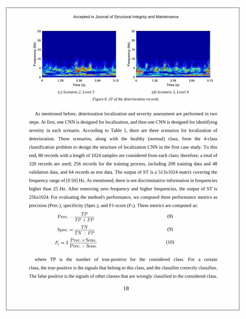
(c) Scenario 2, Level 3 (d) Scenario 3, Level 4

Figure 8. ST of the deterioration records.

As mentioned before, deterioration localization and severity assessment are performed in two

steps. At first, one CNN is designed for localization, and then one CNN is designed for identifying

severity in each scenario. According to Table 1, there are three scenarios for localization of

deterioration. These scenarios, along with the healthy (normal) class, form the 4-class

classification problem to design the structure of localization CNN in the first case study. To this

end, 80 records with a length of 1024 samples are considered from each class; therefore, a total of

320 records are used; 256 records for the training process, including 208 training data and 48

validation data, and 64 records as test data. The output of ST is a 513x1024 matrix covering the

frequency range of [0 50] Hz. As mentioned, there is not discriminative information in frequencies

higher than 25 Hz. After removing zero frequency and higher frequencies, the output of ST is

256x1024. For evaluating the method's performance, we computed three performance metrics as

precision (Prec.), specificity (Spec.), and F1-score (F1). These metrics are computed as:

Prec. TPTP FP

(8)

Spec. TNTN FP

(9)

1Prec. Sens.2Prec. Sens.

F (10)

where TP is the number of true-positive for the considered class. For a certain

class, the true-positive is the signals that belong to this class, and the classifier correctly classifies.

The false positive is the signals of other classes that are wrongly classified to the considered class.


19

TN is the true-negative, which is the number of signals that do not belong to the considered class,

and the classifier does not classify them to the considered class. Also, Sens. is the sensitivity (or

recall) which is computed as:

Sen. TPTP FN

(11)

where FN is the number of false-negative predictions for the considered class, the false-negative

is the signals that belong to the considered class, while the classifier is wrongly classified into

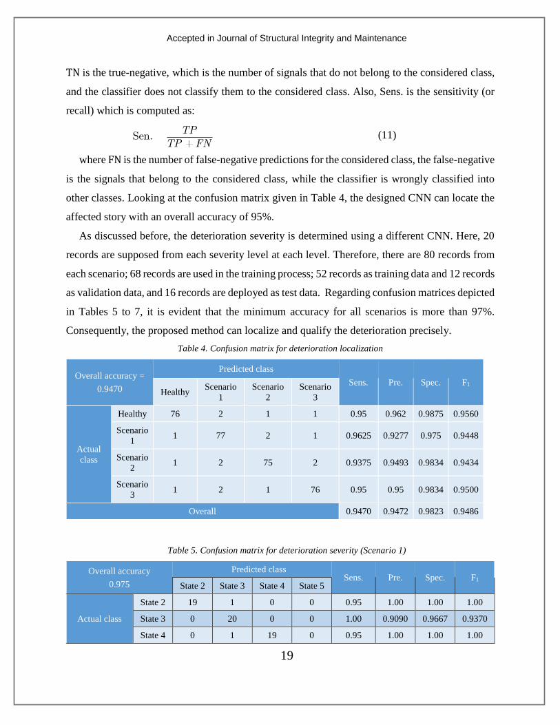
other classes. Looking at the confusion matrix given in Table 4, the designed CNN can locate the

affected story with an overall accuracy of 95%.

As discussed before, the deterioration severity is determined using a different CNN. Here, 20

records are supposed from each severity level at each level. Therefore, there are 80 records from

each scenario; 68 records are used in the training process; 52 records as training data and 12 records

as validation data, and 16 records are deployed as test data. Regarding confusion matrices depicted

in Tables 5 to 7, it is evident that the minimum accuracy for all scenarios is more than 97%.

Consequently, the proposed method can localize and qualify the deterioration precisely.

Table 4. Confusion matrix for deterioration localization

Overall accuracy =

0.9470

Predicted class

Sens. Pre. Spec. F1 Healthy

Scenario

1

Scenario

2

Scenario

3

Actual

class

Healthy 76 2 1 1 0.95 0.962 0.9875 0.9560

Scenario

1 1 77 2 1 0.9625 0.9277 0.975 0.9448

Scenario

2 1 2 75 2 0.9375 0.9493 0.9834 0.9434

Scenario

3 1 2 1 76 0.95 0.95 0.9834 0.9500

Overall 0.9470 0.9472 0.9823 0.9486

Table 5. Confusion matrix for deterioration severity (Scenario 1)

Overall accuracy

0.975

Predicted class Sens. Pre. Spec. F1

State 2 State 3 State 4 State 5

Actual class

State 2 19 1 0 0 0.95 1.00 1.00 1.00

State 3 0 20 0 0 1.00 0.9090 0.9667 0.9370

State 4 0 1 19 0 0.95 1.00 1.00 1.00


20

State 5 0 0 0 20 1.00 1.00 1.00 1.00

Overall 0.975 0.9772 0.9917 0.9843


Overall accuracy =

0.9875



Actual class

State 2 20 0 0 0 1.00 1.00 1.00 1.00

State 3 0 19 1 0 0.95 1.00 1.00 0.9744

State 4 0 0 20 0 1.00 0.9524 0.9833 0.9756

State 5 0 0 0 20 1.00 1.00 1.00 1.00

Overall 0.9875 0.9881 0.9958 0.9875


Overall accuracy =

0.975



Actual class

State 2 20 0 0 0 1.00 1.00 1.00 1.00

State 3 0 20 0 0 1.00 0.9524 0.9833 0.9756

State 4 0 1 19 0 0.95 0.95 0.9833 0.9500

State 5 0 0 1 19 0.95 1.00 1.00 0.9744

Overall 0.975 0.9756 0.9916 0.975

Second Case Study (Damage)

Like the first case, 1024 samples from each record are considered to obtain the ST of damage

signals. The results showed that there is not much useful information on frequencies above 80 Hz.

Hence, they have been omitted for better representation and to reduce computational complexity.

The ST of different states in the second case study is given in Figure 9.


21

(a) State 1 (b) State 2 (c) State 3

(d) State 4 (e) State 5 (f) State 6

(g) State 7 (h) State 8 (i) State 9

Fig. 9. ST of the damage records.

A look through the ST of signals (Figures 8 and 9) discloses that the dominant frequency of

damage sate is roughly 20 Hz, four times the deterioration with the frequency of 5 Hz. It should

be noted that damage signals experience further fluctuations. Additionally, the damage signals

have higher amplitudes since they are plotted with brighter colors coupled with higher contrast

than the deterioration state.


22

Regarding the damage case, the same steps are taken, as illustrated for the deterioration case.

Thus, according to Table 2, there are three scenarios for damage localization plus one healthy case.

As a result, there are four classes in the classification problem.

As in the preceding case, 80 records with 1024 samples are considered for each class. A total

of 320 records are used; 256 records for the training process, including 208 training data and 48

validation data, and 64 records for testing. The ST output is a 513x0124 matrix, including the

frequency range of [0 80] Hz. Finally, after removing zero frequency and higher frequencies, the

output of ST is 256x1024.

Conclusively, Table 8 denotes that the methodology's overall accuracy in locating damaged

stories is roughly 96.0 percent. Eventually, as shown in confusion matrices (Tables 9-11), a

minimum accuracy of about 97.0 percent is achieved by deploying the DIP on the damage case.

In the last section, the obtained results are compared with a similar work conducted by

Gharehbaghi et al. (Gharehbaghi et al., 2021) named REF in this paper. In REF, the wavelet is

used for signal processing in the time-frequency domain, and conventional machine learning

algorithms are chosen for classification. To have a rational comparison, the accuracy in

localization and severity determination are defined with an average index of both. For instance,

regarding the first case study, in scenario 1, the overall accuracies for locating deteriorated story

and severity assessments are 0.95 and 0.975, respectively. Therefore, the average accuracy is equal

to 0.9625. The same procedure is conducted for calculating average accuracies in the REF. In

Figure 10, the results for both methodologies are compared. It is evident that the DIP method has

enhanced the performance of classification, especially for the second scenario, and the minimum

accuracy of roughly 96% has been achieved in this paper.

Table 8. Confusion matrix for damage localization

Overall accuracy =

0.982

Predicted class Sens

. Prec.

Spec

. F1

Health

y

Stor

y 1

Stor

y 2

Stor

y 3

Actua

l class

Health

y 47 3 0 0 0.94

0.95

9

0.99

6

0.94

9

Story 1 2 198 0 0 0.99 0.97

1

0.97

6 0.98

Story 2 0 1 99 0 0.99 1 1 0.99

5


23

Story 3 0 2 0 98 0.98 1 1 0.98

9

Overall 0.98

2

0.98

2

0.98

9

0.98

2

Table 9. Confusion matrix for damage severity (Story 1)

Overall accuracy

= 0.97

Predicted class

Sens. Prec. Spec. F1

State

2

State

3

State

4

State

5

Actua

l class

Stat

e 2 49 1 0 0 0.98 0.961 0.987 0.973

Stat

e 3 2 48 0 0 0.96 0.979 0.993 0.986

Stat

e 4 0 0 48 2 0.96 0.979 0.993 0.986

Stat

e 5 0 0 1 49 0.98 0.961 0.986 0.973

Overall 0.97 0.97 0.989 0.979


Overall accuracy = 0.99

Predicted class


State 6 State 7

Actual

class

State 6 49 1 0.98 1 1 1

State 7 0 50 1 0.98 0.98 0.98

Overall 0.99 0.99 0.99 0.99


Overall accuracy = 0.98

Predicted class


Sate 8 Sate 9

Actual

class

Sate 8 49 1 0.98 0.98 0.98 0.98

Sate 9 1 49 0.98 0.98 0.98 0.98

Overall 0.98 0.98 0.98 0.98


24

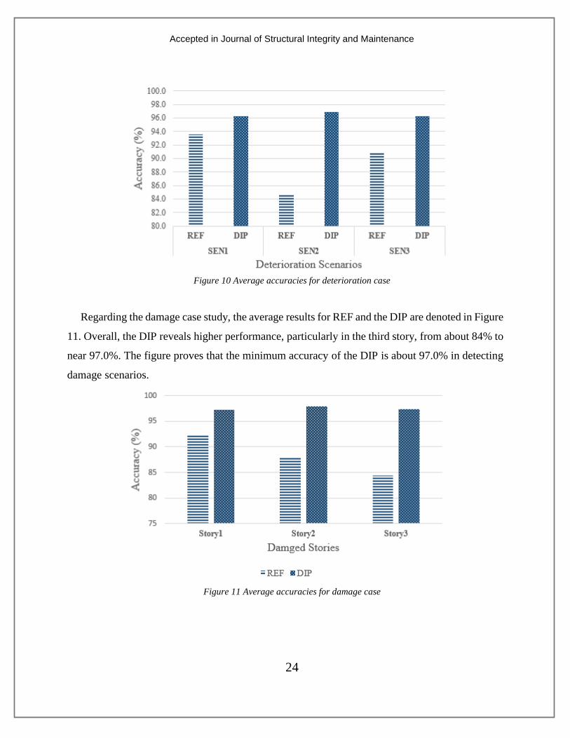
Figure 10 Average accuracies for deterioration case

Regarding the damage case study, the average results for REF and the DIP are denoted in Figure

11. Overall, the DIP reveals higher performance, particularly in the third story, from about 84% to

near 97.0%. The figure proves that the minimum accuracy of the DIP is about 97.0% in detecting

damage scenarios.

Figure 11 Average accuracies for damage case


25

Conclusion

In this article, a novel methodology was presented using a data-driven approach capable of

detecting deterioration and damage through output acceleration responses. To the best of the

authors' knowledge, this is the first-ever development of a procedure that can detect both

deterioration and damage via an innovative combination of Stockwell Transform (ST) and

Convolutional Neural Networks (CNN). In this respect, an ST is applied to obtain complex

matrices expressed as high dimensionality images representing various frequency bands in the

time-frequency domain. After pre-processing the acceleration input, a CNN is employed to locate

the affected story regarding the DIP. Afterward, another CNN is used to qualify damage and

deterioration in each story. Notably, the established DIP successfully detected deterioration and

damage in both models with high accuracy. Due to the flexibility of DIP, this procedure can also

be utilized for various types of structures such as bridges or dams, along with various types of

damage scenarios broadening the impact of this study. However, although the DIP has efficient

performance regarding damage and deterioration detection under ambient and forced vibration

with high accuracy, using separate CNNs for each story translates into high computational time to

train the network. Thus, the authors are looking forward to establishing and enhancing DIP

procedures that use only a CNN regardless of the number of stories.

Disclosure statement

The author(s) declared no potential conflicts of interest concerning the research, authorship, and/or

publication of this article.

Replication of results

Implementation of the proposed numerical method was undertaken using MATLAB and IDARC

platforms. All developed codes and models supporting the findings of this study are available from

the corresponding author upon reasonable request.


26

References

Abdeljaber, O., Avci, O., Kiranyaz, S., Gabbouj, M., & Inman, D. J. (2017). Real-time vibration-

based structural damage detection using one-dimensional convolutional neural networks.

Journal of sound and vibration, 388, 154-170.

Avci, O., Abdeljaber, O., Kiranyaz, S., Hussein, M., Gabbouj, M., & Inman, D. J. (2020). A

Review of Vibration-Based Damage Detection in Civil Structures: From Traditional

Methods to Machine Learning and Deep Learning Applications. arXiv preprint

arXiv:2004.04373.

Avci, O., Abdeljaber, O., Kiranyaz, S., Hussein, M., & Inman, D. J. (2018). Wireless and real-time

structural damage detection: A novel decentralized method for wireless sensor networks.

Journal of sound and vibration, 424, 158-172.

Deng, X., Shao, H., Hu, C., Jiang, D., & Jiang, Y. (2020). Wind Power Forecasting Methods Based

on Deep Learning: A Survey. Computer Modeling in Engineering & Sciences, 122(1), 273-

302.

Gharehbaghi, V. R., Farsangi, E. N., Yang, T., & Hajirasouliha, I. (2021). Deterioration and

damage identification in building structures using a novel feature selection method.

(Ed.),^(Eds.). Structures.

Gharehbaghi, V. R., Nguyen, A., Farsangi, E. N., & Yang, T. (2020). Supervised damage and

deterioration detection in building structures using an enhanced autoregressive time-series

approach. Journal of Building Engineering, 30, 101292.

Ghasemzadeh, P., Kalbkhani, H., & Shayesteh, M. G. (2018). Sleep stages classification from EEG

signal based on Stockwell transform. IET Signal Processing, 13(2), 242-252.

Gillich, G., Ntakpe, J., Abdel Wahab, M., Praisach, Z., & Mimis, M. (2017). Damage detection in

multi-span beams based on the analysis of frequency changes. (Ed.),^(Eds.). 12th

International Conference on Damage Assessment of Structures.

Heaton, J. (2018). Ian goodfellow, yoshua bengio, and aaron courville: Deep learning. Springer.

Jayasundara, N., Thambiratnam, D., Chan, T., & Nguyen, A. (2020). Damage detection and

quantification in deck type arch bridges using vibration based methods and artificial neural

networks. Engineering Failure Analysis, 109, 104265.

Kalbkhani, H., & Shayesteh, M. G. (2017). Stockwell transform for epileptic seizure detection

from EEG signals. Biomedical Signal Processing and Control, 38, 108-118.

Kim, H., Ahn, E., Shin, M., & Sim, S.-H. (2019). Crack and noncrack classification from concrete

surface images using machine learning. Structural Health Monitoring, 18(3), 725-738.

LeCun, Y., Bengio, Y., & Hinton, G. (2015). Deep learning. nature, 521(7553), 436-444.

Li, G., Ma, B., He, S., Ren, X., & Liu, Q. (2020). Automatic Tunnel Crack Detection Based on U-

Net and a Convolutional Neural Network with Alternately Updated Clique. Sensors, 20(3),

717.

Luo, H., Huang, M., & Zhou, Z. (2018). Integration of Multi-Gaussian fitting and LSTM neural

networks for health monitoring of an automotive suspension component. Journal of Sound

and Vibration, 428, 87-103.

Monavari, B. (2019). SHM-based Structural Deterioration Assessment [PhD thesis, Queensland

University of Technology

Monavari, B., Chan, T. H., Nguyen, A., Thambiratnam, D. P. J. I. J. o. S. S., & Dynamics. (2018).

Structural Deterioration Detection Using Enhanced Autoregressive Residuals. 18(12),

1850160.


27

Nguyen, A., Kodikara, K. T. L., Chan, T. H., & Thambiratnam, D. P. (2019). Deterioration

assessment of buildings using an improved hybrid model updating approach and long-term

health monitoring data. Structural Health Monitoring, 18(1), 5-19.

Patterson, J., & Gibson, A. (2017). Deep learning: A practitioner's approach. " O'Reilly Media,

Inc.".

Regier, R., & Hoult, N. A. (2015). Concrete deterioration detection using distributed sensors.

Proceedings of the Institution of Civil Engineers-Structures and Buildings, 168(2), 118-

126.

Reinhorn, A. M., Roh, H., Sivaselvan, M. V., Kunnath, S. K., Valles, R., Madan, A., Li, C., Lobo,

R., & Park, Y. (2006). IDARC2D Version 7.0: A Program for the Inelastic Damage

Analysis of Structues.

Santos, J. P., Crémona, C., Calado, L., Silveira, P., & Orcesi, A. D. (2016). On‐line unsupervised

detection of early damage. Structural Control and Health Monitoring, 23(7), 1047-1069.

Sarawgi, Y., Somani, S., & Chhabra, A. (2019). Nonparametric Vibration Based Damage

Detection Technique for Structural Health Monitoring Using 1D CNN. (Ed.),^(Eds.).

International Conference on Computer Vision and Image Processing.

Sartipi, S., Kalbkhani, H., Ghasemzadeh, P., & Shayesteh, M. G. (2020). Stockwell transform of

time-series of fMRI data for diagnoses of attention deficit hyperactive disorder. Applied

Soft Computing, 86, 105905.

Sha, G., Radzienski, M., Soman, R., Cao, M., Ostachowicz, W., & Xu, W. (2020). Multiple

damage detection in laminated composite beams by data fusion of Teager energy operator-

wavelet transform mode shapes. Composite Structures, 235, 111798.

Stockwell, R. G. (2007). A basis for efficient representation of the S-transform. Digital Signal

Processing, 17(1), 371-393.

Toh, G., & Park, J. (2020). Review of Vibration-Based Structural Health Monitoring Using Deep

Learning. Applied Sciences, 10(5), 1680.

Vaseghi, S. V. (2008). Advanced digital signal processing and noise reduction. John Wiley &

Sons.

Wang, Z., Liu, F., Yu, L. Q., & Chen, S. H. (2016). Structural damage detection using sensitivity-

enhanced autoregressive coefficients. International Journal of Structural Stability and

Dynamics, 16(03), 1550001.

Wardhana, K., & Hadipriono, F. C. (2003). Study of recent building failures in the United States.

Journal of Performance of Constructed Facilities, 17(3), 151-158.

Zhang, L., Yang, F., Zhang, Y. D., & Zhu, Y. J. (2016). Road crack detection using deep

convolutional neural network. (Ed.),^(Eds.). 2016 IEEE international conference on image

processing (ICIP).

Documents

A Novel Approach for Deterioration and Damage